Mathematical retroreflectors

Abstract

Retroreflectors are optical devices that reverse the direction of incident beams of light. Here we present a collection of billiard type retroreflectors consisting of four objects; three of them are asymptotically perfect retroreflectors, and the fourth one is a retroreflector which is very close to perfect. Three objects of the collection have recently been discovered and published or submitted for publication. The fourth object — notched angle — is a new one; a proof of its retroreflectivity is given.

Mathematics subject classifications: 37D50, 49Q10

Key words and phrases: Billiards, retroreflectors, shape optimization, problems of maximum resistance

1 Introduction

In everyday life, optical devices that reverse the direction of all (or a significant part of) incident beams of light are called retroreflectors. They are widely used, for example, in road safety. Some artificial satellites in Earth orbit also carry retroreflectors. We are mostly interested here in perfect retroreflectors that reverse the direction of any incident beam of light to exactly opposite. An example of perfect retroreflector based on light refraction is the Eaton lens, a transparent ball with varying radially symmetric refractive index [4].

The most commonly used retroreflector  based solely on light reflection is the so-called cube corner (its two-dimensional analogue, square corner, is shown in figure 1). Both cube and square corners are not perfect, however: a part of incoming light is reflected in a wrong direction. This is clearly seen in fig. 1 for the square corner.

Figure 1: Square corner: a retroreflector based on light reflection. Two incident light rays are shown: the ray 1 is retroreflected, while the ray 2 is not.

In what follows, only retroreflectors based on light reflection (or billiard retroreflectors) will be considered. To the best of our knowledge, no perfect billiard retroreflectors are known. However, as will be shown below, there exist retroreflectors which are almost perfect; more precisely, there exists a family of bodies $B_{\varepsilon},\ \varepsilon>0$ (which will be called an asymptotically perfect retroreflector) such that the portion of light reflected by $B_{\varepsilon}$ in wrong directions goes to zero as $\varepsilon\to 0$.

The main aim of this paper is twofold. First, bring together billiard type retroreflectors known by now. They form a small collection of four objects; the first, the second and the fourth one are asymptotically perfect retroreflectors, and the third one is a retroreflector which is very close to perfect. The first three objects — mushroom, tube and helmet — have already been published or submitted for publication [12, 1, 6]. Note that the proof of retroreflectivity for the tube reduces to a quite nontrivial ergodic problem considered in [1]. The helmet has been discovered and studied numerically [5, 6]. The fourth object — notched angle — is the new one. The second aim of the paper is to describe this shape and provide a proof of its retroreflectivity.

In section 2 we define basic mathematical notions that are used in the following sections 3 and 4. The notions of perfect and asymptotically perfect retroreflectors are introduced, and a quantity characterizing retroreflecting properties of a given body is determined. Also, in the two-dimensional case we introduce the notion of a hollow on the body boundary and describe billiard scattering in a hollow. In section 3 we present the collection of billiard retroreflectors and discuss and compare their properties. Finally, section 4 is devoted to the proof of retroreflectivity of notched angle, the fourth object in the collection.

2 Mathematical preliminaries

Here we introduce basic notions and provide necessary information that will be used in the following sections.

Consider a connected set $B\subset{\mathbb{R}}^{d}$ with piecewise smooth boundary (in what follows such a set will be called a body), and consider the billiard in ${\mathbb{R}}^{d}\setminus B$. We shall denote by $x(t)$ the coordinate of a billiard particle at the moment $t$, by $v(t)=x^{\prime}(t)$ its velocity, and by $v$ and $v^{+}$ the limits $v=\lim_{t\to-\infty}v(t),\ v^{+}=\lim_{t\to+\infty}v(t)$, if they exist.

We say that a billiard particle is incident on $B$, if it moves freely prior to a moment $t_{1}$ and collides with $B$ at this moment. That is, the part of the trajectory $x(t),\ t<t_{1}$ is a half-line contained in ${\mathbb{R}}^{d}\setminus\bar{B}$ and $x(t_{1})\in\partial B$.

Definition 1.

A body $B$ is called a perfect retroreflector, if for almost all incident particles the asymptotic velocity at $t\to+\infty$ exists and is opposite to the asymptotic velocity at $t\to-\infty$; that is, $v^{+}=-v$.

Remark 1.

Notice that the trajectory of some particles cannot be extended beyond a certain moment of time. This happens when the particle gets into a singular point of the boundary $\partial B$ or makes infinitely many reflections in a finite time. However, the set of such "pathological" particles has zero measure (see, e.g., [14]) and will be excluded from our consideration.

2.1 Unbounded bodies

The case of unbounded bodies is quite simple. Here we provide several examples of unbounded perfect retroreflectors.

Example 1. $B=B_{P}$ is the exterior of a parabola in ${\mathbb{R}}^{2}$. There exists a unique velocity of incidence, which is parallel to the parabola axis. The initial and final velocities of any incident particle are mutually opposite, and the segment of the trajectory between the two consecutive reflections passes through the focus, as shown in figure 2.

Figure 2: Exterior of a parabola: an example of unbounded retroreflector with a unique velocity of incidence.

Remark 2.

If $B$ is the exterior of a parabola perturbed within a bounded set (that is, $B=B_{P}\vartriangle K$, with $K$ bounded), then $B$ is again a perfect retroreflector. Indeed, any segment (or the extension of a segment) of a billiard trajectory within the parabola touches a confocal parabola with the same axis. The branches of this confocal parabola are co-directional or counter-directional with respect to the original parabola. This implies that the segments of an incident trajectory, when going away to the infinity, are becoming "straightened", that is, more and more parallel to the parabola axis, and therefore $v^{+}=-v$.

There also exist unbounded retroreflectors that admit a continuum of incidence velocities.

Example 2. Let ${\mathbb{R}}^{d}\setminus B$ be determined by the relations $x_{1}>0,\ldots,x_{d}>0$ in an orthonormal reference system $x_{1},\ldots,x_{d}$; then $B$ is a perfect retroreflector.

Consider one more example.

Example 3. Let the set $\mathbb{C}\setminus B$ in the complex plane $\mathbb{C}\sim{\mathbb{R}}^{2}$ be given by the relations Re$(e^{\frac{i\pi k}{2m}}z)>a_{k}$,  $k=0,\,1,\ldots,2m-1$, with $m\in\mathbb{N}$ and arbitrary constants $a_{k}$; then $B$ is a perfect retroreflector; see figure 3 for the case $m=2$.

Figure 3: The two-dimensional unbounded retroreflector shown here is a convex polygon contained in an angle of size $\pi/4$, with all angles at its vertices being multiples of $\pi/4$. Two billiard trajectories in ${\mathbb{R}}^{2}\setminus B$ are shown.

2.2 Bounded bodies

In what follows we restrict ourselves to the case of bounded bodies, which is more interesting both from mathematical viewpoint and for applications.

At present, no bounded perfect retroreflectors are known. On the other hand, there exist families of bounded retroreflectors which are asymptotically perfect. The next two sections are devoted to description of and studying such families. Let us give exact definitions.

Consider a particle incident on $B$ that initially (prior to collisions with $B$) moves freely according to $x(t)=\xi+vt$, and denote by $v^{+}_{B}(\xi,v)$ its final velocity. The function $v_{B}^{+}$ is defined for all values $(\xi,v)$ such that the straight line $\xi+vt$,  $t\in{\mathbb{R}}$ has nonzero intersection with $B$, except possibly for a set of zero measure.

Consider a convex body $C$ containing $B$ and define the measure $\mu_{C}$ on $\partial C\times S^{d-1}$ according to $d\mu_{C}(\xi,v)=\langle n(\xi),\,v\rangle_{\!-}\,d\xi\,dv$, where $n(\xi)$ is the outer normal to $\partial C$ at $\xi\in\partial C$,  $d\xi$ and $dv$ are Lebesgue $(d-1)$-dimensional measures on $\partial C$ and $S^{d-1}$, respectively, $\langle\cdot\,,\cdot\rangle$ means scalar product, and $z_{-}=\max\{0,\,-z\}$ is the negative part of the real number $z$.

The mapping $T=T_{B,C}:(\xi,v)\mapsto(v,v_{B}^{+}(\xi,v))$ induces the push-forward measure $\nu_{B,C}=T_{\#}\mu_{C}$ on $(S^{d-1})^{2}$. One easily verifies (see [13]) that $\nu_{B,C}$ does not depend on the ambient body $C$, and therefore one can just write $\nu_{B}$, omitting the subscript $C$. This measure admits a natural interpretation: it determines the (normalized) number of particles with initial and final velocities $v,\,v^{+}$ that have interacted with $B$ during a unit time interval.

Definition 2.

We say that $\nu$ is a retroreflector measure, if spt$\,\nu$ is contained in the subspace $\{v^{+}=-v\}$. A family of bounded bodies $B_{\varepsilon}$,  $\varepsilon>0$ is called an asymptotically perfect retroreflector, if the measure $\nu_{B_{\varepsilon}}$ weakly converges to a retroreflector measure as $\varepsilon\to 0$.

Remark 3.

From definition 1 it follows that a bounded body is a perfect retroreflector iff $\nu_{B}$ is a retroreflector measure.

In the two-dimensional case one easily calculates the full measure $\nu_{B}((S^{1})^{2})$. Take $C=$ Conv$\,B$; then, introducing the natural parameter $\xi\in[0,\,|\partial C|]$ on $\partial C$ and denoting by $\varphi\in[-\pi/2,\,\pi/2]$ the angle (counted counterclockwise) from $-n(\xi)$ to $v$, one gets

$$\nu_{B}((S^{1})^{2})=\mu_{C}(\partial C\times S^{1})=\int_{0}^{|\partial C|}d\xi\int_{-\pi/2}^{\pi/2}\cos\varphi\,d\varphi=2|\partial C|.$$

2.3 Resistance

Here we introduce a functional on the set of bounded bodies that indicates how close the billiard scattering by the body is to the retroreflector scattering. This functional is called normalized resistance, a quantity that has mechanical interpretation going back to Newton’s problem of minimal resistance [9]. We believe that it serves as a natural measure of "retroreflectivity".

The force of resistance of the body $B$ to a parallel flow of particles at the velocity $v$ equals

$$R(B,v)=\int_{v^{\perp}}(v-v^{+}_{B}(\xi,v))\,d\xi,$$ (1)

where $v^{\perp}$ is the orthogonal complement to the one-dimensional subspace $\{v\}$. (We suppose that the flow has unit density.) The expression (1) is defined for almost all $v\in S^{d-1}$. The component of the resistance force along the flow direction equals $\langle R(B,v),\,v\rangle$.

Suppose that the velocity of the flow $v$ is taken at random and uniformly in $S^{d-1}$; then the mathematical expectation of the resistance along the flow equals $\mathbb{E}\langle R(B,v),\,v\rangle=c\,R(B)$, where $c=1/|S^{d-1}|$ and

$$R(B)=\int_{S^{d-1}}\langle R(B,v),\,v\rangle\,dv.$$ (2)

Let $C$ be a convex body containing $B$. Taking into account the invariance of $v^{+}_{B}$ relative to translations along $v$,  $v^{+}_{B}(\xi,v)=v^{+}_{B}(\xi+vt,v)$ and making a change of variables, the integral $R(B)$ can be transformed to the form

$$R(B)=\int_{\partial C\times S^{d-1}}\langle v-v^{+}_{B}(\xi,v),\,v\rangle\langle v,\,n(\xi)\rangle_{\!-}\,d\xi\,dv\quad\quad\quad\quad\quad\quad\quad\quad\quad\quad\quad$$

$$\quad\quad\quad\quad\quad\quad\quad\quad\quad\quad\quad\quad\quad\quad\quad=\int_{\partial C\times S^{d-1}}\langle v-v^{+}_{B}(\xi,v),\,v\rangle\,d\mu_{C}(\xi,v).$$ (3)

Using the definition of $\nu_{B}$ and making one more change of variables, one gets

$$R(B)=\int_{(S^{d-1})^{2}}\left(1-\langle v,\,v^{+}\rangle\right)d\nu_{B}(v,v^{+}).$$ (4)

Remark 4.

Let us mention another mechanical interpretation of the quantity $R(B)$. Suppose that the body $B$ translates through a medium of resting particles and at the same time slowly and chaotically rotates (somersaults), so that in a reference system connected with the body the vector of translational velocity runs $S^{d-1}$ chaotically and uniformly. Then the mean value of resistance during a long period of time approaches $R(B)$ when the length of the period goes to infinity.

Let us additionally define the mean resistance of the body under the so-called diffuse scattering, where each incident particle, after hitting the body, completely loses its initial velocity and remains near $\partial B$ forever. The formula for the diffuse resistance, $D(B)$, is similar to the above formula (4) for the elastic resistance. The difference is that the normalized momentum transmitted by a particle to the body is always equal to 1, and therefore, the integrand $1-\langle v,\,v^{+}\rangle$ in (4) should be substituted with 1. The resulting formula is

$$D(B)=\int_{(S^{d-1})^{2}}d\nu_{B}(v,v^{+})=\nu_{B}((S^{d-1})^{2}).$$ (5)

Notice that the following inequality always holds

$$R(B)\leq 2D(B);$$

besides, if $B$ is a hypothetical retroreflector, this inequality turns into the equality $R(B)=2D(B)$.

Remark 5.

The notion of diffuse scattering has a strong physical motivation originating, in particular, from space aerodynamics. The interaction of artificial satellites on low Earth orbits with the rarefied atmosphere is considered to be mainly diffuse by some researches (see, e.g., [8]). Some others ([15, 7, 2]) prefer to use Maxwellian representation of interaction as a linear combination of elastic scattering and diffuse one. In the latter case the resistance equals $\alpha D(B)+(1-\alpha)R(B)$, where $\alpha$ is the so-called accommodation coefficient.

Let us calculate $R(B)$ and $D(B)$ in the case where $B$ is convex. Using (3) and taking into account the formula of elastic scattering $v^{+}=v-2\langle v,\,n\rangle n$, one gets

$$\frac{1}{|\partial B|}\,R(B)=\frac{1}{|\partial B|}\int_{\partial B\times S^{d-1}}2\langle v,\,n(\xi)\rangle^{2}\langle v,\,n(\xi)\rangle_{-}\,d\xi\,dv=\int_{S^{d-1}}2\langle v,\,n\rangle_{-}^{3}\,dv=$$

$$=|S^{d-2}|\int_{0}^{\pi/2}2\cos^{3}\varphi\,\sin^{d-2}\varphi\,d\varphi=\frac{4}{d+1}\,\frac{\pi^{\frac{d-1}{2}}}{\Gamma(\frac{d+1}{2})},$$

where $n$ is an arbitrary unit vector, and similarly,

$$\frac{1}{|\partial B|}\,D(B)=\int_{S^{d-1}}\langle v,\,n\rangle_{\!-}\,dv=|S^{d-2}|\int_{0}^{\pi/2}\cos\varphi\,\sin^{d-2}\varphi\,d\varphi=\frac{\pi^{\frac{d-1}{2}}}{\Gamma(\frac{d+1}{2})}.$$

Therefore one has

$$\frac{R(B)}{D(B)}=\frac{4}{d+1}.$$

In particular, in the three-dimensional case one gets the equality $R(B)=D(B)$; that is, the elastic resistance of convex bodies is equal to the diffuse one.

Define the normalized mean resistance of the body as follows:

$$r(B)=\frac{R(B)}{2D(B)}.$$ (6)

It has the following useful properties.

1. $0\leq r(B)\leq 1$.

2. If $B$ is convex then $r(B)=2/(d+1)$; in particular, $r(B)=2/3$ for $d=2$ and $r(B)=1/2$ for $d=3$.

3. $\sup_{B}r(B)=1$ in any dimension.

4. The infimum of $r$ depends on the dimension $d$.
   In the case $d=2$,  $\inf_{B}r(B)=0.6585...$ (see [11]).
   In the case $d\geq 3$ only estimates are known. In particular, if $d=3$ then $\inf_{B}r(B)<0.4848$ (see [13]).

5. If $B_{\varepsilon}$ is an asymptotically perfect retroreflector then $\lim_{\varepsilon\to 0}r(B_{\varepsilon})=1$.

The property 3 is a consequence of existence, in any dimension, of asymptotically perfect retroreflectors (see subsection 3.1).

Remark 6.

The value $r(B)$ is proportional to the (elastic) resistance of $B$ divided by the number of particles that have interacted with $B$ during a unit time interval. It can also be interpreted as the mathematical expectation of the longitudinal component of the momentum transmitted to the body by a randomly chosen incident particle of mass $1/2$, that is, $r(B)=\frac{1}{2}\,\mathbb{E}\langle v-v^{+},\,v\rangle$.

2.4 Hollow

Here we consider the two-dimensional case, $d=2$. Take a bounded body $B$ and represent each of the sets $\text{Conv}B\setminus B$ and $\partial(\text{Conv}B)\setminus\partial B$ as the union of its connected components,

$$\text{Conv}B\setminus B=\cup_{i\neq 0}\Omega_{i},\quad\partial(\text{Conv}B)\setminus\partial B=\cup_{i\neq 0}I_{i};$$

in both cases the set of indices $i$ is finite or countable, and each set $I_{i}$ is an interval contained in $\Omega_{i}$; see fig. 4. (Notice that $B$ is not necessarily simply connected, and so, there may exist sets $\Omega_{i}$ that are entirely contained in $B$ and therefore do not contain any interval $I_{j}$.) Denote by $I_{0}$ the convex part of the boundary $\partial B$,  $I_{0}=\partial(\text{Conv}B)\cap\partial B$; thus, one has

$$\partial(\text{Conv}B)=\cup_{i}I_{i}.$$

Figure 4: A body $B$ and the corresponding hollows.

Definition 3.

Any pair of sets $(\Omega_{i},I_{i})$ that appears in the above construction applied to a bounded body $B$ is called a hollow. The interval $I_{i}$ is called the opening of the hollow.

Any hollow $(\Omega,I)$ has the following properties.

(i) $\Omega$ is a bounded simply connected set with piecewise smooth boundary.

(ii) $I$ is an interval contained in $\partial\Omega$.

(iii) $\Omega$ is situated on one side of the straight line containing $I$.

(iv) The intersection of $\Omega$ with this line coincides with $I$.

Inversely, any pair $(\Omega,I)$ satisfying the conditions (i)–(iv) is a hollow.

Definition 4.

A hollow $(\Omega,I)$ is called convenient, if the orthogonal projection of $\Omega$ on the line containing $I$ coincides with $I$. Otherwise, it is called inconvenient. See figures 5a and 5b for examples of convenient and inconvenient hollows.

Figure 5: (a) A convenient hollow. (b) An inconvenient hollow.

An incident particle may hit the body in the convex part of its boundary and then go away. Otherwise, it gets into a hollow through its opening, makes there several reflections, and then escapes the hollow through the opening and goes away. It is helpful to define the measures generated by hollows and the measure generated by the convex part of the boundary, and then represent $\nu_{B}$ as a weighted sum of these measures.

Consider a hollow $(\Omega_{i},I_{i})$, denote by $n_{i}$ the outer normal to $\Omega_{i}$ at an arbitrary point of $I_{i}$, and introduce a uniform coordinate $\xi\in[0,\,1]$ on $I_{i}$ varying from 0 at one endpoint of $I_{i}$ to 1 at the other one. For a particle that gets into the hollow at the velocity $v$, makes there several (maybe one) reflections, and then gets out at the velocity $v^{+}$, fix the coordinate $\xi$ of the first intersection with $I_{i}$ (when the particle gets "in"), denote by $\varphi$ the angle between the vectors $n_{i}$ and $-v$, and denote by $\varphi^{+}=\varphi^{+}_{\Omega_{i},I_{i}}(\xi,\varphi)$ the angle between the vectors $n_{i}$ and $v^{+}$; see fig. 6.

Figure 6: Billiard scattering in a hollow. Here one has $\varphi>0$ and $\varphi^{+}<0$.

The angles are counted counterclockwise from $\pm n_{i}$ to $v$ or $v^{+}$; both angles belong to $[-\pi/2,\,\pi/2]\!\!\mod\!2\pi$. Define the probability measure $\mu$ on $[0,\,1]\times[-\pi/2,\,\pi/2]$ by

$$d\mu(\xi,\varphi)=\frac{1}{2}\cos\varphi\,d\xi\,d\varphi,$$

where both $d\xi$ and $d\varphi$ denote one-dimensional Lebesgue measure.

The mapping ${\cal T}_{i}:(\xi,\varphi)\mapsto(\varphi,\varphi^{+}_{\Omega_{i},I_{i}}(\xi,\varphi))$ induces the push-forward measure $\eta_{\Omega_{i},I_{i}}:={\cal T}_{i}^{\#}\mu$ on the square $\Box:=[-\pi/2,\,\pi/2]\times[-\pi/2,\,\pi/2]$. Thus, one has

$$\eta_{\Omega_{i},I_{i}}(A)=\mu\left(\left\{(\xi,\varphi):(\varphi,\varphi^{+}_{\Omega_{i},I_{i}}(\xi,\varphi))\in A\right\}\right)$$

for any Borel set $A\subset\Box$.

The probability measure $\eta_{\Omega_{i},I_{i}}$ is called the measure generated by the hollow $(\Omega_{i},I_{i})$.

Notice that geometrically similar hollows generate identical measures.

Next, define the measure $\eta_{I_{0}}$ on $\Box\times I_{0}$ with the density $\frac{1}{2|I_{0}|}\,\cos\varphi\,\delta(\varphi+\varphi^{+})$, which will be called the measure generated by the convex part of the boundary, and the measure $\eta_{0}$ on $\Box$ with the density $\frac{1}{2}\,\cos\varphi\,\delta(\varphi+\varphi^{+})$.

Let $v_{n}(\varphi)$ be the vector obtained by rotating the vector $n$ counterclockwise by the angle $\varphi$, and let $n(\xi)$ be the outer normal to $B$ at $\xi\in\partial B$. The mapping $\sigma_{i}:(\varphi,\varphi^{+})\mapsto(v_{-n_{i}}(\varphi),\,v_{n_{i}}(\varphi^{+}))$ induces the push-forward probability measure $\nu_{\Omega_{i},I_{i}}=\sigma_{i}^{\#}\eta_{\Omega_{i},I_{i}}$ on $(S^{1})^{2}=\mathbb{T}^{2}$, and the mapping $\sigma_{0}:(\varphi,\varphi^{+},\xi)\mapsto(v_{-n(\xi)}(\varphi),\,v_{n(\xi)}(\varphi^{+}))$ induces the push-forward probability measure $\nu_{I_{0}}=\sigma_{0}^{\#}\eta_{I_{0}}$ on $\mathbb{T}^{2}$. The measures $\nu_{\Omega_{i},I_{i}}$ and $\nu_{I_{0}}$ will also be called the measures generated by the hollows and the measure generated by the convex part of the boundary, respectively.

Remark 7.

Consider the probability measure $\eta_{\star}$ on $\Box$ with the density $\frac{1}{2}\,\cos\varphi\,\delta(\varphi-\varphi^{+})$. Its push-forward measure $\sigma_{i}^{\#}\eta_{\star}$, for any $i$, is a retroreflector measure on $\mathbb{T}^{2}$. For this reason, $\eta_{\star}$ will also be called a retroreflector measure.

Definition 5.

A family of hollows $(\Omega_{\varepsilon},I_{\varepsilon})$ is called asymptotically retroreflecting, if $\eta_{\Omega_{\varepsilon},I_{\varepsilon}}$ weakly converges to $\eta_{\star}$.

The measure $\nu_{B}$ can be represented as

$$\nu_{B}=|I_{0}|\,\nu_{I_{0}}+\sum_{i\neq 0}|I_{i}|\,\nu_{\Omega_{i},I_{i}},$$

and the functionals $R(B)$ and $D(B)$ then take the form

$$R(B)=|I_{0}|\int\!\!\!\!\int_{\mathbb{T}^{2}}(1-\langle v,\,v^{+}\rangle)\,d\nu_{I_{0}}(v,v^{+})+\sum_{i\neq 0}|I_{i}|\int\!\!\!\!\int_{\mathbb{T}^{2}}(1-\langle v,\,v^{+}\rangle)\,d\nu_{\Omega_{i},I_{i}}(v,v^{+}),$$ (7)

$$D(B)=\nu_{B}(\mathbb{T}^{2})=|I_{0}|+\sum_{i\neq 0}|I_{i}|=|\partial(\text{Conv}\,B)|.$$ (8)

Using (7) and the relation between the measures $\eta_{\Omega_{i},I_{i}}$,  $\eta_{0}$ and the measures $\nu_{\Omega_{i},I_{i}}$,  $\nu_{0}$, and taking into account that $\langle v,\,v^{+}\rangle=-\cos(\varphi-\varphi^{+})$, one gets

$$R(B)=|I_{0}|\int\!\!\!\int_{\Box}(1+\cos(\varphi-\varphi^{+}))\,d\eta_{0}(\varphi,\varphi^{+})+\hskip 184.9429pt$$

$$\hskip 142.26378pt+\sum_{i\neq 0}|I_{i}|\int\!\!\!\int_{\Box}(1+\cos(\varphi-\varphi^{+}))\,d\eta_{\Omega_{i},I_{i}}(\varphi,\varphi^{+}).$$ (9)

Denote $c_{i}=|I_{i}|/|\partial(\text{Conv}B)|$,  $\sum c_{i}=1$ and define the functional

$${\cal F}(\eta)=\frac{1}{2}\int\!\!\!\int_{\Box}(1+\cos(\varphi-\varphi^{+}))\,d\eta(\varphi,\varphi^{+}).$$

One easily calculates that ${\cal F}(\eta_{0})=2/3$ and ${\cal F}(\eta_{\star})=1$. Then, using (6), (9) and (8), one obtains

$$r(B)=\frac{2}{3}\,c_{0}+\sum_{i\neq 0}c_{i}{\cal F}(\eta_{\Omega_{i},I_{i}}).$$ (10)

The formula (10) suggests a strategy of constructing asymptotically perfect retroreflectors. First, find an asymptotically retroreflecting family of hollows $(\Omega_{\varepsilon},I_{\varepsilon})$; that is, $\lim_{\varepsilon\to 0}{\cal F}(\eta_{\Omega_{\varepsilon},I_{\varepsilon}})=1$. Then find a family of bodies $B_{\varepsilon}$ with all hollows on their boundary similar to $(\Omega_{\varepsilon},I_{\varepsilon})$ and such that the relative length of the convex part of $\partial B_{\varepsilon}$ goes to zero, $\lim_{\varepsilon\to 0}c_{0}^{\varepsilon}=0$, and the sequence of convex hulls Conv$\,B_{\varepsilon}$ converges to a fixed convex body as $\varepsilon\to 0$. In this case one has

$$\lim_{\varepsilon\to 0}r(B_{\varepsilon})=\lim_{\varepsilon\to 0}\left(\frac{2}{3}c_{0}^{\varepsilon}+(1-c_{0}^{\varepsilon}){\cal F}(\eta_{\Omega_{\varepsilon},I_{\varepsilon}})\right)=1,$$

and therefore, the family $B_{\varepsilon}$ is an asymptotically perfect retroreflector.

If all the hollows are convenient (see fig. 5a), then one can find bodies $B_{\varepsilon}$ with identical hollows. If the hollows are not convenient (see fig. 5b), then each body $B_{\varepsilon}$ must contain, on its boundary, a hierarchy of hollows of different sizes.

2.5 Semi-retroreflecting hollows

Let us mention two special kinds of hollows, a rectangle and a triangle, as shown in figure 7. The ratio of the width to the height of the rectangle equals $\varepsilon$. The triangle is isosceles, and the angle at the apex equals $\varepsilon$.

Figure 7: A rectangular hollow (a) and a triangular hollow (b).

Denote by $\nu_{\sqcup}^{\varepsilon}$ and $\nu_{\vee}^{\varepsilon}$ the measures generated by the rectangle and the triangle, respectively.

Statement 1.

Both $\nu_{\sqcup}^{\varepsilon}$ and $\nu_{\vee}^{\varepsilon}$ weakly converge to $\frac{1}{2}\,(\eta_{0}+\eta_{\star})$ as $\varepsilon\to 0$.

The proof of this statement is not difficult, but a little bit lengthy, and therefore is put in the appendix. The statement implies that both functionals, ${\cal F}(\nu^{\varepsilon}_{\sqcup})$ and ${\cal F}(\nu^{\varepsilon}_{\vee})$, converge to $5/6$. Note also that the measures $\nu_{\sqcup}^{\varepsilon}$ and $\nu_{\vee}^{\varepsilon}$ do not converge in norm.

Both the shapes are, so to say, semi-retroreflecting: nearly one half of the particles is reflected according to the elastic law $\varphi^{+}=-\varphi$, and the other half, according to the retroreflector one $\varphi^{+}=\varphi$. However, these shapes served as starting points for developing true retroreflectors: rectangular tube (subsection 3.2) and notched angle (subsection 3.4 and section 4).

3 Collection of retroreflectors

For each of the asymptotically perfect retroreflectors proposed below, we first define the generating hollow $(\Omega_{\varepsilon},I_{\varepsilon})$, and then construct the body $B_{\varepsilon}$ formed by copies of this hollow.

3.1 Mushroom

The mushroom is the union of the upper semi-ellipse $\frac{x_{1}^{2}}{1+\varepsilon^{2}}+x_{2}^{2}=1$,  $x_{2}\geq 0$ and the rectangle $-\varepsilon\leq x_{1}\leq\varepsilon$,  $-\varepsilon^{2}\leq x_{2}\leq 0$ (see fig. 8).

Figure 8: Mushroom.

Its opening is the base of the mushroom stem, that is, the interval $[-\varepsilon,\,\varepsilon]\times\{-\varepsilon^{2}\}$. The foci $F_{1}$ and $F_{2}$ of the ellipse are vertices of the rectangle, the width of the rectangle equals the focal distance $|F_{1}F_{2}|=2\varepsilon$, and the heights, $\varepsilon^{2}$.

Recall a remarkable property of the billiard in an ellipse. Any particle emanated from a focus, makes a reflection from the ellipse and then gets into the other focus. This implies that any particle that intersects the segment $F_{1}F_{2}$ in the direction "up", after a reflection from the upper semi-ellipse will intersect this segment again, this time in the direction "down". Therefore, all particles getting into the mushroom through the opening, except for a portion $O(\varepsilon)$, will make exactly one reflection and then get out, without hitting the mushroom stem. (The billiard trajectory depicted in figure 8 hits the stem, and therefore is exceptional.) For the non-exceptional particles the difference between the initial and final angle equals $\varphi-\varphi^{+}=O(\varepsilon)$. This simple observation leads to the following theorem.

Theorem 1.

The measure generated by mushroom weakly converges to $\eta_{\star}$ as $\varepsilon\to 0$.

This theorem means that the mushroom is an asymptotically retroreflecting hollow. The mushroom and mushroom "seedlings" are discussed in [12] in more detail.

Remark 8.

Notice that the mushroom was first introduced in billiard theory by Bunimovich as an example of dynamical system with divided phase space [3].

Let us describe some properties of the mushroom.

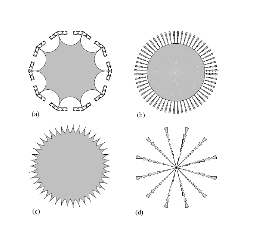
1. The mushroom is an inconvenient hollow. Therefore the resulting body (asymptotically perfect retroreflector) contains a hierarchy of mushrooms of different sizes; see fig. 14(a).

2. The difference $\varphi-\varphi^{+}$ is always nonzero; this means that the mushroom measure converges to $\eta_{\star}$ weakly, but not in norm.

3. If the semi-ellipse is substituted with a semicircle then the resulting hollow (which is also called mushroom) will also be asymptotically retroreflecting. This modified construction can be generalized to any dimension; that is, there exist multidimensional asymptotically perfect retroreflectors with mushroom-shaped hollows (for a more detailed description, see [10]).

4. Most incident particles make exactly one reflection. This means that the portion of incident particles making one reflection tends to 1 as $\varepsilon\to 0$.

3.2 Tube

The tube is a rectangle of width $a$ and height 1 with two rows of rectangles of smaller size $\delta\times\varepsilon$ taken away (see fig. 9).

Figure 9: A tube.

The lower and upper rows of rectangles are adjacent to the lower and upper sides of the tube, respectively. The distance between neighbor rectangles of each row equals 1. The opening of the tube is the left vertical side of the large rectangle. Denote by $\eta_{\varepsilon,\delta,a}$ the measure generated by the tube.

For any particle incident in the tube, with $\varphi$ and $\varphi^{+}$ being the angles of getting in and getting out, only two cases may happen: $\varphi^{+}=\varphi$ or $\varphi^{+}=-\varphi$. Letting $a\to\infty$ and $\delta\to 0$ (with $\varepsilon$ fixed), we get the semi-infinite tube where small rectangles are substituted with vertical segments of length $\varepsilon$ (see fig. 10). Studying the dynamics in this tube amounts to the following ergodic problem.

Figure 10: A semi-infinite tube.

Consider the iterated rotation of the circle by a fixed angle $\alpha$,  $\xi_{n}=\xi+\alpha n\!\!\mod\!1$,  $n=1,\,2,\ldots$ and mark the successive moments $n=n_{1}$,  $n_{1}+n_{2}$,  $n_{1}+n_{2}+n_{3},\ldots$, when $\xi_{n}\in[-\varepsilon,\,\varepsilon]\!\!\mod\!1$. Denote by $l=l_{\varepsilon}(\xi,\alpha)$ the smallest value such that $n_{1}-n_{2}+\ldots+n_{2l-1}-n_{2l}\leq 0$. Let $\mathbb{P}$ be a probability measure on $[0,\,1]\times[0,\,1]$ absolutely continuous with respect to Lebesgue measure. Then there exists the limiting distribution $p_{k}=\lim_{\varepsilon\to 0}\mathbb{P}(\{(\xi,\alpha):l_{\varepsilon}(\xi,\alpha)=k\})$, with $\sum_{k=1}^{\infty}p_{k}=1$.

In [1] this statement is proved and is then used to show that that the semi-infinite tube is an asymptotically retroreflecting "hollow" (it is not a true hollow, since it is unbounded and its boundary is not piecewise smooth). This means in this case that $\mu(\varphi^{+}=\varphi)$ goes to 1 as $\varepsilon\to 0$.

Let us show that there exists a family of true tube-shaped hollows which is asymptotically retroreflecting. To this end, define the function $H(\xi,\varphi,\varepsilon,\delta,a)$ which is equal to 0, if the billiard particle with the initial data $(\xi,\varphi)$ satisfies the equality $\varphi^{+}=\varphi$, and to 1, if $\varphi^{+}=-\varphi$ (there are no other possibilities). For the semi-infinite tube this function takes the form $H(\xi,\varphi,\varepsilon,0,+\infty)=:H(\xi,\varphi,\varepsilon)$. The asymptotical retroreflectivity of the semi-infinite tube means that

$$\lim_{\varepsilon\to 0}\int\!\!\!\int_{[0,\,1]\times[-\pi/2,\,\pi/2]}H(\xi,\varphi,\varepsilon)\,d\xi\,d\varphi=0.$$

Note that for fixed $\xi,\ \varphi$ and for $1/a$ and $\delta$ small enough the corresponding particle makes the same sequence of reflections (and therefore has the same output velocity) as in the limiting case $\delta=0,\ a=+\infty$. This implies that $H(\xi,\varphi,\varepsilon,\delta,a)$ pointwise converges (stabilizes) to $H(\xi,\varphi,\varepsilon)$ as $\delta\to 0,\ a\to+\infty$, and therefore,

$$\lim_{\delta\to 0,\,a\to+\infty}\int\!\!\!\!\int_{[0,\,1]\times[-\pi/2,\,\pi/2]}\!H(\xi,\varphi,\varepsilon,\delta,a)\,d\xi\,d\varphi=\int\!\!\!\!\int_{[0,\,1]\times[-\pi/2,\,\pi/2]}\!H(\xi,\varphi,\varepsilon)\,d\xi\,d\varphi.$$

Then, using the diagonal method, one selects $\delta=\delta(\varepsilon)$ and $a=a(\varepsilon)$ such that $\lim_{\varepsilon\to 0}a(\varepsilon)=\infty$,  $\lim_{\varepsilon\to 0}\delta(\varepsilon)=0$ and

$$\lim_{\varepsilon\to 0}\int\!\!\!\int_{[0,\,1]\times[-\pi/2,\,\pi/2]}H(\xi,\varphi,\varepsilon,\delta(\varepsilon),a(\varepsilon))\,d\xi\,d\varphi=0.$$

Thus, the corresponding family of tubes is asymptotically retroreflecting.

The obtained result can be formulated as follows.

Theorem 2.

$\eta_{\star}$ is a limit point of the set of measures generated by tubes, $\{\eta_{\varepsilon,\delta,a}\}$, equipped with the norm topology.

The tube has the following properties.

1. The tube is a convenient hollow. This property makes it possible to construct an asymptotically perfect retroreflector with identical tube-shaped hollows; see fig. 14(b).

2. The measure generated by the tube (with properly chosen $\delta=\delta(\varepsilon)$ and $a=a(\varepsilon)$) converges in norm to the retroreflector measure. In other words, the portion of retroreflected particles (that is, particles reflected in the exactly opposite direction) tends to 1.

3. We believe this construction admits a generalization to higher dimensions, but we could not prove it yet.

4. The average number of reflections in the tube is of the order of $1/\varepsilon$, and therefore, goes to infinity as $\varepsilon\to 0$.

3.3 Helmet

Another remarkable hollow called helmet was discovered and studied by P Gouveia in [5] (see also [6]). It is a curvilinear triangle, with the opening being the base of the triangle. Its lateral sides are arcs of parabolas, where the vertex of each parabola coincides with the focus of the other one (and also coincides with a vertex of the triangle at its base). The base is a segment contained in the common axis of the parabolas; see fig. 11.

Figure 11: Helmet.

The helmet is a nearly perfect retroreflector; the measure $\eta_{\rput(2.27621pt,-0.28452pt){ \scalebox{0.25}{{\psset{linewidth=2.0pt}\psecurve(-6.22403pt,-7.11317pt)(-7.11317pt,0.0pt)(-6.22403pt,7.11317pt)(-3.55658pt,14.22636pt)(0.0pt,20.11893pt)(7.11317pt,28.45274pt)}{\psset{linewidth=2.0pt}\psecurve(6.22403pt,-7.11317pt)(7.11317pt,0.0pt)(6.22403pt,7.11317pt)(3.55658pt,14.22636pt)(0.0pt,20.11893pt)(-7.11317pt,28.45274pt)}{\psset{linewidth=2.0pt}\psline(-7.11317pt,0.0pt)(7.11317pt,0.0pt)}}}\hskip 2.703pt}$ generated by this hollow satisfies ${\cal F}(\eta_{\rput(2.27621pt,-0.28452pt){ \scalebox{0.25}{{\psset{linewidth=2.0pt}\psecurve(-6.22403pt,-7.11317pt)(-7.11317pt,0.0pt)(-6.22403pt,7.11317pt)(-3.55658pt,14.22636pt)(0.0pt,20.11893pt)(7.11317pt,28.45274pt)}{\psset{linewidth=2.0pt}\psecurve(6.22403pt,-7.11317pt)(7.11317pt,0.0pt)(6.22403pt,7.11317pt)(3.55658pt,14.22636pt)(0.0pt,20.11893pt)(-7.11317pt,28.45274pt)}{\psset{linewidth=2.0pt}\psline(-7.11317pt,0.0pt)(7.11317pt,0.0pt)}}}\hskip 2.703pt})=0.9977$; this value is only $0.23\%$ smaller than the maximal value of ${\cal F}$. A body bounded by helmets is shown in figure 14(c).

The helmet has the following properties.

1. It is a convenient hollow.

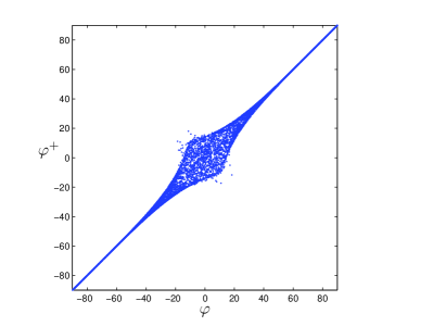
2. There always exists a small discrepancy between the initial and final directions, which is maximal for perpendicular incidence and vanishes for nearly tangent incidence. See figure 12, where the support of $\eta_{\rput(2.27621pt,-0.28452pt){ \scalebox{0.25}{{\psset{linewidth=2.0pt}\psecurve(-6.22403pt,-7.11317pt)(-7.11317pt,0.0pt)(-6.22403pt,7.11317pt)(-3.55658pt,14.22636pt)(0.0pt,20.11893pt)(7.11317pt,28.45274pt)}{\psset{linewidth=2.0pt}\psecurve(6.22403pt,-7.11317pt)(7.11317pt,0.0pt)(6.22403pt,7.11317pt)(3.55658pt,14.22636pt)(0.0pt,20.11893pt)(-7.11317pt,28.45274pt)}{\psset{linewidth=2.0pt}\psline(-7.11317pt,0.0pt)(7.11317pt,0.0pt)}}}\hskip 2.703pt}$ is shown. The figure is obtained numerically, by calculating the pairs $(\varphi,\varphi^{+})$ for $10\,000$ values of $\varphi$ chosen at random. This means that, when illuminated, the contour of the retroreflector is seen best of all, which is useful for visual reconstruction of its shape.

Figure 12: The support of the measure generated by helmet is shown. It is obtained numerically by calculating 10 000 randomly chosen pairs $(\varphi,\varphi^{+})$.

3. We do not know if there exist multidimensional generalizations of this shape. By now, the greatest value of the parameter ${\cal F}$ attained by numerical simulation in three dimensions equals $0.9$.

4. For most particles, the number of successive reflections equals 3, although 4, 5, etc. (up to infinity) reflections are also possible. When the number of reflection increases, the number of corresponding particles rapidly decreases.

5. The boundary of helmet is the graph of a function. This means that this shape may be easy for manufacturing.

3.4 Notched angle

This shape is depicted in figure 13, and the corresponding body, in figure 14(d). Here we point out its properties.

Figure 13: Notched angle.

1. Notched angle is a convenient hollow.

2. The corresponding measure converges in norm to the retroreflector measure $\eta_{\star}$.

3. We are unaware of multidimensional generalizations of this shape.

4. The mean number of reflections in notched angle goes to infinity as $\alpha$ tends to zero.

5. The boundary of the notched angle is the graph of a function.

The rigorous definition of this shape and the proof of its retroreflectivity are given in the next section 4.

3.5 Comparison table for retroreflectors

Here we put together the billiard retroreflectors. For convenience, their properties are tabulated below. The limiting values of $r$ are equal to 1 in all shapes, except for the helmet.

In figure 14, four bodies with boundaries formed by corresponding retroreflecting hollows are shown.

Figure 14: Bodies with boundaries formed by retroreflecting hollows: (a) mushroom; (b) tube; (c) helmet; (d) notched angle.

As concerns possible applications of these shapes, each of them seems to have some advantages and disadvantages. Tube and notched angle ensure exact direction reversal, while in mushroom and helmet a small discrepancy between initial and final directions is always present, which can make them inefficient at very large distances. On the other hand, the number of reflections for the most part of particles in mushroom and helmet equals 1 and 3, respectively, while the mean number of reflections goes to infinity for sequences of bodies representing tube and notched angle, which may imply need for high quality of reflecting boundary.

4 Notched angle

Consider two isosceles triangles, $\bar{A}\bar{O}\bar{B}$ and $\bar{A}^{\prime}\bar{O}\bar{B}^{\prime}$, with the common vertex $\bar{O}$ and require that the base of one of them is contained in the base of the other one, $\bar{A}\bar{B}\subset\bar{A}^{\prime}\bar{B}^{\prime}$. The segment $\bar{A}\bar{B}$ is horizontal in figure 13. Denote $\measuredangle\bar{A}\bar{O}\bar{B}=\alpha$ and $\measuredangle\bar{A}^{\prime}\bar{O}\bar{B}^{\prime}=\alpha+\beta$. Draw two broken lines with horizontal and vertical segments with the origin at $\bar{A}$ and $\bar{B}$, respectively, and require that the vertices of the first line belong to the segments $\bar{O}\bar{A}$ and $\bar{O}\bar{A}^{\prime}$, and the vertices of the second line, to the segments $\bar{O}\bar{B}$ and $\bar{O}\bar{B}^{\prime}$; see figure 13. The endpoint of both broken lines is $\bar{O}$; both lines have infinitely many segments and finite length. We will consider the "hollow" $(\Omega,I)$ with the opening $I=I_{\alpha}=\bar{A}\bar{B}$ and with the set $\Omega=\Omega_{\alpha,\beta}$ bounded by $\bar{A}\bar{B}$ and the two broken lines. This "hollow" will be called a notched angle with the size $(\alpha,\beta)$, or just an $(\alpha,\beta)$-angle. The boundary $\partial\Omega$ is not piecewise smooth ($\bar{O}$ is a limit point for singular points of $\partial\Omega$), therefore the word hollow is put in quotes; however, the measure generated by this "hollow" is defined in the standard way. This measure depends only on $\alpha$ and $\beta$ and is denoted by $\eta_{\alpha,\beta}$.

Theorem 3.

There exists a function $\beta=\beta(\alpha)$,  $\lim_{\alpha\to 0}(\beta/\alpha)=0$ such that $\eta_{\alpha,\beta}$ converges in norm to the retroreflector measure $\eta_{\star}$ as $\alpha\to 0$.

Remark 9.

Using this theorem, one easily constructs a family of true hollows for which convergence in norm to $\eta_{\star}$ takes place. Namely, draw a straight line $CD$ parallel to $\bar{A}\bar{B}$ at a small distance $\delta$ from $\bar{O}$; the true hollow is the part of the original "hollow" situated between $\bar{A}\bar{B}$ and $CD$, with the same opening (see fig. 13). The measure generated by this hollow tends to $\eta_{\star}$ as $\alpha\to 0$, with properly chosen $\beta=\beta(\alpha)$ and $\delta=\delta(\alpha)$ vanishing when $\alpha\to 0$.

Proof.

For any initial data $\xi$,  $\varphi$ the angle of getting away $\varphi^{+}=\varphi^{+}_{\alpha,\beta}(\xi,\varphi)$ satisfies either $\varphi^{+}=\varphi$, or $\varphi^{+}=-\varphi$. To prove the theorem, it suffices to check that the measure $\mu$ of the set of initial data $\xi$,  $\varphi$ satisfying $\varphi^{+}_{\alpha,\beta}(\xi,\varphi)=-\varphi$ and $|\varphi|>\alpha$ tends to 0 as $\alpha\to 0$,  $\beta=\beta(\alpha)$.

Make a uniform extension along the horizontal axis in such a way that the resulting angle $\bar{A}\bar{O}\bar{B}$ becomes right. Then the angle $\bar{A}^{\prime}\bar{O}\bar{B}^{\prime}$ becomes equal to $\pi/2+\gamma$,  $\gamma=\gamma(\alpha,\beta)$ (see fig. 15), besides the conditions $\alpha\to 0$,  $\beta/\alpha\to 0$ imply that $\gamma\to 0$. This extension takes the $(\alpha,\beta)$-angle to a $(\pi/2,\delta)$-angle, takes each billiard trajectory to another billiard trajectory, and takes the measure $\frac{1}{2}\cos\varphi\,d\varphi\,d\xi$ to a measure absolutely continuous with respect to it.

The vertices of the resulting notched angle will be denoted by $O$,  $A$,  $B$,  $A^{\prime}$,  $B^{\prime}$, without overline, in order to distinguish them from the previous notation.

Without loss of generality we assume that $|OA|=|OB|=1$. Introduce the uniform parameter $\xi$ on the segment $AB$, where $A$ corresponds to the value $\xi=0$ and $B$, to the value $\xi=1$. Extend the trajectory of an incident particle with initial data $\xi$,  $\varphi<-\pi/4$ until the intersection with the extension of $OA$. Denote by $\tilde{x}_{0}$ the distance from $O$ to the point of intersection; see fig. 15. (In what follows, a point on the ray $OA$ or $OB$ will be identified with the distance from the vertex $O$ to this point.) In the new representation, the particle starts the motion at a point $\tilde{x}_{0}$ and intersects the segment $AB$ at a point $\xi$ and at an angle $\varphi$. Continuing the straight-line motion, it intersects the side $OB$ at a point $x_{1}$  $(0<x_{1}<1)$, then makes one or two reflections from the broken line and intersects $OB$ again at a point $\tilde{x}_{1}$. Denote $x_{1}/\tilde{x}_{0}=\lambda$; obviously one has $0<\lambda<1$. The value $\lambda$ is the tangent of the angle of trajectory inclination relative to $OA$; thus, one has $\varphi=-\pi/4-\arctan\lambda$. It is convenient to change the variables in the space of particles getting into the hollow at an angle $\varphi<-\pi/4$. Namely, we pass from the parameters $\xi\in[0,\,1]$,  $\varphi\in[-\pi/2,\,-\pi/4]$ to the parameters $\lambda\in[0,\,1]$,  $\tilde{x}_{0}\in[1,\,1/\lambda]$. This change of variables can be written as $\xi=\frac{\lambda}{1-\lambda}\,(\tilde{x}_{0}-1)$,  $\varphi=\pi/4+\arctan\lambda$; it transforms the measure $\frac{1}{2}\,\cos\varphi\,d\varphi\,d\xi$ into the measure $\frac{\lambda}{2\sqrt{2}(1+\lambda^{2})^{3/2}}\,d\lambda\,d\tilde{x}_{0}$.

Figure 15: The reduced notched angle.

By considering successive alternating reflections of the particle from the broken lines resting on the sides $OB$ and $OA$, we define the sequence of values $x_{1}$,  $\tilde{x}_{1}$, …, $x_{m-1}$,  $\tilde{x}_{m-1}$. Obviously, all these values are smaller than 1. Then the particle gets out of the hollow and intersects the extension of the side $OA$ or $OB$ at a point $x_{m}>1$. If $m$ is even, then the intersection with $OA$ takes place, and $\varphi^{+}=\varphi$. If $m$ is odd, then intersection with $OB$ takes place, with $\varphi^{+}=-\varphi$. Clearly, $m$ depends on the initial data $\tilde{x}_{0}$,  $\lambda$ and on the parameter $\gamma$,  $m=m_{\gamma}(\tilde{x}_{0},\lambda)$.

Statement 2.

For any $\lambda$, the measure of the set of values $\tilde{x}_{0}$ such that $m_{\gamma}(\tilde{x}_{0},\lambda)$ is odd, goes to $0$ as $\gamma\to 0$.

Let us derive the theorem from this statement. Indeed, let $f_{\gamma}(\lambda)$ be the measure of the set indicated in the statement, $f_{\gamma}(\lambda)=|\{\tilde{x}_{0}:m_{\gamma}(\tilde{x}_{0},\lambda)\text{ is odd}\,\}|$. Introduce the measure $\eta$ on the segment $[0,\,1]$ according to $d\eta(\lambda)=\frac{\lambda\,d\lambda}{2\sqrt{2}(1+\lambda^{2})^{3/2}}$; then $\int_{0}^{1}f_{\gamma}(\lambda)\,d\eta(\lambda)$ is the measure of the set of initial values $(\lambda,\tilde{x}_{0})$ such that $m_{\gamma}(\tilde{x}_{0},\lambda)$ is odd. The value $f_{\gamma}(\lambda)$ does not exceed the full Lebesgue measure of the segment $[1,\,\lambda^{-1}]$,

$$f_{\gamma}(\lambda)\leq\lambda^{-1}-1,$$ (11)

and the function $\lambda^{-1}-1$ is integrable relative to $\eta$, $\int_{0}^{1}(\lambda^{-1}-1)\,d\eta(\lambda)=\frac{\sqrt{2}-1}{2\sqrt{2}}$. According to statement 2, for any $\lambda$ holds

$$\lim_{\gamma\to 0}f_{\gamma}(\lambda)=0.$$ (12)

Taking into account (11) and (12) and applying Lebesgue’s dominated convergence theorem, one gets

$$\lim_{\gamma\to 0}\int_{0}^{1}f_{\gamma}(\lambda)\,d\eta(\lambda)=0.$$

This means that the measure of the set of values $(\xi,\varphi)$,  $\varphi\leq-\pi/4$ for which the equality $\varphi^{+}_{\pi/2,\gamma}(\xi,\varphi)=-\varphi$ is valid, tends to 0 as $\gamma\to 0$. The same statement, due to the axial symmetry of the billiard, is also valid for $\varphi\geq\pi/4$.

Now make a uniform contraction along the abscissa axis transforming the $(\pi/2,\gamma)$-angle into an $(\alpha,\beta)$-angle (where $\beta$ depends on $\gamma$ and $\alpha$). Taking into account that the measures generated by these angles are mutually absolutely continuous, we get that the measure $\mu(\{(\xi,\varphi):|\varphi|\geq\alpha\text{ and }\varphi^{+}_{\alpha,\beta}(\xi,\varphi)=-\varphi\})$ goes to 0 at fixed $\alpha$ and $\beta\to 0$.

Finally, choose a diagonal family of parameters $\alpha$,  $\beta(\alpha)$,  $\lim_{\alpha\to 0}(\beta(\alpha)/\alpha)=0$ such that the measure

$$\mu(\{(\xi,\varphi):|\varphi|\geq\alpha\,\text{ and }\,\varphi^{+}_{\alpha,\beta(\alpha)}(\xi,\varphi)=-\varphi\})\to 0\quad\text{as}\ \ \alpha\to 0.$$

It remains to notice that $\mu(\varphi^{+}_{\alpha,\beta(\alpha)}=-\varphi)\leq\mu(|\varphi|\geq\alpha\text{ and }\varphi^{+}_{\alpha,\beta(\alpha)}=-\varphi)+\mu(|\varphi|<\alpha)$ and $\mu(|\varphi|<\alpha)\to 0$ as $\alpha\to 0$. This finishes the proof of theorem 3. ∎

Proof of statement 2. Note that the broken lines intersect with the sides $OA$ and $OB$ at the points $x=e^{-n\delta}$,  $n=0,\,1,\,2,\ldots$, where $\delta$ is defined by the relation $\tanh\delta=\sin\gamma$. Consider an arbitrary pair of values $x_{k}$,  $\tilde{x}_{k}$; they belong to a segment bounded by a pair of points $x=e^{-n\delta}$ and $e^{-(n+1)\delta}$. Consider also the right triangle, with the hypotenuse being this segment and with the legs being segments of the broken line.

Two cases may happen: either (I) $x_{k}/\tilde{x}_{k-1}=\lambda$ or (II) $x_{k}/\tilde{x}_{k-1}=\lambda^{-1}$, the first case corresponding to the "forward" motion in the direction of the point $O$, and the second, to the "backward" motion. Introduce the local variable $\zeta$ on the hypotenuse according to $x=e^{-n\delta}[1+\zeta(e^{-\delta}-1)]$ (see fig. 16). Thus, the value $\zeta=0$ corresponds to the point $x=e^{-n\delta}$, and $\zeta=1$, to the point $x=e^{-(n+1)\delta}$. The sequences $x_{k}$,  $\tilde{x}_{k}$ generate two sequences $\zeta_{k}$,  $\tilde{\zeta}_{k}\in(0,\,1)$ and an integer-valued sequence $n_{k}$. Consider the two cases separately.

(I) $x_{k}/\tilde{x}_{k-1}=\lambda$.

(a) If $0<\zeta_{k}<\lambda$, then $\tilde{\zeta}_{k}=\lambda^{-1}\zeta_{k}$ and the particle, after leaving the triangle, continues the forward motion, that is, $x_{k+1}/\tilde{x}_{k}=\lambda$.

(b) If $\lambda<\zeta_{k}<1$, then $\tilde{\zeta}_{k}=1+\lambda-\zeta_{k}$ and the particle, after leaving the triangle, proceeds to the backward motion, $x_{k+1}/\tilde{x}_{k}=\lambda^{-1}$.

(II) $x_{k}/\tilde{x}_{k-1}=\lambda^{-1}$. In this case one has $\tilde{\zeta}_{k}=\lambda\zeta_{k}$ and the backward motion continues, $x_{k+1}/\tilde{x}_{k}=\lambda^{-1}$.

Figure 16: Dynamics in a small right triangle.

Introduce the logarithmic scale $z=-\frac{1}{\delta}\,\ln x$; then one gets a sequence of values $\tilde{z}_{0}$,  $z_{1}$,  $\tilde{z}_{1},\ldots,z_{m-1}$,  $\tilde{z}_{m-1}$,  $z_{m}$. The first and the last term in this sequence are negative, and the rest of the terms are positive. One has $-\frac{1}{\delta}\ln\frac{1}{\lambda}<\tilde{z}_{0}<0$. The following equations establish the connection between $z_{k},\ \tilde{z}_{k}$ and $\zeta_{k},\ \tilde{\zeta}_{k}$.

$$z_{k}=n_{k}-\frac{1}{\delta}\ln[1+\zeta_{k}(e^{-\delta}-1)],$$ (13)

$$\tilde{z}_{k}=n_{k}-\frac{1}{\delta}\ln[1+\tilde{\zeta}_{k}(e^{-\delta}-1)].$$ (14)

As $\delta\to 0$, one gets $z_{k}=n_{k}+\zeta_{k}+O(\delta)$,  $\tilde{z}_{k}=n_{k}+\tilde{\zeta}_{k}+O(\delta)$, where the estimates $O(\delta)$ are uniform over all $k$ and all initial data; thus, $\zeta_{k}$ and $\tilde{\zeta}_{k}$ are approximately equal to the fractional parts of $z_{k}$ and $\tilde{z}_{k}$, respectively.

For several initial values $k=1,\,2,\ldots,k_{\delta}-1$ corresponding to the forward motion of the particle, according to (Ia) one has

$$z_{k}=\tilde{z}_{k-1}+\frac{1}{\delta}\ln\frac{1}{\lambda};\quad\quad\quad 0<\zeta_{k}<\lambda,\quad\tilde{\zeta}_{k}=\lambda^{-1}\zeta_{k};\quad\quad\quad z_{k+1}=\tilde{z}_{k}+\frac{1}{\delta}\ln\frac{1}{\lambda}.$$ (15)

Here and in the following formulas (16),(17), $\,\zeta_{k}$ is determined by $z_{k}$ and $\tilde{z}_{k}$ is determined by $\tilde{\zeta}_{k}$, according to (13) and (14). For the value $k=k_{\delta}$ corresponding to the transition from the forward motion to the backward one, according to (Ib) one has

$$z_{k_{\delta}}=\tilde{z}_{k_{\delta}-1}+\frac{1}{\delta}\ln\frac{1}{\lambda};\ \quad\lambda<\zeta_{k_{\delta}}<1,\quad\tilde{\zeta}_{k_{\delta}}=1+\lambda-\zeta_{k_{\delta}};\quad\ z_{k_{\delta}+1}=\tilde{z}_{k_{\delta}}-\frac{1}{\delta}\ln\frac{1}{\lambda}.$$ (16)

Finally, for the values $k=k_{\delta}+1,\ldots,m-1$ corresponding to the backward motion, according to (II) one has

$$z_{k}=\tilde{z}_{k-1}-\frac{1}{\delta}\ln\frac{1}{\lambda};\quad\quad\quad\tilde{\zeta}_{k}=\lambda\zeta_{k};\quad\quad\quad z_{k+1}=\tilde{z}_{k}-\frac{1}{\delta}\ln\frac{1}{\lambda}.$$ (17)

Notice that in figure 15 one has $k_{\delta}=2$.

The formulas (13)–(17) define iterations of the pairs of mappings

$$\tilde{z}_{k-1}\mapsto z_{k}\mapsto\tilde{z}_{k}$$ (18)

with positive integer time $k$. These mappings commute with the shift $z\mapsto z+1$. The initial value $\tilde{z}_{0}$ satisfies $\tilde{z}_{0}\in(-\frac{1}{\delta}\ln\frac{1}{\lambda},\,0)$, and the relation $z_{m}\in(-\frac{1}{\delta}\ln\frac{1}{\lambda},\,0)$ defines the time $m$ when the corresponding value leaves the positive semi-axis $z\geq 0$ and the process stops.

During the forward motion, the first mapping in (18) increases the value of $z$ by $\frac{1}{\delta}\ln\frac{1}{\lambda}$, and the second one changes it by a value smaller than 1. During the backward motion, the first mapping decreases $z$ by $\frac{1}{\delta}\ln\frac{1}{\lambda}$, and the second mapping changes it again by a value smaller than 1. Therefore, if the initial value satisfies $\tilde{z}_{0}\in(-\frac{1}{\delta}\ln\frac{1}{\lambda}+2k,\,-2k)$ with $k>k_{\delta}$, then $z_{2k_{\delta}}\in(-\frac{1}{\delta}\ln\frac{1}{\lambda},\,0)$, and so, $m=2k_{\delta}$. This means that $m$ is always even, except for a small portion $4k/(\frac{1}{\delta}\ln\frac{1}{\lambda})$ of the initial values. Thus, to complete the proof of statement 2, we only need a result stating that the transition time $k_{\delta}$ remains bounded when $\delta\to 0$.

Due to invariance with respect to integer shifts, the formulas (13)–(17) determine iterated maps on the unit circumference with the coordinate $z\!\!\mod\!1$. The value $k_{\delta}=k_{\delta}(\tilde{z}_{0}\!\!\mod\!1)$ is a Borel measurable function; it can be interpreted as a random variable, where the random event is represented by the variable $\tilde{z}_{0}\!\!\mod\!1$ on the circumference with Lebesgue measure.

Statement 3.

The limiting distribution of $k_{\delta}$ as $\delta\to 0$ equals $P_{\lambda}(k)=\lambda^{k-1}(1-\lambda)$,  $k=1,\,2,\ldots$.

Let us derive statement 2 using statement 3. Indeed, one has $1-P_{\lambda}(1)-\ldots-P_{\lambda}(k)=\lambda^{k}$. Take an arbitrary $\varepsilon>0$ and choose $k$ such that $\lambda^{k}<\varepsilon$. Then, using statement 3, choose $\delta_{0}>0$ such that $\mathbb{P}(k_{\delta}>k)<\varepsilon$ for any $\delta<\delta_{0}$. This implies that the inequality $|\tilde{z}_{0}-z_{2k_{\delta}}|<2k$ holds with the probability at least $1-\varepsilon$. Therefore, if $\delta$ satisfies $\delta<\delta_{0}$ and $4k/(\frac{1}{\delta}\ln\frac{1}{\lambda})<\varepsilon$, the relative Lebesgue measure of the set of points $\tilde{z}_{0}\in(-\frac{1}{\delta}\ln\frac{1}{\lambda},\,0)$ producing the value $m=2k_{\delta}$ is greater than $1-2\varepsilon$. Passing from the variable $\tilde{z}_{0}$ to the variable $\tilde{x}_{0}=e^{-\delta\tilde{z}_{0}}$, one concludes that Lebesgue measure of the set of values of $\tilde{x}_{0}$ corresponding to odd $m$ tends to 0 as $\delta\to 0$. This completes the proof of statement 2.  $\Box$

Proof of statement 3. For convenience write down iterations of the pair of mappings until the transition time $k_{\delta}$ in the form

$$z_{k}=\tilde{z}_{k-1}+\frac{1}{\delta}\ln\frac{1}{\lambda}\!\!\mod\!1,\quad\tilde{z}_{k}=f_{\delta}^{-1}(z_{k})\quad(1\leq k<k_{\delta}),$$ (19)

where the function $f_{\delta}$ is given by relations (13), (14) and (15); one easily derives that $f_{\delta}(\tilde{z})=\zeta^{-1}(\lambda\,\zeta(\tilde{z}))$, with $\zeta(z)=(1-e^{-\delta z})/(1-e^{-\delta})$. The function $f_{\delta}$ is monotone and injectively maps the circumference ${\mathbb{R}}/{\mathbb{Z}}$ with the coordinate $z\!\!\mod\!1$ into itself, and is discontinuous at $0\!\!\mod\!1$. In the limit $\delta\to 0$,  $f_{\delta}(\tilde{z})$ uniformly converges to $\lambda\tilde{z}$ and the derivative $f^{\prime}_{\delta}$ uniformly converges to $\lambda$; the last means that

$$\lim_{\delta\to 0}\inf f^{\prime}_{\delta}=\lim_{\delta\to 0}\sup f^{\prime}_{\delta}=\lambda.$$ (20)

The iterations (19) are defined while $z_{k}\in\text{Range}(f_{\delta})$; the first moment when $z_{k}\not\in\text{Range}(f_{\delta})$ is $k=k_{\delta}$.

Denote by $\mathcal{A}_{\delta}(k)=\{\tilde{z}_{0}\!\!\mod\!1:\,k_{\delta}(\tilde{z}_{0}\!\!\mod\!1)>k\}$ the set of initial values $\tilde{z}_{0}\!\!\mod\!1\in{\mathbb{R}}/{\mathbb{Z}}$ for which the inequality $k_{\delta}>k$ holds true. Then one has $\mathbb{P}(k_{\delta}>k)=|\mathcal{A}_{\delta}(k)|$, where $|\cdot|$ means Lebesgue measure on ${\mathbb{R}}/{\mathbb{Z}}$. The following inductive formulas are valid: $\mathcal{A}_{\delta}(0)={\mathbb{R}}/{\mathbb{Z}}$ and $\mathcal{A}_{\delta}(k+1)=f_{\delta}(\mathcal{A}_{\delta}(k))-\frac{1}{\delta}\ln\frac{1}{\lambda}\!\!\mod\!1$. They imply that $|\mathcal{A}_{\delta}(0)|=1$ and

$$\inf_{z}f^{\prime}_{\delta}(z)\leq\frac{|\mathcal{A}_{\delta}(k+1)|}{|\mathcal{A}_{\delta}(k)|}\leq\sup_{z}f^{\prime}_{\delta}(z).$$ (21)

Formulas (20) and (21) imply that $\lim_{\delta\to 0}|\mathcal{A}_{\delta}(k)|=\lambda^{k}$; therefore $\lim_{\delta\to 0}\mathbb{P}(k_{\delta}=k)=\lim_{\delta\to 0}(\mathcal{A}_{\delta}(k-1))-\mathcal{A}_{\delta}(k)))=\lambda^{k-1}(1-\lambda)$. Statement 3 is proved.      $\Box$

5 Appendix

5.1 Convergence of measures generated by rectangular hollows

Both the measures $\eta^{\varepsilon}_{\sqcup}$ and the limiting measure $\frac{1}{2}(\eta_{0}+\eta_{\star})$ have a cross-shaped support, as shown in figure 17.

Figure 17: The support of the semi-retroreflecting measure.

Therefore, the density of $\eta^{\varepsilon}_{\sqcup}$ can be written down as

$$\rho_{\varepsilon}(\varphi)\,\delta(\varphi-\varphi^{+})+\Big{(}\frac{1}{2}\cos\varphi-\rho_{\varepsilon}(\varphi)\Big{)}\,\delta(\varphi+\varphi^{+}),$$

and the density of $\frac{1}{2}(\eta_{0}+\eta_{\star})$ equals

$$\frac{1}{4}\cos\varphi\,(\delta(\varphi-\varphi^{+})+\delta(\varphi+\varphi^{+})).$$

Define the function $f_{\varepsilon}(\xi,\varphi)=\left\{\begin{array}[]{rl}1,&\text{if }\ \varphi^{+}(\xi,\varphi)=\varphi\\ -1,&\text{if }\ \varphi^{+}(\xi,\varphi)=-\varphi\end{array}\right.$; then one has

$$\rho_{\varepsilon}(\varphi)-\Big{(}\frac{1}{2}\cos\varphi-\rho_{\varepsilon}(\varphi)\Big{)}=\cos\varphi\cdot\int_{0}^{1}f_{\varepsilon}(\xi,\varphi)\,d\xi.$$

The value of $f_{\varepsilon}$ is determined from the parity of the number of reflections in the tube and can be easily found by unfolding of the billiard trajectory (see fig. 18).

Figure 18: The unfolded billiard trajectory in the tube.

One easily sees that $f(\xi,\varphi)=1$, if $\lfloor\xi+\frac{2}{\varepsilon}\tan\varphi\rfloor$ is odd and $f(\xi,\varphi)=-1$, if $\lfloor\xi+\frac{2}{\varepsilon}\tan\varphi\rfloor$ is even, where $\lfloor\ldots\rfloor$ means the integer part of a real number.

To prove the weak convergence, it suffices to check that for any $-\pi/2<\Phi_{1}<\Phi_{2}<\pi/2$,

$$\lim_{\varepsilon\to 0}\int_{0}^{1}\!\!\!\int_{\Phi_{1}}^{\Phi_{2}}f_{\varepsilon}(\xi,\varphi)\,\cos\varphi\,d\varphi\,d\xi=0.$$ (22)

Fix $\xi$ and denote $\varphi_{m}=\arctan(\frac{\varepsilon}{2}(m-\xi))$. One has $f_{\varepsilon}(\xi,\varphi)=1$, if $\varphi_{2n-1}<\varphi<\varphi_{2n}$ and $f_{\varepsilon}(\xi,\varphi)=-1$, if $\varphi_{2n}<\varphi<\varphi_{2n+1}$. One easily deduces from this that the integral $\int_{\Phi_{1}}^{\Phi_{2}}f_{\varepsilon}(\xi,\varphi)\,\cos\varphi\,d\varphi$ converges to zero as $\varepsilon\to 0$ (and is obviously bounded, $|\int_{\Phi_{1}}^{\Phi_{2}}f_{\varepsilon}(\xi,\varphi)\,\cos\varphi\,d\varphi|<2$), and therefore, the convergence in (22) takes place.

5.2 Convergence of measures generated by triangular hollows

The images of the triangular hollow $AOB$ obtained by the unfolding procedure form a polygon inscribed in a circle (see figure 19). Introduce the angular coordinate $x\!\!\mod\!2\pi$ (measured clockwise from the point $B$) on the circumference. Given an incident particle, denote by $x$ and $x^{+}$ the two points of intersection of the unfolded trajectory with the circumference. We are given $\measuredangle AOB=\varepsilon$; therefore $x\in[0,\,\varepsilon]$.

Figure 19: The unfolded billiard trajectory in the triangle.

Denote by $\phi$ the angle between the direction vector of the unfolded trajectory and the radius at the first point of intersection; then the angle at the second point of intersection will be $-\phi$. Both angles are measured counterclockwise from the corresponding radius to the velocity; so, for example, $\phi>0$ in figure 19.

One has $x^{+}=x+\pi-2\phi$. The number of intersections of the unfolded trajectory with the images of the radii $OA$ and $OB$ coincides with the number of reflections of the true billiard trajectory and is equal to $n=n_{\varepsilon}(x,\phi)=\lfloor\frac{x+\pi-2\phi}{\varepsilon}\rfloor$. In figure 19, $n=3$.

Denote by $\varphi$ and $\varphi^{+}$, respectively, the angles formed by the velocity of the true billiard trajectory with the outer normal to $AB$ at the moments of the first and second intersection with the opening $AB$. One easily sees that

$$|\varphi-\phi|\leq\varepsilon/2\quad\text{and}\quad|\varphi^{+}-(-1)^{n+1}\phi|\leq\varepsilon/2.$$ (23)

The mapping $(x,\phi)\mapsto(\varphi,\varphi^{+})$ defines a measure preserving one-to-one correspondence between a subspace of the space $[0,\,\varepsilon]\times[-\pi/2,\,\pi/2]$ with the measure $\frac{1}{2\sin(\varepsilon/2)}dx\cdot\frac{1}{2}\cos\phi\,d\phi$ and the space $\Box=[-\pi/2,\,\pi/2]^{2}$ with the measure $\eta^{\varepsilon}_{\vee}$. Consider also the mapping

$$(x,\phi)\mapsto(\phi,(-1)^{n_{\varepsilon}(x,\phi)+1}\phi)$$

and the measure $\tilde{\eta}^{\varepsilon}_{\vee}$ induced on $\Box$ by this mapping. One easily deduces from the inequalities (23) that the difference $\eta^{\varepsilon}_{\vee}-\tilde{\eta}^{\varepsilon}_{\vee}$ weakly converges to zero as $\varepsilon\to 0$; therefore it is sufficient to prove the weak convergence

$$\tilde{\eta}^{\varepsilon}_{\vee}\to\frac{1}{2}(\eta_{0}+\eta_{\star})\quad\text{as}\ \ \varepsilon\to 0.$$ (24)

Introduce the function

$$g_{\varepsilon}(x,\phi)=\left\{\begin{array}[]{rl}1,&\text{if }\ n_{\varepsilon}(x,\phi)\ \text{ is odd}\\ -1,&\text{if }\ n_{\varepsilon}(x,\phi)\ \text{ is even}\end{array}\right..$$

Similarly to the previous subsection 5.1, it suffices to prove that for any $-\pi/2<\Phi_{1}<\Phi_{2}<\pi/2$,

$$\lim_{\varepsilon\to 0}\frac{1}{\varepsilon}\int_{0}^{\varepsilon}\!\!\!\int_{\Phi_{1}}^{\Phi_{2}}g_{\varepsilon}(x,\phi)\,\cos\phi\,d\phi\,dx=0.$$ (25)

Fix $x\in[0,\,\varepsilon]$ and put $\phi_{m}=\frac{1}{2}(x+\pi-m\varepsilon)$. One has $g_{\varepsilon}(x,\phi)=1$, if $\phi_{2n-1}<\phi<\phi_{2n}$ and $g_{\varepsilon}(x,\phi)=-1$, if $\phi_{2n}<\phi<\phi_{2n+1}$. We easily get that the integral $\int_{\Phi_{1}}^{\Phi_{2}}g_{\varepsilon}(x,\phi)\,\cos\phi\,d\phi$ uniformly converges to zero as $\varepsilon\to 0$ (actually, it is less than $2\varepsilon$), and therefore, the convergence in (25) also takes place.

References

- [1] P. Bachurin, K. Khanin, J. Marklof and A. Plakhov. Perfect retroreflectors and billiard dynamics. Submitted.
- [2] K. I. Borg, L. H. Söderholm and H. Essén. Force on a spinning sphere moving in a rarefied gas. Physics of Fluids 15, 736-741 (2003).
- [3] L. Bunimovich. Mushrooms and other billiards with divided phase space. Chaos 11, 802-808 (2001).
- [4] J. E. Eaton. On spherically symmetric lenses. Trans. IRE Antennas Propag. 4, 66-71 (1952).
- [5] P. D. F. Gouveia. Computação de Simetrias Variacionais e Optimização da Resistência Aerodinâmica Newtoniana. Ph.D. Thesis, Universidade de Aveiro, Portugal (2007).
- [6] P. Gouveia, A. Plakhov and D. Torres. Two-dimensional body of maximum mean resistance. Applied Math. and Computation 215, 37–52 (2009). doi:10.1016/j.amc.2009.04.030
- [7] S. G. Ivanov and A. M. Yanshin. Forces and moments acting on bodies rotating around a symmetry axis in a free molecular flow. Fluid Dyn. 15, 449 (1980).
- [8] K. Moe and M. M. Moe. Gas-surface interactions and satellite drag coefficients. Planet. Space Sci. 53, 793-801 (2005).
- [9] I. Newton. Philosophiae naturalis principia mathematica. 1686.
- [10] A Plakhov. Billiards in unbounded domains reversing the direction of motion of a particle. Russ. Math. Surv. 61, 179-180 (2006).
- [11] A Plakhov. Billiards and two-dimensional problems of optimal resistance. Arch. Ration. Mech. Anal. 194, 349-382 (2009). DOI 10.1007/s00205-008-0137-1.
- [12] A. Plakhov and P. Gouveia. Problems of maximal mean resistance on the plane. Nonlinearity 20, 2271-2287 (2007).
- [13] A. Plakhov. Scattering in billiards and problems of Newtonian aerodynamics. Russ. Math. Surv. 64, 873–938 (2009).
- [14] S. Tabachnikov. Billiards. Paris: Société Mathématique de France (1995).
- [15] C.-T. Wang. Free molecular flow over a rotating sphere. AIAA J. 10, 713 (1972).