Star Formation Timescales and the Schmidt Law

Abstract

We offer a simple parameterization of the rate of star formation in galaxies. In this new approach, we make explicit and decouple the timescales associated (a) with disruptive effects the star formation event itself, from (b) the timescales associated with the cloud assembly and collapse mechanisms leading up to star formation. The star formation law in near-by galaxies, as measured on sub-kiloparsec scales, has recently been shown by Bigiel et al. to be distinctly non-linear in its dependence on total gas density. Our parameterization of the spatially resolved Schmidt-Sanduleak relation naturally accommodates that dependence. The parameterized form of the relation is $\rho_{*}\sim\epsilon\rho_{g}/(\tau_{s}+\rho_{g}^{-n})$, where $\rho_{g}$ is the gas density, $\epsilon$ is the efficiency of converting gas into stars, and $\rho_{g}^{-n}$ captures the physics of cloud collapse. Accordingly at high gas densities quiescent star formation is predicted to progress as $\rho_{*}\sim\rho_{g}$, while at low gas densities $\rho_{*}\sim\rho_{g}^{1+n}$, as is now generally observed. A variable efficiency in locally converting gas into stars as well as the unknown plane thickness variations from galaxy to galaxy, and radially within a given galaxy, can readily account for the empirical scatter in the observed (surface density rather than volume density) relations, and also plausibly account for the noted upturn in the relation at very high apparent projected column densities.

1 Introduction

The Schmidt Law has become widely synonymous with any power-law relation between a (local or even global) star formation rate indicator (be it individual OB stars, HII regions, H$\alpha$ luminosity, UV luminosity, re-radiated 24$\mu$m radiation or the strength of a [C IV] cooling line) and a corresponding measure of gas density (originally HI and now more frequently H₂, or a summed combination of the two). Schmidt (1957, 1963) first proposed such a formalism after noting that within the context of the Milky Way the gas scale height (the fuel for star formation) was larger than the O-star scale height (the result of star formation) suggesting a non-linear (plausibly a power-law) causally connected relationship between the two. Schmidt concluded that the exponent connecting gas density to star formation had a value of n $\sim$ 2. Subsequently, (with the exception of a solitary paper by Guibery, Lequeux & Viallefond 1978, again dealing with the Milky Way star formation and gas scale heights) little interest in this topic was visible for more than a decade.

The field became active again when some years later Sanduleak (1968) offered a novel calibration of the Schmidt Law in an extragalactic context. Rather than working with scale heights he examined the relationship between neutral hydrogen gas surface densities and the projected surface densities of recently-formed and individually resolved OB stars. We refer hereafter to this spatially resolved correlation of star formation tracers with projected gas surface density as the Schmidt-Sanduleak Law, so as to clearly distinguish it from the global relation linking the total star formation rate with total gas content, often referred to as the Schmidt-Kennicutt Law. For OB stars and neutral hydrogen gas in the SMC Sanduleak found $\Sigma_{stars}\sim\Sigma^{1.84\pm 0.14}_{gas}$.

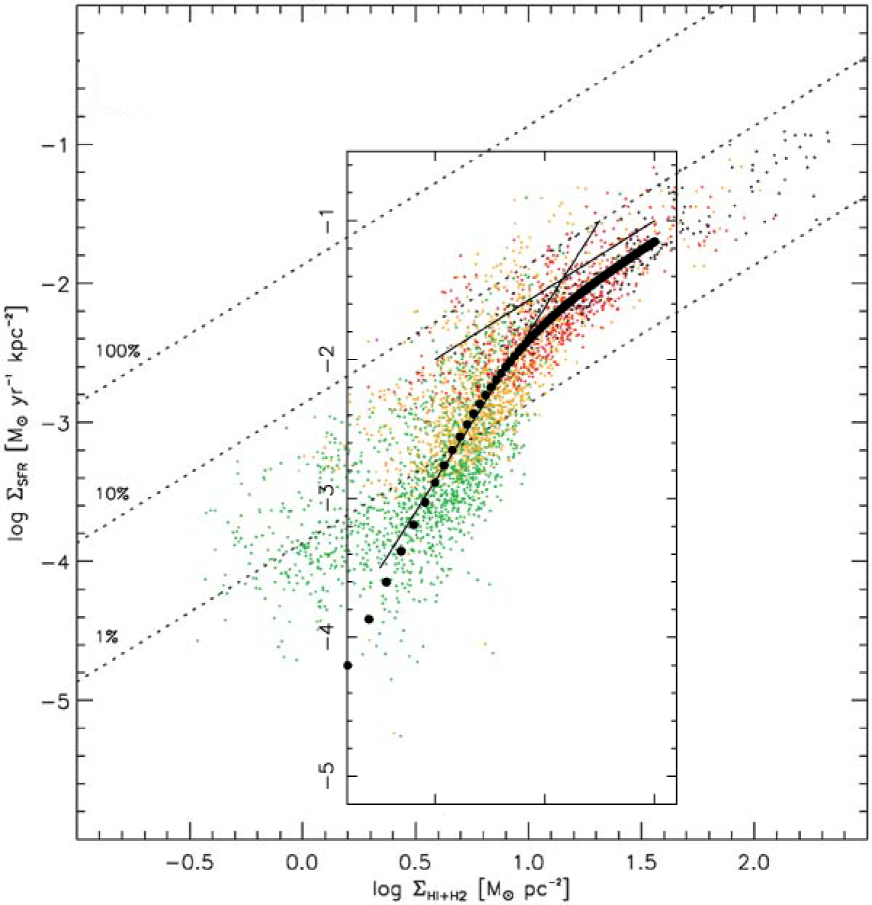
Figure 1: The rate of star formation $\Sigma_{SFR}$ versus total gas (molecular + neutral hydrogen) surface density $\Sigma_{H_{2}+HI}$ for sub-kiloparsec sampled galaxies in Bigiel et al (2008), with the appropriately normalized prediction from Equation 1 superimposed on his Figure 8. The asymptotic linear (unit slope) behavior predicted by Equation 1 is seen at high gas surface densities with an increasingly steeper fall-off toward low gas densities. This particular (discretely sampled) solution is for illustrative purposes only; it is chosen as a representative fit to the general trend in the cumulative plot. However, it does show show how the linear regime is approached at high gas surface densities, and in this particular example the solution asymptotically approaches a power law with $n=2.5$ at low gas densities. The dotted lines of unit slope crossing the diagram correspond to the levels of constant star formation efficiency needed to consume 1, 10 and 100% of the gas reservoir in $10^{8}$ years. The data points are color-coded by their respective radial distances scaled by $r_{25}$ (black $<$ 0.25, red 0.25-0.50, orange 0.50-0.75, and green $>$ 0.75). Detailed fits to individual galaxies will be forthcoming.

Sanduleak’s particular technique in his pioneering study was extended to other galaxies and in the process also generalized to different star-formation tracers. For instance, Hartwick (1971) correlated HII region surface densities with neutral hydrogen surface densities for the Local Group galaxy M31, and derived an exponent $n=3.50\pm 0.12$. Madore, van den Bergh & Rogstad (1974) combined the methods of Sanduleak and Hartwick and correlated both star counts and HII regions with HI surface densities across the face of M33. They found differences between between the two tracers as well as differences as a function of radius; the latter, being suggested by them, as being plausibly due to plane thickness variations. They found exponents ranging from $n=0.57$ to $2.57$, depending on the tracer and the radial region considered, with the outer regions showing a steeper dependence. Tosa & Hamajima (1975), Hamajima & Tosa, (1975) followed Hartwick’s lead and also used HII region number densities and correlated these with the available neutral hydrogen surface densities. They found exponents ranging from $n=1.5$ to $3.5$ in 7 galaxies (SMC, LMC, M31, M51, M101, NGC 2403 and NGC 6946). Their analysis again suggested that the relation was a function of radius where in the examples of M31 and M101 the exponent was again found to be larger in the outer regions when compared to the inner disk. More recently, Bigiel et al. (2008) examined the spatially resolved star formation law in 18 nearby galaxies using both UV (GALEX) and IR (Spitzer) data to characterize the on-going star formation, and exploring both molecular, neutral and total hydrogen gas content as control variables. They found that for total gas (surface) densities in excess of 1M_☉ pc^-2 the star formation rate scaled linearly with total gas (i.e., $n=1.0\pm$0.2), but at lower gas surface densities the power law steepens considerably and is widely dispersed (see their composite Figures 10 and 15, and Figure 1 below).

We now proceed to give a physically motivated, analytic expression capturing these facts. It is hoped that with this formulation galaxy evolution modellers will be able to exploit this simple parametric means of predicting star formation rates based on local gas densities.

2 Timescale Arguments

Numerical simulations of star formation, in search of the underlying parameterization of the causal relation between observed gas densities and current star formation rates, were first presented by Madore (1977). There it was pointed out that if the star formation rate was dimensionally decomposed into its native sub-components of a mass and a timescale then the first term naturally scaled directly as the mean density and the latter term, the timescale, would only have to scale as $\rho^{-1/2}$ in order to give $n=1.5$, a value which seemed to be broadly supported by the observations of the time. That is, the star formation rate $f_{SFR}$ = $M_{*}/\tau_{SFR}\propto\rho_{g}/{\rho_{g}}^{-1/2}\propto{\rho_{g}}^{3/2}$. Many gravitationally controlled timescales depend on ${\rho_{g}}^{-1/2}$ so there was some early, but still a posteriori, justification for this particular interpretation.

However gravity is not the only mechanism operating in the production of stars. And so we ask what are the various modes of star formation that might be considered in trying to predict an appropriate timescale for star formation? And what might the controlling parameters be for those different modes? Here we simply enumerate four main modes that appear to be operating, and then we focus our attention primarily on the first, quiescient star formation. Lessons learned here, we believe, can be applied in provisionally parameterizing the other modes of star formation as well.

Four distinct modes of star formation, whose rates are individually determined by independent physics and very different timescales, immediately suggest themselves: (1) a secular timescale $\tau_{c}$ for unforced, that is to say, quiescent star formation across the galaxy in question, regulated primarily by the natural cloud coalescence and collapse timescales, (2) an induced star-formation timescale, $\tau_{d}$, which is determined by quasi-periodic phenomena that are internal to the galaxy, such as density waves, rotating bars, etc., (3) an impulsive star formation timescale, $\tau_{e}$, which is determined by external, and generally aperiodic encounters or collisions with other nearby galaxies or satellites, and finally (4) a flow timescale, $\tau_{f}$, determining the rate of star formation particularly in the nuclear regions of (typically starburst) galaxies, where angular momentum loss mechanisms are probably the rate-limiting factors.

2.1 Quiescent Star Formation

In this Letter we focus exclusively on parameterizing the quiescent mode of star formation. Starting afresh, from dimensional arguments alone we develop a simplified parameterization of the rate of star formation that now captures the essential non-linear form (Bigiel et al. 2008) of the current observational correlations. In the life cycle of gas, from its diffuse state into collapsing clouds, through the phase change called star formation and finally the cloud’s disruption and redispersal before it begins the cycle again, two critical timescales are identified: (1) a cloud coalescence/(re)collapse timescale $\tau_{c}$, characterizing the systematic assembly and/or re-assembly of neutral hydrogen into a molecular cloud and its subsequent development of a dense core, ultimately leading to the observed star formation event, and then (2) a star-formation-induced “stagnation” timescale, $\tau_{s}$, determined by the presence of hot stars and their disruptive interaction with the birth cloud.

Such a characterization involving two independent timescales is not just convenient, it is methodologically required, because what is done observationally amounts to selecting regions that have a given column density of gas and then equating the relative areal frequency of those regions with a relative temporal frequency (i.e., a cumulative timescale or lifetime) for that density. However that cumulative timescale must itself be the sum of two independent timescales, $\tau_{s}$ and $\tau_{c}$, only one of which, $\tau_{c}$, is assumed here to be a function of the gas density; the other timescale, $\tau_{s}$, being a function of stellar astrophysics and gas heating. The argument is that empirically one needs to take observations, which are per force averages over areas, and map them to a theory that involves averages over time. Those regions of fixed surface density that define the areas are either occupied by currently observabale star formation tracers or they are not. The occupied time is the interval over which the most recently formed stars (and stellar physics) control the gas dynamics; the unoccupied time is primarily the cloud assembly and collapse time, where gas density (and more generally gas physics alone) is assumed to be the controling factor. These are two physically distinct and separable processes that have independent timescales; however, it is their sum that enters into the mapping from the time domain to any given, instantaneously observed, spatial coverage.

The stagnation time, $\tau_{s}$, is ultimately a measure of the (wavelength-independent) timescale over which the general presence of ionization fronts, winds, radiation pressure, SNe, and other disrupting effects of the star-formation events influence the gaseous environment, by stalling and otherwise preventing the onset of the next cycle of star formation in that same region. As such $\tau_{s}$ it is not a timescale to be equated with the lifetime of an individual O star or a B star per se, but rather it is a timescale to be associated with “the disruptive presence of stars, and the star formation event in general”. It is associated with stellar lifetimes but it is a single time period for a given region and it will not be a function of wavelength ($H_{\alpha}$, vs FUV) or any given selected tracer (O stars or B stars). The best that can be said is that it will be at least as long as the longest-lived (high-mass) stars and those by-products (i.e., Type II supernovae) that influence the structure of the local medium in a way that they collectively delay the onset of the next re-coalescence and collapse sequence. Some fraction of the stagnation time will also be coupled to the time it takes gas to recombine after being ionized by the HII region, or to cool back down after being shocked by a supernova blast wave, and both of these are admittedly strong ($n^{2}_{e}$) functions of electron density, but since the observed control parameter being considered here is the neutral and/or molecular gas density, to first order, $\tau_{s}$ should be decoupled.

We equate the “star formation rate” $f_{SFR}$, with the mass of recently formed stars $M_{*}$ divided by some characteristic timescale $\tau$ such that $f_{SFR}=M_{*}/\tau$. We now assume some efficiency $\epsilon$ for converting into stars the total available gas mass $M_{g}$, contained in some fixed volume $V$, such that $M_{*}=\epsilon M_{g}=\epsilon V\rho_{g}$. Furthermore we break $\tau$ down into its two rate-limiting timescales, $\tau_{s}$ and $\tau_{c}$, which, as mentioned above, are the star-formation-induced, cloud-disruption timescales and the neutral-to-molecular cloud formation/collapse timescales, respectively. Accordingly,

$$f_{SFR}={M_{*}\over{\tau}}={\epsilon V\rho_{g}\over{(\tau_{s}+\tau_{c})}}$$

$$~{}~{}~{}~{}~{}~{}~{}={A\rho_{g}\over{(\tau_{s}+B(\rho_{g}/\rho_{c})^{-n})}}$$

$$~{}~{}~{}~{}~{}~{}~{}={A\rho_{g}/\tau_{s}\over{(1+(B\rho_{c}^{n}/\tau_{s})\rho_{g}^{-n})}}$$

$$~{}~{}~{}~{}~{}~{}~{}={\alpha\rho_{g}\over{(1+\beta\rho_{g}^{-n})}}\ \ \ \ \ \ \ \ (1)$$

where $A=\epsilon V$, $\alpha=A/\tau_{s}$, $\beta=(B\rho_{c}^{n}\tau_{s})$ and it is assumed that $\tau_{c}=B(\rho_{g}/\rho_{c})^{-n}$.

3 Discussion and Conclusions

The above derivation was made for quiescent star formation, wherein it is implicitly assumed that the rate-limiting timescale behind this particular mode is the coalescence and collapse time of the ambient gas into molecular clouds, which subsequently act as the more immediate sites for star formation. All of the sub-resolution physics and astrophysics of cloud formation and collapse is secreted away in this simple parameterization on the cloud stagnation timescales ($\tau_{s}$) and local gas densities ($\rho^{-n}$). Other modes of star formation of course exist, and because of the very different physics involved, they deserve their own parameterization; but the simple timescale framework should in principle accommodate these other modes as well. The collisionally driven (impulsive) star formation rate $\tau_{c}$ would have a timescale set by the local galaxian environment. The internally driven star formation rates due to density waves would have their timescales $\tau_{D}$ strictly set locally at a given galactocentric radius by 1/$\mid\Omega_{pattern}-\Omega_{rotation}\mid$, where the denominator is the rate of passage of material through the density wave of fixed pattern speed. Finally, one could imagine finding an appropriate timescale $\tau_{E}$ for the transfer of angular momentum regulating the flow of material into the central regions of galaxies where starburst activity then occurs. In any case the simple dimensionality of the proposed parameterization guarantees some measure of success; the novelty is in decoupling and making explicit the star formation tracer’s visibility timescale from the independent assembly/formation/collision timescale.

There are, of course, other proposed parameterizations of star formation rates, many of which are far more bottom-up and physically based rather than the top-down and more phenomenologically motivated approach historically made and adopted here. Dopita has long argued for a “compound” Schmidt Law (e.g. Dopita & Ryder 1994 and references therein) that depends both on local gas density and the total surface density of matter. Silk (1997) argues that the SFR is self-regulated with gravitational instability playing off against supernova heating of the interstellar medium. Tan (2000) suggested that the cloud-cloud collision timescale was the rate-limiting factor for star formation; while Krumhotz & McKee (2005) suggested a simple linear relation holds between the surface density of molecular hydrogen and SFR based on the suggestion that the free-fall time for giant molecular clouds is a largely independent of the cloud mass (Solomon et al. 1987). Li, Mac Low & Klessen (2005) investigated the role played gravitational instabilities controling star formation rates using a three-dimensional, smooth particle hydro code. Simulations by Dobbs & Pringle (2009) simply tie the SFR to the local dynamical timescale of the gas. Finally, Blitz & Rosolowsky (2006 and earlier references therein) suggest that mid-plane pressure is the controling factor in converting HI into its molecular phase and then on to star formation. A detailed comparison of the predictions of some of these models, as well as a number of thresholding scenarios, with the available observations has been given in Leroy et al. (2008) and the interested reader is referred to that paper for a detailed discussion of their relative merits and degrees of success in matching the observations.

The observed rate of star formation is further complicated in the high density nuclear regions of galaxies that are probably not undergoing typical, quiescent star formation that is the main focus of this Letter. At very high column densities, often only found in the nuclear regions of galaxies, the raw correlation of star formation rates with very high gas column densities appears to steepen with respect to the relation found the lower-density main disk. Assuming that the molecular fraction has been properly estimated and/or measured, we have two possible explanations for these observations, both of which may be operating in any given situation. First, the plane thinkness in these inner regions may be playing a factor in increasing the volume gas density without necessarily changing the apparent column density. Adopting a standard (outer disk) Schmidt law would result in the observed upturn in the correlation because of the increased volume gas density and the non-linear response in the production of stars each of which are only measured in projection.

In addition to, or independently of, any plane thickness compression at very high (nuclear) gas densities the same steepening of the observed relation can be easily induced by another plausible effect, beam dilution. If, within the naturally imposed or artificially selected resolution element empirically used to make the star-tracer and gas density correlations, the actual size of the region undergoing star formation is smaller than the beam then, as in the case of the decreasing plane thickness situation above, the appropriate volume density of the region actually undergoing star formation will be much higher in reality than the beam-smeared and diluted column density would suggest. If this is indeed the case, then the observed correlation of star density versus projected gas surface density would steepen, because of the highly non-linear underlying sensitivity of the rate of star formation to volume density.