Abstract

We present 9 new tunes of the $p_{\perp}$-ordered shower and underlying-event model in Pythia 6.4. These “Perugia” tunes update and supersede the older “S0” family. The data sets used to constrain the models include hadronic $Z^{0}$ decays at LEP, Tevatron min-bias data at 630, 1800, and 1960 GeV, Tevatron Drell-Yan data at 1800 and 1960 GeV, and SPS min-bias data at 200, 546, and 900 GeV. In addition to the central parameter set, called “Perugia 0”, we introduce a set of 8 related “Perugia variations” that attempt to systematically explore soft, hard, parton density, and colour structure variations in the theoretical parameters. Based on these variations, a best-guess prediction of the charged track multiplicity in inelastic, non-diffractive minimum-bias events at the LHC is made. Note that these tunes can only be used with Pythia 6, not with Pythia 8. Note: this report was updated in March 2011 with a new set of variations, collectively labelled “Perugia 2011”, that are optimized for matching applications and which also take into account some lessons from the early LHC data. In order not to break the original text, these are described separately in Appendix B. Note 2: a subsequent “Perugia 2012” update is described in Appendix C.

1 Introduction

Perturbative calculations of collider observables (see e.g. [1] for an introduction) rely on two important prerequisites: factorization and infrared (IR) safety. These are the tools that permit us to relate theoretical calculations to detector-level measured quantities, up to corrections of known dimensionality, which can then be suppressed (or enhanced) by appropriate choices of the dimensionful scales appearing in the observable and process under study. However, in the context of the underlying event (UE), say, we are faced with the fact that we do not (yet) have formal factorization theorems for this component — in fact the most naive attempts at factorization can easily be shown to fail [2, 3]. At the same time, not all collider measurements can be made insensitive to the UE at a level comparable to the achievable experimental precision, and hence the extraction of parameters from such measurements acquires an implicit dependence on our modelling of the UE. Further, when considering observables such as track multiplicities, hadronization corrections, or even short-distance quantities if the precision required is very high, we are confronted with observables which may be experimentally well measured, but which are explicitly sensitive to infrared physics.

The Role of Factorization:

Let us begin with factorization. When applicable, factorization allows us to subdivide the calculation of an observable (regardless of whether it is IR safe or not) into a perturbatively calculable short-distance part and an approximately universal long-distance part, the latter of which may be modelled and constrained by fits to data. However, in the context of hadron collisions, the possibilities of multiple perturbative parton-parton interactions and parton rescattering processes explicitly go beyond the factorization theorems so far developed. Part of the problem is that the underlying event may contain short-distance physics of its own, that can be as hard as, or even harder than, the bremsstrahlung emissions associated with the scattering that triggered the event. Hence the conceptual separation into what we think of as “hard-scattering” and “underlying-event” components is not necessarily equivalent to a clean separation in terms of “short-distance” and “long-distance” physics. Indeed, from ISR energies [4] through the SPS [5, 6] to the Tevatron [7, 8, 9, 10, 11], and also in photoproduction at HERA [12], we see evidence of (perturbative) “minijets” in the underlying event, beyond what bremsstrahlung alone appears to be able to account for. It therefore appears plausible that a universal modelling of the underlying event must take into account that the hard-scattering and underlying-event components can involve similar time scales and have a common, correlated evolution. It is in this spirit that the concept of “interleaved evolution” [13] was developed as the cornerstone of the $p_{\perp}$-ordered models [14, 13] in both Pythia 6 [15] and, more recently, Pythia 8 [16], the latter of which now also incorporates a model of parton rescattering [17].

The Role of Infrared Safety:

The second tool, infrared safety, provides us with a class of observables which are insensitive to the details of the long-distance physics. This works up to corrections of order the long-distance scale divided by the short-distance scale to some (observable-dependent) power, typically

$$\mbox{IR Safe Corrections~{}~{}~{}$\propto$~{}~{}~{}}\frac{Q_{\mathrm{IR}}^{2}}{Q_{\mathrm{UV}}^{2}}$$ (1)

where $Q_{\mathrm{UV}}$ denotes a generic hard scale in the problem, and $Q_{\mathrm{IR}}\sim\Lambda_{\mathrm{QCD}}\sim\mathcal{O}(\mathrm{1\ GeV})$. Of course, in minimum-bias, we typically have $Q_{\mathrm{UV}}^{2}\sim Q_{\mathrm{IR}}^{2}$, wherefore all observables depend significantly on the IR physics (or in other words, when IR physics is all there is, then any observable, no matter how carefully defined, depends on it).

Even when a high scale is present, as in resonance decays, jet fragmentation, or underlying-event-type studies, infrared safety only guarantees us that infrared corrections are small, not that they are zero. Thus, ultimately, we run into a precision barrier even for IR safe observables, which only a reliable understanding of the long-distance physics itself can address.

Finally, there are the non-infrared-safe observables. Instead of the suppressed corrections above, such observables contain logarithms

$$\mbox{IR Sensitive Corrections~{}~{}~{}$\propto$~{}~{}~{}}\alpha_{s}^{n}\log^{m}\left(\frac{Q_{\mathrm{UV}}^{2}}{Q_{\mathrm{IR}}^{2}}\right)~{}~{}~{},~{}~{}~{}m\leq 2n~{}~{}~{},$$ (2)

which grow increasingly large as $Q_{\mathrm{IR}}/Q_{\mathrm{UV}}\to 0$. As an example, consider such a fundamental quantity as particle multiplicities; in the absence of nontrivial infrared effects, the number of partons that would be mapped to hadrons in a naïve local-parton-hadron-duality [18] picture would tend logarithmically to infinity as the IR cutoff is lowered. Similarly, the distinction between a charged and a neutral pion only occurs in the very last phase of hadronization, and hence observables that only include charged tracks are always IR sensitive.

Minimum-Bias and the Underlying Event:

Minimum-bias (MB) and Underlying-Event (UE) physics can therefore be perceived of as offering an ideal lab for studying non-factorized and nonperturbative phenomena, with the added benefit of having access to the highest possible statistics in the case of min-bias. In this context there is no strong preference for IR safe over IR sensitive observables; they merely represent two different lenses through which we can view the infrared physics, each revealing different aspects. By far the most important point is that it is in their combination that we achieve a sort of stereo vision, in which infrared safe observables measuring the overall energy flow are simply the slightly averaged progenitors of the spectra and correlations that appear at the level of individual particles. A systematic programme of such studies can give crucial tests of our ability to model and understand these ubiquitous components, and the resulting improved physics models can then be fed back into the modelling of high-$p_{\perp}$ physics.

Starting from early notions such as “KNO scaling” of multiplicity distributions [19], a large number of theoretical and experimental investigations have been brought to bear on what the physics of a generic, unbiased sample of hadron collisions looks like (for a recent review, see, e.g., [20] and references therein). However, in step with the gradual shift in focus over the last two decades, towards higher-$p_{\perp}$ (“maximum-bias”) physics, the field of QCD entered a golden age of perturbative calculations and infrared safety, during which time the unsafe “soft” physics became viewed increasingly as a non-perturbative quagmire, into the depths of which ventured only fools and old men.

From the perspective of the author’s generation, it was chiefly with a comprehensive set of measurements carried out by Rick Field using the CDF detector at the Tevatron [21, 22, 23, 24, 25, 26], that this perception began to change back towards one of a definable region of particle production that can be subjected to rigorous scrutiny in a largely model-independent way, and an ambitious programme of such measurements is now being drawn up for the LHC experiments. In other words, a well-defined experimental laboratory has been prepared, and is now ready for the testing of theoretical models.

Simultaneously with the LHC efforts, it is important to remember that interesting connections are also being explored towards other, related, fields, such as cosmic ray fragmentation (related to forward fragmentation at the LHC) and heavy-ion physics (related to collective phenomena in hadron-hadron interactions). A nice example of this interplay is given, for instance, by the Epos model [27], which originated in the heavy-ion community, but uses a parton-based model as input and whose properties in the context of ultra-high-energy cosmic ray fragmentation are currently being explored [28, 29]. Also methods from the field of numerical optimization are being applied to Monte Carlo tuning (cf., e.g., the Professor [30] and Profit [31] frameworks), and there are tempting connections back to perturbative QCD. Along the latter vein, we believe that by bringing the logarithmic accuracy of perturbative parton shower calculations under better control, there would be less room for playing out ambiguities in the non-perturbative physics against ambiguities on the shower side, and hence the genuine soft physics could also be revealed more clearly. This is one of the main motivations behind the Vincia project [32, 33].

For the present, as part of the effort to prepare for the LHC era and spur more interplay between theorists and experimentalists, we shall here report on a new set of tunes of the $p_{\perp}$-ordered Pythia framework, which update and supersede the older “S0” family [34, 35, 36, 37]. We have focused in particular on the scaling from lower energies towards the LHC (see also [38, 39, 40, 41]) and on attempting to provide at least some form of theoretical uncertainty estimates, represented by a small number of alternate parameter sets that systematically explore variations in some of the main tune parameters. The full set of new tunes have been made available starting from Pythia version 6.4.23 (though some have been available longer; see the Pythia update notes [42] for details).

This concludes a several-year long effort to present the community with an optimized set of parameters that can be used as default settings for the so-called “new” interleaved shower and underlying-event model in Pythia 6. The author’s intention is to now move fully to the development of Pythia 8. We note that the Perugia tunes can unfortunately not be used directly in Pythia 8, since it uses slightly different parton-shower and colour-reconnection models. A separate set of tunes for Pythia 8 are therefore under development, with several already included in the current version 8.1.42 of that generator.

We also present a few distributions that carry interesting information about the underlying physics, updating and complementing those contained in [37, 43]. For brevity, this text only includes a representative selection, with more results available on the web [44, 45].

The main point is that, while any plot of an infrared sensitive quantity represents a complicated cocktail of physics effects, such that any sufficiently general model presumably could be tuned to give an acceptable description observable by observable, it is very difficult to simultaneously describe the entire set. The real game is therefore not to study one distribution in detail, for which a simple fit would in principle suffice, but to study the degree of simultaneous agreement or disagreement over many, mutually complementary, distributions.

2 Procedure

2.1 Manual vs Automated Tuning

Although Monte Carlo models may appear to have a bewildering array of independently adjustable parameters, it is worth keeping at the front of one’s mind that most of these parameters only control relatively small (exclusive) details of the event generation. The majority of the (inclusive) physics is determined by only a few, very important ones, such as, e.g., the value of the strong coupling, in the perturbative domain, and the form of the fragmentation function for massless partons, in the non-perturbative one.

Manual Tuning:

Armed with a good understanding of the underlying model, and using only the generator itself as a tool, a generator expert would therefore normally take a highly factorized approach to constraining the parameters, first constraining the perturbative ones and thereafter the non-perturbative ones, each ordered in a measure of their relative significance to the overall modelling. This factorization, and carefully chosen experimental distributions corresponding to each step, allows the expert to concentrate on just a few parameters and distributions at a time, reducing the full parameter space to manageable-sized chunks. Still, each step will often involve more than one single parameter, and non-factorizable corrections still imply that changes made in subsequent steps can change the agreement obtained in previous ones by a non-negligible amount, requiring additional iterations from the beginning to properly tune the entire generator framework.

Due to the large and varied data sets available, and the high statistics required to properly explore tails of distributions, mounting a proper tuning effort can therefore be quite intensive — often involving testing the generator against the measured data for thousands of observables, collider energies, and generator settings. Although we have not kept a detailed record, an approximate guess is that the generator runs involved in producing the particular tunes reported on here consumed on the order of 1.000.000 CPU hours, to which can be added an unknown number of man-hours. While some of these man-hours were undoubtedly productive, teaching the author more about his model and resulting in some of the conclusions reported on in this paper, most of them were merely tedious, while still disruptive enough to prevent getting much other work done.

The main steps followed in the tuning procedure for the Perugia tunes are described in more detail in section 2.2 below.

Automated Tuning:

As mentioned in the introduction, recent years have seen the emergence of automated tools that attempt to reduce the amount of both computer and manpower required. The number of machine hours can, for instance, be substantially reduced by making full generator runs only for a limited set of parameter points, and then interpolating between these to obtain approximations to what the true generator result would have been for any intermediate parameter point. In the Professor tool [46, 30], which we rely on for our LEP tuning here, this optimization technique is used heavily, so that after an initial (intensive) initialization period, approximate generator results for any set of generator parameters within the sampled space can be obtained without any need of further generator runs. Taken by itself, such optimization techniques could in principle also be used as an aid to manual tuning, but Professor, and other tools such as Profit [31], attempt to go a step further.

Automating the human expert input is of course more difficult (so the experts believe). What parameters to include, in what order, and which ranges for them to consider “physical”? What distributions to include, over which regions, how to treat correlations between them, and how to judge the relative importance, for instance, between getting the right average of an observable versus getting the right asymptotic slope? In the tools currently on the market, these questions are addressed by a combination of input solicited from the generator authors (e.g., which parameters and ranges to consider, which observables constitute a complete set, etc) and the elaborate construction of non-trivial weighting functions that determine how much weight is assigned to each individual bin and to each distribution. The field is still burgeoning, however, and future sophistications are to be expected. Nevertheless, at this point the overall quality of the tunes obtained with automated methods appear to the author to at least be competitive with the manual ones.

2.2 Sequence of Tuning Steps

We have tuned the Monte Carlo in five consecutive steps (abbreviations which we use often below are highlighted in boldface):

1. Final-State Radiation (FSR) and Hadronization (HAD): using LEP data [47, 48]. For most of the Perugia tunes, we take the LEP parameters given by the Professor collaboration [46, 30]. This improves several event shapes and fragmentation spectra as compared to the default settings. For hadronic yields, especially $\phi^{0}$ was previously wrong by more than a factor of 2, and $\eta$ and $\eta^{\prime}$ yields have likewise been improved. For a “HARD” and a “SOFT” tune variation, we deliberately change the re-normalization scale for FSR slightly away from the central Professor value. Also, since the Professor parameters were originally optimized for the $Q^{2}$-ordered parton shower in Pythia, the newest (2010) Perugia tune goes slightly further, by changing the other fragmentation parameters (by order of 5-10% relative to their Professor values) in an attempt to improve the description of high-$z$ fragmentation and strangeness yields reported at LEP [47, 48] and at RHIC [49, 50], relative to the Professor $p_{\perp}$-ordered tuning. The amount of ISR jet broadening (i.e., FSR off ISR) in hadron collisions has also been increased in Perugia 2010, relative to Perugia 0, in an attempt to improve hadron collider jet shapes and rates [51, 52].

2. Initial-State Radiation (ISR) and Primordial $k_{T}$: using the Drell-Yan $p_{\perp}$ spectrum at 1800 and 1960 GeV, as measured by CDF [53] and DØ [54], respectively. Note that we treat the data as fully corrected for photon bremsstrahlung effects in this case, i.e., we compare the measured points to the Monte Carlo distribution of the “original $Z$ boson”. We are aware that this is not a physically meaningful observable definition, but believe it is the closest we can come to the definition actually used for the data points in both the CDF and DØ studies. See [55] for a more detailed discussion of this issue. Again, we deliberately change the renormalization scale for ISR away from its best fit value for the HARD and SOFT variations, by about a factor of 2 in either direction, which does not appear to lead to serious conflict with the data (see distributions below).

3. Underlying Event (UE), Beam Remnants (BR), and Colour Reconnections (CR): using $N_{\mathrm{ch}}$ [56, 57], $dN_{\mathrm{ch}}/dp_{\perp}$ [58, 59], and $\left<p_{\perp}\right>(N_{\mathrm{ch}})$ [59] in min-bias events at 1800 and 1960 GeV, as measured by CDF. Note that the $N_{\mathrm{ch}}$ spectrum extending down to zero $p_{\perp}$ measured by the E735 Collaboration at 1800 GeV [60] was left out of the tuning, since we were not able to consolidate this measurement with the rest of the data. We do not know whether this is due to intrinsic limitations in the modelling (e.g., mismodeling of the low-$p_{\perp}$ and/or high-$\eta$ regions, which are included in the E735 result but not in the CDF one) or to a misinterpretation on our part of the measured observable. Note, however, that the E735 collaboration itself remarks [60] that its results are inconsistent with those reported by UA5 [61, 62] over the entire range of energies where both experiments have data. So far, the early LHC results at 900 GeV appear to be consistent with UA5, within the limited $\eta$ regions accessible to the experiments [63, 64, 65], but it remains important to check the high-multiplicity tail in detail, in as large a phase space region as possible. We also note that there are some discrepancies between the CDF Run-1 [56] and Run-2 [57] measurements at very low multiplicities, presumably due to ambiguities in the procedure used to correct for diffraction. We have here focused on the high-multiplicity tail, which is consistent between the two. Hopefully, this question can also be addressed by comparisons to early low-energy LHC data. Although the 4 main LHC experiments are not ideal for diffractive studies and cannot identify forward protons, it is likely that a good sensitivity can still be obtained by requiring events with large rapidity gaps, where the gap definition would essentially be limited by the noise levels achievable in the electromagnetic calorimeters.

4. Energy Scaling: using $N_{\mathrm{ch}}$ in min-bias events at 200, 546, and 900 GeV, as measured by UA5 [61, 62], and at 630 and 1800 GeV, as measured by CDF [56].

5. The last two steps were iterated a few times.

Remarks on Jet Universality:

Note that the clean separation between the first and second points in the list above assumes jet universality, i.e., that a $Z^{0}$, for instance, fragments in the same way at a hadron collider as it did at LEP. This is not an unreasonable first assumption [66], but since the infrared environment in hadron collisions is characterized by a different (hadronic) initial-state vacuum, by a larger final-state gluon component, and also by simply having a lot more colour flowing around in general, it is still important to check to what precision it holds explicitly, e.g., by measuring multiplicity and $p_{\perp}$ spectra of identified particles, particle-particle correlations, and particle production ratios (e.g., strange to unstrange, vector to pseudoscalar, baryon to meson, etc.) in situ at hadron colliders. We therefore very much encourage the LHC experiments not to blindly rely on the constraints implied by LEP, but to construct and publish their own full-fledged sets of fragmentation constraints using identified particles. This is the only way to verify explicitly to what extent the models extrapolate correctly to the LHC environment, and gives the possibility to highlight and address any discrepancies.

Remarks on Diffraction:

Note also that the modelling of diffraction in Pythia 6 lacks a dedicated modelling of diffractive jet production, and hence we include neither elastic nor diffractive Monte Carlo events in any of our comparisons. This affects the validity of the modelling for the first few bins in multiplicity. Due also to the discrepancy noted above between the two CDF measurements in this region [56, 57], we therefore assigned less importance to these bins when doing the tunes. We emphasize that widespread use of ill-defined terminologies such as “Non-Single Diffractive” (NSD) events without an accompanying definition of what is meant by that terminology at the level of physical observables contributes to the ambiguities surrounding diffractive corrections in present data sets. Since different diffraction models produce different spectra at the observable level, an intrinsic ambiguity is introduced which was not present in the raw data. We strongly encourage future measurements if not to avoid such terminologies entirely then to at least also make data available in a form which is defined only in terms of physical observables, i.e., using explicit cuts, weighting functions, and/or trigger conditions to emphasize the role of one component over another.

Remarks on Observables:

Finally, note that we did not include any explicit “underlying-event” observables in the tuning. Instead, we rely on the large-multiplicity tail of minimum-bias events to mimic the underlying event. A similar procedure was followed for the older “S0” tune [34, 35], which gave a very good simultaneous description of underlying-event physics at the Tevatron. Conversely, Rick Field’s “Tune A” [67, 39] gave a good simultaneous description of minimum-bias data, despite only having been tuned on underlying-event data. Tuning to one and predicting the other is therefore not only feasible but simultaneously a powerful cross-check on the universality properties of the modelling.

Additional important quantities to consider for further model tests and tuning would be event shapes at hadron colliders [68, 52], observables involving explicit jet reconstruction — including so-called “charged jets” [22] (a jet algorithm run on a set of charged tracks, omitting neutral energy), which will have fluctuations in the charged-to-neutral ratio overlaid on the energy flow and therefore will be more IR than full jets, but still less so than individual particles, and “EM jets” (a jet algorithm run on a set of charged tracks plus photons), which basically adds back the $\pi^{0}$ component to the charged jets and hence is less IR sensitive than pure charged jets while still remaining free of the noisy environment of hadron calorimeters — explicit underlying-event, fragmentation, and jet structure (e.g., jet mass, jet shape, jet-jet separation) observables in events with jets [7, 21, 22, 23, 24, 69, 51, 70, 71, 25, 72, 73, 74], photon + jet(s) events (including the important $\gamma$ + 3-jet signature for double-parton interactions [9, 11]), Drell-Yan events [21, 75, 74], and observables sensitive to the initial-state shower evolution in DIS (see, e.g., [38, 76]).

As mentioned above, it is also important that fragmentation models tuned at LEP be tested in situ at hadron colliders. To this effect, single-particle multiplicities and momentum spectra for identified particles such as $K^{0}_{S}$, vector mesons, protons, and hyperons (in units of GeV and/or normalized to a global measure of transverse energy, such as, e.g., the $p_{\perp}$ of a jet when the event is clustered back to a dijet topology) are the first order of business, and particle-particle correlations the second (e.g., how charge, strangeness, baryon number, etc., are compensated as a function of a distance measure and how the correlation strength of particle production varies over the measured phase space region). Again, these should be considered at the same time as less infrared sensitive variables measuring the overall energy flow. We expect a programme of such measurements to gradually develop as it becomes possible to extract more detailed information from the LHC data and note that some such observables, from earlier experiments, have already been included, e.g., in the Rivet framework, see [30], most notably underlying-event observables from the Tevatron, but also recently some fragmentation spectra from RHIC [49, 50]. See also the underlying-event sections in the HERA-and-the-LHC [38], Tevatron-for-LHC [39], and Les Houches write-ups [40]. A complementary and useful guide to tuning has been produced by the ATLAS collaboration in the context of their MC09 tuning efforts [77].

3 Main Features of the Perugia Tunes

Let us first describe the overall features common to all the Perugia tunes, divided into the same main steps as in the outline of the tuning procedure given in the preceding section: 1) final-state radiation and hadronization, 2) initial-state radiation and primordial $k_{T}$, 3) underlying event, beam remnants, and colour reconnections, and 4) energy scaling. Each step will be accompanied by plots to illustrate salient points and by a summary table in appendix A giving the Perugia parameters relevant to that step, as compared to the older Tune S0A-Pro, which serves as our reference. We shall then turn to the properties of the individual tunes in the following section, and finally to extrapolations to the LHC in the last section.

3.1 Final-State Radiation and Hadronization (Table 2)

As mentioned above, we have taken the LEP tune obtained by the Professor group [46, 30] as our starting point for the FSR and HAD parameters for the Perugia tunes. Since we did not perform this part of the tuning ourselves, we treat these parameters almost as fixed inputs, and only a very crude first attempt at varying them was originally made for the Perugia HARD and SOFT variations. This is reflected in the relatively small differences between the FSR and HAD parameters listed in table 2, compared to S0A-Pro which uses the original Professor parameters. (E.g., most of the tunes use the same parameters for the longitudinal fragmentation function applied in the string hadronization process, including the same Lund functions [78] for light quarks and Bowler functions [79] for heavy quarks.) With the most recent Perugia 2010 tune, an effort was made to manually improve jet shapes, strangeness yields, and high-$z$ fragmentation, which is the reason several of the hadronization parameters differ in this tune as well as in its sister tune Perugia K. A more systematic exploration of variations in the fragmentation parameters is certainly a point to return to in the future, especially in the light of the new identified-particle spectra and jet shape data that will hopefully soon be available from the LHC experiments. For the present, we have focused on the the uncertainties in the hadron-collider-specific parameters, as follows.

3.2 Initial-State Radiation and Primordial $\mathbf{k_{T}}$ (Table 3)

Evolution Variable, Kinematics, and Renormalization Scale:

One of the most significant changes when going from the old (virtuality-ordered) to the new ($p_{\perp}$-ordered) ISR/FSR model concerns the Drell-Yan $p_{\perp}$ spectrum. In the old model, when an originally massless ISR parton evolves to become a jet with a timelike invariant mass, then that original parton is pushed off its mass shell by reducing its momentum components. In particular the transverse momentum components are reduced, and hence each final-state emission off an ISR parton effectively removes $p_{\perp}$ from that parton, and by momentum conservation also from the recoiling Drell-Yan pair. Via this mechanism, the $p_{\perp}$ distribution generated for the Drell-Yan pair is shifted towards lower values than what was initially produced.

Compared to data, this appears to effectively cause any tune of the old Pythia framework with default ISR settings — such as Tune A or the ATLAS DC2/“Rome” tune — to predict a too narrow spectrum for the Drell-Yan $p_{\perp}$ distribution, as illustrated by the comparison of Tune A to CDF and DØ data in fig. 1 (left column). (The inset shows the high-$p_{\perp}$ tail which in all cases is matched to $Z+$jet matrix elements, the default in Pythia for both the virtuality- and $p_{\perp}$-ordered shower models.)

CDF
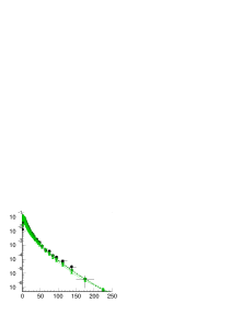
DØ

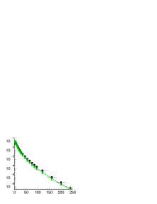
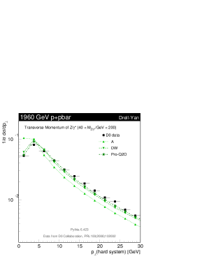
CDF
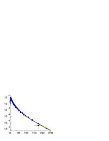
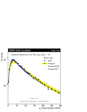
DØ

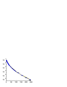
Figure 1: Comparisons to the CDF and DØ measurements of the $p_{\perp}$ of Drell-Yan pairs [53, 54]. Insets show the high-$p_{\perp}$ tails. Left: virtuality-ordered showers. Right: $p_{\perp}$-ordered showers. See [44] for other tunes and collider energies.

We note that a recent theoretical study [80] using virtuality-ordering with a different kinematics map did not find this problem, consistent with our suspicion that it is not the virtuality ordering per se which results in the narrow shape, but the specific recoil kinematics of FSR off FSR in the old shower model.

To re-establish agreement with the measured spectrum without changing the recoil kinematics, the total amount of ISR in the old model had to be increased. This can be accomplished, e.g., by choosing very low values of the renormalization scale (and hence large $\alpha_{s}$ values) for ISR, as illustrated by tunes DW-Pro and Pro-Q2O in fig. 1 (left column). To summarize, the $\alpha_{s}$ choices corresponding to each of the three tunes of the old shower shown in the left pane of fig. 1 are,

$$\begin{array}[]{c}\mbox{{\bf ISR}}\\ \mbox{$Q^{2}$-ordering}\end{array}~{}~{}~{}\left\{\begin{array}[]{rcclll}\mbox{Tune A~{}(100)}&:&\alpha_{s}(p_{\perp}^{2})&~{}\overline{\mathrm{MS}},&\mbox{1-loop},&\Lambda_{\mathrm{CTEQ5L}}\\ \mbox{Tune DW~{}(103)}&:&\alpha_{s}(0.2p_{\perp}^{2})&~{}\overline{\mathrm{MS}},&\mbox{1-loop},&\Lambda_{\mathrm{CTEQ5L}}\\ \mbox{Tune Pro-Q2O~{}(129)}&:&\alpha_{s}(0.14p_{\perp}^{2})&~{}\overline{\mathrm{MS}},&\mbox{1-loop},&\Lambda_{\mathrm{CTEQ5L}}\\ \end{array}\right.~{},$$ (3)

where, for completeness, we have given also the renormalization scheme, loop order, and choice of $\Lambda_{\mathrm{QCD}}$, which are the same for all the tunes.

While the increase of $\alpha_{s}$ nominally reestablishes a good agreement with the Drell-Yan $p_{\perp}$ spectrum, the whole business does smell faintly of fixing one problem by introducing another and hence the defaults in Pythia for these parameters have remained the Tune A ones, at the price of retaining the poor agreement with the Drell-Yan spectrum.

In the new $p_{\perp}$-ordered showers [13], however, FSR off ISR is treated within individual QCD dipoles and does not affect the Drell-Yan $p_{\perp}$. This appears to make the spectrum come out generically much closer to the data, as illustrated by the S0(A) curves in fig. 1 (right column), which use $\alpha_{s}(p_{\perp})$. The only change going to Perugia 0 — which can be seen to be slightly harder — was implementing a translation from the $\overline{\mathrm{MS}}$ definition of $\Lambda$ used previously, to the so-called CMW choice [81] for $\Lambda$, similarly to what is done in Herwig [82, 83].

For both CTEQ5L and CTEQ6L1, the $\Lambda^{\overline{\mathrm{MS}}}_{\mathrm{QCD}}$ value in the PDF set is derived with an LO (1-loop) running of $\alpha_{s}$, which is also what we use in the backwards evolution algorithm in our ISR model. In the Perugia tunes (and also in Pythia by default) we therefore let the $\alpha_{s}$ value for the ISR evolution be determined by the PDF set. The MRST LO* set [84], however, uses an NLO (2-loop) running for $\alpha_{s}$, which gives a roughly 50% larger value for $\Lambda$. Since we do not change the loop order of our ISR evolution, this higher $\Lambda$ value would lead to an increase in, e.g., the mean Drell-Yan $p_{\perp}$ at the Tevatron. In practice, however, this point is obscured by the fact that the LHAPDF interface, used in our code (v.5.8.1), does not return the correct $\Lambda_{QCD}$ value for each PDF set. Instead, a constant value of 0.192 (corresponding to CTEQ5L) is returned. Since we were not aware of this bug in the interface when performing the Perugia tunes, we therefore note that all the tunes are effectively using the CTEQ5L value of $\Lambda$. The pace of evolution with the LO* PDF set is still slightly higher than for CTEQ5L, however. To compensate for this, the renormalization scale was chosen slightly higher for the LO* tune, cf. the PARP(64) values in table 3.

We note that a similar issue afflicted the original CTEQ6L set, which used an NLO $\alpha_{s}$ (with a correspondingly larger value of $\Lambda$). We here use the revised CTEQ6L1 set for our Perugia 6 tune, which uses an LO running and hence should be more consistent with the evolution performed by the shower. Similarly, the LO* set used here could be replaced by the newer LO** one, which uses $p_{\perp}$ instead of $Q^{2}$ as the renormalization scale in $\alpha_{s}$, similarly to what is done in the shower evolution, but this was not yet available at the time our LO* tune was performed. The main reason for sticking to CTEQ5L for Perugia 0 was the desire that this tune can be run with standalone Pythia 6. We note that in Pythia 8, several more recent sets have already been implemented in the standalone version [85], hence removing this restriction from corresponding tuning efforts for Pythia 8. Note also that, since these sets are implemented internally in Pythia 8, the bug in the LHAPDF interface mentioned above does not affect Pythia 8.

Finally, the HARD and SOFT variations shown by the yellow band in the right pane of fig. 1 are obtained by making a variation of roughly a factor of 2 in either direction from the central tune (in the case of the SOFT tune, this is obtained by a combination of reverting to the $\overline{\mbox{MS}}$ value for $\Lambda$ and using $\sqrt{2}p_{\perp}$ as the renormalization scale). In the low-$p_{\perp}$ peak, the HARD variation generates a slightly too broad distribution, but given the large sensitivity of this peak to subleading corrections (see below), we consider this to be consistent with the expected theoretical precision. The $p_{\perp}$ spectrum of the other Perugia tunes will be covered in the section on the individual tunes below.

Phase Space:

A further point concerning ISR that deserves discussion is the phase space over which ISR emissions are allowed. Here, Drell-Yan is a special case, since this process is matched to $Z$+jet matrix elements in Pythia [86, 87], and hence the hardest jet is always described by the matrix element over all of phase space. For unmatched processes which do not contain jets at leading order, the fact that we start the parton shower off from the factorization scale can, however, produce an illusion of almost zero jet activity above that scale. This was studied in [88, 89], where also the consequences of dropping the phase space cutoff at the factorization scale were investigated, so-called power showers. Our current best understanding is that the conventional (“wimpy”) showers with a cutoff at the factorization scale certainly underestimate the tail of ultra-hard emissions while the power showers are likely to overestimate it, hence making the difference between the two a useful measure of uncertainty. Since other event generators usually provide wimpy showers by default, we have chosen to give the power variants as the default in Pythia 6 — not because the power shower approximation is necessarily better, but simply to minimize the risk that an accidental agreement between two generators is taken as a sign of a small overall uncertainty, and also to give a conservative estimate of the amount of hard additional jets that can be expected. Note that a more systematic description of hard radiation that interpolates between the power and wimpy behaviours has recently been implemented in Pythia 8 [90].

For the Perugia models, we have implemented a simpler possibility to smoothly dampen the tail of ultra-hard radiation, using a scale determined from the colour flow as reference. This is done by nominally applying a power shower, but dampening it by a factor

$$P_{\mathrm{accept}}=P_{67}~{}\frac{s_{D}}{4p_{\perp\mathrm{evol}}^{2}}~{},$$ (4)

where $P_{67}$ corresponds to the parameter PARP(67) in the code, $p_{\perp\mathrm{evol}}^{2}$ is the evolution scale for the trial splitting, and $s_{D}$ is the invariant mass of the radiating parton with its colour neighbour, with all momenta crossed into the final state (i.e., it is $\hat{s}$ for annihilation-type colour flows and $-\hat{t}$ for an initial-final connection). This is motivated partly by the desire to give an intermediate possibility between the pure power and pure wimpy options but also partly from findings that similar factors can substantially improve the agreement with final-state matrix elements in the context of the Vincia shower [33]. By default, the Perugia tunes use a value of 1 for this parameter, with the SOFT and HARD tunes exploring systematic variations, see table 3.

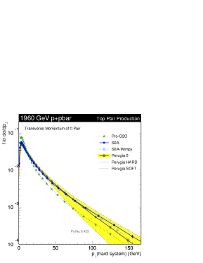
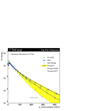
Figure 2: Comparison of new and old tunes for the $p_{\perp}$ of $t\bar{t}$ pairs at the Tevatron (left) and at the LHC at 7 TeV (right). See [44] for other tunes and collider energies.

At the Tevatron, the question of power vs. wimpy showers is actually not much of an issue, since $H/V$+jets is already matched to matrix elements in default Pythia and most other interesting processes either contain QCD jets already at leading order ($\gamma$+jets, dijets, WBF) or have very little phase space for radiation above the factorization scale anyway ($t\bar{t}$, dibosons). This is illustrated by the curves labelled S0A (solid blue) and S0A-Wimpy (dash-dotted cyan) in the left pane of fig. 2, which shows the $p_{\perp}$ spectrum of the $t\bar{t}$ system (equivalent to the Drell-Yan $p_{\perp}$ shown earlier). The two curves do begin to diverge around the top mass scale, but in light of the limited statistics available at the Tevatron, matching to higher-order matrix elements to control this ambiguity does not appear to be of crucial importance. In contrast, when we extrapolate to $pp$ collisions at 7 TeV, shown in the right pane of fig. 2, the increased phase space makes the ambiguity larger. Matching to the proper matrix elements describing the region of jet emissions above $p_{\perp}\sim$ $m_{t}$ may therefore be correspondingly more important, see, e.g., [91]. Note that the extremal Perugia variations span most of the full power/wimpy difference, as desired, while the central ones fall inbetween. Note also that this only concerns the $p_{\perp}$ spectrum of the hard jets — power showers cannot in general be expected to properly capture jet-jet correlations, which are partly generated by polarization effects not accounted for in this treatment.

Primordial $\mathbf{k_{T}}$:

Finally, it is worth remarking that the peak region of the Drell-Yan $p_{\perp}$ spectrum is extremely sensitive to infrared effects. On the experimental side, this means, e.g., that the treatment of QED corrections can have significant effects and that care must be taken to deal with them in a consistent and model-independent manner [55]. On the theoretical side, relevant infrared effects include whether the low-$p_{\perp}$ divergences in the parton shower are regulated by a sharp cutoff or by a smooth suppression (and in what variable), how $\alpha_{s}$ is treated close to the cutoff, and how much “Fermi motion” is given to each of the shower-initiating partons extracted from the protons. A full exploration of these effects probably goes beyond what can meaningfully be studied at the current level of precision. Our models therefore only contain one infrared parameter (in addition to the infrared regularization scale of the shower), called “primordial $k_{T}$”, which should be perceived of as lumping together an inclusive sum of unresolved effects below the shower cutoff. Since the cutoff is typically in the range 1–2 GeV, we do not expect the primordial $k_{T}$ to be much larger than this number, but there is also no fundamental reason to believe it should be significantly smaller. This is in contrast to previous lines of thought, which drew a much closer connection between this parameter and Fermi motion, which is expected to be only a few hundred MeV. In Tune A, the value of primordial $k_{T}$, corresponding to PARP(91) in the code, was originally 1 GeV, whereas it was increased to 2.1 GeV in Tune DW. In the Perugia tunes, it varies in the same range, cf. table 3. Its distribution is assumed to be Gaussian in all the models. Explicit attempts exploring alternative distributions in connection with the write-up of this paper ($1/k_{T}^{6}$ tails and even a flat distribution with a cutoff, see [15, MSTP(91)]) did not lead to significant differences.

3.3 Underlying Event, Beam Remnants, and Colour Reconnections (Table 4)

Charged Multiplicity

The charged particle multiplicity ($N_{\mathrm{ch}}$) distributions for minimum-bias events at 1800 and 1960 GeV at the Tevatron are shown in fig. 3. Particles with $c\tau\geq 10$ mm ($\mu^{\pm}$, $\pi^{\pm}$, $K^{0}_{S}$, $K^{0}_{L}$, $n^{0}$, $\Lambda^{0}$, $\Sigma^{\pm}$, $\Xi^{0}$, $\Xi^{\pm}$, and $\Omega^{\pm}$) are treated as stable. Models include the inelastic, non-diffractive component only.

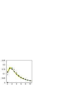
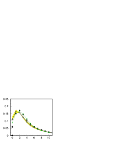
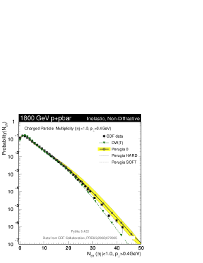
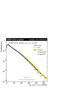
Figure 3: Comparisons to the CDF measurements of the charged track multiplicity at 1800 (left) and 1960 GeV (right) in minimum-bias $p\bar{p}$ collisions. See [44] for other tunes and collider energies.

Note that the Perugia tunes included this data in the tuning, while DW was only tuned to underlying-event data at the same energies. The overall agreement over the many orders of magnitude spanned by these measurements is quite good. On the large-multiplicity tails, DW appears to give a slightly too narrow distribution. In the low-multiplicity peak (see insets), the Perugia tunes fit the 1800 GeV data set better while DW fits the 1960 GeV data set better. As mentioned above, however, diffractive topologies give large corrections in this region, and so the points shown in the insets were not used to constrain the Perugia tunes.

Transverse Momentum Spectrum

The $p_{\perp}$ spectrum of charged particles at 1960 GeV is shown in fig. 4. Note that both plots in the figure show the same data; only the model comparisons are different.

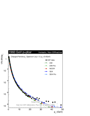
Figure 4: Comparisons to the CDF measurement of the charged particle $p_{\perp}$ spectrum in minimum-bias $p\bar{p}$ collisions at 1960 GeV for two sets of models. See [44] for other tunes and collider energies.

The plot in the left-hand pane illustrates a qualitative difference between the $Q^{2}$- and $p_{\perp}$-ordered models. Comparing DW to NOCR (a tune of the $p_{\perp}$-ordered model which does not employ colour reconnections) we see that the $p_{\perp}$ spectrum is generically slightly harder in the new model than in the old one. Colour reconnections, introduced in S0A, then act to harden this spectrum slightly more, to the point of marginal disagreement with the data. Finally, when we include the Professor tunes to LEP data, nothing much happens to this spectrum in the old model — compare DW with DW-Pro — whereas the spectrum becomes yet harder in the new one, cf. S0A-Pro, now reaching a level of disagreement with the data that we have to take seriously. Since the original spectrum out of the box — represented by NOCR — was originally quite similar to that of DW and DW-Pro, our tentative conclusion is that either the revised LEP parameters for the $p_{\perp}$-ordered shower have some hidden problem and/or the colour reconnection model is hardening the spectrum too much. For the Perugia tunes, we took the latter interpretation, since we did not wish to alter the LEP tuning. Using a modified colour-reconnection model that suppresses reconnections among high-$p_{\perp}$ string pieces (to be described below), the plot in the right-hand pane illustrates that an acceptable level of agreement with the data has been restored in the Perugia tunes, without modifying the Professor LEP parameters.

For completeness we should also note that there are indications of a significant discrepancy developing in the extreme tail of particles with $p_{\perp}>30$ GeV, where all the models fall below the data, a trend that was confirmed with higher statistics in [92]. This discrepancy also appears in the context of NLO calculations folded with fragmentation functions [93], so is not a feature unique to the Pythia modelling. Though we shall not comment on possible causes for this behaviour here (see [94, 95] for a critical assessment), the extreme tail of the $p_{\perp}$ distribution should therefore be especially interesting to check when high-statistics data from the LHC become available.

$\left<p_{\perp}\right>(N_{\mathrm{ch}})$ and Colour Reconnections

While the multiplicity and $p_{\perp}$ spectra are thus, separately, well described by Tune DW, it does less well on their correlation, $\left<p_{\perp}\right>(N_{\mathrm{ch}})$, as illustrated by the plot in the left-hand pane of fig. 5. Since the S0 family of tunes were initially tuned to Tune A, in the absence of published data, the slightly smaller discrepancy exhibited by Tune A carried over to the S0 set of tunes, as illustrated by the same plot. Fortunately, CDF Run-2 data has now been made publicly available [59], corrected to the particle level, and hence it was possible to take the actual data into consideration for the Perugia tunes, resulting in somewhat softer particle spectra in high-multiplicity events, cf. the right-hand pane in fig. 5.

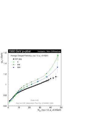
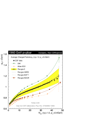
Figure 5: Comparisons to the CDF Run II measurement of the average track $p_{\perp}$ as a function of track multiplicity in min-bias $p\bar{p}$ collisions. Left: The older generation of tunes. Right: the Perugia variations compared to two older tunes. See [44] for other tunes and collider energies.

What is more interesting is how this correlation is achieved by the models. Also shown in the right-hand pane of fig. 5 are comparisons to an older ATLAS tune which did not use the enhanced final-state colour connections that Tunes A and DW employ. A special Perugia variation without colour reconnections, Perugia NOCR, is also shown, and one sees that both this and the ATLAS tune predict too little correlation between $\left<p_{\perp}\right>$ and $N_{\mathrm{ch}}$.

This distribution therefore appears to be sensitive to the colour structure of the events, at least within the framework of the Pythia modelling [96, 34, 35, 36]. The Perugia tunes all (with the exception of NOCR) rely on an infrared toy model of string interactions [34] to drive the increase of $\left<p_{\perp}\right>$ with $N_{\mathrm{ch}}$. The motivation for a model of this type comes from arguing that, in the leading-colour limit used by Monte Carlo event generators, and in the limit of many perturbative parton-parton interactions, the central rapidity region in hadron-hadron collisions would be criss-crossed by a very large number of QCD strings; naïvely one string per perturbative $t$-channel quark exchange, and two per gluon exchange. However, since the actual number of colours is only three, and since the strings would have to be rather closely packed in spacetime, it is not unreasonable to suppose either that the colour field collapses in a more economical configuration already from the start, or that the strings undergo interactions among themselves, before the fragmentation process is complete, that tend to minimize their total potential energy, as given by the area law of classical strings. The toy models used by both the S0 and Perugia tunes do not address the detailed dynamics of this process, but instead employ an annealing-like minimization of the total potential energy, where the string-string interaction strength was originally the only variable parameter [34]. While this gave a reasonable agreement with $\left<p_{\perp}\right>(N_{\mathrm{ch}})$, it still tended to give slightly too hard a tail on the single-particle $p_{\perp}$ distribution, as compared to the Tevatron Run 2 measurement. Therefore, a suppression of reconnections among very high-$p_{\perp}$ string pieces was introduced, reasoning that very fast-moving string systems should be able to more easily “escape” the mayhem in the central region. (Similarly, one could argue that string systems produced in the decay of massive particles with finite lifetimes, such as narrow BSM or Higgs resonances, or even possibly hadronic $t$ or $W$ decays, should be able to escape more easily. We have not so far built in such a suppression, however.)

The switch MSTP(95) controls the choice of colour-reconnection model. In the “S0” model corresponding to MSTP(95)=6 (and =7 to apply it also in lepton collisions), the total probability for a string piece to survive the annealing and preserve its original colour connections is

$$\mbox{{MSTP(95)~{}=~{}6,~{}7~{}~{}~{}:~{}~{}~{}}}P_{\mathrm{keep}}=(1-\zeta P_{78})^{n_{\mathrm{int}}}~{},$$ (5)

where $P_{78}$ corresponds to the parameter PARP(78) in the code and sets the overall colour-reconnection strength and $n_{\mathrm{int}}$ is the number of parton-parton interactions in the current event, giving a rough first estimate of the number of strings spanned between the remnants. (It is thus more likely for a string piece to suffer “colour amnesia” in a busy event, than in a quiet one.) $\zeta$ was introduced together with the Perugia tunes and gives a possibility to suppress reconnections among high-$p_{\perp}$ string pieces,

$$\zeta=\frac{1}{1+P_{77}^{2}\left<p_{\perp}\right>^{2}}~{},$$ (6)

with $P_{77}$ corresponding to PARP(77) in the code and $\left<p_{\perp}\right>$ being a measure of the average transverse momentum per pion that the string piece would produce, $n_{\pi}\propto\ln(s/m_{\pi}^{2})$, with a normalization factor absorbed into $P_{77}$.

Starting from Pythia 6.4.23, a slightly more sophisticated version of colour annealing was introduced, via MSTP(95)=8 (and =9 to apply it also in lepton collisions), as follows. Instead of using the number of multiple parton-parton interactions to give an average idea of the total number of strings between the remnants, the algorithm instead starts by finding a thrust axis for the event (which normally will coincide with the $z$ axis for hadron-hadron collisions). It then computes the density of string pieces along that axis, rapidity-interval by rapidity-interval, with a relatively fine binning in rapidity. Finally, it calculates the reconnection probability for each individual string piece by using the average string density in the region spanned by that string piece, instead of the number of multiple interactions, in the exponent in the above equation:

$$\mbox{{MSTP(95)~{}=~{}8,~{}9~{}~{}~{}:~{}~{}~{}}}P=(1-\zeta P_{78})^{\left<n_{s}\right>(y_{1},y_{2})}~{},$$ (7)

where $\left<n_{s}\right>(y_{1},y_{2})$ is the average number of other string pieces, not counting the piece under consideration, in the rapidity range spanned by the two endpoints of the piece, $y_{1}$ and $y_{2}$. Obviously, the resulting model is still relatively crude — it still has no explicit space-time picture and hence will not generate more subtle effects such as (elliptical) flow, no detailed dynamics model, and no suppression mechanism for reconnections involving long-lived resonances — but at least the reconnection probability has been made a more local function of the actual string environment, which also provides a qualitative variation on the previous models that can be used to explore uncertainties. In the code, the “S0” type is also referred to as the “Seattle” model, since it was written while on a visit there. The newer one is referred to as the “Paquis” type, for similar reasons.

Underlying Event

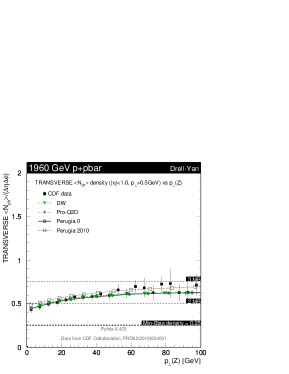
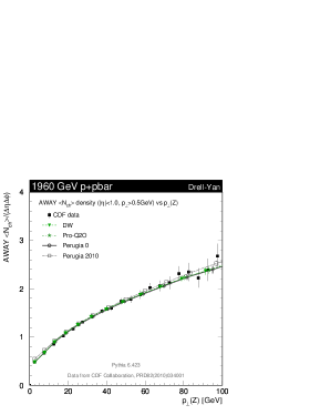
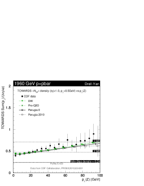
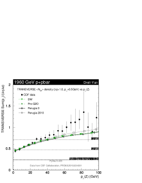
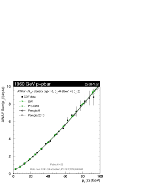
Figure 6: Comparisons to the CDF measurements [75, 74] of the charged particle multiplicity (top row) and $p_{\perp}$ (bottom row) densities in the “TOWARDS” (left), “TRANSVERSE” (middle), and “AWAY” (right) regions of Drell-Yan production at 1960 GeV, as a function of the Drell-Yan $p_{\perp}$.

In fig. 6, we show the $\left<N_{ch}\right>$ density (top row) and the $\left<p_{\perp\mathrm{Sum}}\right>$ density (bottom row) in each of the TOWARDS, TRANSVERSE, and AWAY regions, for Drell-Yan production at the Tevatron, compared to CDF data [75, 74]. The invariant mass window for the lepton pair for this measurement is $70<m_{\ell^{+}\ell^{-}}<110$, in GeV. Tracks with $p_{T}>0.5$ GeV inside $|\eta|<1$ were included, with the same definition of stable charged tracks as above. The leptons from the decaying boson were not included.

The agreement between the Perugia min-bias tunes and data is at the same level as that of more dedicated UE tunes, here represented by DW and Pro-Q2, supporting the assertion made earlier concerning the good universality properties of the Pythia modelling. We note also that the Perugia 2010 variation agrees slightly better with the data in the TRANSVSERSE region, where it has a bit more activity than Perugia 0 does.

Transverse Mass Distribution and MPI Showers

Finally, the old framework did not include showering off the MPI in- and out-states. The new framework does include such showers, which furnish an additional fluctuating physics component. Relatively speaking, the new framework therefore needs less fluctuations from other sources in order to describe the same data. This is reflected in the tunes of the new framework generally having a less lumpy proton (smoother proton transverse density distributions) and fewer total numbers of MPI than the old one. This is illustrated in fig. 7, where a double-logarithmic scale has been chosen in order to reveal the asymptotic behaviour more clearly.

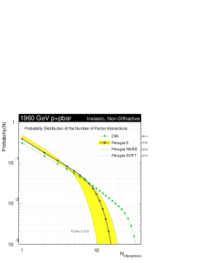
Figure 7: Double-logarithmic plot of the probability distribution of the number of parton-parton interactions in min-bias collisions at the Tevatron, showing that the Perugia tunes obtain the same multiplicity distribution, fig. 3, with fewer MPI than Tune A. See [44] for other tunes and collider energies.

Note that, e.g., for Tune A, the plot shows that more than a per mille of min-bias events have over 30 perturbative parton-parton interactions per event at the Tevatron. This number is reduced by a factor of 2 to 3 in the new models, while the average number of interactions, indicated on the r.h.s. of the plot, goes down by slightly less.

The showers off the MPI also lead to a greater degree of decorrelation and $p_{\perp}$ imbalance between the minijets produced by the underlying event, in contrast to the old framework where these remained almost exactly balanced and back-to-back. This should show up in minijet $\Delta\phi_{jj}$ and/or $\Delta R_{jj}$ distributions sensitive to the underlying event, such as in $Z/W$+multijets with low $p_{\perp}$ cuts on the additional jets. It should also show up as a relative enhancement in the odd components of Fourier transforms of $\phi$ distributions à la [97].

Long-Range Correlations

Further, since showers tend to produce shorter-range correlations than MPI, the new tunes also exhibit smaller long-range correlations than did the old models. That is, if there is a large fluctuation in one end of the detector, it is less likely in the new models that there is a large fluctuation in the same direction in the other end of the detector. The impact of this on the overall modelling, and on correction procedures derived from it, has not yet been studied in great detail. One variable which can give direct experimental information on the correlation strength over both short and long distances is the so-called forward-backward correlation, $b$, defined as in [96, 98]

$$b(\eta_{F})=\frac{\left<n_{F}n_{B}\right>-\left<n_{F}\right>^{2}}{\left<n_{F}^{2}\right>-\left<n_{F}\right>^{2}~{}}~{},$$ (8)

where $n_{F}$ and $n_{B}$ are the number of tracks (or a calorimetric measure of energy deposition) in a pseudorapidity bin centred at $\eta_{F}$ and $\eta_{B}=-\eta_{F}$, respectively, for a given event. The averages indicate averaging over the number of recorded events. The resulting correlation strength, $b$, can be plotted either as a function of $\eta_{F}$ or as a function of the distance, $\Delta\eta$, between the bins.

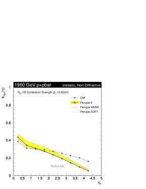
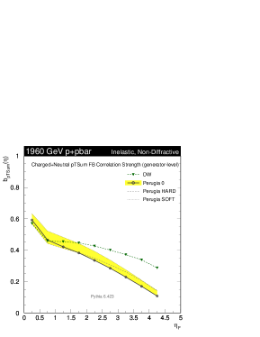
Figure 8: Forward-Backward correlation strengths at the Tevatron in (left) charged particles and (right) charged plus neutral transverse-momentum sum at generator level. See [44] for other tunes and collider energies.

A comparison of the main Perugia tunes to Tune DW is shown in fig. 8, for two different variants of the correlation strength: the plot on the left only includes charged particles with $p_{\perp}>0.4$ GeV and the other (right) includes all energy depositions (charged plus neutral) that would be recorded by an idealized calorimeter. Since estimating the impact on the latter of a real (noisy) calorimeter environment would go beyond the scope of this paper, we here present the correlation at generator level. For the former, we show the behaviour out to $\eta=5$ although the CDF and DØ detectors would of course be limited to measuring it inside the region $|\eta|<1.0$. Note that a measurement of this variable would also be a prerequisite for combining the $dN/d\eta$ measurements from negative and positive $\eta$ regions to form $dN/d|\eta|$, with the proper correlations taken into account. This particular application of the $b$ measurement would require a measurement of $b$ with the same bin sizes as used for $dN/d\eta$. Since the amount of correlation depends on the bin size used (smaller bin sizes are more sensitive to uncorrelated fluctuations), we would advise to perform the $b$ measurement using several different bin sizes, ranging from a very fine binning (e.g., paralleling that of the $dN/d\eta$ measurement), to very wide bins (e.g., one unit in pseudorapidity as used in [96]). For our plots here, we used an intermediate-sized binning of 0.5 units in pseudorapidity.

3.4 Energy Scaling (Table 4)

A final difference with respect to the older S0(A) family of tunes is that we here include data from different colliders at different energies, in an attempt to fix the energy scaling better.

The energy scaling of min-bias and underlying-event phenomena, in both the old and new Pythia models, is driven largely by a single parameter, the scaling power of the infrared regularization scale for the multiple parton interactions, $p_{\perp 0}$, see, e.g., [96, 14, 15]. This parameter is assumed to scale with the collider CM energy squared, $s$, in the following way,

$$p_{\perp 0}^{2}(s)=p_{\perp 0}^{2}(s_{\mathrm{ref}})\left(\frac{s}{s_{\mathrm{ref}}}\right)^{P_{90}}~{},$$ (9)

where $p_{\perp 0}^{2}(s_{\mathrm{ref}})$ is the IR regularization scale given at a specific reference $s=s_{\mathrm{ref}}$, and $P_{90}$ sets the scaling away from $s=s_{\mathrm{ref}}$. In the code, $p_{\perp 0}^{2}(s_{\mathrm{ref}})$ is represented by PARP(82), $\sqrt{s}_{\mathrm{ref}}$ by PARP(89), and $P_{90}$ by PARP(90). Note that large values of $P_{90}$ produce a slower rate of increase in the overall activity with collider energy than low values, since the generation of additional parton-parton interactions in the underlying event is suppressed below $p_{\perp 0}$.

The default value for the scaling power in Pythia 6.2 was $P_{90}=0.16$, motivated [96] by relating it to the scaling of the total cross section, which grows like $\propto E_{\mathrm{cm}}^{0.16}$. When comparing to Tevatron data at 630 GeV, Rick Field found that this resulted in too little activity at that energy, as illustrated in the top row of fig. 9, where tune DWT uses the old default scaling away from the Tevatron and DW uses Rick Field’s value of $P_{90}=0.25$. (The total cross section is still obtained from a Donnachie-Landshoff fit [99] and is not affected by this change.)

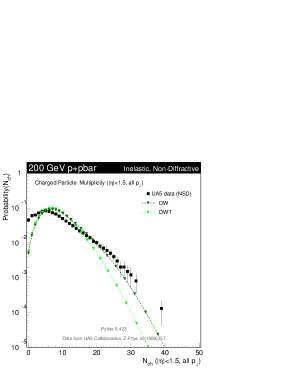
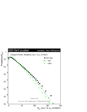
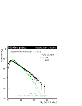
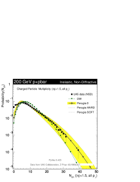
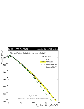
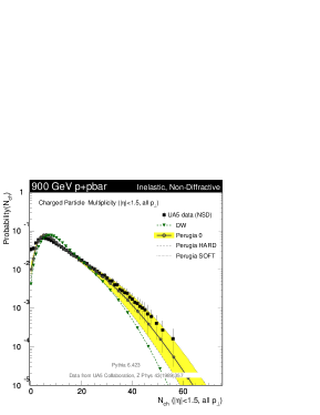
Figure 9: Comparisons to UA5 and CDF measurements of the charged track multiplicity in minimum-bias $p\bar{p}$ collisions at 200 GeV (left), 630 GeV (middle), and 900 GeV (right). Top: Rick Field’s tunes DW and DWT. Bottom: the main Perugia variations compared to DW. See [44] for other tunes and collider energies.

Note that the lowest-multiplicity bins of the UA5 data in particular and the first bin of the CDF data were ignored for our comparisons here, since these contain a large diffractive component, which has not been simulated in the model comparisons.

For the Perugia tunes, the main variations of which are shown in the bottom row of fig. 9, we find that a large range of values, between $0.22$ and $0.32$, can be accommodated without ruining the agreement with the available data, with Perugia 0 using $0.26$.

The energy scaling is therefore still a matter of large uncertainty, and the possibility of getting good additional constraints from the early LHC data is encouraging. The message so far appears to be contradictory, however, with early ATLAS results at 900 GeV [65] appearing to confirm the tendency of the current tunes to undershoot the high-multiplicity tail at 900 GeV (see the right-hand column of fig. 9), which would indicate a slower scaling between 900 and 1800 GeV than what is generated by the models (since they all fit well at 1800 GeV) but preliminary CMS results on the average multiplicity at 2360 GeV [64] indicate the opposite, that the pace of evolution in the models is actually too slow. Furthermore, the CDF data at 630 GeV and the UA5 data at 200 GeV provide additional constraints at lower energies which have made it difficult for us to increase the tail at 900 GeV without coming into conflict with at least one of these other data sets. In view of these tensions, we strongly recommend future studies to include comparisons at different energies.

One issue that can be clearly separated out in this discussion, however, is that the average multiplicity is sensitive to “contamination” from events of diffractive origin, while the high-multiplicity tail is not, and hence a different scaling behaviour with energy (or just a different relative fraction?) of diffractive vs. non-diffractive events may well generate differences between the scaling behaviour of each individual moment of the multiplicity distribution. Attempting to pin down the scaling behaviour moment by moment would therefore also be an interesting possible study. Since the Pythia 6 modelling of diffraction is relatively crude, however, we did not attempt to pursue this question further in the present study, but note that a discussion of whether these tendencies could be given other meaningful physical interpretations, e.g., in terms of low-$x$, saturation, and/or unitarization effects, would be interesting to follow up on.

It should be safe to conclude, however, that there is clearly a need for more systematic examinations of the energy scaling behavior, both theoretically and experimentally, for both diffractive and non-diffractively enhanced event topologies separately. It would also be interesting, for instance, to attempt to separately determine the scaling behaviours for low-activity/peripheral events and for active/central events, e.g., by considering the scaling of the various moments of the multiplicity distribution and by other observables weighted by powers of the event multiplicity.

4 The Perugia Tunes: Tune by Tune

The starting point for all the Perugia tunes, apart from Perugia NOCR, was S0A-Pro, i.e., the original tune “S0” [14, 13, 34, 35], with the Tune A energy scaling (S0A), revamped to include the Professor tuning of flavour and fragmentation parameters to LEP data [46, 30] (S0A-Pro). The starting point for Perugia NOCR was NOCR-Pro. From these starting points, the main hadron collider parameters were retuned to better describe the data sets described above.

As in previous versions, each tune is associated with a 3-digit number which can be given in MSTP(5) as a convenient shortcut. A complete overview of the Perugia tune parameters is given in appendix A and a list of all the predefined tunes that are included with Pythia version 6.423 can be found in appendix E.

Perugia 0 (320):

Uses CTEQ5L parton distributions [100] (the default in Pythia and the most recent set available in the standalone version — see below for Perugia variations using external CTEQ6L1 and MRST LO* distributions). Uses $\Lambda_{\mathrm{CMW}}$ [81] instead of $\Lambda_{\overline{\mathrm{MS}}}$, which results in near-perfect agreement with the Drell-Yan $p_{\perp}$ spectrum, both in the tail and in the peak, cf. fig. 1. Also has slightly less colour reconnections than S0(A), especially among high-$p_{\perp}$ string pieces, which improves the agreement both with the $\left<p_{\perp}\right>(N_{\mathrm{ch}})$ distribution and with the high-$p_{\perp}$ tail of charged particle $p_{\perp}$ spectra, cf [44, dN/dpT (tail)]). Slightly more beam-remnant breakup than S0(A) (more baryon number transport), mostly in order to explore this possibility than due to any necessity of tuning at this point. Without further changes, these modifications would lead to a greatly increased average multiplicity as well as larger multiplicity fluctuations. To keep the total multiplicity unchanged, relative to S0A-Pro, the changes above were accompanied by an increase in the MPI infrared cutoff, $p_{\perp 0}$, which decreases the overall MPI-associated activity, and by a slightly smoother proton mass profile, which decreases the fluctuations. Finally, the energy scaling is closer to that of Tune A (and S0A) than to the old default scaling that was used for S0.

Perugia HARD (321):

A variant of Perugia 0 which has a higher amount of activity from perturbative physics and counter-balances that partly by having less particle production from nonperturbative sources. Thus, the $\Lambda_{{\mathrm{CMW}}}$ value is used for ISR, together with a renormalization scale for ISR of $\mu_{R}=\frac{1}{2}p_{\perp}$, yielding a comparatively hard Drell-Yan $p_{\perp}$ spectrum, cf. the dashed curve labeled “HARD” in the right pane of fig. 1. It also has a slightly larger phase space for both ISR and FSR, uses higher-than-nominal values for FSR, and has a slightly harder hadronization. To partly counter-balance these choices, it has less “primordial $k_{T}$”, a higher IR cutoff for the MPI, and more active colour reconnections, yielding a comparatively high curve for $\left<p_{\perp}\right>(N_{\mathrm{ch}})$, cf. fig. 5. Warning: this tune has more ISR but also more FSR. The final number of reconstructed jets may therefore not appear to change very much, and if the number of ISR jets is held fixed (e.g., by matching), this tune may even produce fewer events, due to the increased broadening. For a full ISR/FSR systematics study, the amount of ISR and FSR should be changed independently.

Perugia SOFT (322):

A variant of Perugia 0 which has a lower amount of activity from perturbative physics and makes up for it partly by adding more particle production from nonperturbative sources. Thus, the $\Lambda_{\overline{\mathrm{MS}}}$ value is used for ISR, together with a renormalization scale of $\mu_{R}=\sqrt{2}p_{\perp}$, yielding a comparatively soft Drell-Yan $p_{\perp}$ spectrum, cf. the dotted curve labeled “SOFT” in the right pane of fig. 1. It also has a slightly smaller phase space for both ISR and FSR, uses lower-than-nominal values for FSR, and has a slightly softer hadronization. To partly counter-balance these choices, it has a more sharply peaked proton mass distribution, a more active beam remnant fragmentation, a slightly lower IR cutoff for the MPI, and slightly less active colour reconnections, yielding a comparatively low curve for $\left<p_{\perp}\right>(N_{\mathrm{ch}})$, cf. fig. 5. Again, a more complete variation would be to vary the amount of ISR and FSR independently, at the price of introducing two more variations (see above). We encourage users that desire a complete ISR/FSR systematics study to make these additional variations on their own.

Perugia 3 (323):

A variant of Perugia 0 which has a different balance between MPI and ISR and a different energy scaling. Instead of a smooth dampening of ISR all the way to zero $p_{\perp}$, this tune uses a sharp cutoff at 1.25 GeV, which produces a slightly harder ISR spectrum. The additional ISR activity is counter-balanced by a higher infrared MPI cutoff. Since the ISR cutoff is independent of the collider CM energy in this tune, the multiplicity would nominally evolve very rapidly with energy. To offset this, the MPI cutoff itself must scale very quickly, hence this tune has a very large value of the scaling power of that cutoff. This leads to an interesting systematic difference in the scaling behavior, with ISR becoming an increasingly more important source of particle production as the energy increases in this tune, relative to Perugia 0. This is illustrated in fig. 10, where we show the scaling of the min-bias charged multiplicity distribution and the Drell-Yan $p_{\perp}$ spectrum between the Tevatron (left) and the LHC at 14 TeV (right).

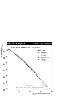
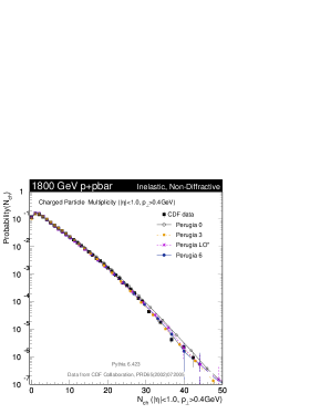
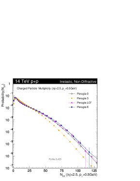
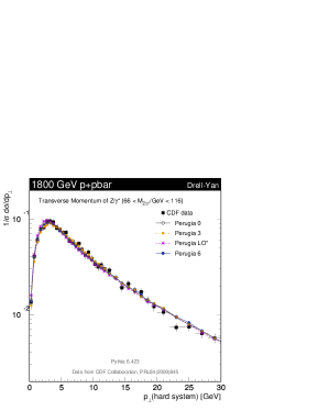
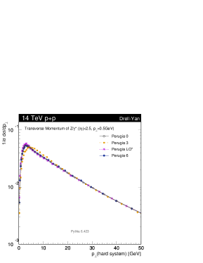
Figure 10: Charged particle multiplicity and Drell-Yan $p_{\perp}$ spectra at the Tevatron (left) and at the LHC at 14 TeV (right) for the Perugia 0, 3, LO*, and 6 tunes. In particular, the Perugia 3 curve on the lower right-hand plot illustrates the consequences of choosing a different regularization procedure for ISR in the infrared, which shifts the position of the infrared peak of the Drell-Yan $p_{\perp}$ spectrum without affecting the tail of the distribution.

One sees that, while the overall multiplicity grows less fast with energy in Perugia 3, the position of the soft peak in Drell-Yan becomes harder, reflecting the relative increase in ISR, despite the decrease in MPI.

Perugia NOCR (324):

An update of NOCR-Pro that attempts to fit the data sets as well as possible, without invoking any explicit colour reconnections. Can reach an acceptable agreement with most distributions, except for the $\left<p_{\perp}\right>(N_{\mathrm{ch}})$ one, cf. fig. 5. Since there is a large amount of “colour disturbance” in the remnant, this tune gives rise to a very large amount of baryon number transport, even greater than for the SOFT variant above.

Perugia X (325):

A Variant of Perugia 0 which uses the MRST LO* PDF set [84]. Due to the increased gluon densities, a slightly lower ISR renormalization scale and a higher MPI cutoff than for Perugia 0 is used. Note that, since we are not yet sure the implications of using LO* for the MPI interactions have been fully understood, this tune should be considered experimental for the time being. In fig. 10, we see that the choice of PDF does not greatly affect neither the min-bias multiplicity nor the Drell-Yan $p_{\perp}$ distribution, once the slight retuning has been done. Thus, this tune is not intended to differ significantly from Perugia 0, but only to allow people to explore the LO* set of PDFs without ruining the tuning. See [44, Perugia PDFs] for more distributions.

Perugia 6 (326):

A Variant of Perugia 0 which uses the CTEQ6L1 PDF set [101]. Identical to Perugia 0 in all other respects, except for a slightly lower MPI infrared cutoff at the Tevatron and a lower scaling power of the MPI infrared cutoff (in other words, the CTEQ6L1 distributions are slightly lower than the CTEQ5L ones, on average, and hence a lower regularization scale can be tolerated). The predictions obtained are similar to those of Perugia 0, cf., e.g., fig. 10 and [44].

Perugia 2010 (327):

A variant of Perugia 0 with the amount of FSR outside resonance decays increased to agree with the level inside them (specifically the Perugia-0 value for hadronic $Z$ decays at LEP is used for FSR also outside $Z$ decays in Perugia 2010, where Perugia 0 uses the lower $\alpha_{s}$ value derived from the PDFs instead), in an attempt to bracket the description of hadronic event shapes relative to the comparison of Perugia 0 to NLO+NLL resummations in [52] and also to improve the description of jet shapes [51]. The total strangeness yield has also been increased, since the original parameters, tuned by Professor, were obtained for the $Q^{2}$-ordered shower and small changes were observed when going to the $p_{\perp}$-ordered ones. High-$z$ fragmentation has been modified by a slightly larger infrared cutoff, which hardens the fragmentation spectrum slightly. The amount of baryon number transport has been increased slightly, mostly in order to explore the consequences of the junction fragmentation framework better, and the colour reconnection model has been changed to the newest one, MSTP(95)=8. See [44] for plots using this tune.

Perugia K (328):

A variant of Perugia 2010 that introduces a “$K$” factor on the QCD $2\to 2$ scattering cross sections used in the multiple-parton-interaction framework. The $K$-factor applied is set to a constant value of 1.5. This should make the underlying event more “jetty” and pushes the underlying-event activity towards higher $p_{\perp}$. To compensate for the increased activity at higher $p_{\perp}$, the infrared regularization scale is larger for this tune, cf. table 4 in appendix A. It does not give an extremely good central fit to all data, but represents a theoretically interesting variation to explore.

The Perugia 2011 Tunes (350-359):

The 2011 updates of the Perugia tunes were not included in the original published version of this manuscript. For reference, a description of them has been included in Appendix B of this updated preprint.

The Perugia 2012 Tunes (370-383):

The 2012 updates of the Perugia tunes were not included in the original published version of this manuscript. For reference, a description of them has been included in Appendix C of this updated preprint.

5 Extrapolation to the LHC

“Predictions”

Part of the motivation for updating the S0 family of tunes was specifically to improve the constraints on the energy scaling to come up with tunes that extrapolate more reliably to the LHC. This is not to say that the uncertainty is still not large, but as mentioned above, it does seem that, e.g., the default Pythia scaling is not able to account for the scaling between the lower-energy data sets, and so this is naturally reflected in the updated parameters.

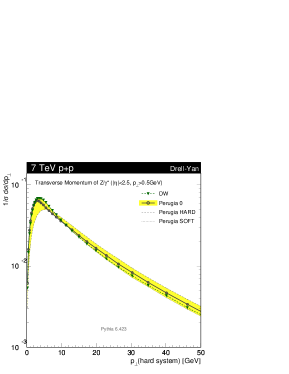
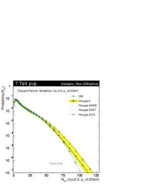
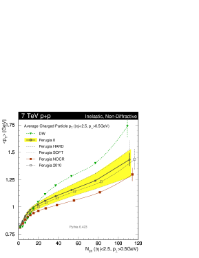
Figure 11: Perugia “predictions” for the $p_{\perp}$ of Drell-Yan pairs (left), the charged track multiplicity in min-bias (center), and the average track $p_{\perp}$ vs. $N_{\mathrm{ch}}$ in min-bias (right) at the LHC at 7 TeV. See [44] for other tunes and collider energies.

In fig. 11, we compare the main Perugia variations to Rick Field’s Tune DW on the Drell-Yan $p_{\perp}$ distribution (using the CDF cuts), the charged track multiplicity distribution in (inelastic, non-diffractive) minimum-bias collisions, and the average track $p_{\perp}$ as a function of multiplicity at the initial LHC center-of-mass energy of 7 TeV. We hope this helps to give a feeling for the kind of ranges spanned by the Perugia tunes (the PDF variations give almost identical results to Perugia 0 for these distributions and are not shown. The Perugia 2010 variation gives the same Drell-Yan $p_{\perp}$ spectrum and is therefore not shown in the left-hand pane). A full set of plots including also the 14 TeV center-of-mass energy, for both the central region, $|\eta|<2.5$, and the region $1.8<\eta<4.9$ covered by LHCb, can be found on the web [44].

However, in addition to these plots, we thought it would be interesting to make at least one set of numerical predictions for an infrared sensitive quantity that could be tested with the very earliest high-energy LHC data. We therefore used the Perugia variations to get an estimate for the mean multiplicity of charged tracks in (inelastic, non-diffractive) minimum-bias $pp$ collisions at center-of-mass energies of 0.9, 2.36, 7, 10, and 14 TeV, as shown in table 1. In order to facilitate comparison with data sets that may include diffraction in the first few multiplicity bins, we recomputed the means with up to the first 4 bins excluded, and model uncertainties were inflated slightly for the first two bins. The uncertainty estimates correspond to roughly twice the largest difference between individual models and only drop below 10% near the collider energies used to constrain the models and then only when the lowest-multiplicity bins are excluded. Note also, however, that the uncertainties nowhere become larger than 20%. This presumably still underestimates the full theoretical uncertainty, due to intrinsic limitations in our ability to vary the models, but we hope nonetheless that it furnishes a useful first estimate.

Predictions for Mean Densities of Charged Tracks (Inelastic, Non-Diffractive Events)
	$\displaystyle\frac{\left<N_{\mathrm{ch}}\right>|_{N_{\mathrm{ch}}\geq 0}}{\Delta\eta\Delta\phi}$	$\displaystyle\frac{\left<N_{\mathrm{ch}}\right>|_{N_{\mathrm{ch}}\geq 1}}{\Delta\eta\Delta\phi}$	$\displaystyle\frac{\left<N_{\mathrm{ch}}\right>|_{N_{\mathrm{ch}}\geq 2}}{\Delta\eta\Delta\phi}$	$\displaystyle\frac{\left<N_{\mathrm{ch}}\right>|_{N_{\mathrm{ch}}\geq 3}}{\Delta\eta\Delta\phi}$	$\displaystyle\frac{\left<N_{\mathrm{ch}}\right>|_{N_{\mathrm{ch}}\geq 4}}{\Delta\eta\Delta\phi}$
LHC 0.9 TeV	$0.21\pm 0.03$	$0.22\pm 0.03$	$0.24\pm 0.02$	$0.26\pm 0.02$	$0.30\pm 0.02$
LHC 2.36 TeV	$0.27\pm 0.03$	$0.28\pm 0.03$	$0.30\pm 0.02$	$0.33\pm 0.02$	$0.36\pm 0.02$
LHC 7 TeV	$0.36\pm 0.04$	$0.37\pm 0.04$	$0.39\pm 0.04$	$0.42\pm 0.05$	$0.46\pm 0.04$
LHC 10 TeV	$0.40\pm 0.05$	$0.41\pm 0.05$	$0.43\pm 0.05$	$0.46\pm 0.06$	$0.50\pm 0.06$
LHC 14 TeV	$0.44\pm 0.06$	$0.45\pm 0.06$	$0.47\pm 0.06$	$0.51\pm 0.06$	$0.54\pm 0.07$

Table 1: Best-guess predictions for the mean density of charged tracks for min-bias $pp$ collisions at several different LHC energies. These numbers should be compared to data corrected to 100% track finding efficiency for tracks with $|\eta|<2.5$ and $p_{\perp}>0.5$ GeV and 0% efficiency outside that region. The definition of a stable particle was set at $c\tau\geq 10$mm (e.g., the two tracks from a $\Lambda^{0}\to p^{+}\pi^{-}$ decay were not counted). The $\pm$ values represent the estimated uncertainty, based on the Perugia tunes. No simulation of diffraction was included in these numbers.

Comparison to the Current LHC Data

At a late stage while preparing this article, data from the initial LHC runs at 900 GeV became available in the HepDATA web repository. We were therefore able to include a comparison of Perugia 0 and a few main variations to the 900 GeV ATLAS data [65]. We here explicitly omit bins with $N_{\mathrm{ch}}<3$ in the multiplicity and $\left<p_{\perp}\right>(N_{\mathrm{ch}})$ distributions since we did not include diffractive events in the simulation. The resulting comparisons are shown in fig. 12.

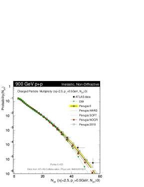
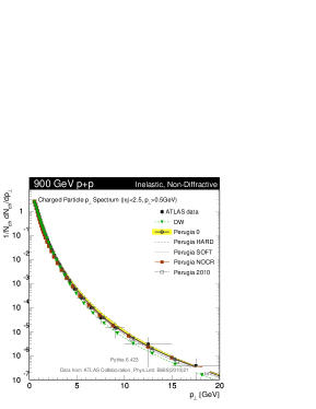
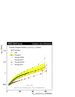
Figure 12: Perugia “predictions” for the charged multiplicity (left), $p_{\perp}$ (center), and $\left<p_{\perp}\right>(N_{\mathrm{ch}})$ distributions in inelastic, non-diffractive $pp$ collisions at 900 GeV, compared with ATLAS data. See [44] for other tunes and collider energies.

The overall agreement between the models and the data is good, which is not surprising given that the 900 GeV beam energy lies well within the energy span inside which the models were tuned. One point that may be worth remarking on is that the models appear to be undershooting the tail of the multiplicity distribution slightly (left). This confirms the tendency already observed in the comparison to the UA5 data, cf. fig. 9 while the models had a tendency to overshoot the tails of the Tevatron distributions, cf. figs. 3 and 9. Combined with early indications at 7 TeV from ALICE [102] and CMS [103] that, likewise, confirm an undershooting by the models of the high-multiplicity tail, we observe that it may be particularly difficult to describe both the Tevatron and LHC data sets simultaneously and that more work in this direction would be fruitful. One way of getting closer to an apples-to-apples comparison in a study of this particular issue would be to perform an LHC measurement applying the same cuts as those used by the CDF min-bias analysis.

6 Conclusions

We have presented a set of updated parameter sets (tunes) for the interleaved $p_{\perp}$-ordered shower and underlying-event model in Pythia 6.4. These parameter sets include the revisions to the fragmentation and flavour parameters obtained by the Professor group [46, 30]. The new sets further include more Tevatron data and more data from different collider CM energies in an attempt to simultaneously improve the overall description of the Tevatron data while also improving the reliability of the extrapolations to the LHC. We have also attempted to deliver a first set of “theoretical uncertainty bands”, by including alternative tunes with systematically different parameter choices. The new tunes are available from Pythia version 6.4.23, via the routine PYTUNE or, alternatively, via the switch MSTP(5).

Our conclusions are that reasonably good overall fits can be obtained, at the 10-20% level, but that the contribution of diffractive processes and the scaling of the overall activity with collider energy are still highly uncertain. Other interesting questions to pursue concern the spectrum of ultra-hard single hadrons with momenta above 30 GeV [59, 93, 92, 94, 95], the (possibly connected) question of collective effects in $pp$ and the dynamics driving such effects, the contribution and properties of diffractive interactions, tests of jet universality by constraining fragmentation models better in situ at hadron colliders as compared to constraints coming from LEP and HERA, and the question of the relative balance between different particle production mechanisms with different characteristics; e.g., between soft beam remnant fragmentation, multiple parton interactions, and traditional parton-shower / radiative corrections to the fundamental scattering processes.

We note that these tunes still only included LEP, Drell-Yan, and minimum-bias data directly, and that the lowest-multiplicity bins of the latter were ignored due to their relatively stronger sensitivity to diffractive physics which we deemed it beyond the scope of this analysis to attack. Furthermore, only one Drell-Yan distribution was used, the inclusive $p_{\perp}$ spectrum. Leading-jet, $V/\gamma$+jet(s), underlying-event and jet structure observables were not considered explicitly. We wish to emphasize that such studies furnish additional important inputs both to tuning and to jet calibration efforts through such observables as jet rates, jet pedestals, jet masses, jet-jet masses (and inter-jet distances), jet profiles, and dedicated jet substructure variables.

We hope these tunes will be useful to the RHIC, Tevatron, and LHC communities.

Acknowledgments

The Perugia tunes derive their names from the Perugia MPI Workshop in 2008, which brought people from different communities together, and helped us take some steps towards finding a common language. We thank the Fermilab computing division, S. Timm in particular, and the Fermilab theory group for providing and maintaining excellent dedicated computing resources without which the large runs necessary for this tuning effort would have been impossible. We acknowledge many fruitful interactions with the RHIC, Tevatron, and LHC experimental communities, and are particularly grateful to B. Cooper, L. Galtieri, B. Heinemann, G. Hesketh, D. Kar, P. Lenzi, A. Messina, and L. Tomkins for detailed counter-checks and feedback. In combination with the writeup of this article, the author agrees to owing Lisa Randall a bottle of champagne if the first published measurement at 10 or 14 TeV of any number in table 1 is outside the range given in the table, and vice versa.

This work was supported in part by the Marie Curie research training network “MCnet” (contract number MRTN-CT-2006-035606) and by the U.S. Department of Energy under contract No. DE-AC02-07CH11359.

Appendix A Parameters for the Perugia Tunes

The following tables give an overview of the parameter settings in Pythia corresponding to the Perugia tunes described in this paper. The settings for the previous “best” tune of the $p_{\perp}$-ordered model, Tune S0A-Pro, are included for reference.

Parameter	Type	S0APro	P0	PHARD	PSOFT	P3	PNOCR	PLO∗	P6	P2010	PK
MSTP(5)	Tune	310	320	321	322	323	324	325	326	327	328
PARJ(81)	FSR	0.257	0.257	0.3	0.2	0.257	0.257	0.257	0.257	0.26	0.26
PARJ(82)	FSR	0.8	0.8	0.8	0.8	0.8	0.8	0.8	0.8	1.0	1.0
MSTJ(11)	HAD	5	5	5	5	5	5	5	5	5	5
PARJ(1)	HAD	0.073	0.073	0.073	0.073	0.073	0.073	0.073	0.073	0.08	0.08
PARJ(2)	HAD	0.2	0.2	0.2	0.2	0.2	0.2	0.2	0.2	0.21	0.21
PARJ(3)	HAD	0.94	0.94	0.94	0.94	0.94	0.94	0.94	0.94	0.94	0.94
PARJ(4)	HAD	0.032	0.032	0.032	0.032	0.032	0.032	0.032	0.032	0.04	0.04
PARJ(11)	HAD	0.31	0.31	0.31	0.31	0.31	0.31	0.31	0.31	0.35	0.35
PARJ(12)	HAD	0.4	0.4	0.4	0.4	0.4	0.4	0.4	0.4	0.35	0.35
PARJ(13)	HAD	0.54	0.54	0.54	0.54	0.54	0.54	0.54	0.54	0.54	0.54
PARJ(21)	HAD	0.313	0.313	0.34	0.28	0.313	0.313	0.313	0.313	0.36	0.36
PARJ(25)	HAD	0.63	0.63	0.63	0.63	0.63	0.63	0.63	0.63	0.63	0.63
PARJ(26)	HAD	0.12	0.12	0.12	0.12	0.12	0.12	0.12	0.12	0.12	0.12
PARJ(41)	HAD	0.49	0.49	0.49	0.49	0.49	0.49	0.49	0.49	0.35	0.35
PARJ(42)	HAD	1.2	1.2	1.2	1.2	1.2	1.2	1.2	1.2	0.9	0.9
PARJ(46)	HAD	1.0	1.0	1.0	1.0	1.0	1.0	1.0	1.0	1.0	1.0
PARJ(47)	HAD	1.0	1.0	1.0	1.0	1.0	1.0	1.0	1.0	1.0	1.0

Table 2: Final-State Radiation and Hadronization Parameters of the Perugia tunes compared to S0A-Pro. For more information on each parameter, see [15].

Parameter	Type	S0APro	P0	PHARD	PSOFT	P3	PNOCR	PLO∗	P6	P2010	PK
MSTP(5)	Tune	310	320	321	322	323	324	325	326	327	328
MSTP(51)	PDF	7	7	7	7	7	7	20650	10042	7	7
MSTP(52)	PDF	1	1	1	1	1	1	2	2	1	1
MSTP(3)	$\Lambda$	2	2	2	2	2	2	2	2	1	1
MSTU(112)	$\Lambda$	-	-	-	-	-	-	-	-	4	4
PARU(112)	$\Lambda$	-	-	-	-	-	-	-	-	0.192	0.192
PARP(1)	ME	-	-	-	-	-	-	-	-	0.192	0.192
PARP(61)	ISR	-	-	-	-	-	-	-	-	0.192	0.192
PARP(72)	IFSR	-	-	-	-	-	-	-	-	0.26	0.26
MSTP(64)	ISR	2	3	3	2	3	3	3	3	3	3
PARP(64)	ISR	1.0	1.0	0.25	2.0	1.0	1.0	2.0	1.0	1.0	1.0
MSTP(67)	ISR	2	2	2	2	2	2	2	2	2	2
PARP(67)	ISR	4.0	1.0	4.0	0.25	1.0	1.0	1.0	1.0	1.0	1.0
PARP(71)	IFSR	4.0	2.0	4.0	1.0	2.0	2.0	2.0	2.0	2.0	2.0
MSTP(70)	ISR	2	2	0	1	0	2	2	2	2	2
PARP(62)	ISR	-	-	1.25	-	1.25	-	-	-	-	-
PARP(81)	ISR	-	-	-	1.5	-	-	-	-	-	-
MSTP(72)	ISR	0	1	1	0	2	1	1	1	2	2
MSTP(91)	BR	1	1	1	1	1	1	1	1	1	1
PARP(91)	BR	2.0	2.0	1.0	2.0	1.5	2.0	2.0	2.0	2.0	2.0
PARP(93)	BR	10.0	10.0	10.0	10.0	10.0	10.0	10.0	10.0	10.0	10.0

Table 3: Parton-Density, Initial-State Radiation, and Primordial $k_{T}$ parameters of the Perugia tunes compared to S0A-Pro. For more information on each parameter, see [15].

Parameter	Type	S0APro	P0	PHARD	PSOFT	P3	PNOCR	PLO∗	P6	P2010	PK
MSTP(5)	Tune	310	320	321	322	323	324	325	326	327	328
MSTP(81)	UE	21	21	21	21	21	21	21	21	21	21
PARP(82)	UE	1.85	2.0	2.3	1.9	2.2	1.95	2.2	1.95	2.05	2.45
PARP(89)	UE	1800	1800	1800	1800	1800	1800	1800	1800	1800	1800
PARP(90)	UE	0.25	0.26	0.30	0.24	0.32	0.24	0.23	0.22	0.26	0.26
MSTP(82)	UE	5	5	5	5	5	5	5	5	5	5
PARP(83)	UE	1.6	1.7	1.7	1.5	1.7	1.8	1.7	1.7	1.5	1.5
PARP(84)	UE	-	-	-	-	-	-	-	-	-	-
MSTP(33)	“K”	0	0	0	0	0	0	0	0	0	10
PARP(32)	“K”	-	-	-	-	-	-	-	-	-	1.5
MSTP(88)	BR	0	0	0	0	0	0	0	0	0	0
PARP(79)	BR	2.0	2.0	2.0	2.0	2.0	2.0	2.0	2.0	2.0	2.0
MSTP(89)	BR	1	1	1	0	1	2	1	1	0	0
PARP(80)	BR	0.01	0.05	0.01	0.05	0.03	0.01	0.05	0.05	0.1	0.1
MSTP(95)	CR	6	6	6	6	6	6	6	6	8	8
PARP(78)	CR	0.2	0.33	0.37	0.15	0.35	0.0	0.33	0.33	0.035	0.033
PARP(77)	CR	0.0	0.9	0.4	0.5	0.6	0.0	0.9	0.9	1.0	1.0

Table 4: Underlying-Event, Beam-Remnant, and Colour-Reconnection parameters of the Perugia tunes compared to S0A-Pro. For more information on each parameter, see [15].

Appendix B The Perugia 2011 Tunes

An update of the Perugia tunes was prepared in the Spring of 2011, with the following main goals,

• Use the same value of $\Lambda_{\mathrm{QCD}}$ for all shower activity (ISR and FSR), in particular to simplify matching applications.

  • The common value is taken from a Professor fit to LEP event shapes and jet rates [46, 30] and ignores the value given by the PDF set.

  • A variant is provided which also uses this $\Lambda_{\mathrm{QCD}}$ value for the MPI cross sections in the underlying event. This increases the rate of semi-hard mini-jets produced by MPI relative to the central Perugia 2011 tunes.

  • Due to a slightly increased level of soft ISR, the Perugia 2011 tunes only need 1 GeV of primordial $k_{T}$ to describe the CDF and D$\O$ Drell-Yan $p_{\perp}$ spectra, as compared to 2 GeV in the previous tunes.

• Take into account some of the early lessons of LHC minimum-bias and underlying-event data at 900 and 7000 GeV:

  • Faster scaling of multiplicities with energy, motivated, e.g., by the ALICE [102] and ATLAS [104] min-bias charged multiplicity measurements.

  • Slightly larger underlying event as compared to Perugia 2010, motivated by the ATLAS UE measurement [105], see also [45].

  • Increased baryon production, especially of strange baryons (larger $\Lambda/K$ ratio), motivated by identified-particle measurements by the ALICE [106, 107] and CMS [108] experiments and by the $p/\pi$ ratio measured by STAR [49]. The total amount of baryon production (dominated by protons and neutrons) now appears to be at the upper limit of the range allowed by LEP [45].

  • Increased baryon transport from the beam remnant (though still less than the Perugia SOFT tune), motivated by $\bar{p}/p$ and $\bar{\Lambda}/{\Lambda}$ measurements performed by the ALICE [109] and LHCb experiments [110].

  • Slightly softer LEP fragmentation functions than in the Perugia 2010 tune, since the plots on [45] indicated this was previously slightly too hard. A slight additional softening of baryon fragmentation functions was made to improve the agreement with baryon $x$ distributions at LEP [45].

  • The default suppression of strangeness in association with popcorn mesons (PARJ(6) and PARJ(7)) was removed to help improve $\Xi$ and $\Omega$ yields at LEP [45]. (Note, however, the consequences of this on particle-particle correlations have not been checked.)

  • Slightly larger $K^{*}/K$ ratio, motivated by comparisons of Perugia 2010 to LEP data [45].

  • Lower color-reconnection strength than the AMBT1 tune, in order to lower $\left<p_{\perp}\right>(N_{\mathrm{ch}})$, cf., e.g., [104].

In total, ten tune variations are included in the “Perugia 2011” set. The starting point was in all cases Perugia 2010, with modifications as documented in the tables below.

Perugia 2011 Tune Set
(350)	Perugia 2011	Central Perugia 2011 tune (CTEQ5L)
(351)	Perugia 2011 radHi	Variation using $\alpha_{s}(\frac{1}{2}p_{\perp})$ for ISR and FSR
(352)	Perugia 2011 radLo	Variation using $\alpha_{s}(2p_{\perp})$ for ISR and FSR
(353)	Perugia 2011 mpiHi	Variation using $\Lambda_{\mathrm{QCD}}=0.26\,\mathrm{GeV}$ also for MPI
(354)	Perugia 2011 noCR	Variation without color reconnections
(355)	Perugia 2011 M	Variation using MRST LO** PDFs
(356)	Perugia 2011 C	Variation using CTEQ 6L1 PDFs
(357)	Perugia 2011 T16	Variation using PARP(90)=0.16 scaling away from 7 TeV
(358)	Perugia 2011 T32	Variation using PARP(90)=0.32 scaling away from 7 TeV
(359)	Perugia 2011 Tevatron	Variation optimized for Tevatron

Note that these variations do not explicitly include variations of the non-perturbative hadronization parameters, cf. table 5, hence those parameters would still have to be varied independently (i.e., manually) to estimate uncertainties associated specifically with the hadronization process.

Though updated plots showing the 2011 Perugia tunes are not provided in this writeup, a complete set of such plots can now be found at the mcplots.cern.ch web site [45], under the “PYTHIA 6” tab. Tables containing explicit parameter values for the Perugia 2011 tunes, and comparing them to those of the Perugia 0 and Perugia 2010 ones, are provided in Appendix D.

Appendix C The Perugia 2012 Tunes

A further update of the Perugia tunes was prepared during 2012, with the following main goals:

• Change to using CTEQ6L1 as the baseline PDF choice instead of the CTEQ5L one that was used for the previous Perugia tune sets. A variation using MRST LO** PDFs is still included (379), along with a new variation using the MSTW 2008 LO PDF set (378). Note that we use a slightly smaller $\Lambda_{\mathrm{QCD}}$ (PARP(1) and PARU(112)) for the LO** variation (0.14 rather than 0.16), in order to slightly reduce the extremely large inclusive jet cross section one otherwise obtains with this PDF set, compare e.g. the LO** variations between the 2011 and 2012 Perugia tune sets on the $d\sigma_{\mathrm{jet}}/dp_{\perp}$ distribution on the MCPLOTS web site [45].

• Slighly increase strangeness production with respect to Perugia 2011 (by about 5%).

• Soften the hard tail of the momentum spectrum of baryons, by using a significantly larger value for PARJ(45), motivated mainly by the $\Lambda^{0}$ spectrum at LEP.

• Include an additional CR variation, with “low” rather than just “no” color reconnections. This “loCR” variation (374) both uses a slightly lower CR strength than the default variations, combined with a slightly different CR algorithm. It should still at least be in borderline agreement with the min-bias data, though still erring on the low side, and should provide a more aggressive precision target for uncertainties related to CR. The full dynamics of CR is not yet understood (for recent discussions, see [111, 112]), hence this variation cannot be guaranteed to be conservative, wherefore a “noCR” variation is also still provided (375), but at least the loCR variation may give an indication of how much CR uncertainties could be reduced by improved physics modeling in the future.

• Include genuine high/low variations of the underlying-event activity. Previously, this was only represented by the “mpiHi” variation. However, what that variation really does is shift the UE activity to be produced by slightly higher-pT “minijets”, making the UE more “lumpy”, while the average UE level does not necessarily change much. Therefore, two genuine variations of the MPI pT0 parameter have now been included, which affect the average UE level, called “ueHi” (381) and “ueLo” (382). These are complementary to the “mpiHi” variation (373). As mentioned above, the latter increases the amount of semi-hard MPI scatterings (i.e., the amount of MPI minijets) by increasing the alphaS associated with MPI. The “ueHi” and “ueLo” variations adjust the soft pT0 scale and hence affect the amount of soft MPI produced, without changing the rate of hard MPI. The energy-scaling of the new variations has also been chosen conservatively, so that the activity of the “ueLo” variation scales slower with CM energy (i.e., pT0 scales up faster) than for “ueHi”.

• Include variations of the hadronization parameters. Three such variations are now included, altering the fragmentation process to be more in the longitudinal direction (376; smaller Lund $a$ parameters and smaller non-perturbative $p_{\perp}$ in string breaks), more transverse (377; smaller Lund $b$ parameter and larger non-perturbative $p_{\perp}$ in string breaks), and replacing the baseline Perugia fragmentation parameters by complementary ones obtained independently by the Innsbruck group (383) [113]. Note that the Innsbruck (IBK) parameter set is quite different from the baseline Perugia ones; we have not here made any independent validations of how well the Perugia-IBK combination works in practice; cross checks will be made available in a future update of the MCPLOTS web site [45]. Note also that nine full-fledged Innsbruck tunes [113] have also separately been included in Pythia, starting from version 6.4.29, with numbers 390-398. (Thanks to N. Firdous and G. Rudolph for providing these.)

• Include a variation exploring the ambiguity between $q\bar{q}$ and $gg$ scatterings at low transverse momentum scales. By default, a fraction of the generated $gg$ scatterings are replaced by $q\bar{q}$ ones at low $p_{\perp}$, in order to account for an assumed dominance of valence quarks at low scales. In the new “mb2” variation (380), the proportions are instead taken directly from the PDFs, with no enhancement of the $q\bar{q}$ component. The “mb2” variation appears to have a slightly improved behavior at very low minimum-bias multiplicities.

The first 10 tune variations (370-379) were made available starting from Pythia 6.4.27. The last 4 (380-383) are available starting from 6.4.28.

Though updated plots showing the 2012 Perugia tunes are not provided in this writeup, a complete set of such plots will soon be available at the mcplots.cern.ch web site [45], under the “PYTHIA 6” tab. Tables containing explicit parameter values for the Perugia 2012 tunes, are provided in Appendix D.

Perugia 2012 Tune Set
(370)	Perugia 2012	Central Perugia 2012 tune (CTEQ6L1)
(371)	Perugia 2012 radHi	Variation using $\alpha_{s}(\frac{1}{2}p_{\perp})$ for ISR and FSR
(372)	Perugia 2012 radLo	Variation using $\alpha_{s}(2p_{\perp})$ for ISR and FSR
(373)	Perugia 2012 mpiHi	Variation using $\Lambda_{\mathrm{QCD}}=0.26\,\mathrm{GeV}$ also for MPI
(374)	Perugia 2012 loCR	Variation with less color reconnections
(375)	Perugia 2012 noCR	Variation with no color reconnections
(376)	Perugia 2012 FL	Variation with more longitudinal fragmentation
(377)	Perugia 2012 FT	Variation with more transverse fragmentation
(378)	Perugia 2012 M8LO	Variation using MSTW 2008 LO PDFs
(379)	Perugia 2012 LO**	Variation using MRST LO** PDFs
(380)	Perugia 2012 mb2	Same as Perugia 2012, with PARP(87)=0D0
(381)	Perugia 2012 ueHi	Variation with higher UE (lower pT0)
(382)	Perugia 2012 ueLo	Variation with lower UE (higher pT0)
(383)	Perugia 2012 IBK	Variation using Innsbruck hadronization parameters

Appendix D Parameters of the Perugia 2011 and 2012 Tunes

Parameter	Type	Perugia 0	Perugia 2010	Perugia 2011 (All)	Perugia 2012	FL	FT	IBK
MSTP(5)	Tune	310	327	350 — 359	370–375,378-382	376	377	383
MSTJ(11)	HAD	5	5	5	5			5
PARJ(1)	HAD	0.073	0.08	0.087	0.085			0.128
PARJ(2)	HAD	0.2	0.21	0.19	0.20			0.268
PARJ(3)	HAD	0.94	0.94	0.95	0.92			0.772
PARJ(4)	HAD	0.032	0.04	0.043	0.043			0.05
PARJ(6)	HAD	0.5	0.5	1.0	1.0			0.5
PARJ(7)	HAD	0.5	0.5	1.0	1.0			0.5
PARJ(11)	HAD	0.31	0.35	0.35	0.35			0.549
PARJ(12)	HAD	0.4	0.35	0.40	0.40			0.450
PARJ(13)	HAD	0.54	0.54	0.54	0.54			0.500
PARJ(21)	HAD	0.313	0.36	0.33	0.33	0.30	0.36	0.329
PARJ(25)	HAD	0.63	0.63	0.63	0.70			1.0
PARJ(26)	HAD	0.12	0.12	0.12	0.135			0.245
PARJ(41)	HAD	0.49	0.35	0.35	0.45	0.36	0.45	0.425
PARJ(42)	HAD	1.2	0.9	0.80	1.0	1.0	0.75	1.65
PARJ(45)	HAD	0.5	0.5	0.55	0.86	0.75	0.90	0.50
PARJ(46)	HAD	1.0	1.0	1.0	1.0			1.42
PARJ(47)	HAD	1.0	1.0	1.0	1.0			0.975

Table 5: Hadronization Parameters of the Perugia 2011 and 2012 tunes compared to Perugia 0 and Perugia 2010. Parameters that were not explicitly part of the Perugia 0 and Perugia 2010 tuning but were included in Perugia 2011 are highlighted in blue. Note that the IBK variation [113] includes a few additional paremeters, not shown here, related to $L=1$ mesons. For more information on each parameter, see [15].

Parameter	Type	P0	P2010	P11	radHi	radLo	mpiHi	noCR	M${}_{\mathrm{LO^{**}}}$	C6L1	T0.16	T0.32	TeV
MSTP(5)	Tune	320	327	350	351	352	353	354	355	356	357	358	359
MSTP(51)	PDF	7	7	7	7	7	7	7	20651	10042	7	7	7
MSTP(52)	PDF	1	1	1	1	1	1	1	2	2	1	1	1
MSTP(3)	$\Lambda$	2	1	1	1	1	1	1	1	1	1	1	1
MSTP(64)	$\Lambda$	3	3	2	2	2	2	2	2	2	2	2	2
MSTU(112)	$\Lambda$	-	4	5	5	5	5	5	5	5	5	5	5
PARP(61)	ISR	-	0.192	0.26	0.52	0.13	0.26	0.26	0.26	0.26	0.26	0.26	0.26
PARP(72)	IFSR	-	0.26	0.26	0.52	0.13	0.26	0.26	0.26	0.26	0.26	0.26	0.26
PARJ(81)	FSR	0.257	0.26	0.26	0.52	0.13	0.26	0.26	0.26	0.26	0.26	0.26	0.26
PARP(1)	ME	-	0.192	0.16	0.16	0.16	0.26	0.16	0.16	0.16	0.16	0.16	0.16
PARU(112)	ME	-	0.192	0.16	0.16	0.16	0.26	0.16	0.16	0.16	0.16	0.16	0.16
PARP(64)	ISR	1.0	1.0	1.0	1.0	1.0	1.0	1.0	1.0	1.0	1.0	1.0	1.0
MSTP(67)	ISR	2	2	2	2	2	2	2	2	2	2	2	2
PARP(67)	ISR	1.0	1.0	1.0	1.0	1.0	1.0	1.0	1.0	1.0	1.0	1.0	1.0
PARP(71)	IFSR	2.0	2.0	1.0	1.0	1.0	1.0	1.0	1.0	1.0	1.0	1.0	1.0
MSTP(70)	ISR	2	2	0	0	0	0	0	0	0	0	0	0
MSTP(72)	ISR	1	2	2	2	2	2	2	2	2	2	2	2
PARP(62)	ISR	-	-	1.5	1.75	1.0	1.5	1.5	1.5	1.5	1.5	1.5	1.5
PARJ(82)	FSR	0.8	1.0	1.0	1.75	0.75	1.0	1.0	1.0	1.0	1.0	1.0	1.0
MSTP(91)	BR	1	1	1	1	1	1	1	1	1	1	1	1
PARP(91)	BR	2.0	2.0	1.0	1.0	1.0	1.0	1.0	1.0	1.0	1.0	1.0	1.0
PARP(93)	BR	10.0	10.0	10.0	10.0	10.0	10.0	10.0	10.0	10.0	10.0	10.0	10.0

Parameter	P2012	radHi	radLo	mpiHi	loCR, noCR	FL, FT	M8LO	M${}_{\mathrm{LO^{**}}}$	mb2	ueHi	ueLo	IBK
MSTP(5)	370	371	372	373	374, 375	376, 377	378	379	380	381	382	383
MSTP(51)	10042	10042	10042	10042	10042	10042	21000	20651	10042	10042	10042	10042
MSTP(52)	2	2	2	2	2	2	2	2	2	2	2	2
MSTP(3)	1	1	1	1	1	1	1	1	1	1	1	1
MSTP(64)	2	2	2	2	2	2	2	2	2	2	2	2
MSTU(112)	5	5	5	5	5	5	5	5	5	5	5	5
PARP(61)	0.26	0.52	0.13	0.26	0.26	0.26	0.26	0.26	0.26	0.26	0.26	0.26
PARP(72)	0.26	0.52	0.13	0.26	0.26	0.26	0.26	0.26	0.26	0.26	0.26	0.26
PARJ(81)	0.26	0.52	0.13	0.26	0.26	0.26	0.26	0.26	0.26	0.26	0.26	0.261
PARP(1)	0.16	0.16	0.16	0.26	0.16	0.16	0.16	0.14	0.16	0.16	0.16	0.16
PARU(112)	0.16	0.16	0.16	0.26	0.16	0.16	0.16	0.14	0.16	0.16	0.16	0.16
PARP(64)	1.0	1.0	1.0	1.0	1.0	1.0	1.0	1.0	1.0	1.0	1.0	1.0
MSTP(67)	2	2	2	2	2	2	2	2	2	2	2	2
PARP(67)	1.0	1.0	1.0	1.0	1.0	1.0	1.0	1.0	1.0	1.0	1.0	1.0
PARP(71)	1.0	1.0	1.0	1.0	1.0	1.0	1.0	1.0	1.0	1.0	1.0	1.0
MSTP(70)	0	0	0	0	0	0	0	0	0	0	0	0
MSTP(72)	2	2	2	2	2	2	2	2	2	2	2	2
PARP(62)	1.5	1.75	1.0	1.5	1.5	1.5	1.5	1.5	1.5	1.5	1.5	1.5
PARJ(82)	1.0	1.75	0.75	1.0	1.0	1.0	1.0	1.0	1.0	1.0	1.0	0.90
MSTP(91)	1	1	1	1	1	1	1	1	1	1	1	1
PARP(91)	1.0	1.0	1.0	1.0	1.0	1.0	1.0	1.0	1.0	1.0	1.0	1.0
PARP(93)	10.0	10.0	10.0	10.0	10.0	10.0	10.0	10.0	10.0	10.0	10.0	10.0

Table 6: Parton-Density, Initial-State Radiation, and Primordial $k_{T}$ parameters of the Perugia 2011 and 2012 tunes compared to Perugia 0 and Perugia 2010. The main distinguishing features of each variation are highlighted in red. For more information on each parameter, see [15].

Parameter	Type	P0	P2010	P11	radHi	radLo	mpiHi	noCR	M${}_{\mathrm{LO^{**}}}$	C6L1	T0.16	T0.32	TeV
MSTP(5)	Tune	320	327	350	351	352	353	354	355	356	357	358	359
MSTP(81)	UE	21	21	21	21	21	21	21	21	21	21	21	21
PARP(82)	UE	2.0	2.05	2.93	3.0	2.95	3.35	3.05	3.4	2.65	2.93	2.93	2.1
PARP(89)	UE	1800	1800	7000	7000	7000	7000	7000	7000	7000	7000	7000	1800
PARP(90)	UE	0.26	0.26	0.265	0.28	0.24	0.26	0.265	0.23	0.22	0.16	0.32	0.28
MSTP(82)	UE	5	5	3	3	3	3	3	3	3	3	3	3
PARP(83)	UE	1.7	1.5	-	-	-	-	-	-	-	-	-	-
PARP(84)	UE -	-	-	-	-	-	-	-	-	-	-	-	-
MSTP(33)	“K”	0	0	0	0	0	0	0	0	0	0	0	0
PARP(32)	“K”	-	-	-	-	-	-	-	-	-	-	-	-
MSTP(88)	BR	0	0	0	0	0	0	0	0	0	0	0	0
PARP(79)	BR	2.0	2.0	2.0	2.0	2.0	2.0	2.0	2.0	2.0	2.0	2.0	2.0
MSTP(89)	BR	1	0	0	0	0	0	0	0	0	0	0	0
PARP(80)	BR	0.05	0.1	0.015	0.015	0.015	0.015	0.015	0.015	0.015	0.015	0.015	0.015
PARP(87)	BR	0.7	0.7	0.7	0.7	0.7	0.7	0.7	0.7	0.7	0.7	0.7	0.7
MSTP(95)	CR	6	8	8	8	8	8	0	8	8	8	8	8
PARP(78)	CR	0.33	0.035	0.036	0.036	0.036	0.036	-	0.034	0.036	0.036	0.036	0.05
PARP(77)	CR	0.9	1.0	1.0	1.0	1.0	1.0	-	1.0	1.0	1.0	1.0	1.0

Parameter	P2012	radHi	radLo	mpiHi	loCR	noCR	FL, FT	M8LO	M${}_{\mathrm{LO^{**}}}$	mb2	ueHi	ueLo	IBK
MSTP(5)	370	371	372	373	374	375	376, 377	378	379	380	381	382	383
MSTP(81)	21	21	21	21	21	21	21	21	21	21	21	21	21
PARP(82)	2.65	2.725	2.6	3.0	2.7	2.8	2.65	2.90	3.25	2.65	2.46	2.92	2.65
PARP(89)	7000	7000	7000	7000	7000	7000	7000	7000	7000	7000	7000	7000	7000
PARP(90)	0.24	0.25	0.23	0.24	0.24	0.24	0.24	0.29	0.25	0.245	0.23	0.26	0.24
MSTP(82)	3	3	3	3	3	3	3	3	3	3	3	3	3
MSTP(88)	0	0	0	0	0	0	0	0	0	0	0	0	0
PARP(79)	2.0	2.0	2.0	2.0	2.0	2.0	2.0	2.0	2.0	2.0	2.0	2.0	2.0
MSTP(89)	0	0	0	0	0	0	0	0	0	0	0	0	0
PARP(80)	0.015	0.015	0.015	0.015	0.015	0.015	0.015	0.015	0.015	0.015	0.015	0.015	0.015
PARP(87)	0.7	0.7	0.7	0.7	0.7	0.7	0.7	0.7	0.7	0.0	0.7	0.7	0.7
MSTP(95)	8	8	8	8	6	0	8	8	8	8	8	8	8
PARP(78)	0.035	0.035	0.035	0.035	0.25	-	0.035	0.035	0.034	0.035	0.035	0.035	0.035
PARP(77)	1.0	1.0	1.0	1.0	1.0	-	1.0	1.0	1.0	1.0	1.0	1.0	1.0

Table 7: Underlying-Event, Beam-Remnant, and Colour-Reconnection parameters of the Perugia 2011 and 2012 tunes compared to Perugia 0 and Perugia 2010. The main distinguishing features of each variation are highlighted in red. Parameters that were only explicitly included as part of the Perugia 2012 tuning variations are highlighted in blue. For more information on each parameter, see [15].

Appendix E Overview of Tunes included in PYTHIA

The following three tables give an overview of the tune presets that have so far been implemented in Pythia, as of version 6.4.23 (see additionally the table in Appendix C for the Perugia 2012 set, introduced in versions 6.4.27 and 6.4.28). They can be obtained either by setting MSTP(5) = NNN, where NNN is the tune number, or by calling PYTUNE(NNN) before the call to PYINIT. It is not advisable to do both. Note that, when MSTP(5) is used, PYINIT calls PYTUNE, and the tune parameters will then overwrite any previous user modifications. Also consult the output of PYTUNE which informs you about useful references for each tune, its parameters, and a brief description of their meaning.

100+: $Q^{2}$-ordered shower and “old” underlying-event model
MSTP(5)	Name	Description	Date
1st generation: Rick Field’s CDF tunes and a few more
100	A	: Rick Field’s CDF Tune A	(Oct 2002)
101	AW	: Rick Field’s CDF Tune AW	(Apr 2006)
102	BW	: Rick Field’s CDF Tune BW	(Apr 2006)
103	DW	: Rick Field’s CDF Tune DW	(Apr 2006)
104	DWT	: As DW but with the old default ECM-scaling	(Apr 2006)
105	QW	: Rick Field’s CDF Tune QW using CTEQ6.1M
106	ATLAS-DC2	: Arthur Moraes’ (old) ATLAS tune (“Rome”)
107	ACR	: Tune A modified with new CR model	(Mar 2007)
108	D6	: Rick Field’s CDF Tune D6 using CTEQ6L1
109	D6T	: Rick Field’s CDF Tune D6T using CTEQ6L1
2nd generation: The same, but with Professor’s LEP parameters
110	A-Pro	: Tune A, but with Professor’s LEP parameters	(Oct 2008)
111	AW-Pro	: Tune AW, but with Professor’s LEP parameters	(Oct 2008)
112	BW-Pro	: Tune BW, but with Professor’s LEP parameters	(Oct 2008)
113	DW-Pro	: Tune DW, but with Professor’s LEP parameters	(Oct 2008)
114	DWT-Pro	: Tune DWT, but with Professor’s LEP parameters	(Oct 2008)
115	QW-Pro	: Tune QW,but with Professor’s LEP parameters	(Oct 2008)
116	ATLAS-DC2-Pro	: ATLAS-DC2/Rome, but with Professor’s LEP parameters	(Oct 2008)
117	ACR-Pro	: Tune ACR, but with Professor’s LEP parameters	(Oct 2008)
118	D6-Pro	: Tune D6, but with Professor’s LEP parameters	(Oct 2008)
119	D6T-Pro	: Tune D6T, but with Professor’s LEP parameters	(Oct 2008)
3rd generation: Complete Q2-ordered Tune by Professor
129	Pro-Q2O	: Professor Q2-ordered tune	(Feb 2009)

200+: Intermediate and hybrid models
MSTP(5)	Name	Description	Date
200	IM 1	: Intermediate model: new UE, Q2-ord. showers, new CR
201	APT	: Tune A w. pT-ordered FSR	(Mar 2007)
211	APT-Pro	: Tune APT, with LEP tune from Professor	(Oct 2008)
221	Perugia APT	: ”Perugia” update of APT-Pro	(Feb 2009)
226	Perugia APT6	: ”Perugia” update of APT-Pro w. CTEQ6L1	(Feb 2009)

300+: $p_{\perp}^{2}$-ordered shower and interleaved underlying-event model
MSTP(5)	Name	Description	Date
1st generation: Sandhoff-Skands CDF Min-Bias tunes and a few more
300	S0	: Sandhoff-Skands Tune using the S0 CR model	(Apr 2006)
301	S1	: Sandhoff-Skands Tune using the S1 CR model	(Apr 2006)
302	S2	: Sandhoff-Skands Tune using the S2 CR model	(Apr 2006)
303	S0A	: S0 with “Tune A” UE energy scaling	(Apr 2006)
304	NOCR	: “best try” without CR	(Apr 2006)
305	Old	: Original (primitive) CR model	(Aug 2004)
306	ATLAS-CSC	: Arthur Moraes’ $p_{\perp}$-ordered ATLAS tune w. CTEQ6L1
2nd generation : The same, but with Professor’s LEP parameters
310	S0-Pro	: S0, but with Professor’s LEP parameters	(Oct 2008)
311	S1-Pro	: S1, but with Professor’s LEP parameters	(Oct 2008)
312	S2-Pro	: S2, but with Professor’s LEP parameters	(Oct 2008)
313	S0A-Pro	: S0A, but with Professor’s LEP parameters	(Oct 2008)
314	NOCR-Pro	: NOCR, but with Professor’s LEP parameters	(Oct 2008)
315	Old-Pro	: Old, but with Professor’s LEP parameters	(Oct 2008)
3rd generation : The Perugia, Professor, and ATLAS MC09 pT-ordered Tunes
320	Perugia 0	: ”Perugia” update of S0-Pro	(Feb 2009)
321	Perugia HARD	: More ISR, More FSR, Less MPI, Less BR, Less HAD	(Feb 2009)
322	Perugia SOFT	: Less ISR, Less FSR, More MPI, More BR, More HAD	(Feb 2009)
323	Perugia 3	: Alternative to Perugia 0, with different ISR/MPI balance & different scaling to LHC & RHIC	(Feb 2009)
324	Perugia NOCR	: ”Perugia” update of NOCR-Pro	(Feb 2009)
325	Perugia *	: ”Perugia” Tune w. (external) MRSTLO* PDFs	(Feb 2009)
326	Perugia 6	: ”Perugia” Tune w. (external) CTEQ6L1 PDFs	(Feb 2009)
327	Perugia 2010	: Perugia 0 with more FSR off ISR and more $s$	(Mar 2010)
328	Perugia K	: Perugia 2010 with a “$K$” factor on $\sigma_{\mathrm{MPI}}$	(Mar 2010)
329	Pro-pT0	: Professor pT-ordered tune w. S0 CR model	(Feb 2009)
330	MC09	: ATLAS MC09 tune with (external) LO* PDFs	(2009)
335	Pro-pT*	: Professor Tune with (external) LO* PDFs	(Mar 2009)
336	Pro-pT6	: Professor Tune with (external) CTEQ6L1 PDFs	(Mar 2009)
339	Pro-pT**	: Professor Tune with (external) LO** PDFs	(Mar 2009)
4th generation : Tunes after LHC 7 TeV data
340	AMBT1	: ATLAS Min-Bias tune
341	Z1	: Underlying-Event tune based on AMBT1
342	Z1-Pro	: As Z1, but with Professor’s LEP tune
343	Z2	: Underlying-Event tune based on AMBT1
344	Z2-Pro	: As Z1, but with Professor’s LEP tune
350	Perugia 11	: Central Perugia 2011 tune (with CTEQ5L)	(Mar 2011)
351	Perugia 11 radHi	: Using $\alpha_{s}(\frac{1}{2}p_{\perp})$ for ISR and FSR	(Mar 2011)
352	Perugia 11 radLo	: Using $\alpha_{s}(2p_{\perp})$ for ISR and FSR	(Mar 2011)
353	Perugia 11 mpiHi	: Using $\Lambda_{\mathrm{QCD}}=0.26$ also for MPI	(Mar 2011)
354	Perugia 11 noCR	: Best try without color reconnections	(Mar 2011)
355	Perugia 11 M	: Using MRST LO** PDFs	(Mar 2011)
356	Perugia 11 C	: Using CTEQ6L1 PDFs	(Mar 2011)
357	Perugia 11 T16	: PARP(90)=0.16 away from 7 TeV	(Mar 2011)
358	Perugia 11 T32	: PARP(90)=0.32 away from 7 TeV	(Mar 2011)
359	Perugia 11 TeV	: Optimized for Tevatron	(Mar 2011)

References

- [1] P. Skands, (2012), 1207.2389.
- [2] A. M. Snigirev, Phys. Rev. D68, 114012 (2003), hep-ph/0304172.
- [3] V. L. Korotkikh and A. M. Snigirev, Phys. Lett. B594, 171 (2004), hep-ph/0404155.
- [4] AFS, T. Akesson et al., Z. Phys. C34, 163 (1987).
- [5] UA1, C.-E. Wulz, in proceedings of the 22nd Rencontres de Moriond, Les Arcs, France, 15-21 March 1987.
- [6] UA2, J. Alitti et al., Phys. Lett. B268, 145 (1991).
- [7] CDF, F. Abe et al., Phys. Rev. D47, 4857 (1993).
- [8] CDF, F. Abe et al., Phys. Rev. Lett. 79, 584 (1997).
- [9] CDF, F. Abe et al., Phys. Rev. D56, 3811 (1997).
- [10] DØ, V. M. Abazov et al., Phys. Rev. D67, 052001 (2003), hep-ex/0207046.
- [11] DØ, V. M. Abazov et al., (2009), 0912.5104.
- [12] ZEUS, C. Gwenlan et al., Acta Phys. Polon. B33, 3123 (2002).
- [13] T. Sjöstrand and P. Z. Skands, Eur. Phys. J. C39, 129 (2005), hep-ph/0408302.
- [14] T. Sjöstrand and P. Z. Skands, JHEP 03, 053 (2004), hep-ph/0402078.
- [15] T. Sjöstrand, S. Mrenna, and P. Skands, JHEP 05, 026 (2006), hep-ph/0603175.
- [16] T. Sjöstrand, S. Mrenna, and P. Skands, Comput. Phys. Commun. 178, 852 (2008), 0710.3820.
- [17] R. Corke and T. Sjöstrand, JHEP 01, 035 (2010), 0911.1909.
- [18] Y. I. Azimov, Y. L. Dokshitzer, V. A. Khoze, and S. I. Troyan, Z. Phys. C27, 65 (1985).
- [19] Z. Koba, H. B. Nielsen, and P. Olesen, Nucl. Phys. B40, 317 (1972).
- [20] J. F. Grosse-Oetringhaus and K. Reygers, (2009), 0912.0023.
- [21] CDF, R. Field, Int. J. Mod. Phys. A16S1A, 250 (2001).
- [22] CDF, A. A. Affolder et al., Phys. Rev. D65, 092002 (2002).
- [23] CDF, R. D. Field, (2002), hep-ph/0201192.
- [24] CDF, D. E. Acosta et al., Phys. Rev. D70, 072002 (2004), hep-ex/0404004.
- [25] CDF, R. Field, Acta Phys. Polon. B36, 167 (2005).
- [26] CDF, D. Kar, (2009), 0905.2323.
- [27] K. Werner, Nucl. Phys. Proc. Suppl. 175-176, 81 (2008).
- [28] KASCADE, W. D. Apel et al., J. Phys. G36, 035201 (2009), 0901.4650.
- [29] T. Pierog and K. Werner, Nucl. Phys. Proc. Suppl. 196, 102 (2009), 0905.1198.
- [30] A. Buckley, H. Hoeth, H. Lacker, H. Schulz, and J. E. von Seggern, Eur. Phys. J. C65, 331 (2010), 0907.2973.
- [31] A. Bacchetta, H. Jung, A. Knutsson, K. Kutak, and F. von Samson-Himmelstjerna, (2010), 1001.4675.
- [32] W. T. Giele, D. A. Kosower, and P. Z. Skands, Phys. Rev. D78, 014026 (2008), 0707.3652.
- [33] W. Giele, D. Kosower, and P. Skands, Phys.Rev. D84, 054003 (2011), 1102.2126.
- [34] M. Sandhoff and P. Skands, presented at Les Houches Workshop on Physics at TeV Colliders, Les Houches, France, 2-20 May 2005, in hep-ph/0604120.
- [35] P. Skands and D. Wicke, Eur. Phys. J. C52, 133 (2007), hep-ph/0703081.
- [36] D. Wicke and P. Z. Skands, (2008), 0807.3248.
- [37] P. Z. Skands, Some interesting min-bias distributions for early LHC runs, FERMILAB-CONF-07-706-T, in C. Buttar et al., arXiv:0803.0678 [hep-ph].
- [38] S. Alekhin et al., (2005), hep-ph/0601012.
- [39] TeV4LHC QCD Working Group, M. G. Albrow et al., (2006), hep-ph/0610012.
- [40] C. Buttar et al., (2008), 0803.0678.
- [41] P. Bartalini et al., In *Hamburg 2008, Multiparticle dynamics (ISMD08)* 406-411.
-
[42]
T. Sjöstrand, S. Mrenna, and P. Skands,
PYTHIA update notes,
available from
http://projects.hepforge.org/pythia6/. - [43] P. Z. Skands, (2009), 0905.3418.
-
[44]
P. Skands,
Peter’s pythia plots,
see
http://home.fnal.gov/skands/leshouches-plots/. - [45] A. Karneyeu, L. Mijovic, S. Prestel, and P. Skands, Eur.Phys.J. C74, 2714 (2014), 1306.3436, see http://mcplots.cern.ch.
- [46] A. Buckley, H. Hoeth, H. Lacker, H. Schulz, and E. von Seggern, (2009), 0906.0075.
- [47] OPAL, K. Ackerstaff et al., Eur. Phys. J. C7, 369 (1999), hep-ex/9807004.
- [48] Particle Data Group, C. Amsler et al., Phys. Lett. B667, 1 (2008).
- [49] STAR, J. Adams et al., Phys.Lett. B637, 161 (2006), nucl-ex/0601033.
- [50] STAR, B. I. Abelev et al., Phys. Rev. C75, 064901 (2007), nucl-ex/0607033.
- [51] CDF, D. E. Acosta et al., Phys. Rev. D71, 112002 (2005), hep-ex/0505013.
- [52] A. Banfi, G. P. Salam, and G. Zanderighi, (2010), 1001.4082.
- [53] CDF, A. A. Affolder et al., Phys. Rev. Lett. 84, 845 (2000), hep-ex/0001021.
- [54] DØ, V. M. Abazov et al., Phys. Rev. Lett. 100, 102002 (2008), 0712.0803.
- [55] A. Buckley et al., Effect of QED FSR on measurements of and leptonic final states at hadron colliders, in Tools and Monte Carlo Working Group: Summary Report, Les Houches, France, 2009, arXiv:1003.1643.
- [56] CDF, D. E. Acosta et al., Phys. Rev. D65, 072005 (2002).
-
[57]
N. Moggi, M. Mussini, and F. Rimondi,
CDF Public Note 9936,
see
http://www-cdf.fnal.gov/physics/new/qcd/QCD.html. - [58] CDF, F. Abe et al., Phys. Rev. Lett. 61, 1819 (1988).
- [59] CDF, T. Aaltonen et al., Phys. Rev. D79, 112005 (2009), 0904.1098.
- [60] T. Alexopoulos et al., Phys. Lett. B435, 453 (1998).
- [61] UA5, G. J. Alner et al., Phys. Rept. 154, 247 (1987).
- [62] UA5, R. E. Ansorge et al., Z. Phys. C43, 357 (1989).
- [63] ALICE, Eur. Phys. J. C65, 111 (2010), 0911.5430.
- [64] CMS, JHEP 02, 041 (2010), 1002.0621.
- [65] ATLAS, G. Aad et al., Phys. Lett. B688, 21 (2010), 1003.3124.
- [66] R. D. Field and R. P. Feynman, Phys. Rev. D15, 2590 (1977).
-
[67]
R. D. Field,
CDF Note 6403, in hep-ph/0201192; further recent talks available from
webpage
http://www.phys.ufl.edu/rfield/cdf/. - [68] A. Banfi, G. P. Salam, and G. Zanderighi, JHEP 08, 062 (2004), hep-ph/0407287.
- [69] DØ, V. M. Abazov et al., Phys. Rev. Lett. 94, 221801 (2005), hep-ex/0409040.
- [70] R. Field and R. C. Group, (2005), hep-ph/0510198.
- [71] CDF, R. Field, AIP Conf. Proc. 828, 163 (2006).
- [72] CDF, T. Aaltonen et al., Phys. Rev. Lett. 102, 232002 (2009), 0811.2820.
- [73] M. Cacciari, G. P. Salam, and S. Sapeta, (2009), 0912.4926.
- [74] CDF, T. Aaltonen et al., (2010), 1003.3146.
- [75] D. Kar, Using Drell-Yan to probe the underlying event in Run II at CDF, PhD thesis, FERMILAB-THESIS-2008-54.
- [76] T. Carli, T. Gehrmann, and S. Hoeche, (2010), 0912.3715.
- [77] ATLAS, ATLAS Monte Carlo Tunes for MC09, ATL-PHYS-PUB-2010-002, 2010.
- [78] B. Andersson, G. Gustafson, and B. Söderberg, Z. Phys. C20, 317 (1983).
- [79] M. G. Bowler, Z. Phys. C11, 169 (1981).
- [80] Z. Nagy and D. E. Soper, (2009), 0912.4534.
- [81] S. Catani, B. R. Webber, and G. Marchesini, Nucl. Phys. B349, 635 (1991).
- [82] G. Corcella et al., JHEP 01, 010 (2001), hep-ph/0011363.
- [83] M. Bähr et al., Eur. Phys. J. C58, 639 (2008), 0803.0883.
- [84] A. Sherstnev and R. S. Thorne, Eur. Phys. J. C55, 553 (2008), 0711.2473.
- [85] T. Kasemets, (2010), 1002.4376.
- [86] M. Bengtsson and T. Sjöstrand, Phys. Lett. B185, 435 (1987).
- [87] M. Bengtsson and T. Sjöstrand, Nucl. Phys. B289, 810 (1987).
- [88] T. Plehn, D. Rainwater, and P. Z. Skands, Phys. Lett. B645, 217 (2007), hep-ph/0510144.
- [89] P. Z. Skands, T. Plehn, and D. Rainwater, ECONF C0508141, ALCPG0417 (2005), hep-ph/0511306.
- [90] R. Corke and T. Sjöstrand, Eur.Phys.J. C69, 1 (2010), 1003.2384.
- [91] J. Alwall, S. de Visscher, and F. Maltoni, JHEP 02, 017 (2009), 0810.5350.
- [92] F. Arleo, D. d’Enterria, and A. S. Yoon, (2010), 1003.2963.
- [93] S. Albino, B. A. Kniehl, and G. Kramer, (2010), 1003.1854.
- [94] M. Cacciari, G. P. Salam, and M. J. Strassler, (2010), 1003.3433.
- [95] A. S. Yoon, E. Wenger, and G. Roland, (2010), 1003.5928.
- [96] T. Sjöstrand and M. van Zijl, Phys. Rev. D36, 2019 (1987).
- [97] M. Campanelli and J. W. Monk, (2009), 0910.5108.
- [98] E735, T. Alexopoulos et al., Phys. Lett. B353, 155 (1995).
- [99] A. Donnachie and P. V. Landshoff, Phys. Lett. B296, 227 (1992), hep-ph/9209205.
- [100] CTEQ, H. L. Lai et al., Eur. Phys. J. C12, 375 (2000), hep-ph/9903282.
- [101] J. Pumplin et al., JHEP 07, 012 (2002), hep-ph/0201195.
- [102] ALICE, K. Aamodt et al., Eur. Phys. J. C68, 345 (2010), 1004.3514.
- [103] CMS, V. Khachatryan et al., Phys.Rev.Lett. 105, 022002 (2010), 1005.3299.
- [104] ATLAS, G. Aad et al., (2010), 1012.5104.
- [105] ATLAS, G. Aad et al., (2010), 1012.0791.
- [106] ALICE, K. Aamodt et al., Eur.Phys.J. C71, 1594 (2011), 1012.3257.
- [107] ALICE, K. Aamodt et al., (2011), 1101.4110.
- [108] CMS, V. Khachatryan et al., (2011), 1102.4282.
- [109] ALICE, A. K. Aamodt et al., Phys. Rev. Lett. 105, 072002 (2010), 1006.5432.
- [110] LHCb, in preparation, 2011.
- [111] T. Sjöstrand, Phys.Scripta T158, 014002 (2013), 1309.6747.
- [112] T. Sjöstrand, (2013), 1310.8073.
- [113] N. Firdous and G. Rudolph, EPJ Web Conf. 60, 20056 (2013).