Lipschitz metric for the periodic Camassa–Holm equation

Abstract.

We study stability of conservative solutions of the Cauchy problem for the periodic Camassa–Holm equation $u_{t}-u_{xxt}+3uu_{x}-2u_{x}u_{xx}-uu_{xxx}=0$ with initial data $u_{0}$. In particular, we derive a new Lipschitz metric $d_{\mathcal{D}}$ with the property that for two solutions $u$ and $v$ of the equation we have $d_{\mathcal{D}}(u(t),v(t))\leq e^{Ct}d_{\mathcal{D}}(u_{0},v_{0})$. The relationship between this metric and usual norms in $H^{1}_{\rm per}$ and $L^{\infty}_{\rm per}$ is clarified.

1. Introduction

The ubiquitous Camassa–Holm (CH) equation [6, 7]

$$u_{t}-u_{xxt}+\kappa u_{x}+3uu_{x}-2u_{x}u_{xx}-uu_{xxx}=0,$$ (1.1)

where $\kappa\in\mathbb{R}$ is a constant, has been extensively studied due to its many intriguing properties. The aim of this paper is to construct a metric that renders the flow generated by the Camassa–Holm equation Lipschitz continuous on a function space in the conservative case. To keep the presentation reasonably short, we restrict the discussion to properties relevant for the current study.

More precisely, we consider the initial value problem for (1.1) with periodic initial data $u|_{t=0}=u_{0}$. Since the function $v(t,x)=u(t,x-\kappa t/2)+\kappa/2$ satisfies equation (1.1) with $\kappa=0$, we can without loss of generality assume that $\kappa$ vanishes. For convenience we assume that the period is $1$, that is, $u_{0}(x+1)=u_{0}(x)$ for $x\in\mathbb{R}$. The natural norm for this problem is the usual norm in the Sobolev space $H^{1}_{\rm per}$ as we have that

$$\frac{d}{dt}\left\|u(t)\right\|^{2}_{H^{1}_{\rm per}}=\frac{d}{dt}\int_{0}^{1}\big{(}u^{2}+u_{x}^{2}\big{)}dx=2\int_{0}^{1}\big{(}uu_{t}+u_{x}u_{xt}\big{)}dx=0$$ (1.2)

(by using the equation and several integration by parts as well as periodicity) for smooth solutions $u$. Even for smooth initial data, the solutions may develop singularities in finite time and this breakdown of solutions is referred to as wave breaking. At wave breaking the $H^{1}$ and $L^{\infty}$ norms of the solution remain finite while the spatial derivative $u_{x}$ becomes unbounded pointwise. This phenomenon can best be described for a particular class of solutions, namely the multipeakons. For simplicity we describe them on the full line, but similar results can be described in the periodic case. Multipeakons are solutions of the form (see also [13])

$$u(t,x)=\sum_{i=1}^{n}p_{i}(t)e^{-\left|x-q_{i}(t)\right|}.$$ (1.3)

Let us consider the case with $n=2$ and one peakon $p_{1}(0)>0$ (moving to the right) and one antipeakon $p_{2}(0)<0$ (moving to the left). In the symmetric case ($p_{1}(0)=-p_{2}(0)$ and $q_{1}(0)=-q_{2}(0)<0$) the solution $u$ will vanish pointwise at the collision time $t^{*}$ when $q_{1}(t^{*})=q_{2}(t^{*})$, that is, $u(t^{*},x)=0$ for all $x\in\mathbb{R}$. Clearly the well-posedness, in particular, Lipschitz continuity, of the solution is a delicate matter. Consider, e.g., the multipeakon $u^{\varepsilon}$ defined as $u^{\varepsilon}(t,x)=u(t-\varepsilon,x)$, see Figure 1. For simplicity, we assume that $\left\|u(0)\right\|_{H^{1}}=1$. Then, we have

$$\text{$\lim_{\varepsilon\to 0}\left\|u(0)-u^{\varepsilon}(0)\right\|_{H^{1}}=0$ and $\left\|u(t^{*})-u^{\varepsilon}(t^{*})\right\|_{H^{1}}=\left\|u^{\varepsilon}(t^{*})\right\|_{H^{1}}=1$},$$

and the flow is clearly not Lipschitz continuous with respect to the $H^{1}$ norm.

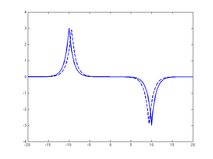
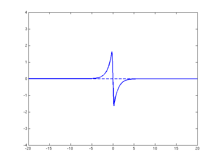
Figure 1. The dashed curve depicts the antisymmetric multipeakon solution $u(t,x)$, which vanishes at $t^{*}$, for $t=0$ (on the left) and $t=t^{*}$ (on the right). The solid curve depicts the multipeakon solution given by $u^{\varepsilon}(t,x)=u(t-\varepsilon,x)$.

Our task is here to identify a metric, which we will denote by $d_{\mathcal{D}}$ for which conservative solutions satisfy a Lipschitz property, that is, if $u$ and $v$ are two solutions of the Camassa–Holm equation, then

$$d_{\mathcal{D}}(u(t),v(t))\leq C_{T}d_{\mathcal{D}}(u_{0},v_{0}),\quad t\in[0,T]$$

for any given, positive $T$. For nonlinear partial differential equations this is in general a quite nontrivial issue. Let us illustrate it in the case of hyperbolic conservation laws

$$u_{t}+f(u)_{x}=0,\quad u|_{t=0}=u_{0}.$$

In the scalar case with $u=u(x,t)\in\mathbb{R}$, $x\in\mathbb{R}$, it is well-known [10] that the solution is $L^{1}$-contractive in the sense that

$$\left\|u(t)-v(t)\right\|_{L^{1}(\mathbb{R})}\leq\left\|u_{0}-v_{0}\right\|_{L^{1}(\mathbb{R})},\quad t\in[0,\infty).$$

In the case of systems, i.e., for $u\in\mathbb{R}^{n}$ with $n>1$ it is known [10] that

$$\left\|u(t)-v(t)\right\|_{L^{1}(\mathbb{R})}\leq C\left\|u_{0}-v_{0}\right\|_{L^{1}(\mathbb{R})},\quad t\in[0,\infty),$$

for some constant $C$. More relevant for the current study, but less well-known, is the recent analysis [5] of the Hunter–Saxton (HS) equation

$$u_{t}+uu_{x}=\frac{1}{4}\Big{(}\int_{-\infty}^{x}u_{x}^{2}\,dx-\int_{x}^{\infty}u_{x}^{2}\,dx\Big{)},\quad u|_{t=0}=u_{0},$$ (1.4)

or alternatively

$$(u_{t}+uu_{x})_{x}=\frac{1}{2}u_{x}^{2},\quad u|_{t=0}=u_{0},$$ (1.5)

which was first introduced in [16] as a model for liquid crystals. Again the equation enjoys wave breaking in finite time and the solutions are not Lipschitz in term of convex norms. The Hunter–Saxton equation can in some sense be considered as a simplified version of the Camassa–Holm equation, and the construction of the semigroup of solutions via a change of coordinates given in [5] is very similar to the one used here and in [14] for the Camassa–Holm equation. In [5] the authors constructed a Riemannian metric which renders the conservative flow generated by the Hunter–Saxton equation Lipschitz continuous on an appropriate function space.

For the Camassa–Holm equation, the problem of continuation beyond wave breaking has been considered by Bressan and Constantin [2, 3] and Holden and Raynaud [12, 14, 15] (see also Xin and Zhang [17, 18] and Coclite, Karlsen, and Holden [8, 9]). Both approaches are based on a reformulation (distinct in the two approaches) of the Camassa–Holm equation as a semilinear system of ordinary differential equations taking values in a Banach space. This formulation allows one to continue the solution beyond collision time, giving either a global conservative solution where the energy is conserved for almost all times or a dissipative solution where energy may vanish from the system. Local existence of the semilinear system is obtained by a contraction argument. Going back to the original function $u$, one obtains a global solution of the Camassa–Holm equation.

In [4], Bressan and Fonte introduce a new distance function $J(u,v)$ which is defined as a solution of an optimal transport problem. They consider two multipeakon solutions $u(t)$ and $v(t)$ of the Camassa–Holm equation and prove, on the intervals of times where no collisions occur, that the growth of $J(u(t),v(t))$ is linear (that is, $\frac{dJ}{dt}(u(t),v(t))\leq CJ(u(t),v(t))$ for some fixed constant $C$) and that $J(u(t),v(t))$ is continuous across collisions. It follows that

$$J(u(t),v(t))\leq e^{CT}J(u(0),v(0))$$ (1.6)

for all times $t$ that are not collision times and, in particular, for almost all times. By density, they construct solutions for any initial data (not just the multipeakons) and the Lipschitz continuity follows from (1.6). As in [4], the goal of this article is to construct a metric which makes the flow Lipschitz continuous. However, we base the construction of the metric directly on the reformulation of the equation which is used to construct the solutions themselves, and we use some fundamental geometrical properties of this reformulation (relabeling invariance, see below). The metric is defined on the set $\mathcal{D}$ which includes configurations where part of the energy is concentrated on sets of measure zero; a natural choice for conservative solutions. In particular, we obtain that the Lipschitz continuity holds for all times and not just for almost all times as in [4].

Let us describe in some detail the approach in this paper, which follows [14] quite closely in setting up the reformulated equation. Let $u=u(t,x)$ denote the solution, and $y(t,\xi)$ the corresponding characteristics, thus $y_{t}(t,\xi)=u(t,y(t,\xi))$. Our new variables are $y(t,\xi)$,

$$U(t,\xi)=u(t,y(t,\xi)),\quad H(t,\xi)=\int_{y(t,0)}^{y(t,\xi)}(u^{2}+u_{x}^{2})\,dx$$ (1.7)

where $U$ corresponds to the Lagrangian velocity while $H$ could be interpreted as the Lagrangian cumulative energy distribution. In the periodic case one defines

$$Q =\frac{1}{2(e-1)}\int_{0}^{1}\sinh(y(\xi)-y(\eta))(U^{2}y_{\xi}+H_{\xi})(\eta)\,d\eta$$ (1.8)

$$\qquad-\frac{1}{4}\int_{0}^{1}\operatorname{sign}(\xi-\eta)\exp\big{(}-\operatorname{sign}(\xi-\eta)(y(\xi)-y(\eta))\big{)}(U^{2}y_{\xi}+H_{\xi})(\eta)\,d\eta,$$

$$P =\frac{1}{2(e-1)}\int_{0}^{1}\cosh(y(\xi)-y(\eta))(U^{2}y_{\xi}+H_{\xi})(\eta)\,d\eta$$ (1.9)

$$\qquad+\frac{1}{4}\int_{0}^{1}\exp\big{(}-\operatorname{sign}(\xi-\eta)(y(\xi)-y(\eta))\big{)}(U^{2}y_{\xi}+H_{\xi})(\eta)\,d\eta.$$

Then one can show that

$$\left\{\begin{aligned} y_{t}&=U,\\ U_{t}&=-Q,\\ H_{t}&=[U^{3}-2PU]_{0}^{\xi},\end{aligned}\right.$$ (1.10)

is equivalent to the Camassa–Holm equation. Global existence of solutions of (1.10) is obtained starting from a contraction argument, see Theorem 2.4. The issue of continuation of the solution past wave breaking is resolved by considering the set $\mathcal{D}$ (see Definition 5.1) which consists of pairs $(u,\mu)$ such that $(u,\mu)\in\mathcal{D}$ if $u\in H^{1}_{\text{\rm per}}$ and $\mu$ is a positive Radon measure with period one, and whose absolutely continuous part satisfies $\mu_{\text{\rm ac}}=(u^{2}+u_{x}^{2})\,dx$. With three Lagrangian variables $(y,U,H)$ versus two Eulerian variables $(u,\mu)$, it is clear that there can be no bijection between the two coordinate systems. If two Lagrangian variables correspond to one and the same solution in Eulerian variables, we say that the Lagrangian variables are relabelings of each other. To resolve the relabeling issue we define a group of transformations which acts on the Lagrangian variables and lets the system of equations (1.10) invariant. We are able to establish a bijection between the space of Eulerian variables and the space of Lagrangian variables when we identify variables that are invariant under the action of the group. This bijection allows us to transform the results obtained in the Lagrangian framework (in which the equation is well-posed) into the Eulerian framework (in which the situation is much more subtle). To obtain a Lipschitz metric in Eulerian coordinates we start by constructing one in the Lagrangian setting. To this end we start by identifying a set $\mathcal{F}$ (see Definition 2.2) that leaves the flow (1.10) invariant, that is, if $X_{0}\in\mathcal{F}$ then the solution $X(t)$ of (1.10) with $X(0)=X_{0}$ will remain in $\mathcal{F}$, i.e., $X(t)\in\mathcal{F}$. Next, we identify a subgroup $G$, see Definition 3.1, of the group of homeomorphisms on the unit interval, and we interpret $G$ as the set of relabeling functions. From this we define a natural group action of $G$ on $\mathcal{F}$, that is, $\Phi(f,X)=X\bullet f$ for $f\in G$ and $X\in\mathcal{F}$, see Definition 3.1 and Proposition 3.3. We can then consider the quotient space ${\mathcal{F}/G}$. However, we still have to identify a unique element in $\mathcal{F}$ for each equivalence class in ${\mathcal{F}/G}$. To this end we introduce the set $\mathcal{H}$, see (3.6), of elements in $\mathcal{F}$ for which $\int_{0}^{1}y(\xi)d\xi=0$ and $y_{\xi}+H_{\xi}=1+\left\|H_{\xi}\right\|_{L^{1}}$. This establishes a bijection between ${\mathcal{F}/G}$ and $\mathcal{H}$, see Lemma 3.5, and therefore between $\mathcal{H}$ and $\mathcal{D}$. Finally, we define a semigroup $\bar{S}_{t}(X_{0})=X(t)$ on $\mathcal{H}$ (Definition 3.7), and the next task is to identify a metric that makes the flow $\bar{S}_{t}$ Lipschitz continuous on $\mathcal{H}$. We use the bijection between $\mathcal{H}$ and $\mathcal{D}$ to transport the metric from $\mathcal{H}$ to $\mathcal{D}$ and get a Lipschitz continuous flow on $\mathcal{D}$.

In [14], the authors define the metric on $\mathcal{H}$ by simply taking the norm of the underlying Banach space (the set $\mathcal{H}$ is a nonlinear subset of a Banach space). They obtain in this way a metric which makes the flow continuous but not Lipschitz continuous. As we will see (see Remark 4.8), this metric is stronger than the one we construct here and for which the flow is Lipschitz continuous. In [5], for the Hunter–Saxton equation, the authors use ideas from Riemannian geometry and construct a semimetric which identifies points that belong to the same equivalence class. The Riemannian framework seems however too rigid for the Camassa–Holm equation, and we have not been able to carry out this approach. However, we retain the essential idea which consists of finding a semimetric which identifies equivalence classes. Instead of a Riemannian metric, we use a discrete counterpart. Note that this technique will also work for the Hunter–Saxton and will give the same metric as in [5]. A natural candidate for a semimetric which identifies equivalence classes is (cf. (4.1))

$$J(X,Y)=\inf_{f,g\in G}\left\|X\bullet f-Y\bullet g\right\|,$$

which is invariant with respect to relabeling. However, it does not satisfy the triangle inequality. Nevertheless it can be modified to satisfy all the requirements for a metric if we instead define, see Definition 4.2, the following quantity

$$d(X,Y)=\inf\sum_{i=1}^{N}J(X_{n-1},X_{n})$$ (1.11)

where the infimum is taken over all finite sequences $\{X_{n}\}_{n=0}^{N}\in\mathcal{F}$ which satisfy $X_{0}=X$ and $X_{N}=Y$. One can then prove that $d(X,Y)$ is a metric on $\mathcal{H}$, see Lemma 4.7. Finally, we prove that the flow is Lipschitz continuous in this metric, see Theorem 4.9. To transfer this result to the Eulerian variables we reconstruct these variables from the Lagrangian coordinates as in [14]: Given $X\in\mathcal{F}$, we define $(u,\mu)\in\mathcal{D}$ by (see Definition 5.3) $u(x)=U(\xi)$ for any $\xi$ such that $x=y(\xi)$, and $\mu=y_{\#}(\nu d\xi)$. We denote the mapping from $\mathcal{F}$ to $\mathcal{D}$ by $M$, and the inverse restricted to $\mathcal{H}$ by $L$. The natural metric on $\mathcal{D}$, denoted $d_{\mathcal{D}}$, is then defined by $d_{\mathcal{D}}((u,\mu),(\tilde{u},\tilde{\mu}))=d(L(u,\mu),L(\tilde{u},\tilde{\mu}))$ for two elements $(u,\mu),(\tilde{u},\tilde{\mu})$ in $\mathcal{D}$, see Definition 5.7. The main theorem, Theorem 5.9, then states that the metric $d_{\mathcal{D}}$ is Lipschitz continuous on all states with finite energy. In the last section, Section 6, the metric is compared with the standard norms. Two results are proved: The mapping $u\mapsto(u,(u^{2}+u_{x}^{2})dx)$ is continuous from $H^{1}_{\rm per}$ into $\mathcal{D}$ (Proposition 6.1). Furthermore, if $(u_{n},\mu_{n})$ is a sequence in $\mathcal{D}$ that converges to $(u,\mu)$ in $\mathcal{D}$. Then $u_{n}\rightarrow u$ in $L^{\infty}_{\rm per}$ and $\mu_{n}\overset{\ast}{\rightharpoonup}\mu$ (Proposition 6.2).

The problem of Lipschitz continuity can nicely be illustrated in the simpler context of ordinary differential equations. Consider three differential equations:

$$\dot{x} =a(x), x(0) =x_{0},\quad\text{$a$ Lipschitz},$$ (1.12a)

$$\dot{x} =1+\alpha H(x), x(0) =x_{0},\quad\text{$H$ the Heaviside function, $\alpha>0$},$$ (1.12b)

$$\dot{x} =\left|x\right|^{1/2}, x(0) =x_{0},\quad\quad\text{$t\mapsto x(t)$ strictly increasing}.$$ (1.12c)

Straightforward computations give as solutions

$$x(t) =x_{0}+\int_{0}^{t}a(x(s))\,ds,$$ (1.13a)

$$x(t) =(1+\alpha H(t-t_{0}))(t-t_{0}),\quad t_{0}=-x_{0}/(1+\alpha H(x_{0})),$$ (1.13b)

$$x(t) =\operatorname{sign}\big{(}\frac{t}{2}+v_{0}\big{)}\big{(}\frac{t}{2}+v_{0}\big{)}^{2}\text{ where }v_{0}=\operatorname{sign}(x_{0})\left|x_{0}\right|^{1/2}.$$ (1.13c)

We find that

$$\left|x(t)-\bar{x}(t)\right| \leq e^{Lt}\left|x_{0}-\bar{x}_{0}\right|,\quad L=\left\|a\right\|_{\rm Lip},$$ (1.14a)

$$\left|x(t)-\bar{x}(t)\right| \leq(1+\alpha)\left|x_{0}-\bar{x}_{0}\right|,$$ (1.14b)

$$x(t)-\bar{x}(t) =t(x_{0}-\bar{x}_{0})^{1/2}+\left|x_{0}-\bar{x}_{0}\right|,\quad\text{when $\bar{x}_{0}=0$, $t>0$, $x_{0}>0$.}$$ (1.14c)

Thus we see that in the regular case (1.12a) we get a Lipschitz estimate with constant $e^{Lt}$ uniformly bounded as $t$ ranges on a bounded interval. In the second case (1.12b) we get a Lipschitz estimate uniformly valid for all $t\in\mathbb{R}$. In the final example (1.12c), by restricting attention to strictly increasing solutions of the ordinary differential equations, we achieve uniqueness and continuous dependence on the initial data, but without any Lipschitz estimate at all near the point $x_{0}=0$. We observe that, by introducing the Riemannian metric

$$d(x,\bar{x})=\left|\int_{x}^{\bar{x}}\frac{dz}{{\left|z\right|^{1/2}}}\right|,$$ (1.15)

an easy computation reveals that

$$d(x(t),\bar{x}(t))=d(x_{0},\bar{x}_{0}).$$ (1.16)

Let us explain why this metric can be considered as a Riemannian metric. The Euclidean metric between the two points is then given

$$\left|x_{0}-\bar{x}_{0}\right|=\inf_{x}\int_{0}^{1}\left|x_{s}(s)\right|\,ds$$ (1.17)

where the infimum is taken over all paths $x\colon[0,1]\to\mathbb{R}$ that join the two points $x_{0}$ and $\bar{x}_{0}$, that is, $x(0)=x_{0}$ and $x(1)=\bar{x}_{0}$. However, as we have seen, the solutions are not Lipschitz for the Euclidean metric. Thus we want to measure the infinitesimal variation $x_{s}$ in an alternative way, which makes solutions of equation (1.12c) Lipschitz continuous. We look at the evolution equation that governs $x_{s}$ and, by differentiating (1.12c) with respect to $s$, we get

$$\dot{x}_{s}=\frac{\operatorname{sign}(x)x_{s}}{2\sqrt{\left|x\right|}},$$

and we can check that

$$\frac{d}{dt}\left(\frac{\left|x_{s}\right|}{\sqrt{\left|x\right|}}\right)=0.$$ (1.18)

Let us consider the real line as a Riemannian manifold where, at any point $x\in\mathbb{R}$, the Riemannian norm is given by $\left|v\right|/\sqrt{\left|x\right|}$ for any tangent vector $v\in\mathbb{R}$ in the tangent space of $x$. From (1.18), one can see that at the infinitesimal level, this Riemannian norm is exactly preserved by the evolution equation. The distance on the real line which is naturally inherited by this Riemannian is given by

$$d(x_{0},\bar{x}_{0})=\inf_{x}\int_{0}^{1}\frac{\left|x_{s}\right|}{\sqrt{\left|x\right|}}\,ds$$

where the infimum is taken over all paths $x\colon[0,1]\to\mathbb{R}$ joining $x_{0}$ and $\bar{x}_{0}$. It is quite reasonable to restrict ourselves to paths that satisfy $x_{s}\geq 0$ and then, by a change of variables, we recover the definition (1.15).

The Riemannian approach to measure a distance between any two distinct points in a given set (as defined in (1.17)) requires the existence of a smooth path between points in the set. In the case of the Hunter–Saxton (see [5]), we could embed the set we were primarily interested in into a convex set (which is therefore connected) and which also could be regularized (so that the Riemannian metric we wanted to use in that case could be defined). In the case of the Camassa–Holm equation, we have been unable to construct such a set. However, there exists the alternative approach which, instead of using a smooth path to join points, uses finite sequences of points, see (1.11). We illustrate this approach with equation (1.12c). We want to define a metric in $(0,\infty)$ which makes the semigroup of solutions Lipschitz stable. Given two points $x,\bar{x}\in(0,\infty)$, we define the function $J\colon(0,\infty)\times(0,\infty)\to[0,\infty)$ as

$$J(x,\bar{x})=\begin{cases}\frac{x-\bar{x}}{\bar{x}^{1/2}}&\text{ if $x\geq\bar{x}$,}\\[5.69054pt] \frac{\bar{x}-x}{x^{1/2}}&\text{ if $x<\bar{x}$}.\end{cases}$$

The function $J$ is symmetric and $J(x,\bar{x})=0$ if and only if $x=\bar{x}$, but $J$ does not satisfy the triangle inequality. Therefore we define (cf. (1.11))

$$d(x,\bar{x})=\inf\sum_{n=0}^{N}J(x_{n},x_{n+1})$$ (1.19)

where the infimum is taken over all finite sequences $\{x_{n}\}_{n=0}^{N}$ such that $x_{0}=x$ and $x_{N}=\bar{x}$. Then, $d$ satisfies the triangle inequality and one can prove that it is also a metric. Given $x_{n},x_{n+1}\in E$ such that $x_{n}\leq x_{n+1}$, we denote $x_{n}(t)$ and $x_{n+1}(t)$ the solution of (1.12c) with initial data $x_{n}$ and $x_{n+1}$, respectively. After a short computation, we get

$$\frac{d}{dt}J(x_{n}(t),x_{n+1}(t))=-\frac{1}{2x_{n}}(x_{n}+x_{n+1}-2\sqrt{x_{n}x_{n+1}})\leq 0.$$

Hence, $J(x_{n}(t),x_{n+1}(t))\leq J(x_{n},x_{n+1})$ so that

$$d(x(t),\bar{x}(t))\leq d(x,\bar{x})$$

and the semigroup of solutions to (1.12c) is a contraction for the metric $d$. It follows from the definition of $J$ that, for $x_{1},x_{2},x_{3}\in E$ with $x_{1}<x_{2}<x_{3}$, we have

$$J(x_{1},x_{2})+J(x_{2},x_{3})<J(x_{1},x_{3}).$$ (1.20)

It implies that $d(x,\bar{x})$ satisfies

$$d(x,\bar{x})=\inf_{\delta}\sum_{n=0}^{N}J(x_{n},x_{n+1})$$

where $\delta=\min_{n}\left|x_{n+1}-x_{n}\right|$, which is also the definition of the Riemann integral, so that

$$d(x,\bar{x})=\int_{x}^{\bar{x}}\frac{1}{\sqrt{z}}\,dz$$

and the metric we have just defined coincides with the Riemannian metric we have introduced. Note that if we choose

$$\bar{J}(x,\bar{x})=\begin{cases}\frac{x-\bar{x}}{x^{1/2}}&\text{ if $x\geq\bar{x}$}\\ \frac{\bar{x}-x}{\bar{x}^{1/2}}&\text{ if $x<\bar{x}$},\end{cases}$$

then (1.20) does not hold; we have instead $\bar{J}(x_{1},x_{3})<\bar{J}(x_{1},x_{2})+\bar{J}(x_{2},x_{3})$, which is the triangle inequality. Thus, for $\bar{d}$ as defined by (1.19) with $J$ replaced by $\bar{J}$, we get

$$\bar{d}(x,\bar{x})=\bar{J}(x,\bar{x})\neq\int_{x}^{\bar{x}}\frac{1}{\sqrt{z}}\,dz.$$

It is also possible to check that, for $\bar{J}$, we cannot get that $\bar{J}(x_{n}(t),x_{n+1}(t))\leq C\bar{J}(x_{n},x_{n+1})$ for any constant $C$ for any $x_{n}$ and $x_{n+1}$ and $t\in[0,T]$ (for a given $T$), so that the definition of $\bar{J}$ is inappropriate to obtain results of stability for (1.12c).

2. Semi-group of solutions in Lagrangian coordinates

The Camassa–Holm equation for $\kappa=0$ reads

$$u_{t}-u_{xxt}+3uu_{x}-2u_{x}u_{xx}-uu_{xxx}=0,$$ (2.1)

and can be rewritten as the following system

$$u_{t}+uu_{x}+P_{x} =0,$$ (2.2)

$$P-P_{xx} =u^{2}+\frac{1}{2}u_{x}^{2}.$$ (2.3)

We consider periodic solutions of period one. Next, we rewrite the equation in Lagrangian coordinates. Therefore we introduce the characteristics

$$y_{t}(t,\xi)=u(t,y(t,\xi)).$$ (2.4)

We introduce the space $V_{1}$ defined as

$$V_{1}=\{f\in{W^{1,1}_{\text{\rm loc}}}(\mathbb{R})\mid f(\xi+1)=f(\xi)+1\,\text{for all }\xi\in\mathbb{R}\}.$$

Functions in $V_{1}$ map the unit interval into itself in the sense that if $u$ is periodic with period 1, then $u\circ f$ is also periodic with period 1. The Lagrangian velocity $U$ reads

$$U(t,\xi)=u(t,y(t,\xi)).$$ (2.5)

We will consider $y\in V_{1}$ and $U$ periodic. We define the Lagrangian energy cumulative distribution as

$$H(t,\xi)=\int_{y(t,0)}^{y(t,\xi)}(u^{2}+u_{x}^{2})(t,x)\,dx.$$ (2.6)

For all $t$, the function $H$ belongs to the vector space $V$ defined as follows:

$$V=\{f\in{W^{1,1}_{\text{\rm loc}}}(\mathbb{R})\mid\text{there exists $\alpha\in\mathbb{R}$}\\ \text{such that $f(\xi+1)=f(\xi)+\alpha$ for all $\xi\in\mathbb{R}$}\}.$$

Equip $V$ with the norm

$$\left\|f\right\|_{V}=\left\|f\right\|_{L^{\infty}([0,1])}+\left\|f_{\xi}\right\|_{L^{1}([0,1])}.$$

As an immediate consequence of the definition of the characteristics we obtain

$$U_{t}(t,\xi)=u_{t}(t,y)+y_{t}(t,\xi)u_{x}(t,y)=-P_{x}\circ y(t,\xi).$$ (2.7)

This last term can be expressed uniquely in term of $U$, $y$, and $H$. We have the following explicit expression for $P$,

$$P(t,x)=\frac{1}{2}\int_{\mathbb{R}}e^{-\left|x-z\right|}(u^{2}(t,z)+\frac{1}{2}u_{x}^{2}(t,z))\,dz.$$ (2.8)

Thus,

$$P_{x}\circ{y}(t,\xi)=-\frac{1}{2}\int_{\mathbb{R}}\operatorname{sign}(y(t,\xi)-z)e^{-\left|y(t,\xi)-z\right|}(u^{2}(t,z)+\frac{1}{2}u_{x}^{2}(t,z))\,dz,$$

and, after the change of variables $z=y(t,\eta)$,

$$P_{x}\circ y(t,\xi)=-\frac{1}{2}\int_{\mathbb{R}}\Big{[}\operatorname{sign}(y(t,\xi)-y(t,\eta))e^{-\left|y(t,\xi)-y(t,\eta)\right|}\\ \times\left(u^{2}(t,y(t,\eta))+\frac{1}{2}u_{x}^{2}(t,y(t,\eta))\right)y_{\xi}(t,\eta)\Big{]}\,d\eta.$$ (2.9)

We have

$$H_{\xi}=(u^{2}+u_{x}^{2})\circ{y}y_{\xi}=:\nu.$$ (2.10)

Note that $\nu$ is periodic with period one. Then, (2.9) can be rewritten as

$$P_{x}\circ{y}(\xi)=-\frac{1}{4}\int_{\mathbb{R}}\operatorname{sign}(y(\xi)-y(\eta))\exp(-\left|y(\xi)-y(\eta)\right|)\big{(}U^{2}y_{\xi}+\nu\big{)}(\eta)\,d\eta,$$ (2.11)

where the $t$ variable has been dropped to simplify the notation. Later we will prove that $y$ is an increasing function for any fixed time $t$. If, for the moment, we take this for granted, then $P_{x}\circ{y}$ is equivalent to $Q$ where

$$Q(t,\xi)=-\frac{1}{4}\int_{\mathbb{R}}\operatorname{sign}(\xi-\eta)\exp\big{(}-\operatorname{sign}(\xi-\eta)(y(\xi)-y(\eta))\big{)}\big{(}U^{2}y_{\xi}+\nu\big{)}(\eta)\,d\eta,$$ (2.12)

and, slightly abusing the notation, we write

$$P(t,\xi)=\frac{1}{4}\int_{\mathbb{R}}\exp\big{(}-\operatorname{sign}(\xi-\eta)(y(\xi)-y(\eta))\big{)}\big{(}U^{2}y_{\xi}+\nu\big{)}(\eta)\,d\eta.$$ (2.13)

The derivatives of $Q$ and $P$ are given by

$$Q_{\xi}=-\frac{1}{2}\nu-\left(\frac{1}{2}U^{2}-P\right)y_{\xi}\ \text{ and }\ P_{\xi}=Qy_{\xi},$$ (2.14)

respectively. For $\xi\in[0,1]$, using the fact that $y(\xi+1)=y(\xi)+1$ and the periodicity of $\nu$ and $U$, the expressions for $Q$ and $P$ can be rewritten as

$$Q=\frac{1}{2(e-1)}\int_{0}^{1}\sinh(y(\xi)-y(\eta))(U^{2}y_{\xi}+\nu)(\eta)\,d\eta\\ -\frac{1}{4}\int_{0}^{1}\operatorname{sign}(\xi-\eta)\exp\big{(}-\operatorname{sign}(\xi-\eta)(y(\xi)-y(\eta))\big{)}(U^{2}y_{\xi}+\nu)(\eta)\,d\eta,$$ (2.15)

and

$$P=\frac{1}{2(e-1)}\int_{0}^{1}\cosh(y(\xi)-y(\eta))(U^{2}y_{\xi}+\nu)(\eta)\,d\eta\\ +\frac{1}{4}\int_{0}^{1}\exp\big{(}-\operatorname{sign}(\xi-\eta)(y(\xi)-y(\eta))\big{)}(U^{2}y_{\xi}+\nu)(\eta)\,d\eta.$$ (2.16)

Thus $P_{x}\circ y$ and $P\circ y$ can be replaced by equivalent expressions given by (2.12) and (2.13) which only depend on our new variables $U$, $H$, and $y$. We obtain a new system of equations, which is at least formally equivalent to the Camassa–Holm equation:

$$\left\{\begin{aligned} y_{t}&=U,\\ U_{t}&=-Q,\\ H_{t}&=[U^{3}-2PU]_{0}^{\xi}.\end{aligned}\right.$$ (2.17)

After differentiating (2.17) we find

$$\left\{\begin{aligned} y_{\xi t}&=U_{\xi},\\ U_{\xi t}&=\frac{1}{2}\nu+\left(\frac{1}{2}U^{2}-P\right)y_{\xi},\\ H_{\xi t}&=-2Q\,Uy_{\xi}+\left(3U^{2}-2P\right)U_{\xi}.\end{aligned}\right.$$ (2.18)

From (2.17) and (2.18), we obtain the system

$$\left\{\begin{aligned} y_{t}&=U,\\ U_{t}&=-Q,\\ \nu_{t}&=-2Q\,Uy_{\xi}+\left(3U^{2}-2P\right)U_{\xi}.\end{aligned}\right.$$ (2.19)

We can write (2.19) more compactly as

$$X_{t}=F(X),\quad X=(y,U,\nu).$$ (2.20)

Let

$${W^{1,1}_{\text{\rm per}}}=\{f\in{W^{1,1}_{\text{\rm loc}}}(\mathbb{R})\mid f(\xi+1)=f(\xi)\text{ for all }\xi\in\mathbb{R}\}.$$

We equip ${W^{1,1}_{\text{\rm per}}}$ with the norm of $V$, that is,

$$\left\|f\right\|_{{W^{1,1}_{\text{\rm per}}}}=\left\|f\right\|_{L^{\infty}([0,1])}+\left\|f_{\xi}\right\|_{L^{1}([0,1])},$$

which is equivalent to the standard norm of ${W^{1,1}_{\text{\rm per}}}$ because $\left\|f\right\|_{L^{1}([0,1])}\leq\left\|f\right\|_{L^{\infty}([0,1])}\leq\left\|f\right\|_{L^{1}([0,1])}+\left\|f_{\xi}\right\|_{L^{1}([0,1])}$. Let $E$ be the Banach space defined as

$$E=V\times{W^{1,1}_{\text{\rm per}}}\times L^{1}_{\rm per}.$$

We derive the following Lipschitz estimates for $P$ and $Q$.

Lemma 2.1.

For any $X=(y,U,\nu)$ in $E$, we define the maps $\mathcal{Q}$ and $\mathcal{P}$ as $\mathcal{Q}(X)=Q$ and $\mathcal{P}(X)=P$ where $Q$ and $P$ are given by (2.12) and (2.13), respectively. Then, $\mathcal{P}$ and $\mathcal{Q}$ are Lipschitz maps on bounded sets from $E$ to ${W^{1,1}_{\text{\rm per}}}$. More precisely, we have the following bounds. Let

$$B_{M}=\{X=(y,U,\nu)\in E\mid\left\|U\right\|_{{W^{1,1}_{\text{\rm per}}}}+\left\|y_{\xi}\right\|_{L^{1}}+\left\|\nu\right\|_{L^{1}}\leq M\}.$$ (2.21)

Then for any $X,\tilde{X}\in B_{M}$, we have

$$\left\|\mathcal{Q}(X)-\mathcal{Q}(\tilde{X})\right\|_{{W^{1,1}_{\text{\rm per}}}}\leq C_{M}\left\|X-\tilde{X}\right\|_{E}$$ (2.22)

and

$$\left\|\mathcal{P}(X)-\mathcal{P}(\tilde{X})\right\|_{{W^{1,1}_{\text{\rm per}}}}\leq C_{M}\left\|X-\tilde{X}\right\|_{E}$$ (2.23)

where the constant $C_{M}$ only depends on the value of $M$.

Proof.

Let us first prove that $\mathcal{P}$ and $\mathcal{Q}$ are Lipschitz maps from $B_{M}$ to ${L^{\infty}_{\text{\rm per}}}$. Note that by using a change of variables in (2.15) and (2.16), we obtain that $\mathcal{P}$ and $\mathcal{Q}$ are periodic with period $1$. Let now $X=(y,U,\nu)$ and $\tilde{X}=(\tilde{y},\tilde{U},\tilde{\nu})$ be two elements of $B_{M}$. Since the map $x\mapsto\cosh x$ is locally Lipschitz, it is Lipschitz on $[-M,M]$. We denote by $C_{M}$ a generic constant that only depends on $M$. Since, for all $\xi,\eta$ in $[0,1]$ we have $\left|y(\xi)-y(\eta)\right|\leq\left\|y_{\xi}\right\|_{L^{1}}$, we also have

$$\left|\cosh(y(\xi)-y(\eta))-\cosh(\tilde{y}(\xi)-\tilde{y}(\eta))\right| \leq C_{M}\left|y(\xi)-\tilde{y}(\xi)-y(\eta)+\tilde{y}(\eta)\right|$$

$$\leq C_{M}\left\|y-\tilde{y}\right\|_{L^{\infty}}.$$

It follows that, for all $\xi\in[0,1]$,

$$\left\|\cosh(y(\xi)-y(\,\cdot\,))(U^{2}y_{\xi}+\nu)(\,\cdot\,)-\cosh(\tilde{y}(\xi)-\tilde{y}(\,\cdot\,))(\tilde{U}^{2}\tilde{y}_{\xi}+\tilde{\nu})(\,\cdot\,)\right\|_{L^{1}}\\ \leq C_{M}\big{(}\left\|y-\tilde{y}\right\|_{L^{\infty}}+\left\|U-\tilde{U}\right\|_{L^{\infty}}+\left\|y_{\xi}-\tilde{y}_{\xi}\right\|_{L^{1}}+\left\|\nu-\tilde{\nu}\right\|_{L^{1}}\big{)}$$

and the map $X=(y,U,\nu)\mapsto\frac{1}{2(e-1)}\int_{0}^{1}\cosh(y(\xi)-y(\eta))(U^{2}y_{\xi}+\nu)(\eta)\,d\eta$ which corresponds to the first term in (2.16) is Lipschitz from $B_{M}$ to ${L^{\infty}_{\text{\rm per}}}$ and the Lipschitz constant only depends on $M$. We handle the other terms in (2.16) in the same way and we prove that $\mathcal{P}$ is Lipschitz from $B_{M}$ to ${L^{\infty}_{\text{\rm per}}}$. Similarly, one proves that $\mathcal{Q}\colon B_{M}\to{L^{\infty}_{\text{\rm per}}}$ is Lipschitz for a Lipschitz constant which only depends on $M$. Direct differentiation gives the expressions (2.14) for the derivatives $P_{\xi}$ and $Q_{\xi}$ of $P$ and $Q$. Then, as $\mathcal{P}$ and $\mathcal{Q}$ are Lipschitz from $B_{M}$ to ${L^{\infty}_{\text{\rm per}}}$, we have

$$\big{\|} \mathcal{Q}(X)_{\xi}-\mathcal{Q}(\tilde{X})_{\xi}\big{\|}_{L^{1}}$$

$$=\left\|y_{\xi}\mathcal{P}(X)-\tilde{y}_{\xi}\mathcal{P}(\tilde{X})-\frac{1}{2}(U^{2}y_{\xi}-\tilde{U}^{2}\tilde{y}_{\xi})-\nu+\tilde{\nu}\right\|_{L^{1}}$$

$$\leq C_{M}\big{(}\left\|\mathcal{P}(X)-\mathcal{P}(\tilde{X})\right\|_{L^{\infty}}+\left\|U-\tilde{U}\right\|_{L^{\infty}}+\left\|y_{\xi}-\tilde{y}_{\xi}\right\|_{L^{1}}+\left\|\nu-\tilde{\nu}\right\|_{L^{1}}\big{)}$$

$$\leq C_{M}\left\|X-\tilde{X}\right\|_{E}.$$

Hence, we have proved that $\mathcal{Q}\colon B_{M}\to{W^{1,1}_{\text{\rm per}}}$ is Lipschitz for a Lipschitz constant that only depends on $M$. We prove the corresponding result for $\mathcal{P}$ in the same way. ∎

The short-time existence follows from Lemma 2.1 and a contraction argument. Global existence is obtained only for initial data which belong to the set $\mathcal{F}$ as defined below.

Definition 2.2.

The set $\mathcal{F}$ is composed of all $(y,U,\nu)\in E$ such that

$$y\in V_{1},\ (y,U)\in W^{1,\infty}_{\rm loc}(\mathbb{R})\times W^{1,\infty}_{\rm loc}(\mathbb{R}),\ \nu\in L^{\infty},$$ (2.24a)

$$y_{\xi}\geq 0,\ \nu\geq 0,\ y_{\xi}+\nu\geq c\text{ almost everywhere, for some constant $c>0$},$$ (2.24b)

$$y_{\xi}\nu=y_{\xi}^{2}U^{2}+U_{\xi}^{2}\text{ almost everywhere}.$$ (2.24c)

Lemma 2.3.

The set $\mathcal{F}$ is preserved by the equation (2.19), that is, if $X(t)$ solves (2.19) for $t\in[0,T]$ with initial data $X_{0}\in\mathcal{F}$, then $X(t)\in\mathcal{F}$ for all $t\in[0,T]$.

The proof is basically the same as in [14].

Theorem 2.4.

For any $\bar{X}=(\bar{y},\bar{U},\bar{\nu})\in\mathcal{F}$, the system (2.19) admits a unique global solution $X(t)=(y(t),U(t),\nu(t))$ in $C^{1}(\mathbb{R}_{+},E)$ with initial data $\bar{X}=(\bar{y},\bar{U},\bar{\nu})$. We have $X(t)\in\mathcal{F}$ for all times. Let the mapping $S\colon\mathcal{F}\times\mathbb{R}_{+}\to\mathcal{F}$ be defined as

$$S_{t}(X)=X(t).$$

Given $M>0$ and $T>0$, we define $B_{M}$ as before, that is,

$$B_{M}=\{X=(y,U,\nu)\in E\mid\left\|U\right\|_{{W^{1,1}_{\text{\rm per}}}}+\left\|y_{\xi}\right\|_{L^{1}}+\left\|\nu\right\|_{L^{1}}\leq M\}.$$ (2.25)

Then there exists a constant $C_{M}$ which depends only on $M$ and $T$ such that, for any two elements $X_{\alpha}$ and $X_{\beta}$ in $B_{M}$, we have

$$\left\|S_{t}X_{\alpha}-S_{t}X_{\beta}\right\|_{E}\leq C_{M}\left\|X_{\alpha}-X_{\beta}\right\|_{E}$$ (2.26)

for any $t\in[0,T]$.

Proof.

By using Lemma 2.1, we proceed using a contraction argument and obtain the existence of short time solutions to (2.19). Let $T$ by the maximal time of existence and assume $T<\infty$. Let $(y,U,\nu)$ be a solution of (2.19) in $C^{1}([0,T),E)$ with initial data $(y_{0},U_{0},\nu_{0})$. We want to prove that

$$\sup_{t\in[0,T)}\left\|(y(t,\,\cdot\,),U(t,\,\cdot\,),\nu(t,\,\cdot\,))\right\|_{E}<\infty.$$ (2.27)

From (2.19), we get

$$\int_{0}^{1}\nu(t,\xi)\,d\xi =\int_{0}^{1}\nu(0,\xi)\,d\xi+\int_{0}^{1}\int_{0}^{t}(-2Q\,Uy_{\xi}+\left(3U^{2}-2P\right)U_{\xi})(t,\xi)\,dtd\xi$$

$$=\int_{0}^{1}\nu(0,\xi)\,d\xi+\int_{0}^{t}\int_{0}^{1}(U^{3}-2PU)_{\xi}(t,\xi)\,d\xi dt$$

$$=\int_{0}^{1}\nu(0,\xi)\,d\xi.$$ (2.28)

Hence, $\left\|\nu(t,\,\cdot\,)\right\|_{L^{1}}=\left\|\nu(0,\,\cdot\,)\right\|_{L^{1}}$. This identity corresponds to the conservation of the total energy. We now consider a fixed time $t\in[0,T)$ which we omit in the notation when there is no ambiguity. For $\xi$ and $\eta$ in $[0,1]$, we have $\left|y(\xi)-y(\eta)\right|\leq 1$ because $y$ is increasing and $y(1)-y(0)=1$. From (2.24c), we infer $U^{2}y_{\xi}\leq\nu$ and, from (2.15), we obtain

$$\left|Q\right|\leq\frac{1}{e-1}\int_{0}^{1}\sinh(|y(\xi)-y(\eta)|)\nu(\eta)\,d\eta+\int_{0}^{1}e^{-\left|y(\xi)-y(\eta)\right|}\nu(\eta)\,d\eta.$$

Hence,

$$\left\|Q(t,\,\cdot\,)\right\|_{L^{\infty}}\leq C\left\|\nu(t,\,\cdot\,)\right\|_{L^{1}}=C\left\|\nu(0,\,\cdot\,)\right\|_{L^{1}}$$ (2.29)

for some constant $C$. Similarly, one prove that $\left\|P(t,\,\cdot\,)\right\|_{L^{\infty}}\leq C\left\|\nu(0,\,\cdot\,)\right\|_{L^{1}}$ and therefore $\sup_{t\in[0,T)}\left\|Q(t,\,\cdot\,)\right\|_{L^{\infty}}$ and $\sup_{t\in[0,T)}\left\|P(t,\,\cdot\,)\right\|_{L^{\infty}}$ are finite. Since $U_{t}=-Q$, it follows that

$$\left\|U(t,\,\cdot\,)\right\|_{L^{\infty}}\leq\left\|U(0,\,\cdot\,)\right\|_{L^{\infty}}+CT\left\|\nu(0,\,\cdot\,)\right\|_{L^{1}}$$ (2.30)

and $\sup_{t\in[0,T)}\left\|U(t,\,\cdot\,)\right\|_{L^{\infty}}<\infty$. Since $y_{t}=U$, we have that $\sup_{t\in[0,T)}\left\|y(t,\,\cdot\,)\right\|_{L^{\infty}}$ is also finite. Thus, we have proved that

$$C_{1}=\sup_{t\in[0,T)}\{\left\|U(t,\,\cdot\,)\right\|_{L^{\infty}}+\left\|P(t,\,\cdot\,)\right\|_{L^{\infty}}+\left\|Q(t,\,\cdot\,)\right\|_{L^{\infty}}\}$$

is finite and depends only on $T$ and $\left\|U(0,\,\cdot\,)\right\|_{L^{\infty}}+\left\|\nu(0,\,\cdot\,)\right\|_{L^{1}}$. Let $Z(t)=\left\|y_{\xi}(t,\,\cdot\,)\right\|_{L^{1}}+\left\|U_{\xi}(t,\,\cdot\,)\right\|_{L^{1}}+\left\|\nu(t,\,\cdot\,)\right\|_{L^{1}}$. Using the semi-linearity of (2.18) with respect to $(y_{\xi},U_{\xi},\nu)$, we obtain

$$Z(t)\leq Z(0)+C\int_{0}^{t}Z(\tau)\,d\tau$$

where $C$ is a constant depending only on $C_{1}$. It follows from Gronwall’s lemma that $\sup_{t\in[0,T)}Z(t)$ is finite, and this concludes the proof of the global existence.

Moreover we have proved that

$$\left\|U(t,\,\cdot\,)\right\|_{{W^{1,1}_{\text{\rm per}}}}+\left\|y_{\xi}(t,\,\cdot\,)\right\|_{L^{1}}+\left\|\nu(t,\,\cdot\,)\right\|_{L^{1}}\leq C_{M}$$ (2.31)

for a constant $C_{M}$ which depends only on $T$ and $\left\|U(0,\,\cdot\,)\right\|_{{W^{1,1}_{\text{\rm per}}}}+\left\|y_{\xi}(0,\,\cdot\,)\right\|_{L^{1}}+\left\|\nu(0,\,\cdot\,)\right\|_{L^{1}}$. Let us prove (2.26). Given $T$ and $X_{\alpha},X_{\beta}\in B_{M}$, from Lemma 2.1 and (2.31), we get that

$$\left\|U_{\alpha}(t,\,\cdot\,)-U_{\beta}(t,\,\cdot\,)\right\|_{L^{\infty}}+\left\|Q_{\alpha}(t,\,\cdot\,)-Q_{\beta}(t,\,\cdot\,)\right\|_{L^{\infty}}\leq C_{M}\left\|X_{\alpha}(t)-X_{\beta}(t)\right\|_{E}$$

where $C_{M}$ is a generic constant which depends only on $M$ and $T$. Using again (2.18) and Lemma 2.1, we get that for a given time $t\in[0,T]$,

$$\left\|U_{\alpha\xi}-U_{\beta\xi}\right\|_{L^{1}}+\left\|\frac{1}{2}\nu_{\alpha}+\left(\frac{1}{2}U_{\alpha}^{2}-P_{\alpha}\right)y_{\alpha\xi}-\frac{1}{2}\nu_{\beta}-\left(\frac{1}{2}U_{\beta}^{2}-P_{\beta}\right)y_{\beta\xi}\right\|_{L^{1}}\\ +\left\|-2Q_{\alpha}\,U_{\alpha}y_{\alpha\xi}+\left(3U_{\alpha}^{2}-2P_{\alpha}\right)U_{\alpha\xi}+2Q_{\beta}\,U_{\beta}y_{\beta\xi}-\left(3U_{\beta}^{2}-2P_{\beta}\right)U_{\beta\xi}\right\|_{L^{1}}\\ \leq C_{M}\left\|X_{\alpha}-X_{\beta}\right\|_{E}.$$

Hence, $\left\|F(X_{\alpha}(t))-F(X_{\beta}(t))\right\|_{E}\leq C_{M}\left\|X_{\alpha}(t)-X_{\beta}(t)\right\|_{E}$ where $F$ is defined as in (2.20). Then, (2.26) follows from Gronwall’s lemma applied to (2.20). ∎

3. Relabeling invariance

We denote by $G$ the subgroup of the group of homeomorphisms on the unit interval defined as follows:

Definition 3.1.

Let $G$ be the set of all functions $f$ such that $f$ is invertible,

$$f\in W_{\rm loc}^{1,\infty}(\mathbb{R}),\ f(\xi+1)=f(\xi)+1\text{ for all }\xi\in\mathbb{R}\text{, and }$$ (3.1)

$$f-\operatorname{id}\text{ and }f^{-1}-\operatorname{id}\text{ both belong to }{W^{1,\infty}_{\text{\rm per}}}.$$ (3.2)

The set $G$ can be interpreted as the set of relabeling functions. Note that $f\in G$ implies that

$$\frac{1}{1+\alpha}\leq f_{\xi}\leq 1+\alpha$$

for some constant $\alpha>0$. This condition is also almost sufficient as Lemma 3.2 in [14] shows. Given a triplet $(y,U,\nu)\in\mathcal{F}$, we denote by $h$ the total energy $\left\|\nu\right\|_{L^{1}}$. We define the subsets $\mathcal{F}_{\alpha}$ of $\mathcal{F}$ as follows

$$\mathcal{F}_{\alpha}=\{X=(y,U,\nu)\in\mathcal{F}\mid\frac{1}{1+\alpha}\leq\frac{1}{1+h}(y_{\xi}+\nu)\leq 1+\alpha\}.$$

The set $\mathcal{F}_{0}$ is then given by

$$\mathcal{F}_{0}=\{X=(y,U,\nu)\in\mathcal{F}\mid y_{\xi}+\nu=1+h\}.$$ (3.3)

We have $\mathcal{F}=\cup_{\alpha\geq 0}\mathcal{F}_{\alpha}$. We define the action of the group $G$ on $\mathcal{F}$.

Definition 3.2.

We define the map $\Phi\colon G\times\mathcal{F}\to\mathcal{F}$ as follows

$$\left\{\begin{aligned} \bar{y}&=y\circ f,\\ \bar{U}&=U\circ f,\\ \bar{\nu}&=\nu\circ ff_{\xi},\end{aligned}\right.$$

where $(\bar{y},\bar{U},\bar{\nu})=\Phi(f,(y,U,\nu))$. We denote $(\bar{y},\bar{U},\bar{\nu})=(y,U,\nu)\bullet f$.

Proposition 3.3.

The map $\Phi$ defines a group action of $G$ on $\mathcal{F}$.

Proof.

By the definition it is clear that $\Phi$ satisfies the fundamental property of a group action, that is $X\bullet f_{1}\bullet f_{2}=X\bullet(f_{1}\circ f_{2})$ for all $X\in\mathcal{F}$ and $f_{1}$, $f_{2}\in G$. It remains to prove that $X\bullet f$ indeed belongs to $\mathcal{F}$. We denote $\hat{X}=(\hat{y},\hat{U},\hat{\nu})=X\bullet f$, then it is not hard to check that $\hat{y}(\xi+1)=\hat{y}(\xi)+1$, $\hat{U}(\xi+1)=\hat{U}(\xi)$, and $\hat{\nu}(\xi+1)=\hat{\nu}(\xi)$ for all $\xi\in\mathbb{R}$. By definition we have $\hat{v}=v\circ ff_{\xi}$, and we will now prove that

$$\hat{y}_{\xi}=y_{\xi}\circ ff_{\xi},\quad\text{ and }\quad\hat{U}_{\xi}=U_{\xi}\circ ff_{\xi},$$

almost everywhere. Let $B_{1}$ be the set where $y$ is differentiable and $B_{2}$ the set where $\hat{y}$ and $f$ are differentiable. Using Rademacher’s theorem, we get that $\operatorname{meas}(B_{1}^{c})=\operatorname{meas}(B_{2}^{c})=0$. For $\xi\in B_{3}=B_{2}\cap f^{-1}(B_{1})$, we consider a sequence $\xi_{i}$ converging to $\xi$ with $\xi_{i}\not=\xi$ for all $i\in\mathbb{N}$. We have

$$\frac{y(f(\xi_{i}))-y(f(\xi))}{f(\xi_{i})-f(\xi)}\frac{f(\xi_{i})-f(\xi)}{\xi_{i}-\xi}=\frac{\hat{y}(\xi_{i})-\hat{y}(\xi)}{\xi_{i}-\xi}.$$ (3.4)

Since $f$ is continuous, $f(\xi_{i})$ converges to $f(\xi)$ and, as $y$ is differentiable at $f(\xi)$, the left-hand side of (3.4) tends to $y_{\xi}\circ f(\xi)f_{\xi}(\xi)$, the right-hand side of (3.4) tends to $\hat{y}_{\xi}(\xi)$, and we get

$$y_{\xi}(f(\xi))f_{\xi}(\xi)=\hat{y}_{\xi}(\xi),$$ (3.5)

for all $\xi\in B_{3}$. Since $f^{-1}$ is Lipschitz continuous, one-to-one, and $\operatorname{meas}(B_{1}^{c})=0$, we have $\operatorname{meas}(f^{-1}(B_{1})^{c})=0$ and therefore (3.5) holds almost everywhere. One proves the other identity similarly. As $f_{\xi}>0$ almost everywhere, we obtain immediately that (2.24b) and (2.24c) are fulfilled. That (2.24a) is also satisfied follows from the following considerations: $\left\|\hat{y}_{\xi}\right\|_{L^{1}}=\left\|y_{\xi}\right\|_{L^{1}}$, as $y_{\xi}$ is periodic with period $1$. The same argument applies when considering $\left\|\hat{U}_{\xi}\right\|_{L^{1}}$ and $\left\|\hat{\nu}\right\|_{L^{1}}$. As $U$ is periodic with period $1$, we can also conclude that $\left\|\hat{U}\right\|_{L^{\infty}}=\left\|U\right\|_{L^{\infty}}$. As $f\in G$, one obtains that $\left\|\hat{y}\right\|_{L^{\infty}}$ is bounded, but not equal to $\left\|y\right\|_{L^{\infty}}$. ∎

Note that the set $B_{M}$ is invariant with respect to relabeling while the $E$-norm is not, as the following example shows: Consider the function $y(\xi)=\xi\in V_{1}$, and $f\in G$, then this yields

$$\left\|y(f(\xi))\right\|_{L^{\infty}([0,1])}=\left\|f(\xi)\right\|_{L^{\infty}([0,1])}.$$

Hence, the $L^{\infty}$-norm of $y(f(\xi))$ will always depend on $f$.

Since $G$ is acting on $\mathcal{F}$, we can consider the quotient space ${\mathcal{F}/G}$ of $\mathcal{F}$ with respect to the group action. Let us introduce the subset $\mathcal{H}$ of $\mathcal{F}_{0}$ defined as follows

$$\mathcal{H}=\{(y,U,\nu)\in\mathcal{F}_{0}\mid\int_{0}^{1}y(\xi)\,d\xi=0\}.$$ (3.6)

It turns out that $\mathcal{H}$ contains a unique representative in $\mathcal{F}$ for each element of ${\mathcal{F}/G}$, that is, there exists a bijection between $\mathcal{H}$ and ${\mathcal{F}/G}$. In order to prove this we introduce two maps $\Pi_{1}\colon\mathcal{F}\to\mathcal{F}_{0}$ and $\Pi_{2}\colon\mathcal{F}_{0}\to\mathcal{H}$ defined as follows

$$\Pi_{1}(X)=X\bullet f^{-1}$$ (3.7)

with $f=\frac{1}{1+h}(y+\int_{0}^{\xi}\nu(\eta)\,d\eta)\in G$ and $X=(y,U,\nu)$, and

$$\Pi_{2}(X)=X(\xi-a)$$ (3.8)

with $a=\int_{0}^{1}y(\xi)\,d\xi$. First, we have to prove that $f$ indeed belongs to $G$. We have

$$f(\xi+1) =\frac{1}{1+h}\big{(}y(\xi+1)+\int_{0}^{\xi+1}\nu(\eta)\,d\eta\big{)}$$

$$=\frac{1}{1+h}\big{(}y(\xi)+1+\int_{0}^{\xi}\nu(\eta)\,d\eta+h\big{)}=f(\xi)+1$$

and this proves (3.1). Since $(y,U,\nu)\in\mathcal{F}$, there exists a constant $c\geq 1$ such that $\frac{1}{c}\leq f_{\xi}\leq c$ for almost every $\xi$ and therefore (3.2) follows from an application of Lemma 3.2 in [14]. After noting that the group action lets the quantity $h=\left\|\nu\right\|_{L^{1}}$ invariant, it is not hard to check that $\Pi_{1}(X)$ indeed belongs to $\mathcal{F}_{0}$, that is, $\frac{1}{1+\bar{h}}(\bar{y}_{\xi}+\bar{\nu})=1$ where we denote $(\bar{y},\bar{U},\bar{\nu})=\Pi_{1}(X)$. Let us prove that $(\bar{y},\bar{U},\bar{\nu})=\Pi_{2}(y,U,\nu)$ belongs to $\mathcal{H}$ for any $(y,U,\nu)\in\mathcal{F}_{0}$. On the one hand, we have $\frac{1}{1+\bar{h}}(\bar{y}_{\xi}+\bar{\nu})=1$ because $\bar{h}=h$ and $\frac{1}{1+h}(y_{\xi}+\nu)=1$ as $(y,U,\nu)\in\mathcal{F}_{0}$. On the other hand,

$$\int_{0}^{1}\bar{y}(\xi)\,d\xi=\int_{-a}^{1-a}y(\xi)\,d\xi=\int_{0}^{1}y(\xi)\,d\xi+\int_{-a}^{0}y(\xi)\,d\xi+\int_{1}^{1-a}y(\xi)\,d\xi$$ (3.9)

and, since $y(\xi+1)=y(\xi)+1$, we obtain

$$\int_{0}^{1}\bar{y}(\xi)\,d\xi=\int_{0}^{1}y(\xi)\,d\xi+\int_{-a}^{0}y(\xi)\,d\xi+\int_{0}^{-a}y(\xi)\,d\xi-a=\int_{0}^{1}y(\xi)\,dx-a=0.$$ (3.10)

Thus $\Pi_{2}(X)\in\mathcal{H}$. Note that the definition (3.8) of $\Pi_{2}$ can be rewritten as

$$\Pi_{2}(X)=X\bullet\tau_{a}$$

where $\tau_{a}:\xi\mapsto\xi-a$ denotes the translation of length $a$ so that $\Pi_{2}(X)$ is a relabeling of $X$.

Definition 3.4.

We denote by $\Pi$ the projection of $\mathcal{F}$ into $\mathcal{H}$ given by $\Pi_{1}\circ\Pi_{2}$.

One checks directly that $\Pi\circ\Pi=\Pi$. The element $\Pi(X)$ is the unique relabeled version of $X$ which belongs to $\mathcal{H}$ and therefore we have the following result.

Lemma 3.5.

The sets ${\mathcal{F}/G}$ and $\mathcal{H}$ are in bijection.

Given any element $[X]\in{\mathcal{F}/G}$, we associate $\Pi(X)\in\mathcal{H}$. This mapping is well-defined and is a bijection.

Lemma 3.6.

The mapping $S_{t}$ is equivariant, that is,

$$S_{t}(X\bullet f)=S_{t}(X)\bullet f.$$ (3.11)

Proof.

For any $X_{0}=(y_{0},U_{0},\nu_{0})\in\mathcal{F}$ and $f\in G$, we denote $\bar{X}_{0}=(\bar{y}_{0},\bar{U}_{0},\bar{\nu}_{0})=X_{0}\bullet f$, $X(t)=S_{t}(X_{0})$, and $\bar{X}(t)=S_{t}(\bar{X}_{0})$. We claim that $X(t)\bullet f$ satisfies (2.19) and therefore, since $X(t)\bullet f$ and $\bar{X}(t)$ satisfy the same system of differential equations with the same initial data, they are equal. We denote $\hat{X}(t)=(\hat{y}(t),\hat{U}(t),\hat{\nu}(t))=X(t)\bullet f$. Then we obtain

$$\hat{U}_{t}=\frac{1}{4}\int_{\mathbb{R}}\operatorname{sign}(\xi-\eta)\exp\big{(}-\operatorname{sign}(\xi-\eta)(\hat{y}(\xi)-y(\eta))\big{)}\big{[}U^{2}y_{\xi}+\nu\big{]}(\eta)d\eta.$$

As $\hat{y}_{\xi}(\xi)=y_{\xi}(f(\xi))f_{\xi}(\xi)$ and $\hat{\nu}(\xi)=\nu(f(\xi))f_{\xi}(\xi)$ for almost every $\xi\in\mathbb{R}$, we obtain after the change of variables $\eta=f(\eta^{\prime})$,

$$\hat{U}_{t}=\frac{1}{4}\int_{\mathbb{R}}\operatorname{sign}(\xi-\eta)\exp\big{(}-\operatorname{sign}(\xi-\eta)(\hat{y}(\xi)-\hat{y}(\eta))\big{)}\big{[}\hat{U}^{2}\hat{y}_{\xi}+\hat{\nu}\big{]}(\eta)d\eta.$$

Treating similarly the other terms in (2.19), it follows that $(\hat{y},\hat{U},\hat{\nu})$ is a solution of (2.19). Thus, since $(\hat{y},\hat{U},\hat{\nu})$ and $(\bar{y},\bar{U},\bar{\nu})$ satisfy the same system of ordinary differential equations with the same initial conditions, they are equal and (3.11) is proved. ∎

From this lemma we get that

$$\Pi\circ S_{t}\circ\Pi=\Pi\circ S_{t}.$$ (3.12)

Definition 3.7.

We define the semigroup $\bar{S}_{t}$ on $\mathcal{H}$ as

$$\bar{S}_{t}=\Pi\circ S_{t}.$$

The semigroup property of $\bar{S}_{t}$ follows from (3.12). Using the same approach as in [14], we can prove that $\bar{S}_{t}$ is continuous with respect to the norm of $E$. It follows basically of the continuity of the mapping $\Pi$ but $\Pi$ is not Lipschitz continuous and the goal of the next section is to improve this result and find a metric that makes $\bar{S}_{t}$ Lipschitz continuous.

4. Lipschitz metric for the semigroup $\bar{S}_{t}$

Definition 4.1.

Let $X_{\alpha},X_{\beta}\in\mathcal{F}$, we define $J(X_{\alpha},X_{\beta})$ as

$$J(X_{\alpha},X_{\beta})=\inf_{f,g\in G}\left\|X_{\alpha}\bullet f-X_{\beta}\bullet g\right\|_{E}.$$ (4.1)

Note that, for any $X_{\alpha},X_{\beta}\in\mathcal{F}$ and $f,g\in G$, we have

$$J(X_{\alpha}\bullet f,X_{\beta}\bullet g)=J(X_{\alpha},X_{\beta}).$$ (4.2)

It means that $J$ is invariant with respect to relabeling. The mapping $J$ does not satisfy the triangle inequality, which is the reason why we introduce the mapping $d$.

Definition 4.2.

Let $X_{\alpha},X_{\beta}\in\mathcal{F}$, we define $d(X_{\alpha},X_{\beta})$ as

$$d(X_{\alpha},X_{\beta})=\inf\sum_{i=1}^{N}J(X_{n-1},X_{n})$$ (4.3)

where the infimum is taken over all finite sequences $\{X_{n}\}_{n=0}^{N}\in\mathcal{F}$ which satisfy $X_{0}=X_{\alpha}$ and $X_{N}=X_{\beta}$.

For any $X_{\alpha},X_{\beta}\in\mathcal{F}$ and $f,g\in G$, we have

$$d(X_{\alpha}\bullet f,X_{\beta}\bullet g)=d(X_{\alpha},X_{\beta}),$$ (4.4)

and $d$ is also invariant with respect to relabeling.

Remark 4.3.

The definition of the metric $d(X_{\alpha},X_{\beta})$ is the discrete version of the one introduced in [5]. In [5], the authors introduce the metric that we denote here as $\tilde{d}$ where

$$\tilde{d}(X_{\alpha},X_{\beta})=\inf\int_{0}^{1}|||X_{s}(s)|||_{X(s)}\,ds$$

where the infimum is taken over all smooth path $X(s)$ such that $X(0)=X_{\alpha}$ and $X(1)=X_{\beta}$ and the triple norm of an element $V$ is defined at a point $X$ as

$$|||V|||=\inf_{g}\left\|V-gX_{\xi}\right\|$$

where $g$ is a scalar function, see [5] for more details. The metric $\tilde{d}$ also enjoys the invariance relabeling property (4.4). The idea behind the construction of $d$ and $\tilde{d}$ is the same: We measure the distance between two points in a way where two relabeled versions of the same point are identified. The difference is that in the case of $d$ we use a set of points whereas in the case of $\tilde{d}$ we use a curve to join two elements $X_{\alpha}$ and $X_{\beta}$. Formally, we have

$$\lim_{\delta\to 0}\frac{1}{\delta}J(X(s),X(s+\delta))=|||X_{s}|||_{X(s)}.$$ (4.5)

We need to introduce the subsets of bounded energy in $\mathcal{F}_{0}$.

Definition 4.4.

We denote by $\mathcal{F}^{M}$ the set

$$\mathcal{F}^{M}=\{X=(y,U,\nu)\in\mathcal{F}\mid h=\left\|\nu\right\|_{L^{1}}\leq M\}$$

and let $\mathcal{H}^{M}=\mathcal{H}\cap\mathcal{F}^{M}$.

The important propery of the set $\mathcal{F}^{M}$ is that it is preserved both by the flow, see (2.28), and relabeling. Let us prove that

$$B_{M}\cap\mathcal{H}\subset\mathcal{H}^{M}\subset B_{\bar{M}}\cap\mathcal{H}$$ (4.6)

for $\bar{M}=6(1+M)$ so that the sets $B_{M}\cap\mathcal{H}$ and $\mathcal{H}^{M}$ are in this sense equivalent. From (3.3), we get $\left\|y_{\xi}\right\|_{L^{\infty}}\leq 1+M$ which implies $\left\|y_{\xi}\right\|_{L^{1}}\leq 1+M$. By (2.24c), we get that $U_{\xi}^{2}\leq y_{\xi}\nu\leq\frac{1}{2}(y_{\xi}^{2}+\nu^{2})\leq\frac{1}{2}(y_{\xi}+\nu)^{2}\leq\frac{1}{2}(1+h)^{2}$ and therefore $\left\|U_{\xi}\right\|_{L^{1}}\leq 1+M$. Since $\int_{0}^{1}y_{\xi}(\eta)\,d\eta=1$ and $y_{\xi}\geq 0$, the set $\{\xi\in[0,1]\mid y_{\xi}(\xi)\geq\frac{1}{2}\}$ has strictly positive measure. For a point $\xi_{0}$ in this set, we get, by (2.24c), that $U^{2}(\xi_{0})\leq\frac{\nu(\xi_{0})}{y_{\xi}(\xi_{0})}\leq 2(1+M)$. Hence, $\left\|U\right\|_{L^{\infty}}\leq\left|U(\xi_{0})\right|+\left\|U_{\xi}\right\|_{L^{1}}\leq 3(1+M)$ and, finally,

$$\left\|U\right\|_{{W^{1,1}_{\text{\rm per}}}}+\left\|y_{\xi}\right\|_{L^{1}}+\left\|\nu\right\|_{L^{1}}\leq 6(1+M),$$

which concludes the proof of (4.6).

Definition 4.5.

Let $d_{M}$ be the metric on $\mathcal{H}^{M}$ which is defined, for any $X_{\alpha},X_{\beta}\in\mathcal{H}^{M}$, as

$$d_{M}(X_{\alpha},X_{\beta})=\inf\sum_{i=1}^{N}J(X_{n-1},X_{n})$$ (4.7)

where the infimum is taken over all finite sequences $\{X_{n}\}_{n=0}^{N}\in\mathcal{H}^{M}$ which satisfy $X_{0}=X_{\alpha}$ and $X_{N}=X_{\beta}$.

Lemma 4.6.

For any $X_{\alpha},X_{\beta}\in\mathcal{H}^{M}$, we have

$$\left\|y_{\alpha}-y_{\beta}\right\|_{L^{\infty}}+\left\|U_{\alpha}-U_{\beta}\right\|_{L^{\infty}}+\left|h_{\alpha}-h_{\beta}\right|\leq C_{M}d_{M}(X_{\alpha},X_{\beta})$$ (4.8)

for some fixed constant $C_{M}$ which depends only on $M$.

Proof.

First, we prove that for any $X_{\alpha},X_{\beta}\in\mathcal{H}^{M}$, we have

$$\left\|y_{\alpha}-y_{\beta}\right\|_{L^{\infty}}+\left\|U_{\alpha}-U_{\beta}\right\|_{L^{\infty}}+\left|h_{\alpha}-h_{\beta}\right|\leq C_{M}J(X_{\alpha},X_{\beta})$$ (4.9)

for some constant $C_{M}$ which depends only on $M$. By a change of variables in the integrals, we obtain

$$\left|h_{\alpha}-h_{\beta}\right| =\left|\int_{0}^{1}\nu_{\alpha}\circ ff_{\xi}\,d\xi-\int_{0}^{1}\nu_{\beta}\circ gg_{\xi}\,d\xi\right|$$

$$\leq\left\|X_{\alpha}\bullet f-X_{\beta}\bullet g\right\|_{E}.$$

We have

$$\left\|y_{\alpha}-y_{\beta}\right\|_{L^{\infty}} +\left\|U_{\alpha}-U_{\beta}\right\|_{L^{\infty}}$$

$$\leq\left\|X_{\alpha}\bullet f-X_{\beta}\bullet g\right\|_{E}+\left\|y_{\beta}\circ f-y_{\beta}\circ g\right\|_{L^{\infty}}+\left\|U_{\beta}\circ f-U_{\beta}\circ g\right\|_{L^{\infty}}$$

$$\leq\left\|X_{\alpha}\bullet f-X_{\beta}\bullet g\right\|_{E}+(\left\|y_{\beta\xi}\right\|_{L^{\infty}}+\left\|U_{\beta\xi}\right\|_{L^{\infty}})\left\|f-g\right\|_{L^{\infty}}.$$ (4.10)

From the definition of $\mathcal{H}^{M}$ we get that, for any element $X=(y,U,\nu)\in\mathcal{H}^{M}$, we have $\left\|y_{\xi}\right\|_{L^{\infty}}+\left\|\nu\right\|_{L^{\infty}}\leq 2(1+M)$. Since $U_{\xi}^{2}\leq y_{\xi}\nu$, from (2.24c), it follows that $\left\|U_{\xi}\right\|_{L^{\infty}}\leq 2(1+M)$. Thus, (4.10) yields

$$\left\|y_{\alpha}-y_{\beta}\right\|_{L^{\infty}}+\left\|U_{\alpha}-U_{\beta}\right\|_{L^{\infty}}\leq\left\|X_{\alpha}\bullet f-X_{\beta}\bullet g\right\|_{E}+4(1+M)\left\|f-g\right\|_{L^{\infty}}.$$ (4.11)

We denote by $C_{M}$ a generic constant which depends only on $M$. The identity (4.9) will be proved when we prove

$$\left\|f-g\right\|_{L^{\infty}}\leq C_{M}\left\|X_{\alpha}\bullet f-X_{\beta}\bullet g\right\|_{E}.$$ (4.12)

By using the definition of $\mathcal{H}$, we get that

$$\left\|f_{\xi}-g_{\xi}\right\|_{L^{1}} =\left\|\frac{1}{1+h_{\alpha}}(y_{\alpha\xi}\circ f+\nu_{\alpha}\circ f)f_{\xi}-\frac{1}{1+h_{\beta}}(y_{\beta\xi}\circ g+\nu_{\beta}\circ g)g_{\xi}\right\|_{L^{1}}$$

$$\leq\frac{\left|h_{\alpha}-h_{\beta}\right|}{1+h_{\beta}}+\frac{1}{1+h_{\beta}}\left\|X_{\alpha}\bullet f-X_{\beta}\bullet g\right\|_{E}$$

$$\leq C_{M}\left\|X_{\alpha}\bullet f-X_{\beta}\bullet g\right\|_{E}.$$ (4.13)

Let $\delta=g(0)-f(0)$. Similar to (3.9) and (3.10), we can conclude that

$$\int_{0}^{1}y_{\beta}\circ(f+\delta)f_{\xi}d\xi =\int_{f(0)+\delta}^{f(0)+1+\delta}y_{\beta}d\xi$$

$$=\int_{f(0)+\delta}^{0}y_{\beta}d\xi+\int_{0}^{1}y_{\beta}d\xi+\int_{1}^{1+f(0)+\delta}y_{\beta}d\xi$$

$$=\int_{f(0)+\delta}^{0}y_{\beta}d\xi+\int_{0}^{1}y_{\beta}d\xi+\int_{0}^{f(0)+\delta}y_{\beta}d\xi+f(0)+\delta$$

$$=f(0)+\delta.$$

Thus we have $\delta=\int_{0}^{1}y_{\beta}\circ(f+\delta)f_{\xi}\,d\xi-f(0)$ and analogously $0=\int_{0}^{1}y_{\beta}\circ(f)f_{\xi}d\xi-f(0)$. Hence,

$$\left|\delta\right|=\left|\int_{0}^{1}y_{\beta}\circ(f+\delta)f_{\xi}\,d\xi-\int_{0}^{1}y_{\alpha}\circ ff_{\xi}\,d\xi\right|.$$ (4.14)

By (4.13), we get that

$$\left\|g-f-\delta\right\|_{L^{\infty}}\leq\left\|f_{\xi}-g_{\xi}\right\|_{L^{1}}\leq C_{M}\left\|X_{\alpha}\bullet f-X_{\beta}\bullet g\right\|_{E}.$$ (4.15)

Then, since

$$\left\|y_{\beta}\circ(f+\delta)-y_{\beta}\circ g\right\|_{L^{\infty}} \leq\left\|y_{\beta\xi}\right\|_{L^{\infty}}\left\|f+\delta-g\right\|_{L^{\infty}}$$

$$\leq C_{M}\left\|X_{\alpha}\bullet f-X_{\beta}\bullet g\right\|_{E},$$

we obtain that

$$\left\|y_{\alpha}\circ f-y_{\beta}\circ(f+\delta)\right\|_{L^{\infty}} \leq\left\|y_{\alpha}\circ f-y_{\beta}\circ g\right\|_{L^{\infty}}+\left\|y_{\beta}\circ g-y_{\beta}\circ(f+\delta)\right\|_{L^{\infty}}$$

$$\leq C_{M}\left\|X_{\alpha}\bullet f-X_{\beta}\bullet g\right\|_{E}.$$ (4.16)

Then, (4.14) yields

$$\left|\delta\right|\leq C_{M}\left\|X_{\alpha}\bullet f-X_{\beta}\bullet g\right\|_{E}.$$ (4.17)

From (4.15) and (4.17), (4.12) and therefore (4.9) follows. For any $\varepsilon>0$, we consider a sequence $\{X_{n}\}_{n=0}^{N}$ in $\mathcal{H}^{M}$ such that $X_{0}=X_{\alpha}$ and $X_{N}=X_{\beta}$ and $\sum_{i=1}^{N}J(X_{n-1},X_{n})\leq d_{M}(X_{\alpha},X_{\beta})+\varepsilon$. We have

$$\left\|y_{\alpha}-y_{\beta}\right\|_{L^{\infty}}+ \left\|U_{\alpha}-U_{\beta}\right\|_{L^{\infty}}+\left|h_{\alpha}-h_{\beta}\right|$$

$$\leq\sum_{n=1}^{N}\left\|y_{n-1}-y_{n}\right\|_{L^{\infty}}+\left\|U_{n-1}-U_{n}\right\|_{L^{\infty}}+\left|h_{n-1}-h_{n}\right|$$

$$\leq C_{M}\sum_{n=1}^{N}J(X_{n-1},X_{n})$$

$$\leq C_{M}(d_{M}(X_{\alpha},X_{\beta})+\varepsilon).$$

Since $\varepsilon$ is arbitrary, we get (4.8). ∎

From the definition of $d$, we obtain that

$$d(X_{\alpha},X_{\beta})\leq\left\|X_{\alpha}-X_{\beta}\right\|_{E},$$ (4.18)

so that the metric $d$ is weaker than the $E$-norm.

Lemma 4.7.

The mapping $d_{M}:\mathcal{H}^{M}\times\mathcal{H}^{M}\to\mathbb{R}_{+}$ is a metric on $\mathcal{H}^{M}$.

Proof.

The symmetry is embedded in the definition of $J$ while the construction of $d_{M}$ from $J$ takes care of the triangle inequality. From Lemma 4.6, we get that $d_{M}(X_{\alpha},X_{\beta})=0$ implies that $y_{\alpha}=y_{\beta}$, $U_{\alpha}=U_{\beta}$ and $h_{\alpha}=h_{\beta}$. Then, the definition (3.3) of $\mathcal{F}_{0}$ implies that $\nu_{\alpha}=\nu_{\beta}$. ∎

Remark 4.8.

In [14], a metric on $\mathcal{H}$ is obtained simply by taking the norm of $E$. The authors prove that the semigroup is continuous with respect to this norm, that is, given a sequence $X_{n}$ and $X$ in $\mathcal{H}$ such that $\lim_{n\to\infty}\left\|X_{n}-X\right\|_{E}$, we have $\lim_{n\to\infty}\left\|\bar{S}_{t}X_{n}-\bar{S}_{t}X\right\|_{E}=0$. However, $\bar{S}_{t}$ is not Lipschitz in this norm. From (4.18), we see that the distance introduced in [14] is stronger than the one introduced here. (The definition of $E$ in [14] differs slightly from the one employed here, but the statements in this remark remain valid).

We can now prove the Lipschitz stability theorem for $\bar{S}_{t}$.

Theorem 4.9.

Given $T>0$ and $M>0$, there exists a constant $C_{M}$ which depends only on $M$ and $T$ such that, for any $X_{\alpha},X_{\beta}\in\mathcal{H}^{M}$ and $t\in[0,T]$, we have

$$d_{M}(\bar{S}_{t}X_{\alpha},\bar{S}_{t}X_{\beta})\leq C_{M}d_{M}(X_{\alpha},X_{\beta}).$$ (4.19)

Proof.

By the definition of $d_{M}$, for any $\varepsilon>0$, there exists a sequences $\{X_{n}\}_{n=0}^{N}$ in $\mathcal{H}^{M}$ and functions $\{f_{n}\}_{n=1}^{N-1}$, $\{g_{n}\}_{n=1}^{N-1}$ in $G$ such that $X_{0}=X_{\alpha}$, $X_{N}=X_{\beta}$ and

$$\sum_{i=1}^{N}\left\|X_{n-1}\bullet f_{n-1}-X_{n}\bullet g_{n-1}\right\|_{E}\leq d_{M}(X_{\alpha},X_{\beta})+\varepsilon.$$ (4.20)

Since $\mathcal{H}^{M}\subset B_{\bar{M}}$ for $\bar{M}=6(1+M)$, see (4.6), and $B_{\bar{M}}$ is preserved by relabeling, we have that $X_{n}\bullet f_{n}$ and $X_{n}\bullet g_{n-1}$ belong to $B_{\bar{M}}$. From the Lipschitz stability result given in (2.26), we obtain that

$$\left\|S_{t}(X_{n-1}\bullet f_{n-1})-S_{t}(X_{n}\bullet g_{n-1})\right\|_{E}\leq C_{M}\left\|X_{n-1}\bullet f_{n-1}-X_{n}\bullet g_{n-1}\right\|_{E},$$ (4.21)

where the constant $C_{M}$ depends only on $M$ and $T$. Introduce

$$\bar{X}_{n}=X_{n}\bullet f_{n},\ \bar{X}_{n}^{t}=S_{t}(\bar{X}_{n}),\text{ for }n=0,\ldots,N-1,$$

and

$$\tilde{X}_{n}=X_{n}\bullet g_{n-1},\ \tilde{X}_{n}^{t}=S_{t}(\tilde{X}_{n}),\text{ for }n=1,\ldots,N.$$

Then (4.20) rewrites as

$$\sum_{i=1}^{N}\left\|\bar{X}_{n-1}-\tilde{X}_{n}\right\|_{E}\leq d_{M}(X_{\alpha},X_{\beta})+\varepsilon$$ (4.22)

while (4.21) rewrites as

$$\left\|\bar{X}_{n-1}^{t}-\tilde{X}_{n}^{t}\right\|_{E}\leq C_{M}\left\|\bar{X}_{n-1}-\tilde{X}_{n}\right\|_{E}.$$ (4.23)

We have

$$\Pi(\bar{X}_{0}^{t})=\Pi\circ S_{t}(X_{0}\bullet f_{0})=\Pi\circ(S_{t}(X_{0})\bullet f_{0})=\Pi\circ S_{t}(X_{0})=\bar{S}_{t}(X_{\alpha})$$

and similarly $\Pi(\tilde{X}_{N}^{t})=\bar{S}_{t}(X_{\beta})$. We consider the sequence in $\mathcal{H}^{M}$ which consists of $\{\Pi\bar{X}_{n}^{t}\}_{n=0}^{N-1}$ and $\bar{S}_{t}(X_{\beta})$. The set $\mathcal{F}^{M}$ is preserved by the flow and by relabeling. Therefore, $\{\Pi\bar{X}_{n}^{t}\}_{n=0}^{N-1}$ and $\bar{S}_{t}(X_{\beta})$ belong to $\mathcal{H}^{M}$. The endpoints are $\bar{S}_{t}(X_{\alpha})$ and $\bar{S}_{t}(X_{\beta})$. From the definition of the metric $d_{M}$, we get

$$d_{M}(\bar{S}_{t}(X_{\alpha}),\bar{S}_{t}(X_{\beta})) \leq\sum_{n=1}^{N-1}\left(J(\Pi\bar{X}_{n-1}^{t},\Pi\bar{X}_{n}^{t})\right)+J(\Pi\bar{X}_{N-1}^{t},\bar{S}_{t}(X_{\beta}))$$

$$=\sum_{n=1}^{N-1}\left(J(\bar{X}_{n-1}^{t},\bar{X}_{n}^{t})\right)+J(\bar{X}_{N-1}^{t},\tilde{X}_{N}^{t}))$$ by (4.2). (4.24)

By using the equivariance of $S_{t}$, we obtain that

$$\tilde{X}_{n}^{t} =S_{t}(\tilde{X}_{n})=S_{t}((\bar{X}_{n}\bullet f_{n}^{-1})\bullet g_{n-1})$$ (4.25)

$$=S_{t}(\bar{X}_{n})\bullet(f_{n}^{-1}\circ g_{n-1})=\bar{X}_{n}^{t}\bullet(f_{n}^{-1}\circ g_{n-1}).$$

Hence, by using (4.2), that is, the invariance of $J$ with respect to relabeling, we get from (4.24) that

$$d_{M}(\bar{S}_{t}(X_{\alpha}),\bar{S}_{t}(X_{\beta})) \leq\sum_{n=1}^{N-1}\left(J(\bar{X}_{n-1}^{t},\tilde{X}_{n}^{t})\right)+J(\bar{X}_{N-1}^{t},\tilde{X}_{N}^{t})$$

$$\leq\sum_{n=1}^{N}\left\|\bar{X}_{n-1}^{t}-\tilde{X}_{n}^{t}\right\|_{E}$$ by (4.18)

$$\leq C_{M}\sum_{n=1}^{N}\left\|\bar{X}_{n-1}-\tilde{X}_{n}\right\|_{E}$$ by (4.23)

$$\leq C_{M}(d_{M}(X_{\alpha},X_{\beta})+\varepsilon).$$

After letting $\varepsilon$ tend to zero, we obtain (4.19). ∎

5. From Lagrangian to Eulerian coordinates

We now introduce a second set of coordinates, the so–called Eulerian coordinates. Therefore let us first consider $X=(y,U,\nu)\in\mathcal{F}$. We can define the Eulerian coordinates as in [14] and also obtain the same mappings between Eulerian and Lagrangian coordinates. For completeness we will state the results here.

Definition 5.1.

The set $\mathcal{D}$ consists of all pairs $(u,\mu)$ such that

1. $u\in H^{1}_{\rm per}$, and

2. $\mu$ is a positive Radon measure whose absolute continuous part, $\mu_{\rm ac}$, satisfies

   $$\mu_{\rm ac}=(u^{2}+u_{x}^{2})dx.$$ (5.1)

We can define a mapping, denoted by $L$, from $\mathcal{D}$ to $\mathcal{H}\subset\mathcal{F}$:

Definition 5.2.

For any $(u,\mu)$ in $\mathcal{D}$, let

$$h =\mu([0,1)),$$ (5.2)

$$y(\xi) =\sup\{y\mid F_{\mu}(y)+y<(1+h)\xi\},$$

$$\nu(\xi) =(1+h)-y_{\xi}(\xi),$$

$$U(\xi) =u\circ y(\xi),$$

where

$$F_{\mu}(x)=\left\{\begin{aligned} \mu([\,0,x))\quad&\text{ if }x>0,\\ 0\quad&\text{ if }x=0,\\ -\mu([\,x,0))\quad&\text{ if }x<0.\end{aligned}\right.$$ (5.3)

Then $(y,U,\nu)\in\mathcal{F}_{0}$. We define $L(u,\mu)=\Pi(y,U,\nu)$.

Thus from any initial data $(u_{0},\mu_{0})\in\mathcal{D}$, we can construct a solution of (2.19) in $\mathcal{F}$ with initial data $X_{0}=L(u_{0},\mu_{0})\in\mathcal{F}$. It remains to go back to the original variables, which is the purpose of the mapping $M$, defined as follows.

Definition 5.3.

For any $X\in\mathcal{F}$, then $(u,\mu)$ given by

$$u(x)=U(\xi) \text{ for any }\xi\text{ such that }x=y(\xi),$$ (5.4)

$$\mu =y_{\#}(\nu d\xi),$$

belongs to $\mathcal{D}$. We denote by $M$ the mapping from $\mathcal{F}$ to $\mathcal{D}$ which for any $X\in\mathcal{F}$ associates the element $(u,\mu)\in\mathcal{D}$ given by (5.4).

The mapping $M$ satisfies

$$M=M\circ\Pi.$$ (5.5)

The inverse of $L$ is the restriction of $M$ to $\mathcal{H}$, that is,

$$L\circ M=\Pi,\quad\text{ and }\quad M\circ L=\operatorname{id}.$$ (5.6)

Figure 2. A schematic illustration of the construction of the semigroup. The set $\mathcal{F}$ where the Lagrangian variables are defined is represented by the interior of the closed domain on the left. The equivalence classes $[X]$ and $[X_{0}]$ (with respect to the action of the relabeling group $G$) of $X$ and $X_{0}$, respectively, are represented by horizontal curves. To each equivalence class there corresponds a unique element in $\mathcal{H}$ and $\mathcal{D}$ (the set of Eulerian variables). The sets $\mathcal{H}$ and $\mathcal{D}$ are represented by the vertical curves.

Next we show that we indeed have obtained a solution of the CH equation. By a weak solution of the Camassa–Holm equation we mean the following.

Definition 5.4.

Let $u\colon\mathbb{R}_{+}\times\mathbb{R}\rightarrow\mathbb{R}$. Assume that $u$ satisfies
(i) $u\in L^{\infty}([0,\infty),H^{1}_{\rm per})$,
(ii) the equations

$$\iint_{\mathbb{R}_{+}\times\mathbb{R}}-u(t,x)\phi_{t}(t,x)+(u(t,x)u_{x}(t,x)+P_{x}(t,x))\phi(t,x)dxdt\\ =\int_{\mathbb{R}}u(0,x)\phi(0,x)dx,$$ (5.7)

and

$$\iint_{\mathbb{R}_{+}\times\mathbb{R}}(P(t,x)-u^{2}(t,x)-\frac{1}{2}u_{x}^{2}(t,x))\phi(t,x)+P_{x}(t,x)\phi_{x}(t,x)dxdt=0,$$ (5.8)

hold for all $\phi\in C_{0}^{\infty}([0,\infty),\mathbb{R})$. Then we say that $u$ is a weak global solution of the Camassa–Holm equation.

Theorem 5.5.

Given any initial condition $(u_{0},\mu_{0})\in\mathcal{D}$, we denote $(u,\mu)(t)=T_{t}(u_{0},\mu_{0})$. Then $u(t,x)$ is a weak global solution of the Camassa–Holm equation.

Proof.

After making the change of variables $x=y(t,\xi)$ we get on the one hand

$$-\iint_{\mathbb{R}_{+}\times\mathbb{R}} u(t,x)\phi_{t}(t,x)dxdt=-\iint_{\mathbb{R}_{+}\times\mathbb{R}}u(t,y(t,\xi))\phi_{t}(t,y(t,\xi))y_{\xi}(t,\xi)d\xi dt$$

$$=-\iint_{\mathbb{R}_{+}\times\mathbb{R}}U(t,\xi)[(\phi(t,y(t,\xi))_{t}-\phi_{x}(t,y(t,\xi)))y_{t}(y,\xi)]y_{\xi}(t,\xi)d\xi dt$$

$$=-\iint_{\mathbb{R}_{+}\times\mathbb{R}}[U(t,\xi)y_{\xi}(t,\xi)(\phi(t,y(t,\xi)))_{t}-\phi_{\xi}(t,y(t,\xi))U(t,\xi)^{2}]d\xi dt$$

$$=\int_{\mathbb{R}}U(0,\xi)\phi(0,y(0,\xi))y_{\xi}(0,\xi)d\xi$$ (5.9)

$$\quad+\iint_{\mathbb{R}_{+}\times\mathbb{R}}[U_{t}(t,\xi)y_{\xi}(t,\xi)+U(t,\xi)y_{\xi t}(t,\xi)]\phi(t,y(t,\xi))d\xi dt$$

$$\quad+\iint_{\mathbb{R}_{+}\times\mathbb{R}}U^{2}(t,\xi)\phi_{\xi}(t,y(t,\xi))d\xi dt$$

$$=\int_{\mathbb{R}}u(0,x)\phi(0,x)dx$$

$$\quad-\iint_{\mathbb{R}_{+}\times\mathbb{R}}(Q(t,\xi)y_{\xi}(t,\xi)+U_{\xi}(t,\xi)U(t,\xi))\phi(t,y(t,\xi))d\xi dt,$$

while on the other hand

$$\iint_{\mathbb{R}_{+}\times\mathbb{R}} (u(t,x)u_{x}(t,x)+P_{x}(t,x))\phi(t,x)dxdt$$

$$=\iint_{\mathbb{R}_{+}\times\mathbb{R}}(U(t,\xi)U_{\xi}(t,\xi)+P_{x}(t,y(t,\xi))y_{\xi}(t,\xi))\phi(t,y(t,\xi))d\xi dt$$ (5.10)

$$=\iint_{\mathbb{R}_{+}\times\mathbb{R}}(U(t,\xi)U_{\xi}(t,\xi)+Q(t,\xi)y_{\xi}(t,\xi))\phi(t,y(t,\xi))d\xi dt,$$

which shows that (5.7) is fulfilled. Equation (5.8) can be shown analogously

$$\iint_{\mathbb{R}_{+}\times\mathbb{R}} P_{x}(t,x)\phi_{x}(t,x)dxdt$$

$$=\iint_{\mathbb{R}_{+}\times\mathbb{R}}Q(t,\xi)y_{\xi}(t,\xi)\phi_{x}(t,y(t,\xi))d\xi dt$$

$$=\iint_{\mathbb{R}_{+}\times\mathbb{R}}Q(t,\xi)\phi_{\xi}(t,y(t,\xi))d\xi dt$$ (5.11)

$$=-\iint_{\mathbb{R}_{+}\times\mathbb{R}}Q_{\xi}(t,\xi)\phi(t,y(t,\xi))d\xi dt$$

$$=\iint_{\mathbb{R}_{+}\times\mathbb{R}}[\frac{1}{2}\nu(t,\xi)+(\frac{1}{2}U^{2}(t,\xi)-P(t,\xi))y_{\xi}(t,\xi)]\phi(t,y(t,\xi))d\xi dt$$

$$=\iint_{\mathbb{R}_{+}\times\mathbb{R}}[\frac{1}{2}u_{x}^{2}(t,x)+u^{2}(t,x)-P(t,x)]\phi(t,x)dxdt.$$

In the last step we used the following

$$\int_{0}^{1}u^{2}+u_{x}^{2}dx =\int_{y(0)}^{y(0)+1}u^{2}+u_{x}^{2}dx=\int_{y(0)}^{y(1)}u^{2}+u_{x}^{2}dx$$ (5.12)

$$=\int_{\{\xi\in[0,1]\mid y_{\xi}(t,\xi)>0\}}U^{2}y_{\xi}+\frac{U_{\xi}^{2}}{y_{\xi}}d\xi=\int_{0}^{1}\nu dx,$$ (5.13)

the last equality holds only for almost all $t$ because for almost every $t\in\mathbb{R}_{+}$ the set $\{\xi\in[0,1]\mid y_{\xi}(t,\xi)>0\}$ is of full measure and therefore

$$\int_{0}^{1}(u^{2}+u_{x}^{2})dx=\int_{0}^{1}\nu d\xi=h,$$ (5.14)

which is bounded by a constant for all times. Thus we proved that $u$ is a weak solution of the Camassa–Holm equation. ∎

Next we return to the construction of the Lipschitz metric on $\mathcal{D}$.

Definition 5.6.

Let

$$T_{t}:=M\bar{S}_{t}L\colon\mathcal{D}\rightarrow\mathcal{D}.$$ (5.15)

Note that, by the definition of $\bar{S}_{t}$ and (5.5), we also have that

$$T_{t}=MS_{t}L.$$

Next we show that $T_{t}$ is a Lipschitz continuous semigroup by introducing a metric on $\mathcal{D}$. Using the bijection $L$ transport the topology from $\mathcal{H}$ to $\mathcal{D}$.

Definition 5.7.

We define the metric $d_{\mathcal{D}}\colon\mathcal{D}\times\mathcal{D}\rightarrow[0,\infty)$ by

$$d_{\mathcal{D}}((u,\mu),(\tilde{u},\tilde{\mu}))=d(L(u,\mu),L(\tilde{u},\tilde{\mu})).$$ (5.16)

The Lipschitz stability of the semigroup $T_{t}$ follows then naturally from Theorem 4.9. The stability holds on sets of bounded energy that we now introduce in the following definition.

Definition 5.8.

Given $M>0$, we define the subsets $\mathcal{D}^{M}$ of $\mathcal{D}$, which corresponds to sets of bounded energy, as

$$\mathcal{D}^{M}=\{(u,\mu)\in\mathcal{D}\ |\ \mu([0,1))\leq M\}.$$ (5.17)

On the set $\mathcal{D}^{M}$, we define the metric $d_{\mathcal{D}^{M}}$ as

$$d_{\mathcal{D}^{M}}((u,\mu),(\tilde{u},\tilde{\mu}))=d_{M}(L(u,\mu),L(\tilde{u},\tilde{\mu}))$$ (5.18)

where the metric $d_{M}$ is defined in (4.7).

The definition (5.18) is well-posed as we can check from the definition of $L$ that if $(u,\mu)\in\mathcal{D}^{M}$ then $L(u,\mu)\in\mathcal{H}^{M}$. We can now state our main theorem.

Theorem 5.9.

The semigroup $(T_{t},d_{\mathcal{D}})$ is a continuous semigroup on $\mathcal{D}$ with respect to the metric $d_{\mathcal{D}}$. The semigroup is Lipschitz continuous on sets of bounded energy, that is: Given $M>0$ and a time interval $[0,T]$, there exists a constant $C$ which only depends on $M$ and $T$ such that, for any $(u,\mu)$ and $(\tilde{u},\tilde{\mu})$ in $\mathcal{D}^{M}$, we have

$$d_{\mathcal{D}^{M}}(T_{t}(u,\mu),T_{t}(\tilde{u},\tilde{\mu}))\leq Cd_{\mathcal{D}^{M}}((u,\mu),(\tilde{u},\tilde{\mu}))$$

for all $t\in[0,T]$.

Proof.

First, we prove that $T_{t}$ is a semigroup. Since $\bar{S}_{t}$ is a mapping from $\mathcal{H}$ to $\mathcal{H}$, we have

$$T_{t}T_{t^{\prime}}=M\bar{S}_{t}LM\bar{S}_{t^{\prime}}L=M\bar{S}_{t}\bar{S}_{t^{\prime}}L=M\bar{S}_{t+t^{\prime}}L=T_{t+t^{\prime}}$$

where we also use (5.6) and the semigroup property of $\bar{S}_{t}$. We now prove the Lipschitz continuity of $T_{t}$. By using Theorem 4.9, we obtain that

$$d_{\mathcal{D}^{M}}(T_{t}(u,\mu),T_{t}(\tilde{u},\tilde{\mu})) =d_{M}(LM\bar{S}_{t}L(u,\mu),LM\bar{S}_{t}L(\tilde{u},\tilde{\mu}))$$

$$=d_{M}(\bar{S}_{t}L(u,\mu),\bar{S}_{t}L(\tilde{u},\tilde{\mu}))$$

$$\leq Cd_{M}(L(u,\mu),L(\tilde{u},\tilde{\mu}))$$

$$=Cd_{\mathcal{D}^{M}}((u,\mu),(\tilde{u},\tilde{\mu})).$$

∎

6. The topology on $\mathcal{D}$

Proposition 6.1.

The mapping

$$u\mapsto(u,(u^{2}+u_{x}^{2})dx)$$ (6.1)

is continuous from $H^{1}_{\rm per}$ into $\mathcal{D}$. In other words, given a sequence $u_{n}\in H^{1}_{\rm per}$ converging to $u\in H^{1}_{\rm per}$, then $(u_{n},(u_{n}^{2}+u_{nx}^{2})dx)$ converges to $(u,(u^{2}+u_{x}^{2})dx)$ in $\mathcal{D}$.

Proof.

Let $X_{n}=(y_{n},U_{n},\nu_{n})$ be the image of $(u_{n},(u_{n}^{2}+u_{n,x}^{2})dx)$ given as in (5.2) and $X=(y,U,\nu)$ the image of $(u,(u^{2}+u_{x}^{2})dx)$ given as in (5.2). We will at first prove that $u_{n}$ converges to $u$ in $H^{1}_{\rm per}$ implies that $X_{n}$ converges against $X$ in $E$. Denote $g_{n}=u_{n}^{2}+u_{nx}^{2}$ and $g=u^{2}+u_{x}^{2}$, then $g_{n}$ and $g$ are periodic functions. Moreover, as $X_{n}$, $X\in\mathcal{F}_{0}$, we have $y_{n,\xi}+\nu_{n}=1+h_{n}$ and $y_{\xi}+\nu=1+h$, where $h_{n}=\left\|\nu_{n}\right\|_{L^{1}}$ and $h=\left\|\nu\right\|_{L^{1}}$. By Definition 5.2, we have that $y_{n}(0)=0$ and $y(0)=0$, and hence

$$\int_{0}^{y_{n}(\xi)}g_{n}(x)dx+y_{n}(\xi) =\int_{0}^{\xi}\nu_{n}(x)dx+y_{n}(\xi)=(1+h_{n})\xi,$$ (6.2)

$$\int_{0}^{y(\xi)}g(x)dx+y(\xi) =\int_{0}^{\xi}\nu(x)dx+y(\xi)=(1+h)\xi.$$

By assumption $u_{n}\to u$ in $H^{1}_{per}$, which implies that $u_{n}\to u$ in $L^{\infty}$, $g_{n}\to g$ in $L^{1}$, and $h_{n}\to h$. Therefore we also obtain that $y_{n}\to y$ in $L^{\infty}$. We have

$$U_{n}-U=u_{n}\circ y_{n}-u\circ y=u_{n}\circ y_{n}-u\circ y_{n}+u\circ y_{n}-u\circ y.$$ (6.3)

Then, since $u_{n}\to u$ in $L^{\infty}$, also $u_{n}\circ y_{n}\to u\circ y_{n}$ in $L^{\infty}$ and as $u$ is in $H^{1}_{per}$, we also obtain that $u\circ y_{n}\to u\circ y$ in $L^{\infty}$. Hence, it follows that $U_{n}\to U$ in $L^{\infty}$. By definition, the measures $(u^{2}+u_{x}^{2})dx$ and $(u_{n}^{2}+u_{nx}^{2})dx$ have no singular part, and we therefore have almost everywhere

$$y_{\xi}=\frac{1+h}{1+g\circ y}\quad\text{ and }\quad y_{n\xi}=\frac{1+h_{n}}{1+g_{n}\circ y_{n}}.$$ (6.4)

Hence

$$y_{\xi}-y_{n\xi} =y_{\xi}y_{n\xi}\Big{(}\frac{1+g_{n}\circ y_{n}}{1+h_{n}}-\frac{1+g\circ y}{1+h}\Big{)}$$ (6.5)

$$=y_{\xi}y_{n\xi}\Big{(}\frac{1+g_{n}\circ y_{n}}{1+h_{n}}-\frac{1+g_{n}\circ y_{n}}{1+h}\Big{)}$$

$$\qquad+\frac{y_{\xi}y_{n\xi}}{1+h}(g_{n}\circ y_{n}-g\circ y_{n}+g\circ y_{n}-g\circ y).$$

In order to show that $\zeta_{n,\xi}\to\zeta_{\xi}$ in $L^{1}_{\rm per}$, it suffices to investigate

$$\int_{0}^{1}|g\circ y_{n}-g\circ y|y_{\xi}y_{n,\xi}d\xi,$$ (6.6)

and

$$\int_{0}^{1}|g_{n}\circ y_{n}-g\circ y_{n}|y_{\xi}y_{n,\xi}d\xi,$$ (6.7)

as we already know that $h_{n}\to h$ and therefore $y_{n,\xi}$ and $y_{\xi}$ are bounded. Since $0\leq y_{\xi}\leq 1+h$, we have

$$\int_{0}^{1}|g\circ y_{n}-g_{n}\circ y_{n}|y_{\xi}y_{n,\xi}d\xi\leq(1+h)\left\|g-g_{n}\right\|_{L^{1}}.$$ (6.8)

For the second term, let $C=\sup_{n}(1+h_{n})\geq 1$. Then for any $\varepsilon>0$ there exists a continuous function $v$ with compact support such that $\left\|g-v\right\|_{L^{1}}\leq\varepsilon/3C^{2}$ and we can make the following decomposition

$$(g\circ y-g\circ y_{n})y_{n,\xi}y_{\xi} =(g\circ y-v\circ y)y_{n,\xi}y_{\xi}$$ (6.9)

$$\quad+(v\circ y-v\circ y_{n})y_{n,\xi}y_{\xi}+(v\circ y_{n}-g\circ y_{n})y_{n,\xi}y_{\xi}.$$

This implies

$$\int_{0}^{1}|g\circ y-v\circ y|y_{n,\xi}y_{\xi}d\xi\leq C\int_{0}^{1}|g\circ y-v\circ y|y_{\xi}d\xi\leq\varepsilon/3,$$ (6.10)

and analogously we obtain $\int_{0}^{1}|g\circ y_{n}-v\circ y_{n}|y_{n,\xi}y_{\xi}d\xi\leq\varepsilon/3$. As $y_{n}\to y$ in $L^{\infty}$ and $v$ is continuous, we obtain, by applying the Lebesgue dominated convergence theorem, that $v\circ y_{n}\to v\circ y$ in $L^{1}$, and we can choose $n$ so big that

$$\int_{0}^{1}|v\circ y_{n}-v\circ y|y_{n,\xi}y_{\xi}d\xi\leq C^{2}\left\|v\circ y-v\circ y_{n}\right\|_{L^{1}}\leq\varepsilon/3.$$ (6.11)

Hence, we showed, that $\int_{0}^{1}|g\circ y-g\circ y_{n}|y_{n,\xi}y_{\xi}d\xi\leq\varepsilon$ and therefore, using (6.9),

$$\lim_{n\to\infty}\int_{0}^{1}|g\circ y-g\circ y_{n}|y_{n,\xi}y_{\xi}d\xi=0.$$ (6.12)

Combing now (6.5), (6.8), and (6.9), yields $\zeta_{n\xi}\to\zeta_{\xi}$ in $L^{1}$, and therefore also $\nu_{n}\to\nu$ in $L^{1}$. Because $\zeta_{n,\xi}$ and $\nu_{n}$ are bounded in $L^{\infty}$, we also have that $\zeta_{n,\xi}\to\zeta_{\xi}$ in $L^{2}$ and $\nu_{n}\to\nu$ in $L^{2}$. Since $y_{n,\xi}$, $\nu_{n}$ and $U_{n}$ tend to $y_{\xi}$, $\nu$ and $U$ in $L^{2}$ and $\left\|U_{n}\right\|_{L^{\infty}}$ and $\left\|y_{n,\xi}\right\|_{L^{\infty}}$, are uniformly bounded, it follows from (2.24c) that

$$\lim_{n\to\infty}\left\|U_{n,\xi}\right\|_{L^{2}}=\left\|U_{\xi}\right\|_{L^{2}}.$$ (6.13)

Once we have proved that $U_{n,\xi}$ converges weakly to $U_{\xi}$, this will imply that $U_{n,\xi}\to U_{\xi}$ in $L^{2}$. For any smooth function $\phi$ with compact support in $[0,1]$ we have

$$\int_{\mathbb{R}}U_{n,\xi}\phi d\xi=\int_{\mathbb{R}}u_{n,x}\circ y_{n}y_{n,\xi}\phi d\xi=\int_{\mathbb{R}}u_{n,x}\phi\circ y_{n}^{-1}d\xi.$$ (6.14)

By assumption we have $u_{n,\xi}\to u_{\xi}$ in $L^{2}$. Moreover, since $y_{n}\to y$ in $L^{\infty}$, the support of $\phi\circ y_{n}^{-1}$ is contained in some compact set, which can be chosen independently of $n$. Thus, using Lebesgue’s dominated convergence theorem, we obtain that $\phi\circ y_{n}^{-1}\to\phi\circ y^{-1}$ in $L^{2}$ and therefore

$$\lim_{n\to\infty}\int_{\mathbb{R}}U_{n,\xi}\phi d\xi=\int_{\mathbb{R}}u_{x}\phi\circ y^{-1}d\xi=\int_{\mathbb{R}}U_{\xi}\phi d\xi.$$ (6.15)

Form (2.24c) we know that $U_{n,\xi}$ is bounded and therefore by a density argument (6.15) holds for any function $\phi$ in $L^{2}$ and therefore $U_{n,\xi}\to U_{\xi}$ weakly and hence also in $L^{2}$. Using now that

$$\left\|U_{n,\xi}-U_{\xi}\right\|_{L^{1}}\leq\left\|U_{n,\xi}-U_{\xi}\right\|_{L^{2}},$$ (6.16)

shows that we also have convergence in $L^{1}$. Thus we obtained that $X_{n}\to X$ in $E$. As a second and last step, we will show that $\Pi_{2}$ is continuous, which then finishes the proof. We already know that $y_{n}\to y$ in $L^{\infty}$ and therefore $a_{n}=\int_{0}^{1}y_{n}(\xi)d\xi$ converges to $a=\int_{0}^{1}y(\xi)d\xi$. Thus we obtain as an immediate consequence

$$\left\|U_{n}(\xi-a_{n})-U(\xi-a)\right\|_{L^{\infty}}\\ \leq\left\|U_{n}(\xi-a_{n})-U(\xi-a_{n})\right\|_{L^{\infty}}+\left\|U(\xi-a_{n})-U(\xi-a)\right\|_{L^{\infty}},$$ (6.17)

and hence the same argumentation as before shows that $U_{n}(\xi-a_{n})\to U(\xi-a)$ in $L^{\infty}$. Moreover,

$$\int_{0}^{1}|U_{n,\xi}(\xi-a_{n}) -U_{\xi}(\xi-a)|d\xi$$ (6.18)

$$\leq\int_{0}^{1}|U_{n,\xi}(\xi-a_{n})-U_{\xi}(\xi-a_{n})|d\xi+\int_{0}^{1}|U_{\xi}(\xi-a_{n})-U_{\xi}(\xi-a)|d\xi$$

$$\leq\left\|U_{n,\xi}-U_{\xi}\right\|_{L^{1}}+\left\|U_{\xi}(\xi-a_{n})-U_{\xi}(\xi-a)\right\|_{L^{1}},$$

and again using the same ideas as in the first part of the proof, we have that $U_{n,\xi}(\xi-a_{n})\to U_{\xi}(\xi-a)$ in $L^{1}$, which finally proves the claim, because of (4.18) ∎

Proposition 6.2.

Let $(u_{n},\mu_{n})$ be a sequence in $\mathcal{D}$ that converges to $(u,\mu)$ in $\mathcal{D}$. Then

$$u_{n}\rightarrow u\text{ in }L^{\infty}_{\rm per}\text{ and }\mu_{n}\overset{\ast}{\rightharpoonup}\mu.$$ (6.19)

Proof.

Let $X_{n}=(y_{n},U_{n},\nu_{n})=L(u_{n},\mu_{n})$ and $X=(y,U,\nu)=L(u,\mu)$ . By the definition of the metric $d_{\mathcal{D}}$, we have $\lim_{n\to\infty}d(X_{n},X)=0$. We immediately obtain that

$$X_{n}\to X\text{ in }L^{\infty}(\mathbb{R}),$$ (6.20)

by Lemma 4.6. The rest can be proved as in [14, Proposition 5.2]. ∎

Acknowledgments. K. G. gratefully acknowledges the hospitality of the Department of Mathematical Sciences at the NTNU, Norway, creating a great working environment for research during the fall of 2009.

References

- [1] A. Bressan, A. Constantin. Global solutions of the Hunter–Saxton equation. SIAM J. Math. Anal. 37:996–1026, 2005.
- [2] A. Bressan and A. Constantin. Global conservative solutions of the Camassa–Holm equation. Arch. Ration. Mech. Anal. 183:215–239, 2007.
- [3] A. Bressan and A. Constantin. Global dissipative solutions of the Camassa–Holm equation. Analysis and Applications 5:1–27, 2007.
- [4] A. Bressan and M. Fonte. An optimal transportation metric for solutions of the Camassa–Holm equation. Methods Appl. Anal. 12:191–220, 2005.
- [5] A. Bressan, H. Holden, and X. Raynaud. Lipschitz metric for the Hunter–Saxton equation. J. Math. Pures Appl., to appear.
- [6] R. Camassa and D. D. Holm. An integrable shallow water equation with peaked solitons. Phys. Rev. Lett. 71(11):1661–1664, 1993.
- [7] R. Camassa, D. D. Holm, and J. Hyman. A new integrable shallow water equation. Adv. Appl. Mech. 31:1–33, 1994.
- [8] G. M. Coclite, H. Holden, and K. H. Karlsen. Well-posedness for a parabolic-elliptic system. Discrete Contin. Dyn. Syst. 13:659–682, 2005.
- [9] G. M. Coclite, H. Holden, and K. H. Karlsen. Global weak solutions to a generalized hyperelastic-rod wave equation. SIAM J. Math. Anal. 37:1044–1069, 2005.
- [10] H. Holden, N. H. Risebro. Front Tracking for Hyperbolic Conservation Laws. Springer-Verlag, New York, 2007.
- [11] H. Holden and X. Raynaud. Global conservative solutions of the generalized hyperelastic-rod wave equation. J. Differential Equations 233:448–484, 2007.
- [12] H. Holden and X. Raynaud. Global conservative solutions of the Camassa–Holm equation—a Lagrangian point of view. Comm. Partial Differential Equations 32:1511–1549, 2007.
- [13] H. Holden and X. Raynaud. Global conservative multipeakon solutions of the Camassa–Holm equation. J. Hyperbolic Differ. Equ. 4:39–64, 2007.
- [14] H. Holden and X. Raynaud. Periodic conservative solutions of the Camassa–Holm equation. Ann. Inst. Fourier (Grenoble) 58:945–988, 2008.
- [15] H. Holden and X. Raynaud. Dissipative solutions for the Camassa–Holm equation. Discrete Contin. Dyn. Syst. 24:1047–1112, 2009.
- [16] J. K. Hunter, R. Saxton. Dynamics of director fields. SIAM J. Appl. Math. 51:1498–1521, 1991.
- [17] Z. Xin and P. Zhang. On the weak solutions to a shallow water equation. Comm. Pure Appl. Math. 53:1411–1433, 2000.
- [18] Z. Xin and P. Zhang. On the uniqueness and large time behavior of the weak solutions to a shallow water equation. Comm. Partial Differential Equations 27:1815–1844, 2002.