Systematics of central heavy ion collisions in the $1A$ GeV regime

Abstract

Using the large acceptance apparatus FOPI, we study central collisions in the reactions (energies in $A$ GeV are given in parentheses): ⁴⁰Ca+⁴⁰Ca (0.4, 0.6, 0.8, 1.0, 1.5, 1.93), ⁵⁸Ni+⁵⁸Ni (0.15, 0.25, 0.4), ⁹⁶Ru+⁹⁶Ru (0.4, 1.0, 1.5), ⁹⁶Zr+⁹⁶Zr (0.4, 1.0, 1.5), ¹²⁹Xe+CsI (0.15, 0.25, 0.4), ¹⁹⁷Au+¹⁹⁷Au (0.09, 0.12, 0.15, 0.25, 0.4, 0.6, 0.8, 1.0, 1.2, 1.5). The observables include cluster multiplicities, longitudinal and transverse rapidity distributions and stopping, and radial flow. The data are compared to earlier data where possible and to transport model simulations.

, , , , , , , , , , , , , , , , , , , , , , , , , , , , , , , , , , , , , , , , , , , , , , , , , , , ,

(FOPI Collaboration)

1 Introduction

In the past twenty five years studies of nucleus-nucleus collisions over a very broad range of energies have been performed. The goal was, and still is, to learn more about the properties of hot and dense nuclear matter, namely its equation of state (EOS) and transport coefficients such as viscosity and thermal conductivity. In the energy range (0.1 to $2A$ GeV) of the Schwerionen Synchrotron (SIS) accelerator located at GSI, Darmstadt, one expects from simple-minded hydrodynamic considerations that densities twice to three times saturation density are reached. Another important characteristic of this energy range is that the compressed overlap zone created in the collision expands at a rate comparable to the rate at which the accelerated nuclei interpenetrate, a phenomenon that provides a very useful clock: the passage time $2R/(p_{cm}/m_{N})$ where R is the nuclear radius, $p_{cm}$ and $m_{N}$ are the incoming nucleon’s c.m. momentum and mass. In a historic paper [1] a strong ejection of matter in the transverse direction to the beam was predicted. In the present work on very central collisions, this transverse direction, in particular in comparison to the longitudinal (beam) direction, will play a crucial role.

The discovery [2, 3] of collective flow seemed to confirm that fluid dynamics was the proper language to theoretically accompany the experimental efforts. However, soon after it became clear that a quantitative extraction of fundamental properties of nuclear matter required the development of microscopic transport theories [4] that did not have to rely on the local equilibrium postulate needed to apply the (one-fluid) hydrodynamic approach [5, 6]. Immediately it also became then clear that the static EOS was not the only unknown as momentum dependent potentials [7, 8] and in-medium modifications of hadron masses [9] and cross sections [10] came into play. Despite of these increased difficulties the past decade has witnessed reasonably successful attempts to come to a first-generation of nuclear EOS using experimental observations in heavy ion collisions as constraints [11, 12, 13]. One approach, [11], choose to base its conclusions on azimuthally asymmetric flow measurements for the Au+Au system (reviewed in [14, 15]) done at the BEVALAC and AGS accelerators (USA), while the other approach [12, 16] was based on a comparison of kaon production in C+C and Au+Au collisions using primarily data obtained at SIS by the KaoS Collaboration ([17], for a review see [18, 19]).

Despite this encouraging progress a critical look at the present situation reveals that more work is necessary. Fundamental conclusions based on one particular observable, such as the $K^{+}$ production varying the system size [17] or centrality [16], are not sufficiently convincing to settle the problem. At SIS energies kaons are a rare probe: besides the condition that their production in a dense medium must be under sufficient theoretical control, one must also assume that the change of environment, i.e. the bulk matter produced, is correctly described. This involves a complete mastery of the degree of stopping reached in the collisions, since the idea [20] behind the kaon observable is that it is (in the subthreshold regime) sensitive to the achieved density. Further, the possible influence of isospin dependences has to be accounted for: the switch from the iso-symmetric system ¹²C+¹²C to the asymmetric ¹⁹⁷Au+¹⁹⁷Au is expected to produce a shift of the ratio of the isospin pair $K^{+}/K^{0}$, but the $K^{0}$ production was not measured.

On the other hand, EOS determinations based on reproducing flow data are also not straightforward as has become clear from a number of earlier works by our Collaboration [21, 22, 23, 24, 25, 26, 27, 28, 29] and the EoS Collaboration [30]. Estimates using Rankine-Hugoniot-Taub shock equations [14, 31], (that ignore geometrical constraints and non-equilibrium, as well as momentum-dependent phenomena), show that the pressures generated in the collisions, which are at the origin of the measured flow observables, differ only relatively modestly when the assumed stiffness of the ’cold’ (zero temperature) EOS is varied , leading already in 1981 the authors of ref. [31] to conclude that high accuracy of flow and entropy measurements would be needed to deduce information on the cold EOS. In this connection it is interesting to note that a promising new observable has been proposed [28] suggesting to use azimuthal dependences of the kinetic energies, rather than the yields of emitted particles. A disadvantage of the azimuthally asymmetric flow signal, is that it converges to zero for the most central collisions where compression is maximal.

It is also a somewhat unsatisfactory situation, that in the past no clean isolation of the isospin dependence of the EOS has been made: most of the conclusions based on heavy ion data involve the Au+Au system, which is neither isospin symmetric nor close to the composition of neutron matter (or neutron stars).

In the present work, devoted to bulk observations in very central collisions, we set up a large data base of additional challenging constraints for microscopic transport simulations that claim to extract basic nuclear matter properties from heavy ion reactions. We shall show that sensitivity to the EOS is not limited to rare probes or non-central collisions.

One observable, the ratio of variances of transverse and longitudinal rapidities [32], that we shall loosely speaking call ’stopping’, will catch our particular attention. Developing further on the original idea [1], we shall show evidence that this ratio is influenced by the ratio of the speed of expansion and the speed at which the incoming material is progressing and in this sense the ’clock’ is not limited to non-central collisions. A first attempt to use simultaneously the ’stopping’ observable and the directed flow to constrain the EOS was published in [33]. Another signal of the EOS that we see is the degree of cooling following the decompression of the system: correlations between stopping, radial flow and clusterization serve as evidence that at least a partial memory of the original compression exists [34]. Cooling (reabsorption for produced particles, clusterization for nucleonic matter) can be more efficient if it was preceded by more compression (softer EOS). This has different, subtle, consequences for pion, kaon and nucleonic cluster yields at freeze out.

It is well known by now that this kind of physics has overlap with some areas of astrophysics. The stiffness of the EOS limits the density in the center of neutron stars as it does limit the maximum densities achievable in heavy ion reactions. The synthesis of nuclei during the expansion-cooling processes in the Universe and more locally of supernovae is partially imitated in the expansion-cooling of the heavy-ion systems we observe.

With this exciting context in mind we have studied twenty five system-energies varying the incident energy by a factor twenty and choosing three, and for some incident energies more, different system sizes and compositions in an effort to elucidate the finite size and isospin effects on the observables: it is well known that nuclear ground state masses are heavily affected by direct (surface) and indirect (Coulomb and neutron-proton asymmetry) contributions due to finite size: the ’correction’ to the bulk energy is by a factor two. Nuclei are therefore truly ’small’ objects. In the case of nuclear reactions with incident energies not larger than the rest masses an added finite dimension comes to the nuclear ’surface’: the finite time duration. There is no reason to expect then, that finite size effects are smaller in reaction physics than for ground state masses. Data analyses, in particular thermal model analyses, that ignore this fact are likely to be misleading.

Relative to other earlier experimental studies we shall make a substantial effort to eliminate, or at least clarify, apparatus specific effects on the observables. First, the choice of the centrality selection is done in such a way that a precise matching of centralities between experiment and simulation is possible: this is important, as some bulk observables (yields, stopping) turn out to be very sensitive to centrality for good physical reasons. Second, we try to make superfluous the use of apparatus filters when comparing data from experiment and simulation. A large effort is devoted to reconstruct the full $4\pi$ data wherever this is possible with a reasonably low uncertainty. The large acceptance of our setup, the FOPI apparatus [35, 36], makes this possible.

We start our paper with a more technical part, a brief description of the apparatus, section 2, followed by some frequently used definitions and the centrality selection, section 3, and a detailed account of our $4\pi$ reconstruction method, section 4. The description of results will then start with a presentation in section 5 of a systematics of longitudinal and transverse rapidity distributions for various identified ejectiles. We proceed with deduced information on the three stages of the reaction: compression, or stopping, section 6, expansion, or radial flow, section 7 and freeze-out, or chemistry, section 8. We will use the transport code IQMD [37] both for technical checks and for an assessment of the basic information that can be extracted from our data. References to some of the copious earlier literature will be presented wherever relevant in the various sections. We provide a summary (besides the abstract and the definition section) for the quick reader.

The spirit of the present work is similar to the one on pion emission at SIS energies [38] and another paper in preparation on azimuthally asymmetric flow: provide a large systematic data base (for the SIS energy range) that hopefully can be used for a reassessment of a second generation of nuclear EOS and nuclear transport properties, accompanied by the hope that the various existing or still developed transport codes will eventually converge to common conclusions.

2 Apparatus and data analysis

The experiments were performed at the heavy ion accelerator SIS of GSI/Darmstadt using the large acceptance FOPI detector [35, 36]. A total of 25 system-energies are analysed for this work (energies per nucleon, $E/A$, in GeV are given in parentheses): ⁴⁰Ca+⁴⁰Ca (0.4, 0.,6 0.8, 1.0, 1.5, 1.93), ⁵⁸Ni+⁵⁸Ni (0.15, 0.25), ¹²⁹Xe+CsI (0.15, 0.25), ⁹⁶Ru+⁹⁶Ru (0.4, 1.0, 1.5), ⁹⁶Zr+⁹⁶Zr (0.4, 1.5), ¹⁹⁷Au+¹⁹⁷Au (0.09, 0.12, 0.15, 0.25, 0.4, 0.6, 0.8, 1.0, 1.2, 1.5).

Two somewhat different setups were used for the low energy data ($E/A<0.4$ GeV) and the high energy data. For the latter, particle tracking and energy loss determination were done using two drift chambers, the CDC (covering polar angles between $35^{\circ}$ and $135^{\circ}$) and the Helitron ($9^{\circ}-26^{\circ}$), both located inside a superconducting solenoid operated at a magnetic field of 0.6 T. A set of scintillator arrays, Plastic Wall $(7^{\circ}-30^{\circ})$, Zero Degree Detector $(1.2^{\circ}-7^{\circ})$, and Barrel $(42^{\circ}-120^{\circ})$, allowed us to measure the time of flight and, below $30^{\circ}$, also the energy loss. The velocity resolution below $30^{\circ}$ was $(0.5-1.5)\%$, the momentum resolution in the CDC was $(4-12)\%$ for momenta of 0.5 to 2 GeV/c, respectively. Use of CDC and Helitron allowed the identification of pions, as well as good isotope separation for hydrogen and helium clusters in a large part of momentum space. Heavier clusters are separated by nuclear charge. More features of the experimental method, some of them specific to the CDC, have been described in ref. [39].

In the low energy run the Helitron drift chamber was not yet available and the Barrel surrounding the CDC covered only $1/8$ of the full $2\pi$ azimuth. On the other hand a set of gas ionization chambers (Parabola) installed between the solenoid magnet (enclosing the CDC) and the Plastic Wall was operated that extended to lower velocities and higher charges the range of charge identified highly ionizing fragments and covered approximately the same angular range as the Plastic Wall. The Parabola together with the Plastic Wall represent what we used to call the early PHASE I of FOPI the technical details of which can be found in ref. [35]. Also in the low energy run, the CDC was operated in a ’split mode’ in an effort to extend the dynamical range of measured energy losses along the particle tracks: of the 60 potential wires the inner 30 wires were held under a lower voltage, see ref. [24] for more details. We note that the combination of the two setups allowed us to cover a rather large range of incident $E/A$: there is approximately a factor of twenty between the lowest and the highest energy.

3 Some definitions, centrality selection

Choosing the $c.m.$ as reference frame, orienting the z-axis in the beam direction, and ignoring deviations from axial symmetry the two remaining dimensions are characterized by the longitudinal rapidity $y\equiv y_{z}$, given by $exp(2y)=(1+\beta_{z})/(1-\beta_{z})$ and the transverse (spatial) component $t$ of the four-velocity $u$, given by $u_{t}=\beta_{t}\gamma$. The 3-vector $\vec{\beta}$ is the velocity in units of the light velocity and $\gamma=1/\sqrt{1-\beta^{2}}$. In order to be able to compare longitudinal and transversal degrees of freedom on a common basis, we shall also use the transverse rapidity, $y_{x}$, which is defined by replacing $\beta_{z}$ by $\beta_{x}$ in the expression for the longitudinal rapidity. The $x$-axis is laboratory fixed and hence randomly oriented relative to the reaction plane, i.e. we average over deviations from axial symmetry. The transverse rapidities $y_{x}$ (or $y_{y}$) should not be confused with $y_{t}$ which is defined by replacing $\beta_{z}$ by $\beta_{t}\equiv\sqrt{\beta_{x}^{2}+\beta_{y}^{2}}$.

For thermally equilibrated systems $\beta_{t}=\sqrt{2}\beta_{x}$ and the local rapidity distributions $dN/dy_{x}$ and $dN/dy_{y}$ (rather than $dN/dy_{t}$) should have the same shape and height than the usual longitudinal rapidity distribution $dN/dy_{z}$, where we will omit the subscript $z$ when no confusion is likely. Throughout we use scaled units $y_{0}=y/y_{p}$ and $u_{t0}=u_{t}/u_{p}$, with $u_{p}=\beta_{p}\gamma_{p}$, the index p referring to the incident projectile in the $c.m.$. In these units the initial target-projectile rapidity gap always extends from $y_{0}=-1$ to $y_{0}=1$. Besides the ’scaled transverse rapidity’, $y_{x0}$, distributions $dN/dy_{x0}$ we will also present data on ’constrained scaled transverse rapidity’ distributions $dN/dy_{xm0}$ which are obtained using a midrapidity-cut $|y_{z0}|<0.5$ on the longitudinal rapidities $y_{z0}$. In this work the shapes of the various rapidity distributions will often be characterized by their variances which we term varz, varx, and varxm for the longitudinal, transverse and constrained transverse distributions, respectively, adding a suffix zero if scaled units are used. In section 5.3 we will introduce the ratio $varxz\equiv varx/varz$ which we propose as a measure of stopping to be discussed in detail in section 6. This ratio, naturally, is scale invariant.

Collision centrality selection was obtained by binning distributions of either the detected charge particle multiplicity, MUL, or the ratio of total transverse to longitudinal kinetic energies in the center-of-mass (c.m.) system, ERAT. To the degree where ERAT is evidently less influenced by clusterization than MUL, there is some advantage of using ERAT when trying to simulate the selections with transport codes that do not reproduce well the measured multiplicities. As will be clear from our data, a careful matching of centralities between data and simulations is important for correct quantitative conclusions. ERAT is related to the stopping observable varxz defined earlier. To avoid autocorrelations we have always excluded the particle of interest, for which we build up spectra, from the definition of ERAT.

We estimate the impact parameter $b$ from the measured differential cross sections for the ERAT or the multiplicity distributions, using a geometrical sharp-cut approximation. The ERAT selections show better impact parameter resolution for the most central collisions than the multiplicity selections. In the present work we will limit ourselves to ERAT selected data. More detailed discussions of the centrality selection methods used here can be found in refs. [33, 40]. In the sequel, rather than using cryptic names for the various centrality intervals, we shall characterize the centrality by the interval of the scaled impact parameter $b_{0}$ defined by $b_{0}=b/b_{max}$. We take $b_{max}=1.15(A_{P}^{1/3}+A_{T}^{1/3})$ fm giving values known [41] to describe well effective sharp radii of nuclei with mass higher than 40u. This scaling is useful when comparing systems of different size. In this work we limit ourselves to four centrality bins: $b_{0}<0.15$, $b_{0}<0.25$, $0.25<b_{0}<0.45$ and $0.45<b_{0}<0.55$. Most of the data presented here concern the most central bin. In this most central bin typical accepted event numbers vary between $(45-90)\times 10^{3}$ for all but the Ca+Ca data where we registered $(20-35)\times 10^{3}$ most central events. The total number of registered events was approximately ten times higher and was limited by a multiplicity filter. Some minimum bias events were registered at a lower rate.

When comparing to IQMD simulations we also take the ERAT observable for binning and carefully match the so defined centralities to those of the experiment. Apparatus effects tend to modify the observed shape of the ERAT distributions. However, the influence of a realistic apparatus filter on the ERAT binning quality was found to be very small and was therefore not critical as long as the corresponding cross sections remained matched.

The IQMD version we use in the present work largely corresponds to the description given in Ref. [37]. More specifically, the following ’standard’ parameters were used throughout: $L=8.66fm^{2}$ (wave packet width parameter), $t=200fm$ (total integration time), $K=200,380$ MeV (compressibility of the momentum dependent soft, resp. stiff EoS, $E_{sym}=25\rho/\rho_{0}$ MeV (symmetry energy, with $\rho_{0}$ the saturation value of the nuclear density $\rho$). The versions with $K=200$, resp. 380 MeV are called IQMD-SM, resp. IQMD-HM. The clusterization was determined from a separate routine using the minimum spanning tree method in configuration space with a clusterization radius $R_{c}=3$ fm.

4 $4\pi$ reconstruction

It is of high interest to know the event topology in full $4\pi$ coverage. Thus, $4\pi$ yields are needed for convincing estimates of chemical freeze-out characteristics, chemical temperatures, entropy generation etc. Also stopping characteristics to be extensively discussed later, require a large coverage of phase space. Since measured momentum space distributions do not cover the complete $4\pi$ phase space they must be complemented by interpolations and extrapolations. As this is a rather important feature of our data analysis, we devote a whole section to this undertaking.

Since this study is limited to symmetric systems, we require reflection symmetry in the center of momentum ($c.m.$).

To start the data treatment, we filter the data to eliminate regions of distorted measurements, such as edge effects. One advantage of filtering experimental data, rather than just the simulated events, is that well defined sharp limits are introduced which can then be applied in exactly the same form to simulations (see later). Examples of these sharp filtered data are given in Figs. 1,2,4,5 and 6. A second advantage of these sharp filters, that are more restrictive than just the nominal geometries of the various sub-detectors, is that within the remaining acceptances detector efficiencies are close to $100\%$. For example, studies of measured correlated adjacent detector hit probabilities in the Plastic Wall showed a worst case (Au+Au at $1.5A$ GeV) double hit probability of $8\%$, lowering the apparent total multiplicity, which was nearly compensated by a cross-talk between detector units of $6\%$, raising the apparent multiplicity. This cross talk was mainly due to imperfect alignment of the beam axis with the apparatus. The rationale for dropping further going detailed efficiency considerations within the filtered acceptances was that the charge balances, after $4\pi$ reconstruction, were found to be accurate to typically $5\%$ (see the tables in the appendix) for all the 25 system-energies studied, i.e. for a statistically significant sampling encompassing a large variation in energy and multiplicity. In our analysis the Plastic Wall and the CDC are treated as ’master’ detectors required for the registration of an ejectile. The Helitron efficiency was taken care of by matching its signals for H isotopes to Z=1 hits in the Plastic Wall after subtracting from the Plastic Wall hits the estimated pion contributions known from our earlier study [38]. At incident energies beyond $1A$ GeV, where the Plastic Wall showed a large background for $Z\geq 2$, a matching of Z with the Helitron was required (in addition to track matching) using the energy loss signals and assuming for the Helitron the same efficiency as for Z=1. Other assumptions were found to be in conflict with the global charge balances. The Barrel, as a slave detector to the CDC, was used to improve isotope identification (for H and He) whenever its signal matched the CDC tracking. The mixing of adjacent particles is estimated to be less or equal to $10\%$, except for tritons and ³He in the low energy run where it could be up to $20\%$.

In the following step each measured phase-space cell $dy_{0}\times du_{t0}$ and its local surrounding $N_{yu}-1$ cells, with $N_{yu}=(2n_{y}+1)(2n_{u}+1)$, is least squares fitted using the ansatz

$$\frac{1}{u_{t0}}\frac{d^{2}N}{du_{t0}dy_{0}}=\exp\,[f(y_{0},u_{t0})]$$

where $f(y_{0},u_{t0})=a_{2}y_{0}^{2}+b_{2}u_{t0}^{2}+d|y_{0}|u_{t0}+a_{1}|y_{0}|+b_{1}u_{t0}+c_{0}$ is a five parameter function.

This procedure smoothens out statistical errors and allows subsequently a well defined extension to gaps in the data. Within errors the smoothened representation of the data follows the topology of the original data: deviations of $5\%$ are caused by local distortions of the apparatus response, revealing typical systematic uncertainties.

The technical parameters of the procedure were chosen to be $dy_{0}=0.1$, $du_{t0}=0.04$, $n_{y}=2$, $n_{u}=5$, i.e. the local fitting domain consisted of a maximum of 55 cells. These choices were governed by the available statistics and the need to follow the measured topology within statistical and systematic errors. Variations of these parameters were investigated to determine the systematic errors of the procedure.

The smoothened data are well suited for the final step: the extrapolation to zero transverse momenta. The low $p_{t}$ extrapolation was extensively checked by event simulations using both thermal models or transport codes. For fragments separated only by charge the phase space coverage of FOPI is rather good and the extension to $4\pi$ is unproblematic. When reconstructing the isotope separated distributions we have used the constraint that the sum of isotopes of Z=1 and 2 should be consistent in every phase space cell $dy_{0}\times du_{t0}$ with the total value for Z=1, resp. Z=2 fragments (henceforth dubbed ’sum-of-isotopes check’). This ensures at low $p_{t}$ that Coulomb effects are approximately respected.

Finally, a word on systematic errors: Systematic errors are dominated by forward-backward inconsistencies and extrapolation uncertainties. The estimates for the latter were guided by the accuracy of the total charge balances and the isotope balances. The global systematic errors on particle yields are given in the appendix. The small straggling of differential data due to generally good statistics and the smoothening fits suggest point to point errors smaller than the global errors.

In the following we show a few illustrative examples of the $4\pi$ reconstructions.

4.1 Thermal model reconstruction

The above ansatz in terms of exponential functions to limited two-dimensional phase space cells is inspired by the thermal model, but does allow for deviations from it. Of course in case the thermal model would represent the data well, we would recover the thermal model parameterization (i.e. the ’temperature’). This is shown in our first example below (Fig. 1). The sharp filter used in this case is representative of the actual acceptance for isotope separated fragments in the low energy runs. As can be seen the reconstruction in this case is close to perfect and purely statistical errors can be neglected.

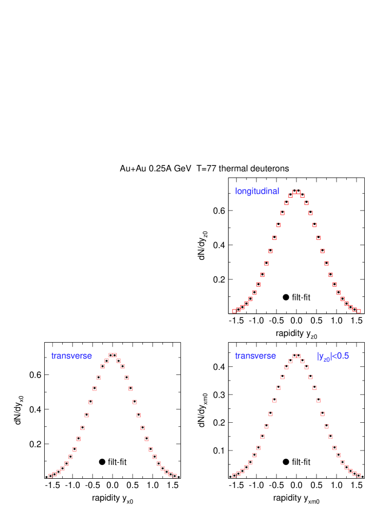
Figure 1: Rapidity distributions of deuterons in Au+Au reactions at $0.25A$ GeV obtained from a thermal model with $T=77$ MeV. The original predictions are given by (red) open squares, the reconstructed distributions after filtering and then extrapolating are given by (black) filled dots. The upper left panel shows the filtered distribution in scaled momentum versus rapidity space, the various color tones corresponding to yields differing by a factor 1.5. The lower panels show the integrated (left) and the constrained transverse rapidity distributions, while the longitudinal distribution is plotted in the upper right panel.

4.2 Tests of passage to $4\pi$ using IQMD

The following example shows the application to a case which cannot be a thermal distribution since it is the superposition of the three isotopes (p, d, t) of hydrogen. As can be seen from Fig. 2, there are three separate contributions to the phase space distribution after applying the filter: they are from the CDC, the Helitron and the Zero Degree detectors. We show both the experimental data and the simulation with IQMD. Pion contributions are excluded or subtracted using the information obtained in [38].

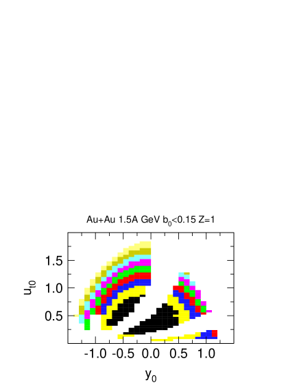
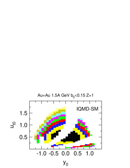
Figure 2: Distributions $dN/du_{t0}dy_{0}$ of hydrogen fragments emitted in central collisions of Au+Au at $1.5A$ GeV. The various color tones correspond to cuts differing by factors 1.5. The distributions are filtered by a sharp-cut filter the left panel showing the experimental data, while the right panel shows the simulation (applying the same centrality and filter cuts) with IQMD.

The reconstruction of the full acceptance rapidity distribution of the simulation causes no difficulty as demonstrated in Fig. 3. The existence of low $p_{t}$ data due to the Zero Degree proves to be a very useful constraint on the reconstruction.

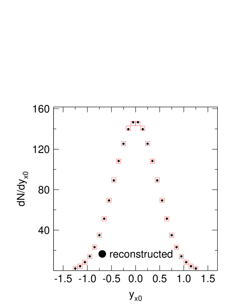
Figure 3: IQMD simulations: Longitudinal (upper panel), transverse and constrained transverse rapidity distributions of hydrogen fragments emitted in central collisions of Au+Au at $1.5A$ GeV. The original predictions are given by (red) open squares, the reconstructed distributions after filtering (see Fig. 2) and then extrapolating are given by (black) filled dots.

The acceptance for identified protons in the higher energy runs was more restricted since the Zero Degree detector did not allow isotope separation and the need to use the Helitron in addition to the Plastic Wall restricted the forward part of the detector somewhat. This is shown in Fig. 4. Still, we find that the reconstruction, for central collisions (which are of prime interest here) is very satisfactory.

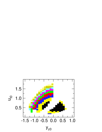
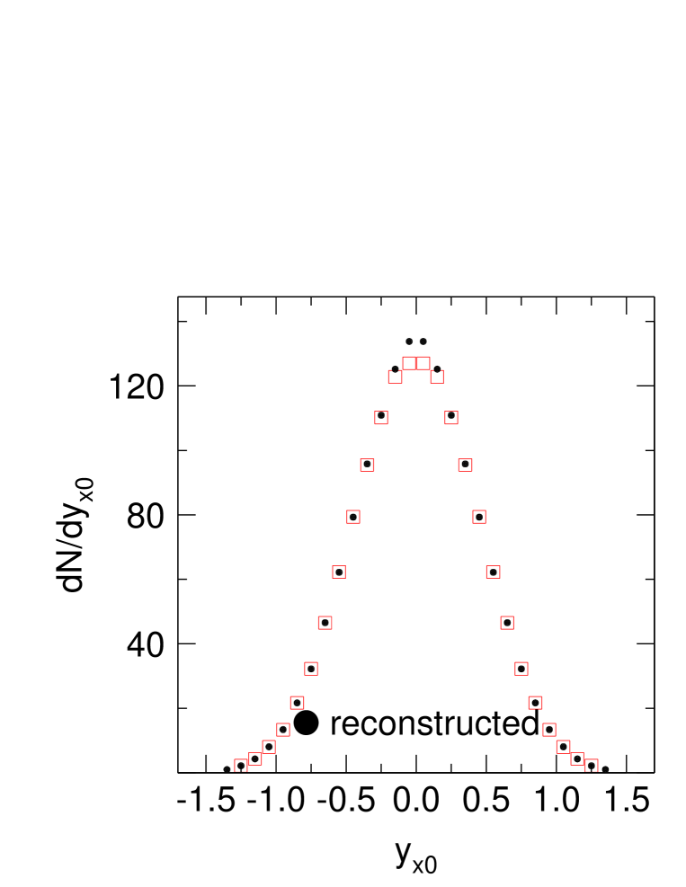
Figure 4: Rapidity distributions of protons in Au+Au reactions at $1.5A$ GeV obtained from IQMD-SM. The original predictions are given by (red) open squares, the reconstructed distributions after filtering and then extrapolating are given by (black) filled dots. The upper left panel shows the filtered distribution in scaled momentum versus rapidity space.

A case with a typical ’isotope acceptance’ (for deuterons here) in the low energy runs, where only the CDC was available for isotope separation, is shown in Fig. 5. With the sharp filter distorted phase space cells near $y_{0}=-1$ due to multiple scattering effects in the target are also cut out. Due to missing low $p_{t}$ information and despite the mentioned constraints from the more complete data on $Z=1$ fragments, the reconstruction has to allow for about $7\%$ errors indicated by the plotted systematic error bars. The accumulated counts in the experiment were actually 10 times higher than in the shown IQMD simulation, so that uncertainties originating here also from finite statistics were smaller in the experiment. On the other hand, again, the relatively faithful $4\pi$ reconstruction is limited to central collisions, where low $p_{t}$ spectator material is not so copious. Here the sum-of-isotopes check proved to be mandatory to make sure there was no ’extrapolation catastrophe’. Constraints from charge separated data obtained with the ZERO Degree Detector, covering low transverse momenta, were used for these checks.

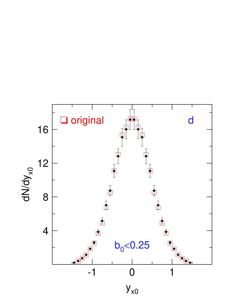
Figure 5: Rapidity distributions of deuterons in Au+Au reactions at $0.15A$ GeV obtained from IQMD-SM. The original predictions are given by (red) open squares, the reconstructed distributions after filtering and then extrapolating are given by (black) filled dots. The upper left panel shows the filtered distribution in scaled momentum versus rapidity space.

4.3 Heavy clusters

The $4\pi$ reconstruction of fragments with $Z>2$, that we call here ’heavy clusters’ (hc) is somewhat problematic due to the more limited acceptance, although the two-dimensional extrapolation procedure is an improvement over the conventional one-dimensional extrapolation with separated rapidity bins. The results presented here for hc, see also ref. [34], should be considered to be estimates when applied for example to $90^{\circ}$ spectra. In Fig. 6 we show an illustrative picture of what it meant to ’reconstruct to $4\pi$’. A stringent test using IQMD was not possible here due to limited statistics available for hc in the simulation. However, observables, such as stopping, relying on $4\pi$ coverage, were found to be in very reasonable agreement with INDRA data [33]. As can be seen by inspecting Fig. 6, the increased ’stopping’ at an incident energy of $0.25A$ GeV as compared to $0.09A$ GeV (larger transverse momenta relative to the longitudinal ones) is already suggested before the extrapolation.

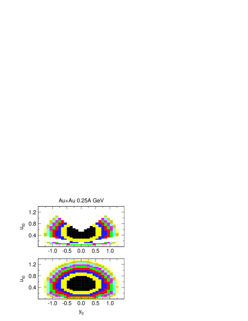
Figure 6: Example of $4\pi$ reconstruction of the phase space population for $Z=3$ fragments in central ($b_{0}<0.15)$ Au+Au collisions at two indicated incident energies. The upper two panels show the measured part after applying some smoothing, a sharp filter cut and reflection symmetry, the lower two panels show the result of a two-dimensional extrapolation to $4\pi$ geometry.

4.4 Adjusting the low-energy runs to high energy runs

As mentioned in section 2, the CDC was operated in split mode in the low energy runs, i.e. with a different voltage, [24], on the inner wires. Despite careful calibration to take this into account, it turned out by comparison with later runs made without the split voltage feature, that an additional correction was needed for the low energy runs. Fortunately this correction could be shown to involve just a simple rescaling factor. This is illustrated in Figs. 7 and 8 which consist both of two panels, the left one showing for central Au+Au collisions at $0.4A$ GeV differences of the two operating modes (the earlier one with split voltage) before, and, in the right panel, after correction with a constant rescaling factor. Fig. 7 shows kinetic energy spectra for protons, while Fig. 8 shows transverse rapidity spectra for tritons. A common sharp filter is applied to the data from both experiments. The two peak-structure in Fig. 8 is a consequence of the limited acceptance, see the example in Fig. 5. The rescalings in both figures 7 and 8 was primarily along the abscissa, the rescaling of the ordinates then followed from the condition that the integrated yields were not affected.

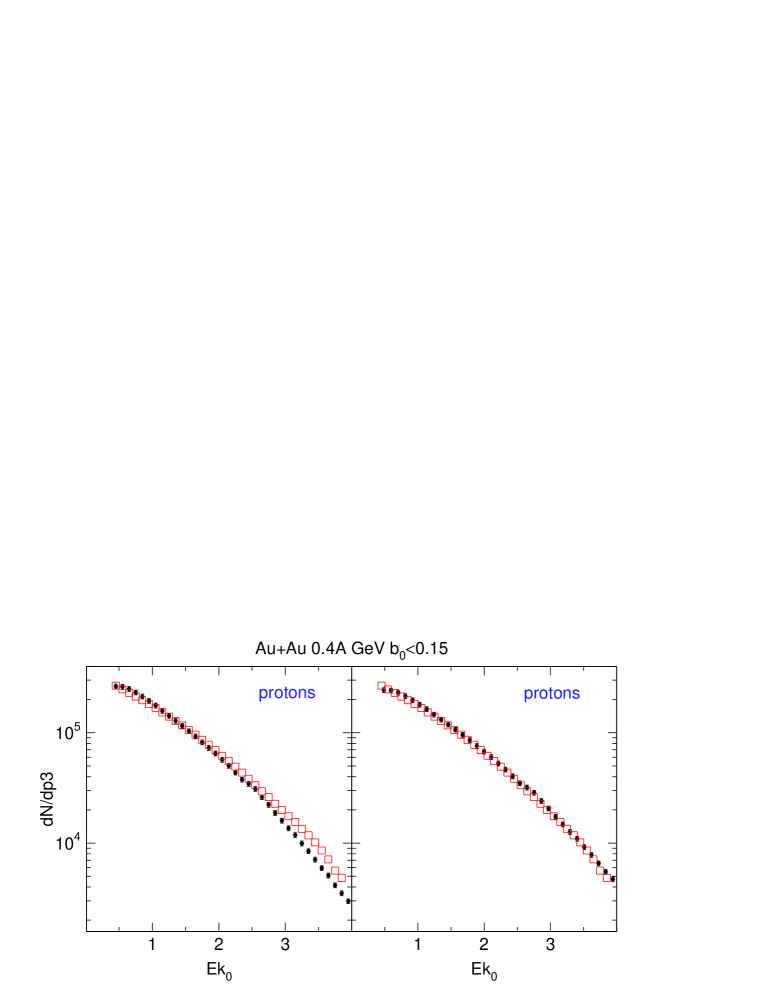
Figure 7: Left panel: kinetic energies (scaled units) of protons emitted at $90^{\circ}$ in central collisions of Au+Au. Comparison of two experiments performed in the low energy (full black circles) and the high energy campaigns (red squares). In the right panel the low energy experiment is rescaled along the abscissa by a factor 1.1 to achieve agreement with the high energy experiment.

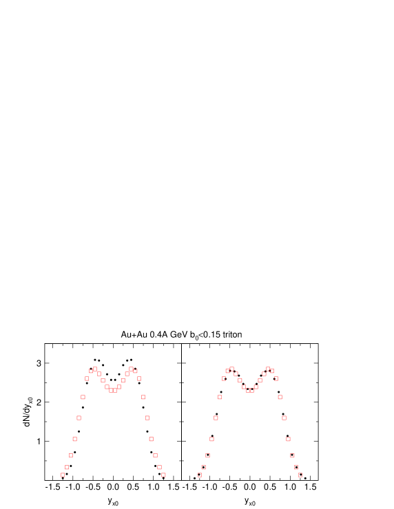
Figure 8: Sharp filtered transverse rapidity distributions for tritons in central Au+Au collisions at $E/A=0.4A$ GeV. Comparison of two experiments performed in the high energy (open red squares) and the low energy campaigns (full black circles). Left panel: original data. Right panel with the low energy data rescaled by factor 1.1 along the abscissa.

To avoid too many arbitrary parameters, the rescaling factors were fixed for all the low energy data down to $0.09A$ GeV. An example of the resulting extremely smooth behaviour of excitation functions for average kinetic energies covering the complete data is shown in Fig. 9. As will be shown later, this surprisingly regular trend is also predicted by IQMD simulations. We use scaled energy units here: a value equal to one indicates an energy equal to the incoming c.m. kinetic energy per nucleon. The figure also shows the reasonable agreement with data from ref. [42] which were obtained by our Collaboration using a different method. While we show here only a comparison for protons for reasons of space economy, similar conclusions hold for all other isotopes of hydrogen and helium.

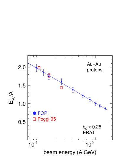
Figure 9: Average kinetic energy (scaled units) of protons emitted around $90^{\circ}$ (c.m.) in central collisions of Au+Au as a function of incident beam energy. The straight line fitted to the combination of the low/high energy data (logarithmic abscissa) reproduces, after correction of the low energy data, the individual points with an average accuracy of $1.2\%$. The data of [42] (red squares) are also shown.

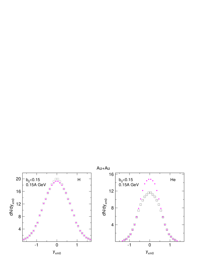
Figure 10: Left panel: Constrained transverse rapidity distribution of H fragments in central Au+Au collisions. (Black) open squares: demanding Z identification only, (pink) closed circles: sum of identified isotopes (p, d, t). Right panel: same for He.

4.5 Z-renormalization

By Z-renormalization we address the sum-of-isotopes check and correction after $4\pi$ reconstruction, which uses the fact, shown earlier, that we had a more complete acceptance for fragments identified by charge only. This was most important for the low energy runs. We illustrate the necessary ’renormalization’ in Fig. 10 for hydrogen and helium isotopes in central collisions of Au+Au at $0.15A$ GeV. While renormalization is seen to be only a small effect for hydrogen, the worst case scenario shown for helium requires a significant correction for low transverse velocities, which can be traced back to errors due to not accounting properly for Coulomb repulsion effects on low momenta not covered by our data.

5 Rapidity distributions

We present the phase space distributions in a way which deviates somewhat from the traditional way: instead of showing standard (longitudinal) rapidity distributions on a linear ordinate scale and then switching for the transverse direction to transverse momentum distributions on a logarithmic scale, we show the transverse degree of freedom in the same representation as the longitudinal degree of freedom, namely in terms of transverse rapidities plotted on a linear scale as well (see definitions in section 3). This allows to compare more directly longitudinal and transverse directions, a recurrent theme in the present work which is much concerned with assessing the degree of stopping and equilibration in these complex central collisions. We shall also be interested in the constrained transverse rapidity distributions (defined in section 3) which are likely to be closest to thermalized distributions.

$4\pi$ phase space distributions of five ’light charged particles’ (LCP: p, d, t, ³He,⁴He) have been reconstructed using four different centralities in 25 system energies, i.e. 500 2d-spectra are available. This number could be doubled if we consider that two different selection criteria (ERAT and MUL, see section 3) were applied throughout. However, unless otherwise stated, we shall show generally only the ERAT selected data. Further, for $E/A\leq 0.4$ GeV we have the data for heavier charge separated clusters (typically up to Z=8) and for $E/A\geq 0.4$ GeV charged pion data of both polarities (see [38]). It is out of question to present here all this rich information. Instead we shall present samples which serve to illustrate some of the typical aspects of the LCP data and add a few remarks on heavier clusters and pion data [38]. In later sections some of these aspects will be summarized in terms of simple concepts: ’stopping’, ’radial flow’ and ’chemistry’. These concepts reflect the time sequence of the central reactions. Earlier work on these aspects will be referred to.

Some of the rapidity distributions will be compared with distributions expected from a Boltzmann thermal model. These thermal distributions are generated varying T until the variance of the constrained transverse rapidity distribution (i.e. with the scaled longitudinal distribution constrained by $|y_{z0}|<0.5$ and within the $y_{xm0}$ range shown in the respective panels) is reproduced (the same constraints are used on the thermal simulation). The obtained T will be dubbed ’equivalent’ temperatures, $T_{eq}$. The longitudinal constraint leads to a cutoff of part of the yields, a cutoff which is particle-mass and T dependent. This cut is corrected for when extracting so called effective ’mid-rapidity yields’ from the experimental data by comparison to the thermal model (see section 8).

5.1 Light charged particles (LCP)

The next two 4-panel figures, Figs. 11, 12, show the three kinds of rapidity distributions for protons emitted in the most central Au+Au collisions at two incident energies differing by one order of magnitude: $0.15A$ GeV and $1.5A$ GeV.

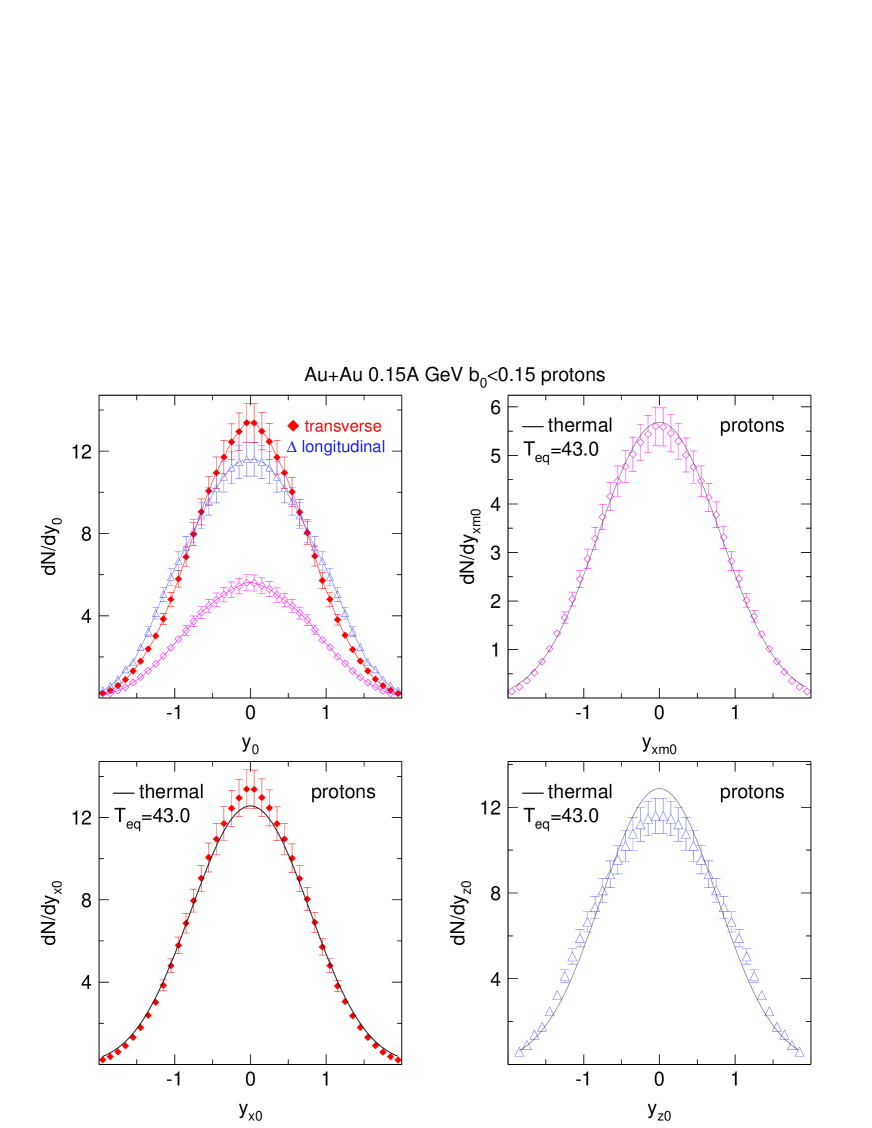
Figure 11: Upper left panel: Longitudinal (blue open triangles) and transverse rapidity distributions (red full diamonds) of protons in central collisions of Au+Au at $0.15A$ GeV beam energy. The third, lower yield curve (magenta open diamonds) in the panel represents the ’constrained’ transverse rapidity distribution: here a cut $|y_{z0}|<0.5$ on the longitudinal rapidity is applied. The smooth curves are just guides for the eye here. In the other three panels the three kinds of distributions are compared to a thermal distribution (corresponding to an equivalent temperature of 43 MeV) having the same area as the respective data, but a variance as implied by the constrained transverse distribution (seen in upper right panel).

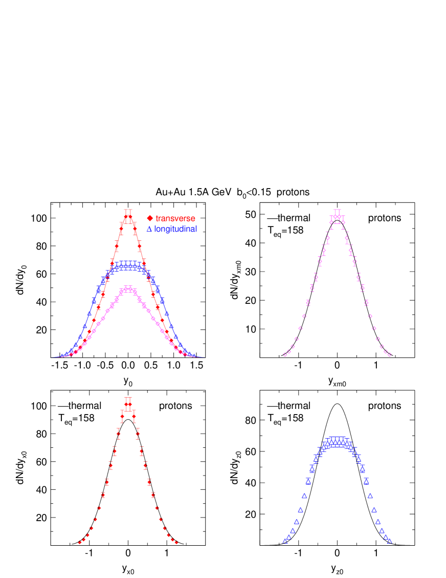
Figure 12: Upper left panel: Longitudinal (blue open triangles) and transverse rapidity distributions (red full diamonds) of protons in central collisions of Au+Au at $1.5A$ GeV beam energy. The ’constrained’ transverse rapidity distribution is also shown: here a cut $|y_{z0}|<0.5$ on the longitudinal rapidity is applied. The data points are joined by smooth curves to guide the eye. In the other three panels the three kinds of experimental distributions are compared to a thermal distribution (smooth black curves) having the same area as the respective data and a variance as implied by the constrained transverse distribution (seen in upper right panel).

The upper-left panels in the two figures show that the longitudinal rapidity distributions are broader than the transverse distributions, but while the effect is relatively modest at the lower energy, it is more conspicuous at the higher energy. The constrained transverse distributions are generally somewhat broader than the integrated transverse distributions and can be reproduced rather well by a thermal model simulation having an adjusted ’equivalent’ temperature, $T_{eq}$, and the same total area. We find $T_{eq}=43$ MeV, and $158$ MeV, respectively, for protons at the two energies. This $T_{eq}$ comes closest to the ’inverse slopes’ usually fitted to $p_{t}$ spectra in the literature, but is different in the sense that it is obtained by just demanding a reproduction of the bulk experimental variances taken in the shown rapidity ranges and hence excluding far out tails of the distributions. On the linear scales applied in the figures one finds a very satisfactory reproduction of the shape of the $dN/dy_{xm0}$ distributions (upper right panels). A comparison to the equivalent thermal representations fixed from the constrained data, to the full transverse and longitudinal distributions in the lower panels stresses the differences to the naive thermal expectations. The full transverse distributions are modestly narrower only, but the longitudinal distributions clearly deviate.

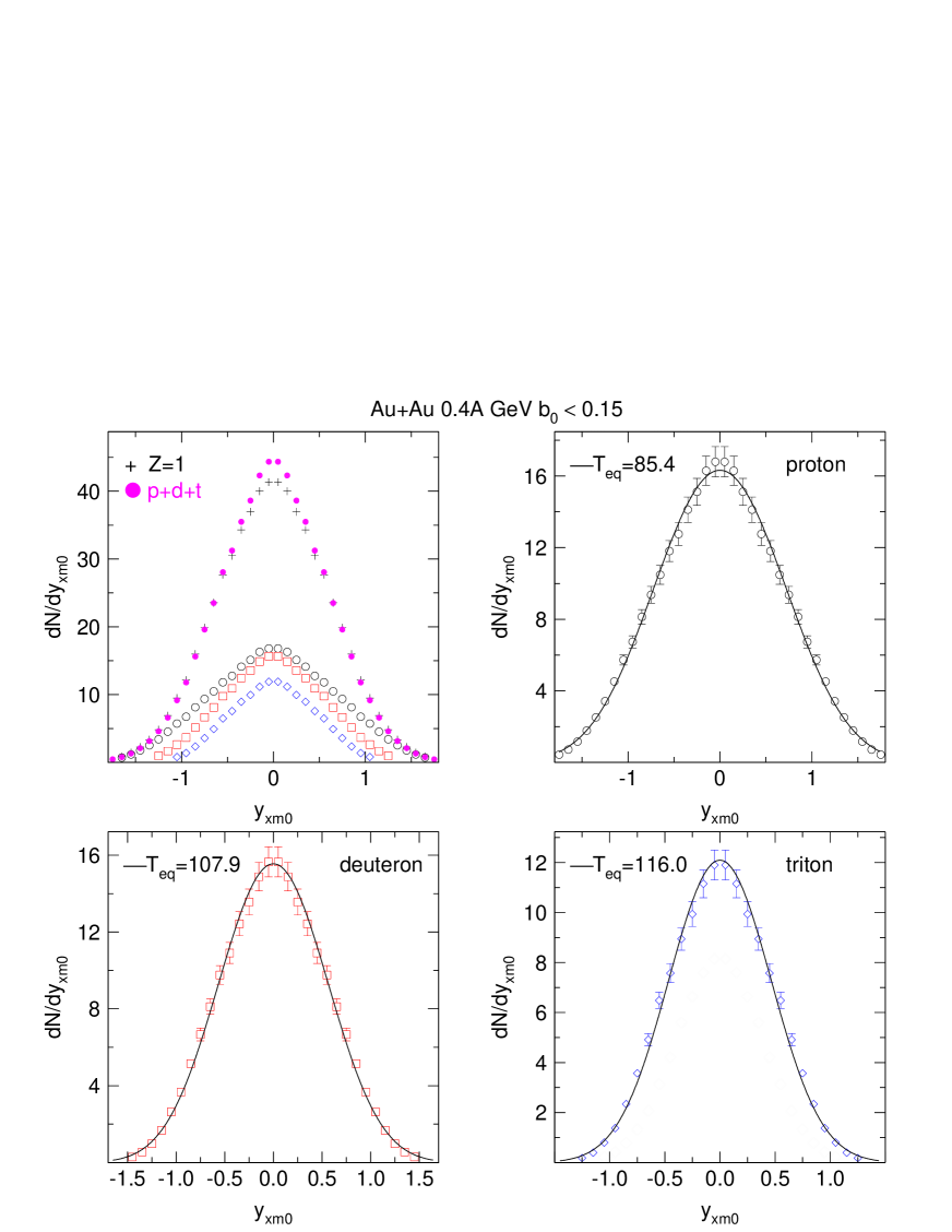
Figure 13: Central ($b_{0}<0.15$) Au+Au collisions at 0.4A GeV. Comparison of experimental scaled and constrained transverse rapidity distributions $dN/dy_{xm0}$ of protons (upper right), deuterons (lower left) and tritons (lower right) with thermal distributions (smooth black curves) assuming the indicated equivalent temperatures $T_{eq}$. The upper left panel shows the distributions of the three H isotopes, their sum (pink full dots) and the distribution for Z=1 (excluding created particles) obtained requiring only charge identification.

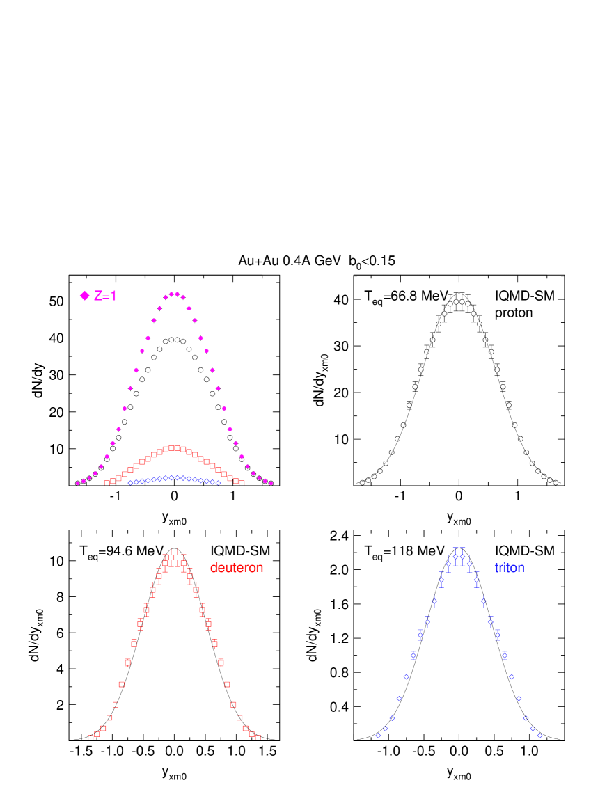
Figure 14: Central ($b_{0}<0.15$) Au+Au collisions at 0.4A GeV. Comparison of simulated (IQMD-SM) scaled and constrained transverse rapidity distributions $dN/dy_{xm0}$ of protons (upper right), deuterons (lower left) and tritons (lower right) with thermal distributions (smooth black curves) assuming the indicated equivalent temperatures $T_{eq}$.

The next two 4-panel figures, Figs. 13, 14, take a closer look at constrained transverse rapidities varying the (hydrogen) isotope mass. The system is Au+Au at $0.4A$ GeV with $b_{0}<0.15$. First we show the data, then a simulation with IQMD. In each case we make in the upper left panel the sum-of-isotopes check (which is fulfilled by definition in the simulation) and we compare in the other panels with a thermal model calculation adjusting $T_{eq}$. These one-shape parameter fits are close to perfect, but require a rising equivalent temperature with the isotope mass, a well known phenomenon often interpreted as ’radial flow’ in the literature that we shall come back to in section 7. Clearly there is no global equilibrium, but at very best a ’local’ equilibrium (in the hydrodynamic sense).

A closer look at the simulated data reveals small but systematic shape differences that exceed those found when using experimental data instead of the IQMD events. One could argue that the experimental data look more ’thermal’. Note the rather strong decrease of yields with isotope mass in contrast to the more comparable yields in the experiment shown in the previous figure. Also, if one were to associate, naively, the strength of radial flow with the mass dependence of $T_{eq}$, then one would conclude that the simulation overestimates the flow somewhat, since, as indicated in the various panels the $T_{eq}$ rise from 85 MeV for protons to 116 MeV for tritons in the data, while for the simulation we find 67 MeV and 118 MeV, respectively. For further discussions of the $T_{eq}$ values, see later section 7.

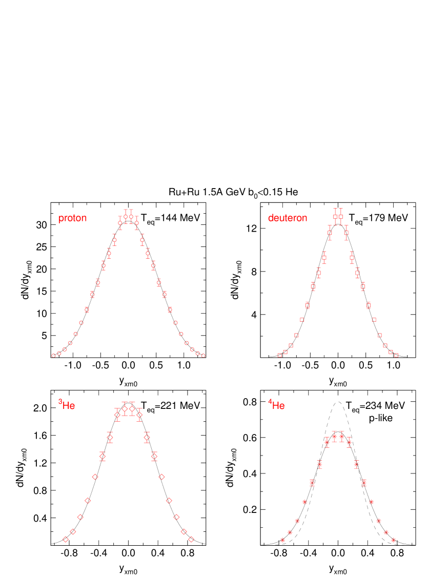
Figure 15: Comparison of experimental constrained transverse rapidity distributions $dN/dy_{xm0}$ with thermal distributions (black smooth curves) having the same first and second moments in central collisions of Ru+Ru at $1.5A$ GeV. The various ejectiles and the equivalent temperatures $T_{eq}$ are indicated. In the lower right panel we also plotted the ⁴He distribution (dashed smooth curve, ’p-like’) expected if the equivalent temperature was the same as for protons, but with the integrated yields unchanged.

The Fig. 15 showing constrained transverse rapidity distributions for central collisions in the system Ru+Ru at 1.5A GeV serves two purposes: 1) besides hydrogen isotopes (p and d) it also shows data for ³He and ${}^{4}He$ in the lower panels. Again thermal model calculations with the indicated $T_{eq}$ are shown along with the data; 2) We show that the ⁴He data are not well represented by a coalescence model using the measured proton data as generating spectrum: see the dashed curve. Indeed the observed rising equivalent temperatures with mass contradict the naive model. This is at variance with ref. [43] where the validity of the power law for a wide range of incident energies and centralities in Au+Au systems was stressed. The authors mentioned that a cutoff of $p_{t}/A$ smaller than 0.2 GeV/c was required and that the single (’free’) proton spectra had to be used, rather than the total spectra including those bound in clusters as one would naively expect. Non-perturbative features of clusterization are suggested strongly by our data, as we shall show later in this section and in section 8.

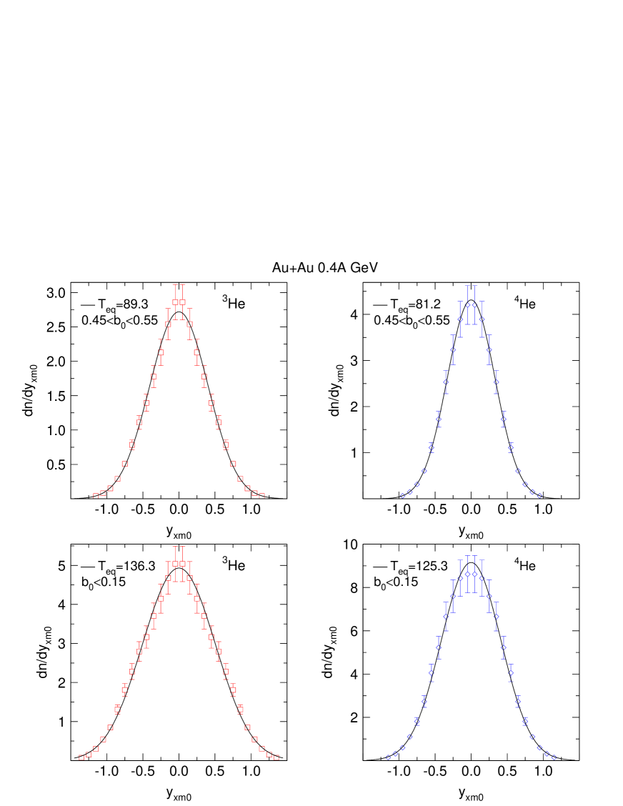
Figure 16: Central ($b_{0}<0.15$) (bottom) and semi-central (top) Au+Au collisions at 0.4A GeV. Comparison of experimental scaled and constrained transverse rapidity distributions $dN/dy_{xm0}$ of ³He (left) and ⁴He (right) fragments with thermal distributions (smooth black curves) assuming the indicated equivalent temperatures $T_{eq}$.

In the cases shown so far we observe a regular rise of $T_{eq}$ with the mass of the ejectile. However, frequently in the literature, the so-called ’helium anomaly’ is mentioned [44], namely the observation that ³He kinetic energies are not lower, but higher than the ⁴He energies, a phenomenon that to our knowledge has not been reproduced by microscopic dynamic reaction models. In Fig. 16 we show for Au+Au that even at the relatively high incident energy of $E/A=0.4$ GeV this phenomenon still subsists to some degree as the $T_{eq}$ for ⁴He are not found to exceed those of ³He. Further we show in the panels the rather strong drop of $T_{eq}$ with decreasing centrality, which is varied from $b_{0}<0.15$ (lower panels) to $0.45<b_{0}<0.55$ (upper panels). This is a general feature also observed at other energies and was reported earlier [45].

5.2 The influence of clusterization

The failure of the naive coalescence approach consisting in trying to reproduce the spectra of heavier clusters from the measured nucleon (proton) spectra (Fig. 15) and some of the ’He-anomaly’ discussed before may be connected with our current failure to understand clusterization quantitatively on a microscopic level (compare also the upper right panels of Figs. 13 and 14). Concerning the probability of nucleons to cluster, we are at SIS in a non-perturbative regime (see section 8): heavier cluster formation has a back-influence on the lighter generating transverse rapidity spectra.

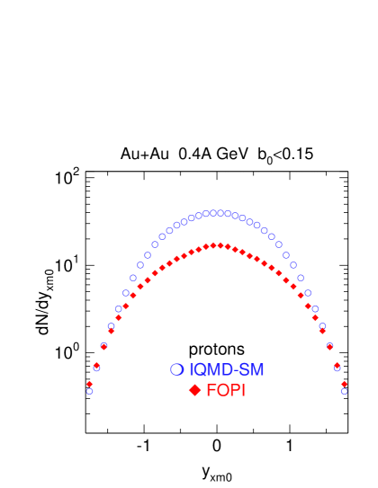
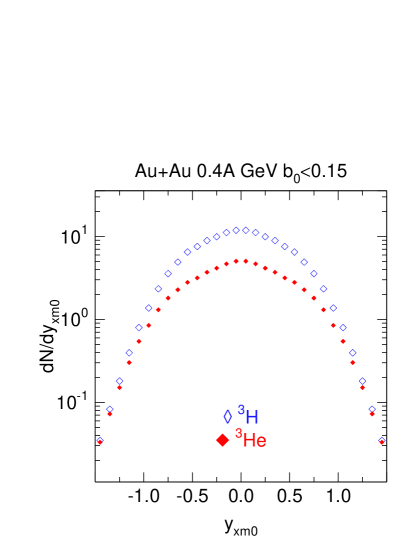
Figure 17: Left panel: Constrained transverse rapidity distributions of protons in central collisions of Au+Au. Comparison of data (red closed diamonds) and IQMD simulation (blue open circles). Right panel: comparison of experimental data for ³He (red closed diamonds) and ³H (blue open diamonds) in the same reaction.

The two-panel Fig. 17 illustrates the non-perturbative features at SIS. In the left panel we show the remarkable difference between FOPI and IQMD for the transverse rapidity distributions of protons. The surplus of IQMD for lower transverse velocities or momenta is due to a lack of sufficient clusterization: in the experiment more copious cluster formation massively depletes the low momenta. The right panel compares two experimental distributions: now it is the ³He that appears to have its low momenta depleted relative to ³H (the naive perturbative coalescence model does not predict any difference here). In view of the finding of the left panel, it is tempting to associate the effect to the formation of heavier clusters from the ’primeval’ ³He (created in earlier expansion stages).

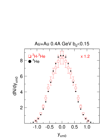
Figure 18: Comparison of the difference spectrum (see right panel previous figure) ³H-³He (rescaled by a factor 1.2) to the ⁴He (black dots) transverse rapidity spectrum.

This conjecture is supported by Fig. 18 which shows the ³H-³He difference spectrum together with data for ⁴He. The ³H and the ³He compete to be a condensation nucleus to a possible ⁴He. If both mass 3 isotopes are in a neutron-rich environment, the ³He will ’win’ for two reasons:
a) it is easier to ’find’ a single neutron to attach to ³He than a single proton to attach to ³H;
b) in contrast to ³H, the ³He nucleus does not Coulomb-repulse its needed partner.
A quantitative transport model theory must include the formation of $\alpha$ clusters if these conjectures are correct.

5.3 How to define stopping: varxz

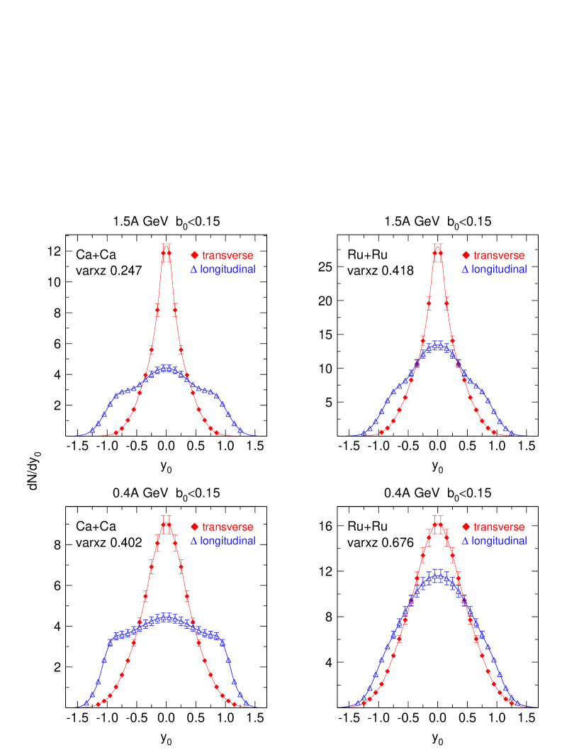
Figure 19: Comparison of scaled rapidity distributions for deuterons in central collisions at $E/A=1.5$ GeV (top panels) and 0.4 GeV (bottom panels): shown are data for Ca+Ca, Ru+Ru and Au+Au (from left to right). In each panel, the scaled longitudinal rapidity $y_{z0}$ distributions (blue open triangles) are shown together with the scaled transverse rapidity $y_{x0}$ distributions (red). The derived value of the stopping observable varxz is also indicated.

The final figure in this section on rapidity distributions, Fig. 19, serves to illustrate what we shall call ’partial transparency’ or ’incomplete stopping’. Transparency increases as either the studied system mass is lowered, or the incident energy is raised by going from $E/A=0.4$ GeV (lower panels) to 1.5 GeV (upper panels). With this figure, which shows data for the most central collisions ($b_{0}<0.15$ or $2.2\%$ of the equivalent sharp cross section), we argue that a good measure of the degree of stopping consists in evaluating the ratio varxz of variances varx and varz of the transverse relative to the longitudinal rapidity distribution, respectively, both of which are shown in the figure for deuterons. Note also the subtle evolution of shapes, especially at the higher energy: there is no trivial subdivision into ’participants’ or ’spectators’ possible. The interpretation in terms of two remnant counterflowing (not completely stopped) ’fluids’ is strongly supported by isospin tracer methods (see section 6) and suggests that not only global, but also local equilibrium is not achieved.

6 Stopping

As introduced in section 5.3, we quantify the degree of stopping by comparing the variances of transverse rapidity distributions (defined in section 3) with that in the longitudinal $(z)$ direction. Throughout we use scaled rapidities (i.e. the rapidity gap is projected unto the fixed interval $(-1,+1)$) and typical samples have been shown and discussed already (section 5). All rapidities are evaluated in the c.m.. However, for the ratios we discuss the scaling is immaterial. We shall call varxz the ratio of the variances in the $x$-direction and the $z$ direction. The choice of x is arbitrary, i.e. it is not connected with the azimuth of the reaction plane. varxz(1) is defined like varxz except that the integrations for calculating the variance are limited to the range $|y_{z0}|<1$; in [32] this was called vartl and $|y_{x0}|$ was also constrained to be $<1$. Such a restricted measure of stopping can be more adequate if measured data outside the range $|y_{z0}|<1$ are missing or less reliable. For varxz(0.5) the transverse rapidity distribution is taken under the constraint $|y_{z0}|<0.5$ on the scaled longitudinal rapidity. This measure of stopping is clearly biased and has systematically higher values, but is of interest when comparing with many data in the (higher energy) literature, where often attention is focused on transverse momentum spectra around (longitudinal) midrapidity. When no number in parenthesis is given, the intervals in rapidity are sufficiently broad to make the value of varxz asymptotically stable within the indicated, mostly systematic, errors.

There are other ways of characterizing stopping. Videbaek and Hansen [46] have introduced the mean rapidity shift $<\delta y>$ which is defined by

$$<\delta y>\equiv\frac{\int_{-\infty}^{y_{cm}}|y-y_{tgt}|(dN_{p}/dy)dy}{\int_{-\infty}^{y_{cm}}(dN_{p}/dy)dy}$$

where $y_{cm}$ is the rapidity of the c.m., $y_{tgt}$ is the target rapidity and $dN_{p}/dy$ is the proton rapidity distribution (a similar formula exists relative to the projectile rapidity $y_{p}$ with the integration limits interchanged). This observable was also determined in some works of our Collaboration, [48, 49]. The inelasticity K was used by NA49 [47] and is defined by $K=E_{inel}/(\sqrt{s}/2-m_{p})$ with $E_{inel}$ being equal to the average energy loss of incident nucleons with rest mass $m_{p}$. The common feature of these definitions is that one assesses stopping relative to initial conditions: the conclusion is then that a high degree of stopping is reached in collisions all the way up to at least SPS energies, especially if it is assessed in terms of energies. Our stopping variable has a different goal: we want to assess the difference relative to a completely stopped scenario, an assumption that is frequently assumed in (one-fluid) hydrodynamic codes for heavy ion collisions because of its inherent simplicity of a needed starting point of the calculation. Our observable, varxz, is important to assess the partial memory of the original (accelerator induced) counterflow of two fluids and hence deviations from local equilibrium. It is also of value to help determine viscosity properties of nuclear matter [50].

6.1 Isospin tracing

We invariably find that longitudinal rapidity distributions are broader than transverse rapidity distributions, see section 5. In principle, for a given system, one cannot exclude that this phenomenon is caused by a rebound opposite to the incident direction after a complete stop. The system size dependence of the effect, see namely Fig. 19, can be used to strongly argue against this interpretation which would imply an unlikely stronger rebound in smaller systems. An alternative method to demonstrate partial transparency was introduced by our Collaboration [52] and consists in so called isospin tracing. We refer the reader to the original publication for further explanations. Briefly, we combine rapidity distribution information of four systems involving the isotopes ⁹⁶Zr and ⁹⁶Ru : Ru+Ru, Zr+Zr, Ru+Zr and Zr+Ru, where the mixed systems are merely technically different in the sense that beam and target are inverted.

In the following, abbreviating $N^{RuZr}_{y}(p)$ the rapidity distribution of protons in the reaction Ru+Zr, etc, we define
$R_{4y}(p)=[N^{RuZr}_{y}(p)-N^{ZrRu}_{y}(p)]/[N^{RuRu}_{y}(p)-N^{ZrZr}_{y}(p)]$
This observable is a slight variant of the observable $R_{Z}$ used in [52]: it is an average of the two opposite-sign branches obtained by switching target and projectile in the mixed system. An arbitrary (here negative) equal sign is defined (the two branches of $R_{Z}$ in the chosen symmetric-mass systems must be equal except for sign). In Fig. 20 we show $R_{4y}$ for central collisions at $0.4A$ and $1.5A$ GeV together with rapidity distribution plots. In case of complete mixing with loss of memory (both alternatives: rebound as well as partial transparency) of the incident geometry, the rapidity dependences of $R_{4y}$ should be flat at zero value. There is indeed a small flat part around $y_{z0}=0$, especially for the most central ($b_{0}<0.15$) selection, but for higher $|y_{z0}|$ there is an increasing deviation from zero, the sign of which can be unambiguously associated with transparency, rather than rebound. The effect is definitely more pronounced at the higher energy in full accordance with the information from the variances of the rapidity distributions (see the upper panels in the figure). Only statistical errors are shown in the lower panels of Fig. 20. A more detailed presentation and discussion of the new isospin tracing data will be published elsewhere [53].

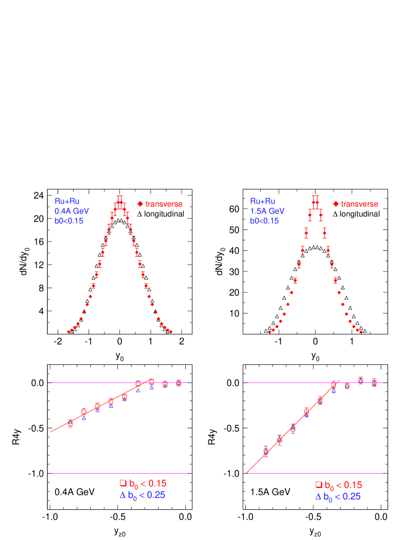
Figure 20: Top panels: Longitudinal and transverse rapidity distributions of protons in collisions of Ru+Ru at $0.4A$ GeV (left) and $1.5A$ GeV. Bottom panels: The corresponding $R_{4y}$ observables for two slightly different indicated centralities as a function of the longitudinal rapidity $y_{z0}$.

6.2 Global stopping and the EOS

By adding up the measured rapidity distributions of the different ejectiles one can try to obtain a global system stopping. The excitation function for Au on Au, first published in [32], was later slightly revised and combined with data from the INDRA collaboration [33]. The combined data are shown again in Fig. 21, but this time together with IQMD simulations using alternatively a hard ($K=380$ MeV, HM) or a soft ($K=200$ MeV, SM) EOS with momentum dependence [7]. As can be seen from the Figure, the difference between the HM and the SM simulation is significantly larger than the error bars in the data. This is an important observation as it opens up the possibility to observe EOS sensitivity also in central collisions in contrast to directed and elliptic flow which are linked to off-centrality (and in general collisions with less achieved compression). However, it is also clear that the ’residual’ interaction, i.e. the explicit collision term, influences the outcome. The present parameterization of IQMD as used here is obviously not able to reproduce the data, in particular the rapid drop of varxz(1) beyond $0.8A$ GeV is not reproduced. A fair reproduction of a portion ($0.25A$ to $1.0A$ GeV) of the excitation function was achieved in [50].

Clearly, varxz data should prove useful also to constrain the viscosity of nucleonic (and more generally of hadronic) matter if compared to transport model simulations. It is tempting to conjecture that the rising part of the excitation function is dominated by the decreasing importance of Pauli blocking as the rapidity gap exceeds the Fermi energy. Particle creation starts becoming important beyond $1A$ GeV [38] (see also our Fig.41 in the present work). But the decreasing trend of the varxz data seen in Fig. 21 suggests that this new channel does not compensate for the decrease and forward focusing of elastic nucleon-nucleon processes. The rapid decrease of varxz at the high SIS energy end is continued at AGS and SPS as we shall show later for net protons.

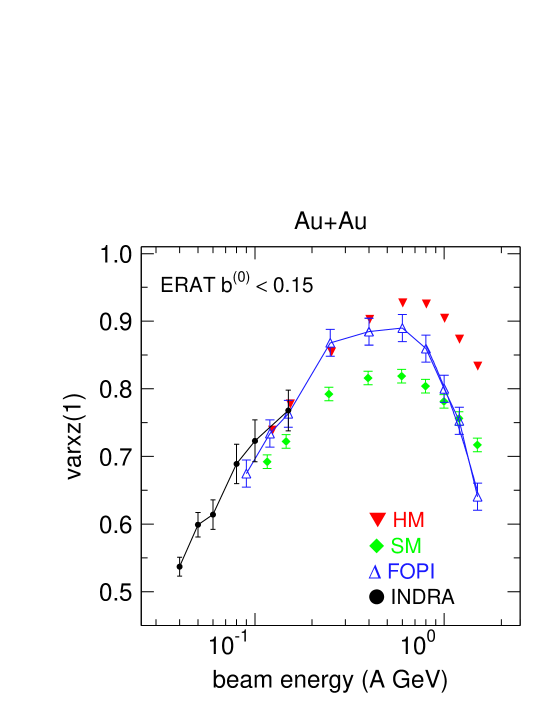
Figure 21: Excitation function of the stopping observable varxz(1) in central Au+Au collisions ($b_{0}<0.15$) [32, 33] . FOPI data: open blue triangles, INDRA data: black dots. These experimental data points are joined by straight line segments to guide the eye. IQMD simulations extending from $0.12A$ to $1.5A$ GeV: red full triangles (HM) and green full diamonds (SM).

6.3 p, d, t stopping: a hierarchy

By plotting varxz separately for identified fragments further insights (and constraints to simulations) can be gained. This is shown in Fig. 22. A remarkable feature is the similarity in the behaviour for the three isotopes, that suggests the collectivity of the phenomenon. There is a well defined maximum around $0.4A$ GeV for each of the isotopes qualitatively similar to the observed [32] global stopping. On the other hand a closer look reveals that there are some subtle differences in the shapes of the excitation functions. Except around the maximum, there is a hierarchy in the degree of stopping. This is illustrated in Fig. 23.

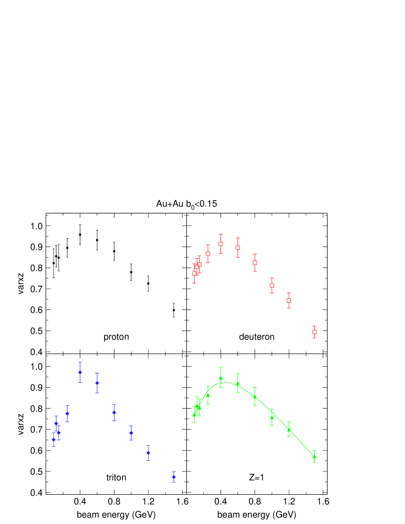
Figure 22: Excitation function of the stopping observable varxz in central Au+Au collisions ($b_{0}<0.15$). As indicated in the various panels the excitation functions are shown separately for the three hydrogen isotopes. The right-lower panel allows to compare relative to the average weighted Z=1 fragments. The smooth curve is just a polynomial fit.

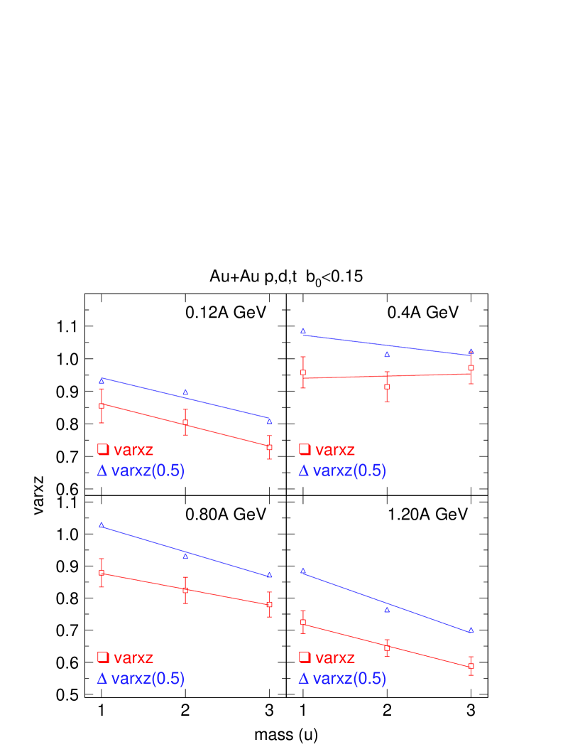
Figure 23: Mass number dependence of the stopping observable varxz of hydrogen fragments in central Au+Au collisions ($b_{0}<0.15$). Data are shown for 4 representative energies indicated in the panels (notice the one order of magnitude span). For comparison data are also shown for the ’constrained’ stopping observable varxz(0.5) (blue open triangles, error bars omitted). The lines are linear fits.

On the average clusters have ’seen’ less violent (less stopped) collisions when the stopping is incomplete for single emitted nucleons (away from the maximum around $0.4A$ GeV). This effect may be a surface effect but is not a ’trivial’ spectator-matter effect, as the rapidity distributions in these most central collisions do not exhibit well defined ’spectator ears’ around $|y_{z0}|=1$: there are no spectators in the strict sense here. The constrained stopping varxz(0.5) (blue open triangles in the figure) is always somewhat larger because the transverse rapidity distributions are broadened when a cut around longitudinal rapidity is applied. The trends with mass number and incident energy are similar however.

6.4 System size dependence of stopping

As remarked earlier, the system size dependence of the observable varxz is an important constraint to the question of transparency versus rebound dominated collision scenario, especially when only the most central collisions are compared in scaled units of centrality. All our data support transparency dominance. This does not mean that the degree of stopping is small, but it is significantly less than expected from ideal one-fluid hydrodynamics.

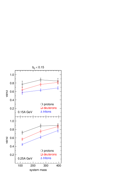
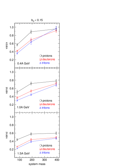
Figure 24: System size dependence of varxz for protons (black circles), deuterons (red squares) and tritons (blue triangles) at various indicated beam energies.

Figure 24 shows a rather complex behaviour and will be a challenge to ambitious microscopic simulations. One remarkable feature is the apparent saturation of varxz at a relatively low value for the highest incident energy. This was already seen earlier, [32], for global stopping. This suggests the beginning of a phenomenon seen in a more spectacular way recently at the SPS [47] ($E/A=158A$ GeV): at midrapidity there is no non-trivial increase of population in Pb+Pb relative to p+p collisions.

6.5 Isospin and stopping

One expects isospin dependences because the free nucleon-nucleon cross sections $\sigma_{nn}$ and $\sigma_{np}$ are different and also because the mean fields, shown earlier to influence global stopping, are expected to be isospin dependent. However the data show no convincing effect considering the error limits. This is shown in Fig. 25 where a comparison of two systems with the same mass, but different composition (Ru+Ru, $N/Z=1.182$ and Zr+Zr, $N/Z=1.400)$ is shown. In this context it is interesting to note that very recently a similar observation was made [51] at lower energies ($32-100A$ MeV) for Xe+Sn using various isotopes.

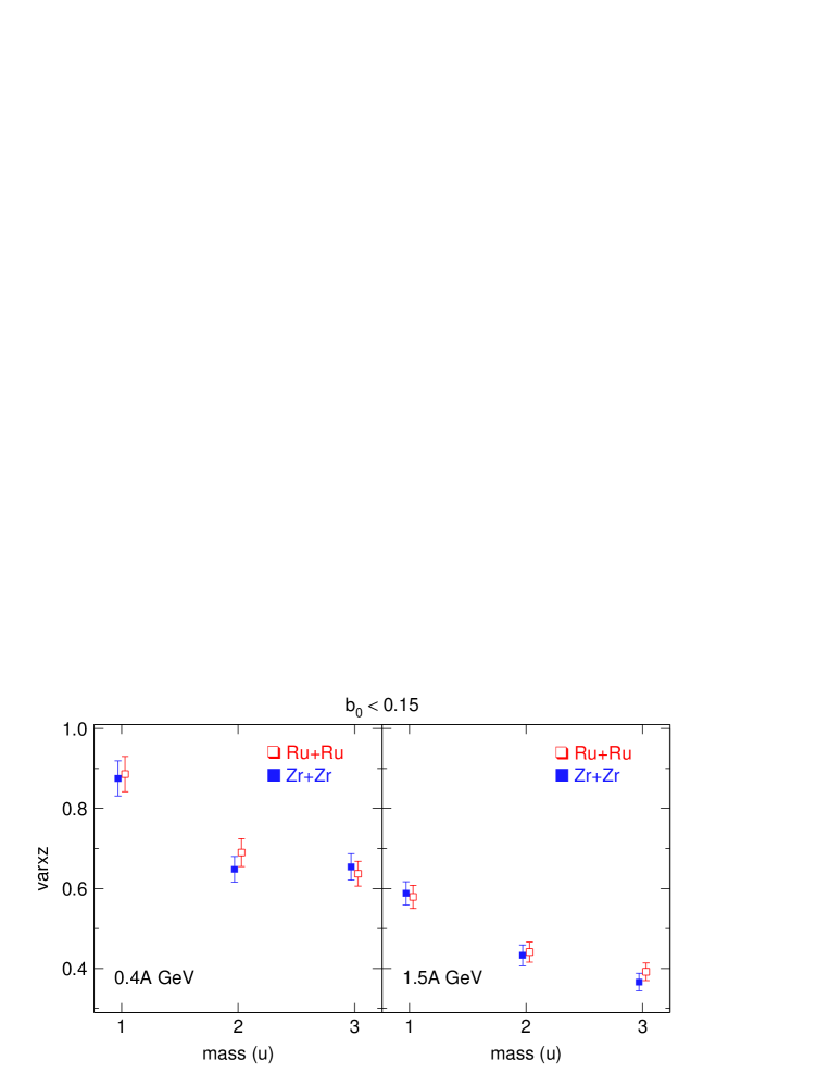
Figure 25: Mass dependence of varxz for hydrogen isotopes in central ($b_{0}<0.15$) Ru+Ru and Zr+Zr collisions at incident beam energies of $0.4A$ GeV (left panel) and $1.5A$ GeV (right panel).

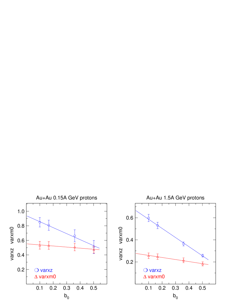
Figure 26: Centrality dependence of proton stopping ($varxz$) and mid-rapidity constrained scaled transverse variance ($varxm0$) at 0.15 and $1.5A$ GeV.

6.6 Centrality dependence of stopping

For comparisons with simulations it is useful to check how sensitively the observable varxz reacts to matching the centrality correctly with that of the experiment. The relatively strong dependence of varxz on centrality $b_{0}$ is illustrated in Fig. 26 for Au+Au at two rather different incident energies. The linear fits allow to estimate a limit for $b_{0}=0$. Since varxz is the ratio of varx and varz (the zero suffix is immaterial here since the scaling cancels out ), it is interesting to explore what causes the strong centrality dependence. The figure also illustrates the comparatively modest change of the scaled variance, varxm0 of the constrained transverse rapidity distribution (which we remind is obtained with a with a cut $|y_{z0}|<0.5$ on the scaled longitudinal rapidity).

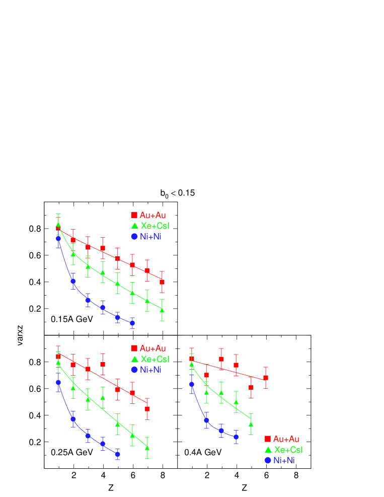
Figure 27: Charge number and system size dependence of the stopping observable varxz for fragments emitted in central Au+Au collisions ($b_{0}<0.15$). Data are shown for 3 representative energies and three systems indicated in the panels. The smooth curves, fitted to $a_{0}+a_{-1}Z^{-1}+a_{1}Z$, serve to guide the eye.

6.7 Heavy clusters

Since at lower energies we have been able to get information also for fragments with $Z>2$, we can extend the hierarchy of stopping to heavy clusters. The results are put together for three incident energies and three systems in Fig. 27. This confirms the existence of a stopping hierarchy in a very systematic way. Also a significant system-size dependence is evidenced. Note that the Z-dependence is flattest for Au+Au at $0.4A$ GeV, close to the maximum of global stopping shown before in Fig. 21. An extension, for $0.15A$ GeV, all the way to Z=20 using INDRA data has been shown earlier in [33], demonstrating also a reasonable consistency between data of FOPI and INDRA. Quantitatively, such data are presently outside the capabilities of microscopic simulations, but present a challenge for our theoretical understanding.

6.8 Joining up to higher energies

As mentioned at the beginning of this section, stopping at higher incident energies has not been characterized by varxz. The reason is connected with the increasing difficulty to measure and reconstruct the distributions $dN/dy_{z}$ and $dN/dy_{x}$ over the full range of rapidities that one needs to know. Often transverse momentum spectra in narrow $y_{z}$ bins, preferably around $|y_{z0}|=0$, are fitted individually to thermal ansatzes. We show therefore the ratio of variances using in the numerator the variance inferred from inverse slopes $T_{inv}$ determined from transverse momentum spectra in a bin $\Delta y_{z0}$ around (longitudinal) mid-rapidity. In terms of the notation introduced at the beginning of this section, this is likely to give an upper limit, varxz$(\sim 0.1)$, to the unconstrained varxz, as suggested by Fig. 23.

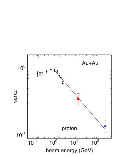
Figure 28: Excitation function of the stopping observable varxz for protons in central Au+Au collisions. In addition to FOPI data, obtained at SIS, we show here estimates from AGS (red full square) and SPS (blue full triangle) data. See text for further details.

With these restrictions in mind, we show in Fig. 28 an extension of our proton data on stopping to higher energies. The AGS (Alternating Gradient Synchrotron at Brookhaven) data point was constructed from ref. [54], the SPS (CERN Super Proton Synchrotron) data point from ref. [55] (NA49). A rather dramatic decrease of stopping, as defined in the present work, is evidenced, suggesting a fair amount of residual counterflow if one takes transverse fluctuations as scale. The straight line is a fit joining to SIS data starting at $0.6A$ GeV. However for the interpretation of stopping excitation functions of one specific particle, here protons, extending over more than three orders in the magnitude of the incident energy, it is important to realize that they can be misleading on the global system trend. The reason is that stopping hierarchies are omnipresent. At the low energy end protons are the most stopped particles, while at the high energy end net protons (the difference between protons and antiprotons) tend to be rather the least stopped particles. We are lead to expect stopping hierarchies in the higher energy regimes similar to the ones described here, but shall not pursue this as it would far exceed the scope of the present work. As consequence of incomplete stopping, the time the system spends at maximum compression (and heat) is shortened. This could prevent the full development of critical fluctuations expected theoretically in certain areas of the phase diagram.

7 Radial Flow

One of the first attempts to understand radial flow in central heavy ion collisions in the framework of microscopic transport theory was published in [56]. There, the transverse flow energy $E^{f}_{t}$ per nucleon was defined by

$$E^{f}_{t}=\int\!\!\int d\vec{r}d\vec{p}f[\frac{1}{2}m(v^{f}_{t})^{2}]/\int\!\!\int d\vec{r}d\vec{p}f$$

and the transverse flow velocity $v^{f}_{t}$ was calculated locally, using only those particles from the environment that have participated in the collisions and stopping the integration when the density $\rho_{0}/8$ was reached in the expansion stage ($f$ is the Wigner distribution function). Evidently this kind of radial flow is not a direct observable. Rather, it is usually inferred from the mass dependence of average kinetic energies of particles emitted around mid-rapidity (in cylindrical coordinates) or around $90^{\circ}$ c.m. (in spherical coordinates). This implies an interpretation of the data suggested by hydrodynamical thinking: the system’s quasi-adiabatic expansion leads to cooling, part of the energy being converted to (radial) flow. As we shall see this interpretation can be put to a critical test by studying the dependence of the apparent radial flow on the centrality and the system size and also by inspecting the correlation of the radial flow with the degree of clusterization taking the latter as a measure of the degree of cooling.

Relevant data for the SIS (or Bevalac) energy range have been published by Lisa et al. [45] and in a number of papers from our collaboration [40, 42, 48, 57, 58]. Azimuthal dependences of radial flow in the same energy range were studied in refs. [28, 30] and shown to be sensitive to the EOS, while little sensitivity was suggested for the azimuthally averaged radial flow.

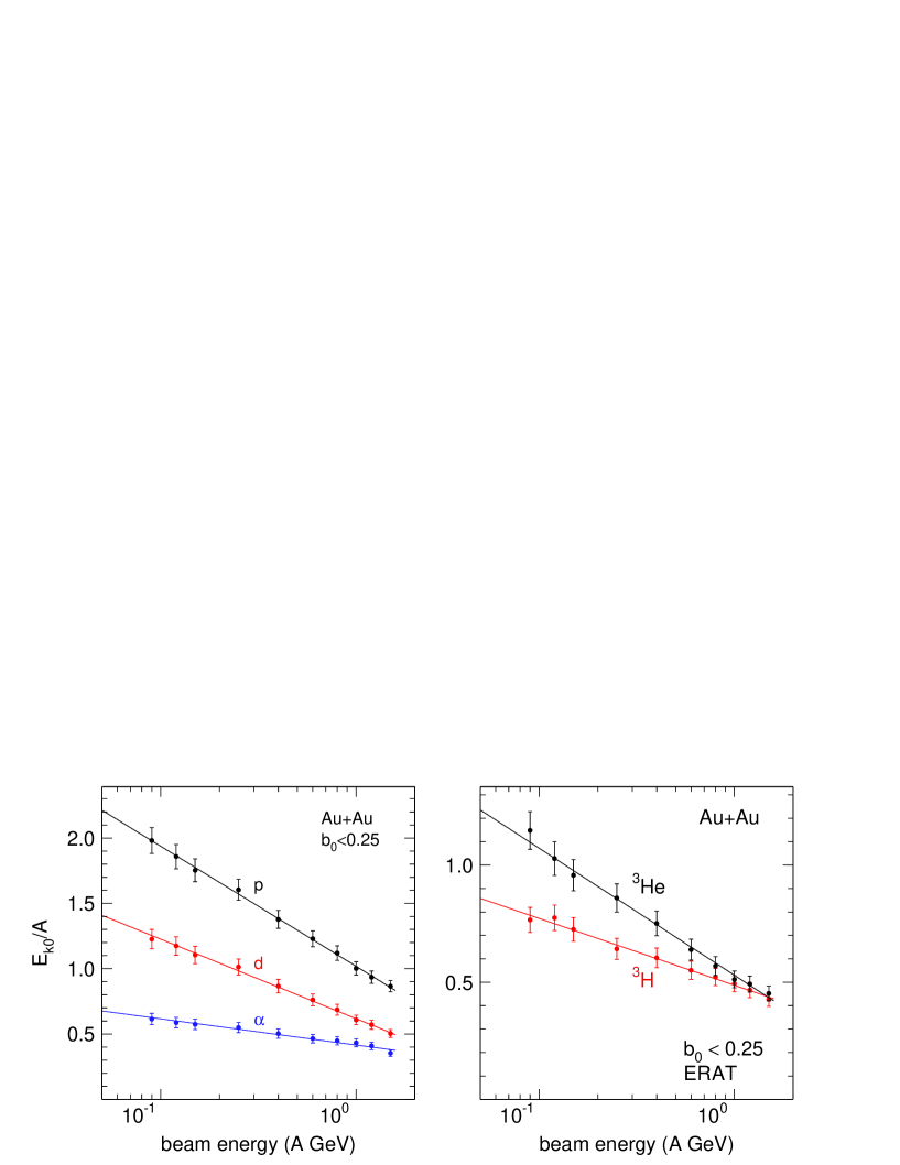
Figure 29: Average kinetic energy per nucleon (scaled units) of protons, deuterons and ⁴He (left panel) and of ³H and ³He (right panel) emitted in $90^{\circ}\pm 10^{\circ}$ in the c.m. in central collisions of Au+Au as function of beam energy. The excitation functions follow a linear dependence (straight lines) if plotted on a logarithmic energy scale.

We shall start by taking a look at the systematic evolution with incident energy and ejectile mass (hydrogen and helium isotopes) of average scaled kinetic energies per nucleon, $E_{k0}/A$. This is shown in Fig. 29 for collisions with $b_{0}<0.25$ and emissions into c.m. angles ($90\pm 10^{\circ}$). A striking feature is the extremely smooth evolution with beam energy: the point to point errors seem to be smaller than the indicated systematic errors. In these scaled units the energies gradually decrease as the available energy must be shared by an increasing number of emitted particles. The regularity suggests a very continuous change without any dramatic fast transition to some higher entropy phase. Note that at the low end we observe protons emitted perpendicular to the beam axis with on the average twice the incident beam energy per nucleon.

Another feature, demonstrated in the right panel of the figure is the difference between the two equal mass isotopes ³He and ³H. Starting at the low beam energy end with a difference of kinetic energies well in excess of the expectations from Coulomb effects [42], this difference gradually converges to zero in these scaled units. We have already discussed this ’anomaly’ in section 5 for the special case of an incident energy of $0.4A$ GeV and have given there a tentative interpretation. Here we see the ’anomaly’ apparently disappearing as production of clusters heavier than mass three drastically decreases (see also Fig. 43).

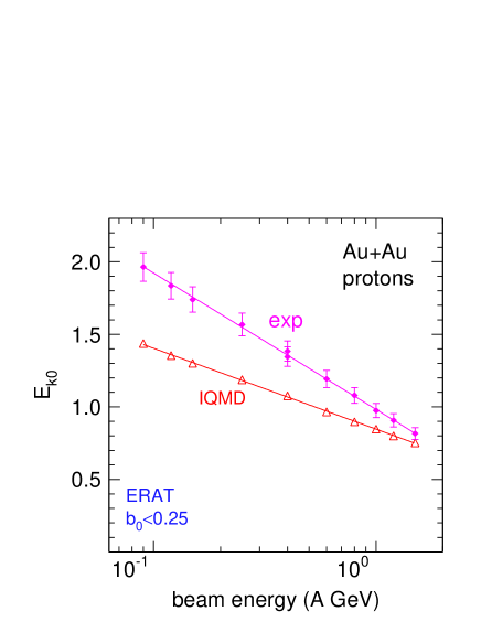
Figure 30: Average kinetic energy (scaled units) of protons emitted around $90^{\circ}$ c.m. in central collisions of Au+Au as function of the beam energy. Comparison of experimental data with simulations using IQMD-SM.

Another demonstration for the need to reproduce correctly the degree of clusterization in order to understand the kinetic energies of emitted particles is given in Fig. 30 for protons. Much like the experimental data the calculated data are reproduced with high accuracy ($0.7\%$) by a linear dependence on $\log(E/A)$. The slope characterizing the calculated trend is different however. The reason is connected with a lack of sufficient clusterization at the low energy end in the simulation. Too many single protons, together with the necessity to conserve the total energy (and mass), lead to smaller energy per nucleon. This stresses the need to reproduce the degree of clusterization for quantitatively correct comparisons with experimental observables pertaining to specific identified particles. In particular radial flow is connected with cooling leading to clusters. The two observables, cluster yields and radial flow, are therefore interrelated.

In Fig. 31 we show average kinetic energies of H and He isotopes emitted at $90^{\circ}$ c.m. in Au on Au collisions with centrality $b_{0}<0.25$. The data, plotted versus fragment mass for various incident beam energies, show pronounced structures that tend to decrease with incident energy: by adding INDRA data [59] for Xe+Sn at 0.05 GeV a very large range of incident energies is spanned. The structures prevent a straight-forward determination of a linear slope with mass that could be tentatively associated to a collective radial flow. The straight lines plotted in the various panels join the proton and deuteron data to the average kinetic energy of ${}^{3}He$ and ³H and ignore the ${}^{4}He$ data. As can be seen, the average mass three value continues the proton-deuteron trend with a remarkable accuracy, an observation that we found to be true for all studied system-energies and centralities (see also Fig. 37), allowing therefore to postulate a well defined observable, the slope of the corresponding straight line, that we shall call ’radial flow with the A3 method’, although this interpretation is clearly subject to caution.

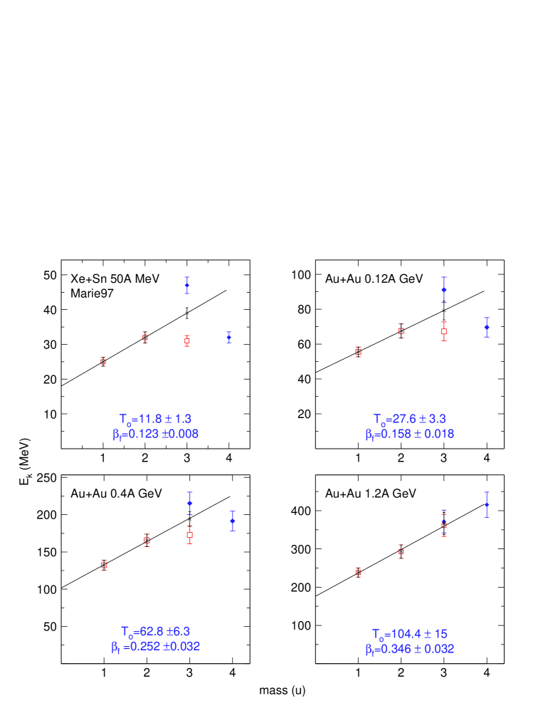
Figure 31: Average kinetic energies $E_{k}$ of H and He isotopes emitted at $90^{\circ}$ c.m. in Au on Au collisions with centrality $b_{0}<0.25$. Full (blue) diamonds: ^3,4He. The data are obtained at various indicated beam energies. The straight line is a linear fit up to mass 3. The data point at mass 3 ($\times$ symbol) was taken to be the average of ³H and ³He. The derived apparent temperatures, $T_{o}$, and (radial) flow velocities, $\beta_{f}$, are indicated. The upper left panel illustrates the use of the same method to INDRA data [59] for Xe+Sn taken at $50A$ MeV.

Defining $E_{k}=E_{f}\times A+E_{o}$ with $E_{f}=(\gamma_{f}-1)\,m_{N}$ ($m_{N}$ nucleon rest mass), we convert the mass slope $E_{f}$ from the just introduced A3 method to a (radial) flow velocity $\beta_{f}$ , derived from the average flow factor $\gamma_{f}$ , and the offsets $E_{o}$ in Fig. 31 to an ’offset temperature’ $T_{o}$ using relativistic formulae and ignoring mean field contributions to $E_{o}$ , in particular Coulomb fields. This allows us to compare to the analysis of [45], although the authors seem to have handled the data structures differently.

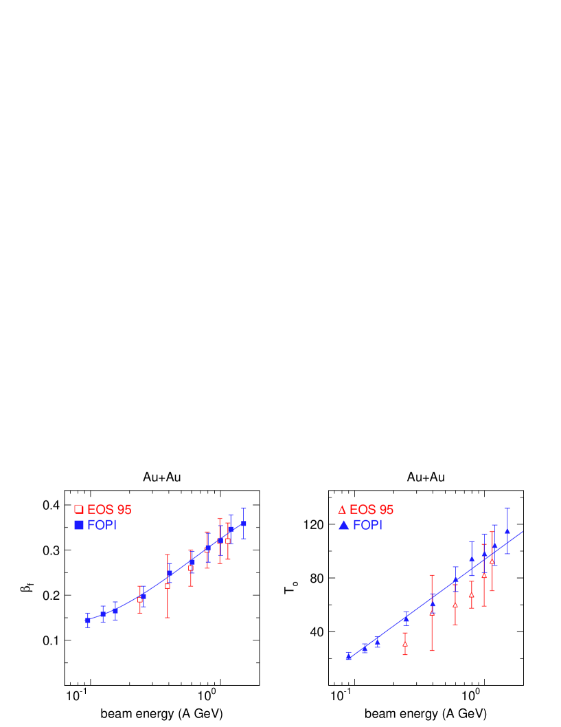
Figure 32: Radial flow velocities $\beta_{f}$ (left panel) and offset temperatures $T_{o}$ (right panel) for Au+Au collisions deduced from $90^{\circ}$ kinetic energies of mass 1-3 ejectiles ($A3$ method). The present data (blue full symbols) are compared to data from ref. [45]. The smooth curves are fitted to the present data only and serve to guide the eye.

This is shown in Fig. 32. The two datasets with nearly matched centralities are compatible, although our offset temperatures are systematically somewhat higher. Our data extend over a larger energy range and follow a more regular trend fixed by smaller error bars. The interpretation of the data in terms of a collective flow and a common ’local’ temperature is probably too naive: the stopping hierarchies evidenced in section 5 make a perfectly common flow improbable. We expect further the apparent offset $T_{o}$ parameters to be influenced both by Coulomb fields (especially at the low energy end) and by the repulsive nuclear fields built up by the compression (see Fig. 21).

7.1 System size dependences

In Fig. 33 we show the system size dependence of radial flow varying the incident energy by one order of magnitude. The increasing trend with system size is striking and characteristic for all energies. In each panel two sets of data are shown: the data points plotted with the open symbols and the larger error bars were obtained fitting two parameters separately to the data for one incident energy, the flow (slope) and the offset $T_{o}$. The second set of data points were obtained using a common offset $T_{o}$ indicated in the panel, a constraint allowing to fix the flow value better.

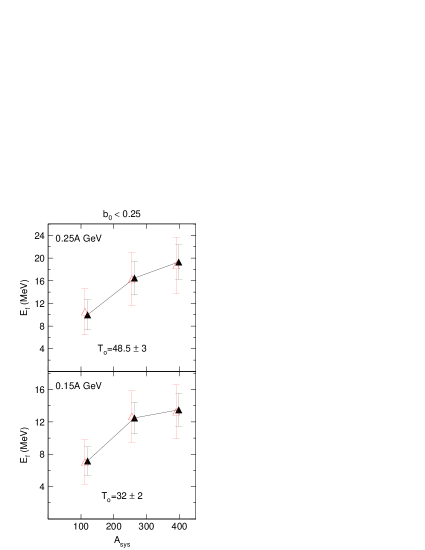
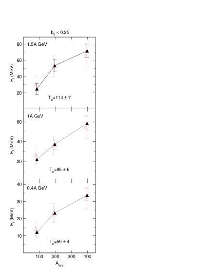
Figure 33: Radial flow energy in central collisions ($b_{0}<0.25$) as a function of system size. This observable is deduced from the mass dependence (A=1,2,3) of average kinetic energies at $(90\pm 10)^{\circ}$ c.m.. The open (red) data points are from separate fits (see previous figures) varying both the offset and the slope per mass unit (i.e. the flow parameter). The full (black) data points are obtained requiring a common offset parameter (indicated in the panels as offset temperature $T_{o}$). The incident beam energies, varied over one order of magnitude, are indicated in the upper left corner of each panel.

The difference between the two curves is small. However we find, when allowing two adjustable parameters for each system, that the $T_{o}$ values is not completely independent of the system size: from the lightest system to the heaviest (Au+Au) there is an increase by about $20\%$. This could be a ’relic’ of the repulsive mean fields due to increased compression in heavier systems. Unfortunately the uncertainty of $T_{o}$ is relatively large.

7.2 Comparison to IQMD

The observed system size dependence of the radial flow is not trivial: a comparison with the simulation using IQMD-SM, see Fig. 34, reveals that the strong dependence of the data on system size is not correctly reproduced. In [60], using IQMD, the authors conclude that radial flow is not sensitive to the EOS: they find that the sum of two contributions to this kind of flow, namely the mean field EOS and the nucleon-nucleon scatterings, tends to be the same for a stiff, resp. soft EOS. In the soft case the scatterings dominate because of the larger compression reached but this is compensated by the less repulsive mean fields. In view of the failure to reproduce the observed size dependence it is possible to question this conclusion. The increased production of clusters in larger systems, correlated with increased radial flow and stopping could well be a memory of the original compression (cooling by compression followed by expansion). In [34] it was found that softer EOS favours cluster formation at freeze out. This interpretation is supported by the theoretical work of ref. [61].

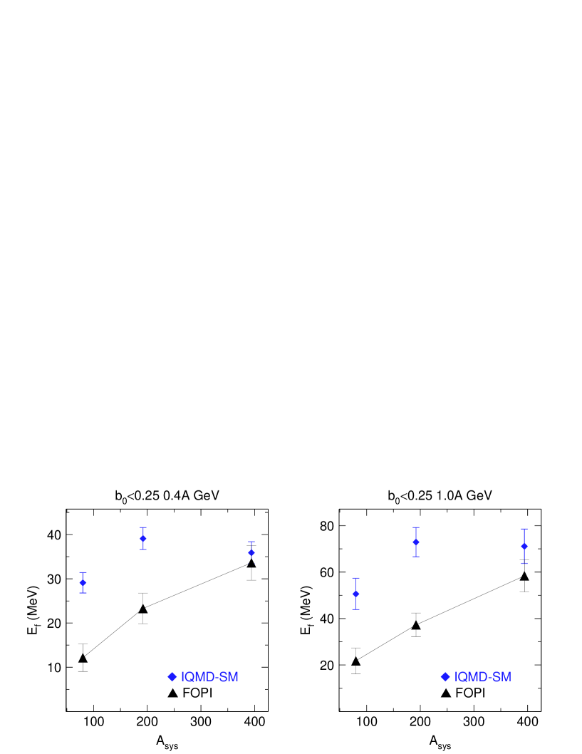
Figure 34: System size dependence of radial flow in central ($b_{0}<0.25$) collisions. The experimental data (black full triangles joined by straight lines) are compared with IQMD-SM predictions for $0.4A$ Gev (left) and $1.0A$ GeV (right) incident energies.

7.3 Heavier clusters

For incident energies below $0.4AGeV$ we were able to obtain data for fragments up to nuclear charge 6-8, depending somewhat on the incident energy. Although such data, not separated by isotope, and more limited in acceptance (see Fig. 6) have been published (’PHASE I’) and extensively discussed earlier by our Collaboration, [40, 57, 58, 62, 63], it is worthwhile to look again at these data in the light of the present more complete ’PHASE II’ information and new insights. The relevant information is summarized in Fig. 35 where we show the nuclear charge dependence of kinetic energies in central collisions of Au+Au for five incident energies varying from 0.09A GeV to 0.4A GeV. An earlier evaluation of these data, showing similar features, has been presented in [63]. The results cannot be compared directly: in ref. [63] a coordinate system rotated into the flow axis was used and in-plane fragments were suppressed. The datasets presented in each panel of Fig. 35, least squares fitted by a linear function, hold for c.m. polar angles of $(5-45)^{\circ}$ and $(80-100)^{\circ}$, respectively. To allow a more direct approximate comparison with the mass-dependent data discussed before, we have multiplied the measured kinetic energies per nucleon by $2Z$ and plotted them versus $2Z$. Obviously the slopes of the fitted lines (’$2Z$ method’) are very different for the two polar angle ranges (in agreement with [45]), but they tend to gradually align as the energy is raised (see upper right panel in the figure), a confirmation of the global trend of increasing stopping in this range of incident energies (Fig. 21). Increased stopping leads to a more isotropic distribution of kinetic energy, that was also visible for the light charged particles (Fig. 23, upper right panel showing the $0.4A$ GeV data). It is fair to remind at this stage, that while the data below $45^{\circ}$ are well covered by our acceptance, the data around $90^{\circ}$ are somewhat less reliable due to the necessity for a two-dimensional extrapolation (section 4). We are confident that the major conclusions are not seriously affected as, below $0.2A$ GeV, our analysis was found to be consistent with the more complete INDRA data [33].

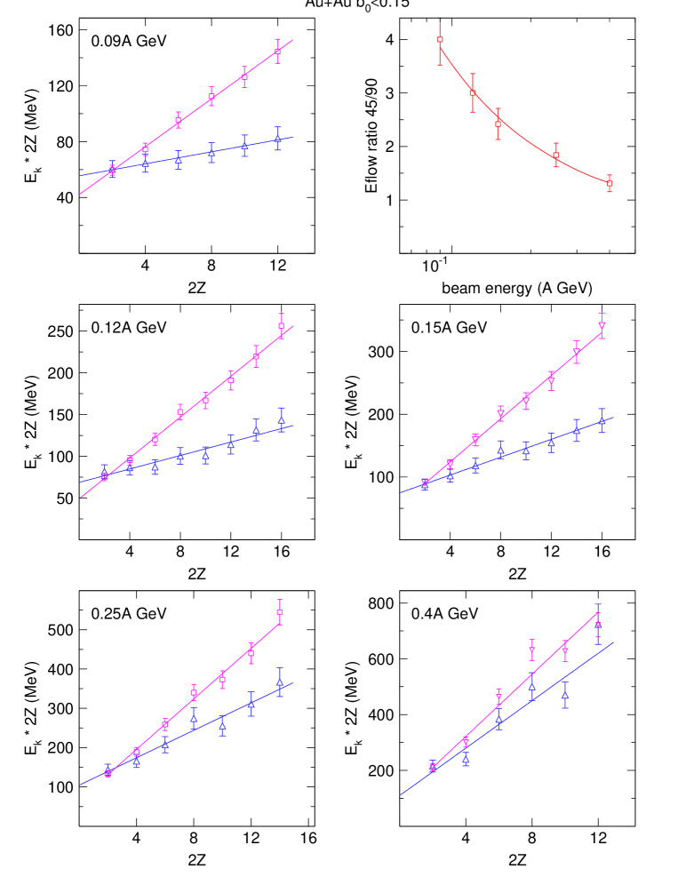
Figure 35: Nuclear charge dependence of kinetic energies for various indicated beam energies in central collisions of Au+Au. The measured kinetic energies per nucleon are multiplied by twice the nuclear charge (i.e. by $2Z$) and plotted versus $2Z$. Pink open squares: polar angles 5 to 45 degrees, blue open triangles: polar angles 80 to 100 degrees. The straight lines are linear fits. The upper right panel shows the ratio of the deduced slopes (i.e. ’flow’ energies) for the two types of polar angle intervals versus incident energy.

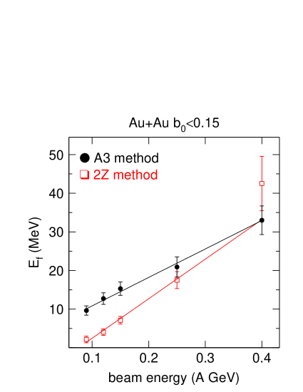
Figure 36: Radial flow versus incident kinetic energy. Comparison of analyses results obtained with $A3$ and with $2Z$ methods. The straight lines are linear fits.

It is interesting to compare the apparent radial flow deduced by the ’2Z method’, Fig. 35, with that deduced by the ’A3 method’, Fig. 31. This is shown in Fig. 36 for centrality $b_{0}<0.15$ (note that in order to match the centrality used in the analysis illustrated by Fig. 35, the centrality is higher than in Fig. 31 which is constrained to $b_{0}<0.25$ and therefore yields $E_{f}$ values lower by 4 to 7 $\%$). One sees the convergence of the two methods at $0.4A$ GeV where stopping is maximal, but at lower incident energies the A3 method yields higher values. We suggest to correlate this with the pronounced stopping hierarchy found at the lower energies (section 6). Clearly then, one needs to correct the apparent mass dependences for this effect when converting them to radial flow. This requires transport codes that reproduce the observed clusterization and stopping hierarchy.

At this stage we wish to make a comment to our flow analysis published in 1997, [40]. In the light of the present extensive information on incomplete stopping and hence strong deviations from isotropy, the earlier analyses assuming spheric expansion and neglecting partial transparency must be revised in the sense that the flow values found using the limited acceptance of the PHASE I of FOPI included a significant longitudinal (memory) component. Thus the analysis included some counter-streaming effects of the nucleons due to incomplete stopping (see Fig. 27). As the method used in [40] was strictly constrained by energy conservation, the sum of radial and two-fluid counter flow turned out to be correct, but the interpretation of the mass or charge dependence of the kinetic energies at these forward angles as just radial (spheric) flow cannot be upheld. The data themselves remain valid, except for a subtle effect on the topology of the two-dimensional ($u_{t}$ vs rapidity $y_{z}$) spectra: applying the ERAT criterion on the apparatus limited in PHASE I to laboratory angles forward of $30^{\circ}$ lead for the most central collisions (i.e. in the tails of the ERAT distributions) to an underestimation of the anisotropy as the selection criterion favoured events with a higher hit rate near the large angle apparatus limits, increasing the apparent isotropy. In the present work, with the significantly larger PHASE II acceptance, this effect, caused by event-by-event fluctuations, is minimized.

7.4 Sytematics of equivalent temperatures

In section 5 it was shown that the constrained rapidity distributions could be well reproduced with a thermal ansatz, giving an equivalent temperature $T_{eq}$. This represents an alternative way of systematizing mass dependences of phase space distributions. A systematics of $T_{eq}$ is shown in the next four figures that close this section. We find a similarity with the systematics of average kinetic energies of fragments emitted around $90^{\circ}$ : compare Fig. 31 with Fig. 37. However, since the phase-space cuts are different and the stopping is incomplete (non-spherical topology), the deduced parameters are not substitutes for each other. While we have started with $90^{\circ}$ kinetic energies primarily to join up to some of the earlier literature [28, 42, 45, 63], the $T_{eq}$ characterizing the constrained rapidity distributions allow us to join up to higher energy heavy ion data, including some of our own work [48], which are traditionally shown in (more appropriate) axially symmetric coordinate systems rather than spherical coordinate systems. The variation of $T_{eq}$ with particle type evidently excludes a naive interpretation in terms of a common (equilibrium) temperature. However, the observations illustrated in Figs. 11 to 16 go beyond just defining average kinetic energies since they allow a statement on the shapes of the distributions.

In Fig. 37 we show data for $0.15A$ GeV beam energy varying the system size. The same strong structures in the data for hydrogen and helium isotopes are visible and the A3 method introduced earlier, joining the proton and the deuteron $T_{eq}$ with the average of the two mass three (³He and ³H) data points is seen to define an accurate slope that can be again taken to quantify radial flow. The lower right panel allows to assess the system size dependence.

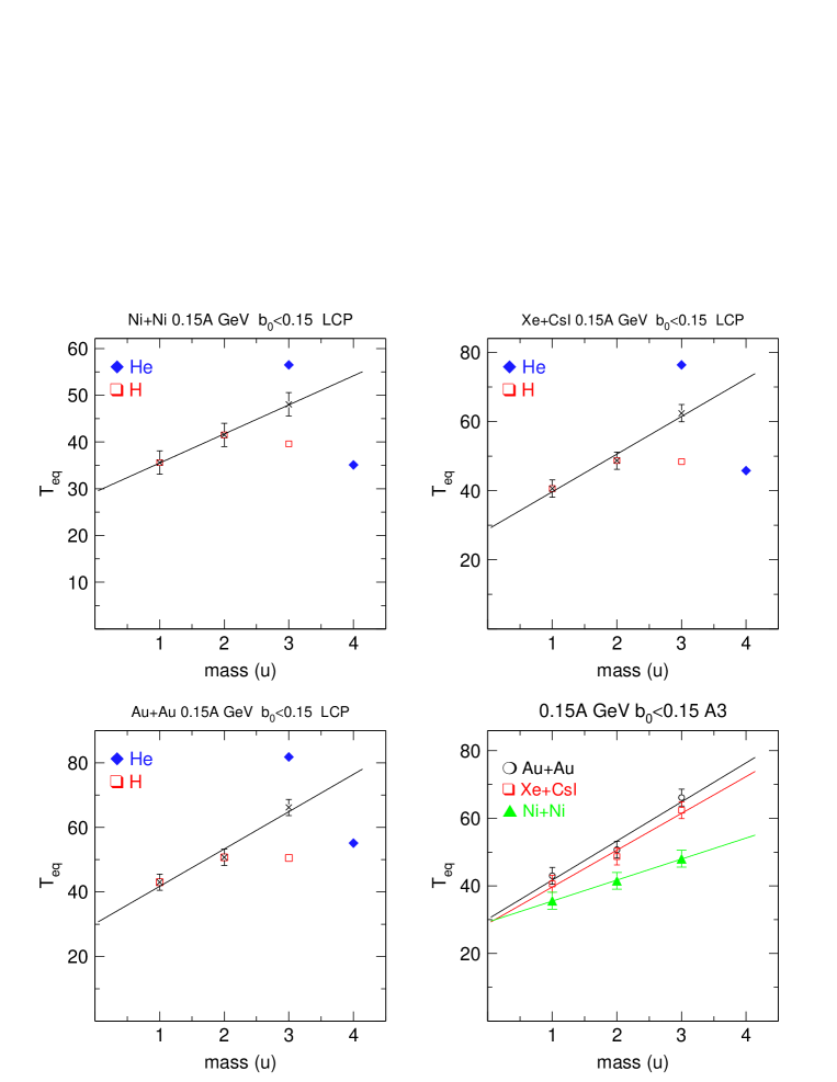
Figure 37: Equivalent transverse temperatures of hydrogen (open red squares) and helium isotopes (full blue diamonds) as function of their mass number in central Ni+Ni (upper left panel), Xe+CsI (upper right panel) and Au+Au collisions (lower left panel). A linear fit (A3 method) is also shown. The lower right panel allows to compare the three systems directly using the data points of the A3 method.

In Fig. 38 for data obtained at $1.0A$ GeV, we confront the systematics for hydrogen isotopes (left panel) with that for pions [38] of both charges. Note the strikingly different system size dependence of nucleonic clusters and of pions: while the $T_{eq}$ of pions slowly (the data are plotted with an ordinate offset) decrease with system size, the contrary is true for the hydrogen isotopes. Again, as suggested earlier, this is correlated to the different consequences of compression (creation of pions) and decompression-cooling (reabsorption of pions, creation of clusters from nucleonic matter).

Apparent temperatures for protons and deuterons in Ni+Ni collisions have already been published earlier by our Collaboration [48]. If we interpolate the data in Fig. 38 to estimate the Ni+Ni values we obtain $T_{eq}$ values exceeding those of [48] by about $15\%$. It is unlikely that the difference is due to a different analysis method. One possible explanation is the different methods used to select the most central collisions. In [48] the multiplicity was maximized between the polar laboratory angles $(7-30)^{\circ}$, while in the present work ERAT, determined using the full apparatus acceptance, was maximized.

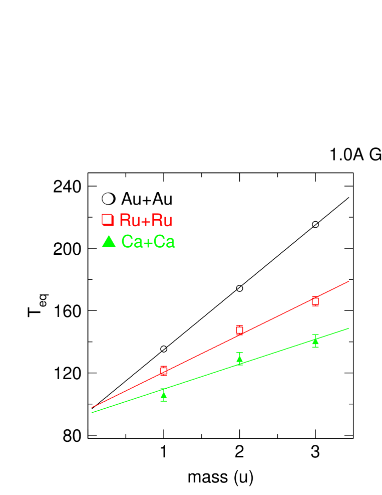
Figure 38: Equivalent transverse temperatures for symmetric central collisions at $1A$ GeV beam energy. Left panel: data for hydrogen isotopes versus mass for three indicated systems. Right panel: data for pions versus system mass. Note the tendency (for the hydrogen isotopes) to converge to a common apparent offset ’temperature’ $T_{o}$ (left) and the systematic difference between the two charged pions, as well as their weak decreasing trend as a function of $A_{sys}$.

In Fig. 39 we show an observation typical for the SIS energy range: the presence of cold spectator matter in non-central collisions tends to cool locally the participant matter. We compare collisions of different systems at the same estimated value $Apart$ of the participant matter. This effect can be studied in more detail by varying the angle relative to the reaction plane [28], but this will not be done here.

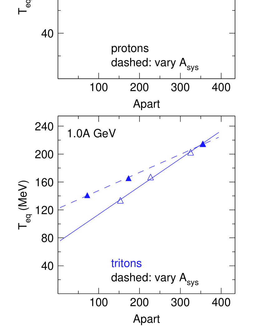
Figure 39: Equivalent transverse temperatures of protons (upper left panel), deuterons (upper right panel), tritons (lower right panel) and ³He as function of participant number $Apart$ for collisions at $E/A=1.0A$ GeV. The straight lines are linear fits. Open symbols and solid lines are for a variation of the impact parameter using Au+Au, full symbols and dashed lines are for a variation of the system size (Ca+Ca, Ru+Ru and Au+Au) at fixed reduced impact parameters ($b_{0}<0.15$).

Finally, we present in Fig. 40 for Au+Au at two different incident energies ($0.4A$ and $1.5A$ GeV) a complete systematics of $T_{eq}$ for all five LCP varying the centrality. From the smooth trends the limits for $b_{0}=0$ can be deduced. Note the inversion of the hierarchy for the two He isotopes when passing from the higher to the lower energy.

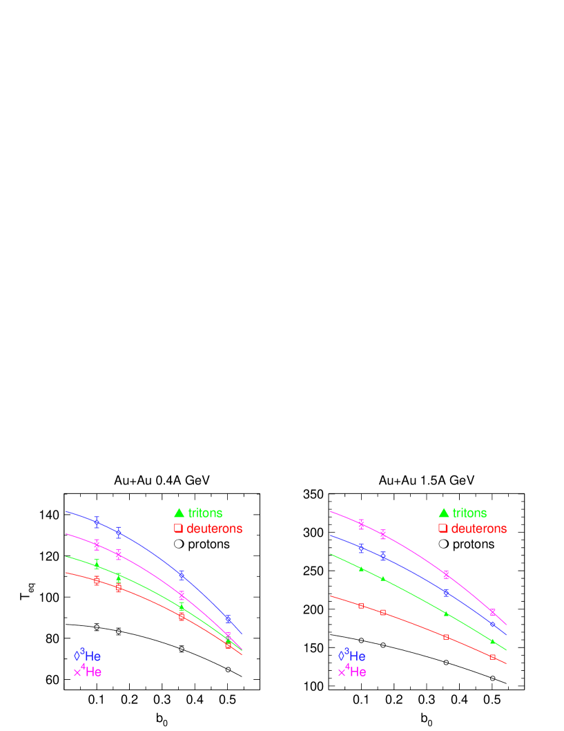
Figure 40: Centrality dependence of equivalent transverse temperatures for protons (circles), deuterons (squares), tritons (full triangles), ³He (diamonds) and ⁴He clusters in Au+Au collisions. Left panel: 0.4A GeV incident beam energy, right panel: 1.5A GeV. The smooth lines guide the eye and allow an estimate for $b_{0}=0$.

8 Chemistry

The $4\pi$ reconstructions, explained in detail in section 4, allow us to assess the integrated yields of all the ejectiles that constitute the bulk of the colliding system. For the most central collisions we present these yields in tabulated form in an appendix for the 25 system-energies studied in this work. Except for the two lowest incident energies ($0.09A$ and $0.12A$ GeV), we account for the total system charge with an accuracy of about $5\%$ or better. Note that we include in this balance also the pions, [38]. Other created particles, such as kaons etc, are negligible on the $5\%$ level (but are of course interesting for many other reasons). For the two lowest energies we miss significant contributions from heavy clusters beyond Z=8. The interested reader might consult INDRA-ALADIN works [33, 64, 65] for more complete distributions in the energy range at and below $0.15A$ GeV.

Such data are often analysed using models assuming (local) chemical equilibrium with a unique ’chemical’ temperature . An early, instructive presentation of the arguments in favour of a conjectured chemical equilibrium at freeze-out can be found in [66]. Even if one does not adopt the equilibrium assumption, (many of the observations presented in this work do not favour the equilibrium assumption) the degree of clusterization quantized by these yields can be used to constrain the outgoing (non-equilibrium) entropy [62, 67]. This information, together with our extensive data on stopping, section 6, can be used to assess the viscosity to entropy ratio that is currently intensely investigated in connection with the quark-gluon phase thought to be copiously produced at the highest currently available energies [68, 69, 70]. The task of analysing our chemistry data using a modern thermal code that bridges the low-energy multifragmentation regime with the high energy particle-producing regime using a realistic approach for late decays is delayed to later publications. In [40] it was shown that a purely statistical interpretation of the non-collective part of the available energy using various statistical codes that included late evaporations was not successful as it strongly underestimated the yields of heavy clusters, such as oxygen. This conclusion is not touched by the now favoured interpretation of the collective energy as being to a sizeable part due to still two-fluid flow caused by incomplete stopping. In contrast to this failure one has to acknowledge a very reasonable rendering of the full nuclear charge distributions for Au on Au at 0.15 and $0.25A$ GeV when using the AMD code (Antisymmetrized Molecular Dynamics) [71, 72]. This transport code does not rely on the equilibrium assumption.

Despite the different data analysis method, the yields listed in the appendix for Au+Au at 0.15, 0.25 and $0.4A$ GeV are fully compatible with those published earlier by our Collaboration [40, 58]. The possibility to compare these yields with those published by other authors are limited: besides the need to match centralities, one is generally confronted with the lack of $4\pi$ estimates. As shown partially in [33], our data are nicely compatible with INDRA data in the low energy range where the measurements overlap and centralities have been carefully aligned.

The situation on cluster production as it existed in the mid-eighties was described in [73]. Well suited for a direct comparison are yield ratios of light clusters (d, t, ³He, $\alpha$) to protons measured [67] with the Plastic Ball spectrometer for the reactions Nb+Nb (which is close to one of our systems: Ru+Ru) and Au+Au for incident beam energies of 0.15, 0.25, 0.40 and 0.65 GeV/nucleon and were plotted by the authors versus the so-called participant proton multiplicity, $N_{p}$, which was the total charge included in all the LCP cutting out some areas close to projectile and target rapidity to exclude ’spectators’. (Without these specifications the total charge would always be trivially constant in each collision due to charge conservation). Assuming Boltzmann like spectra, ratios were taken in limited regions of phase space where isotopes were identified and the momenta scaled with $(1/m)^{1/2}$. If we compare these ratios taken at the highest $N_{p}$ with corresponding ratios obtained from our Table for the most central collisions we get excellent agreement, for most cases. See the sample Table 1 below for Au+Au at $0.15A$, $0.40A$, and Nb+Nb/Ru+Ru at $0.4A$ GeV.

Table 1: Ratios of light cluster yields to proton yields in central collisions. Comparison of Plastic Ball data [67] with FOPI data.

	Au+Au $0.15A$ GeV		Au+Au $0.4A$ GeV		Nb(Ru)+Nb(Ru) $0.4A$ GeV
ratio	Plastic Ball	FOPI	Plastic Ball	FOPI	Plastic Ball	FOPI
d/p	$0.80\pm 0.08$	$0.85\pm 0.06$	$0.65\pm 0.07$	$0.65\pm 0.04$	$0.50\pm 0.05$	$0.55\pm 0.03$
t/p	$0.40\pm 0.04$	$0.63\pm 0.06$	$0.40\pm 0.04$	$0.37\pm 0.03$	$0.28\pm 0.04$	$0.25\pm 0.025$
3He/p	$0.50\pm 0.045$	$0.35\pm 0.04$	$0.20\pm 0.02$	$0.18\pm 0.02$	$0.18\pm 0.02$	$0.17\pm 0.017$
4He/p	$0.65\pm 0.06$	$0.69\pm 0.07$	$0.20\pm 0.02$	$0.22\pm 0.02$	$0.16\pm 0.02$	$0.16\pm 0.016$

The Plastic Ball data were read off the figures in [67] and the uncertainties somewhat arbitrarily set at about $10\%$ looking at data point straggling and assessing reading errors. The agreement is not trivial as there are, besides the very different apparatus used, some differences in the experimental procedure: In contrast to [67] we have obtained $4\pi$ reconstructed yields and no cuts on the data were done. Our procedure therefore does not involve the necessity to assume Boltzmann-like spectra, all with the same apparent temperature, nor, for these very central collisions, an arbitrary definition of ’spectator’ contributions. Section 5 shows that such contributions would be difficult to identify in the rapidity distributions. The authors of ref. [67], comparing with the predictions of a two parameter quantum statistical code, QSM, [74], conjectured that the only serious discrepancy with the code (and as can be seen from Table 1, also with our data), the $t/p$ and ³He/p ratios for Au+Au at $0.15A$ GeV, were due to deviations from the Boltzmann shapes. Our data fully support this conjecture: at the lower energies the spectra of ³He and ³H are very different, see also section 5. As mentioned before, we shall not repeat statistical model calculations in the present work although our data considerably extend the available information. Rather, it is desirable that such data be reproduced by the same transport model codes that are used to extract EOS information from the data: here the precise sorting with fixed cross sections of ERAT, an observable which is not directly connected with multiplicity, should be conceptually advantageous.

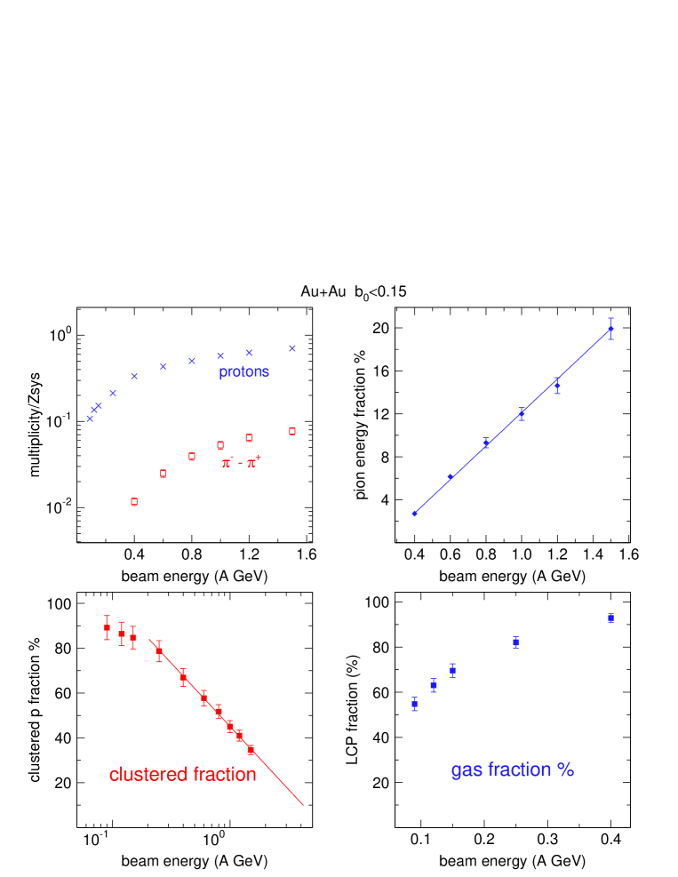
Figure 41: Some global characteristics of central Au+Au collisions as function of incident energy. Upper left panel: Reduced proton multiplicities and charge conversions by pion emission. Upper right panel: fraction (in $\%$) of total energy emitted as pions. Lower left panel: $\%$ fraction of protons in clusters. Lower right panel: measured nuclear charge fraction (in $\%$) emitted as LCP.

Even without a detailed comparison with statistical or dynamical codes a number of interesting features can be deduced by just plotting some of the information enclosed in our chemistry data. We begin with some global features, shown in Fig. 41. As illustrated in the upper left panel, in the SIS energy range the percentage of single protons emitted in central Au+Au collisions starts at the lower end at roughly the $10\%$ level to gradually increase to about $2/3$ of the available charge at $1.5A$ GeV.

The fraction complementary to single protons, the clustered fraction, is plotted separately again in the lower left panel. Although it contains no additional information, since it must complement the proton fraction to $100\%$, the ordinate is now linear and the abscissa is now logarithmic, allowing, in this representation, to illustrate a linear trend above $0.2A$ GeV (see the straight line, that reproduces the data with an accuracy of $1.5\%$) that suggests by extrapolation that the clustered fraction stays above $10\%$ all the way up to $4A$ GeV. This persistence of a significant probability to clusterize at freeze-out up to an available energy per nucleon more than two orders of magnitude higher than typical nucleonic binding energies is a remarkable signal of the local cooling process accompanying the fireball expansion and serves as a strong constraint on the associated entropy.

In some of the literature, see for example [75], particles with $Z\leq 2$ (LCP’s) are supposed to be the ingredients of nuclear matter in the gas state. These are the particles most easily evaporated from a hot liquid and therefore forming the gaseous atmosphere above the liquid. If one accepts this simple view then the ’fifty-fifty’ crossing liquid-gas takes place around $80A$ MeV beam energy. Since ’gas’ and ’liquid’ should add up to $100\%$, one can also read off the ’liquid’ fraction from the figure, which we call heavy clusters (or ’droplets’ [34]) and which is called frequently IMF (intermediate mass fragments) in the literature. Above $0.4A$ GeV the liquid fraction is $5\%$ or less. In the energy range considered here, fully central collisions do not lead any longer to fission-like (slightly less than half the projectile or target mass) or compound-nuclear-like (half or more than the total mass) remnants.

The SIS energy regime is also the regime where particle creation, very dominantly pions, varies from a ’perturbative’ low level to a significant fraction expected to heavily influence the global dynamics. Thus, the energy fraction rises to the $20\%$ level as seen in the upper right panel. The pertinent data were obtained from [38].

The non-perturbative nature of pions at the high end of this energy regime is also active for the isospin degree of freedom. According to the difference in $\pi^{-}$ and $\pi^{+}$ production, [38], plotted also in the upper left panel, some eight protons are converted to neutrons at freeze out, modifying substantially the initial $N/Z$ (from 1.494 to 1.264), a feature that in turn will modify the relative yields of the isotopes of hydrogen and helium.

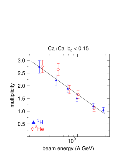
Figure 42: ³He and ${}^{3}H$ multiplicities in central ⁴⁰Ca+⁴⁰Ca collisions as function of the incident beam energy. The straight line is a common fit linearly decreasing with the logarithm of the energy.

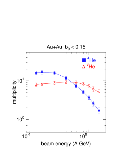
Figure 43: ³He and ${}^{4}He$ multiplicities in central Au+Au collisions as function of the incident beam energy. The ’crossing’ energy is $0.5A$ GeV.

We will later compare yields of the isospin pair ³He and ³H. It is therefore of some interest to check if the yields are equal in an isospin symmetric system such as ⁴⁰Ca+⁴⁰Ca. In this system only Coulomb effects could be invoked to predict different yields for the two isobaric clusters. Within experimental uncertainties the yields are equal in the investigated energy range (0.4 to $2A$ GeV), see Fig. 43.

We have already discussed in section 5 the non-perturbative character of clusterization. The high degree of clusterization seen in Fig. 41 confirms this aspect. In Fig. 43 we show excitation functions for the two He isotopes in central collisions of Au+Au. The two functions cross around 0.5A GeV. Clearly a simple perturbative coalescence model [43] could not explain this behaviour.

8.1 Mid-rapidity chemistry

In the present energy range a clean separation between ’participating’ (originally overlapping) matter and (peripheral) ’spectator’ matter is not possible as, especially in the most central collisions, there are no readily identifiable ’spectators’ moving undisturbed into angles close to the beam direction. Rather there is a superposition of various ejectiles having a more or less violent collision history as suggested by the observed stopping hierarchies (section 6). To minimize the effects of less violent and less equilibrated surface collisions, we concentrate our attention to (longitudinal) ’midrapidity chemistry’, defined here by a cut $|y_{z0}|<0.5$. As explained already in section 5, we remove some of the arbitrariness of the $|y_{z0}|$ cut using the thermal model fits to the constrained rapidity distributions applying the same cut and then correcting for the cut-out part using the fitted model data. This gives us an estimate of mid-rapidity yields extended to full rapidity.

In order to remove trivial size dependences we present ratios to proton yields, loosely writing e.g. d/p for the ratio of deuterons to protons. We shall see that even these ’size-reduced’ observables (and hence the extracted effective thermal parameters) are definitely still system size dependent. Furthermore, using the isospin pairs ³H/³He and $\pi^{-}$/$\pi^{+}$, we are able to separate size and isospin dependences: like the study of ground state masses, also the variation of the reaction systems along the valley of stability to change the system size necessarily leads to strongly correlated simultaneous change of the isospin of the system. For $0.15A$, $0.4A$, $1.0A$ and $1.5A$ GeV we show the results of this kind of analysis, see the next four figures, Figs. 44 to 47, and their captions. To each of these figures we add a panel showing the characteristics of the studied systems in terms of $N/Z$ versus $A_{sys}$. To better see the system size variations relative to the lightest system (Ni+Ni at the lowest energy, Ca+Ca at the higher energies), we also use double ratios. As a main conclusion from these rich data we can say that there is a significant influence of both system size and system composition on the outcoming yields of light clusters and of pions. When averaging over the isospin partners ³He/³H, resp. $\pi^{-}/\pi^{+}$ we see (left lower panels in Figs. 45 to 47) a regular evolution of the system-size dependence with the mass of the ejectile. In particular we confirm the weak dependence of total, or isospin averaged, pion multiplicities [38].

In contrast, in the upper two panels of the same figures the data for two isospin partners are seen to branch off as the $N/Z$ is varied along with the size. In an isospin asymmetric $(N>Z)$ medium like ¹⁹⁷Au + ¹⁹⁷Au (in contrast to ⁴⁰Ca + ⁴⁰Ca, Fig. 43) more n-n than p-p collisions take place, hence more $\pi^{-}$ than $\pi^{+}$ are produced (see also our work ref. [38]). For similar combinatorics reasons more ³H than ³He are synthesized. The more interesting question is whether this is also influenced by density-dependent long-range isovector potentials. This question, so far, is not settled. For instance, for pion ratios, see the contradictig references [76, 77, 78]. Concerning ³He and ³H, to our knowledge no microscopic transport code has reproduced so far the special ’anomaly’ features discussed earlier in connection with Figs. 17 and 18 in section 5.2 and Fig. 29 (right panel) in section 7. This makes also a convincing rendering of the experimental yield data difficult. Obviously more work is necessary.

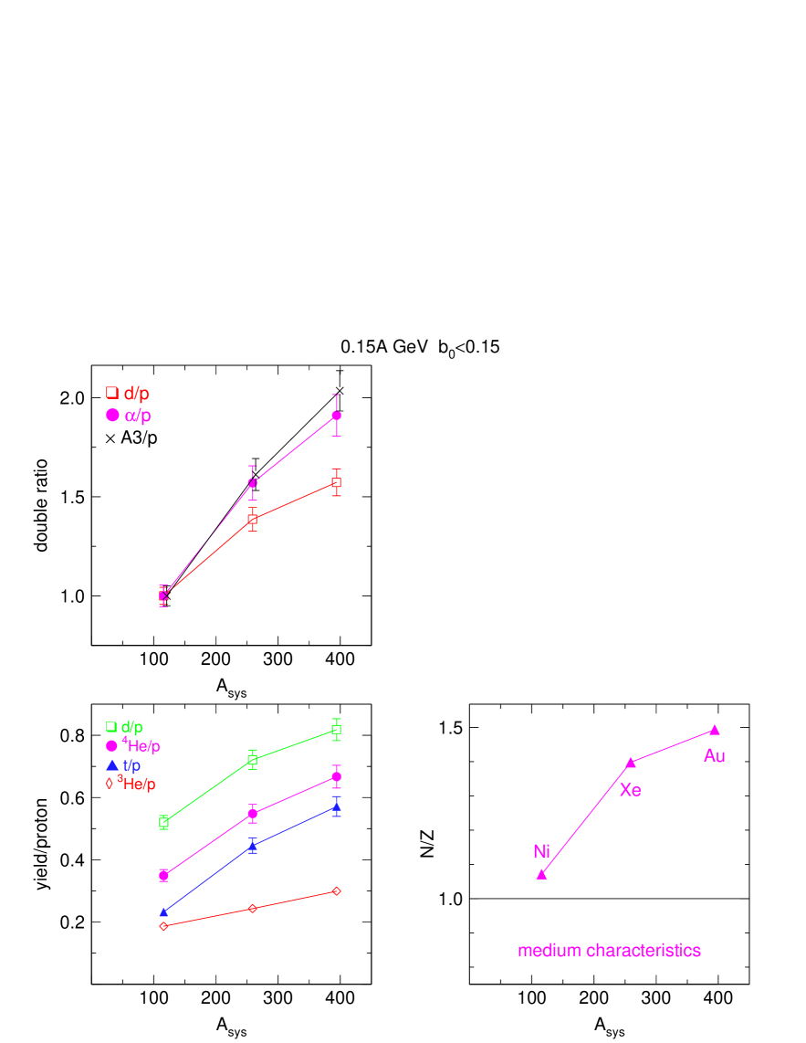
Figure 44: System size dependences for beam energies of $0.15A$ GeV. Lower left panel: yield ratios relative to protons for ⁴He (pink closed circles), ³He (red open diamonds), tritons (blue closed triangles) and deuterons (green open squares). Upper left panel: system size dependence of mass two, three and four yields relative to protons. The plotted double ratios are relative to the corresponding ratio in the Ni+Ni system $(A_{sys}=116)$. The medium characteristics for the three studied systems in terms of $N/Z$ and total mass $A_{sys}$ are drawn in the lower right panel.

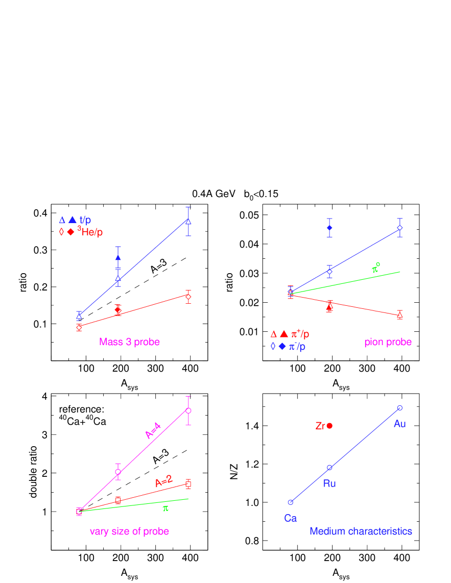
Figure 45: System size dependences for beam energies of $0.4A$ GeV. Upper left panel: $t/p$ and ³He/p ratio, upper right panel: $\pi^{+}/p$ and $\pi^{-}/p$. The straight lines are linear fits excluding the Zr+Zr data points which are plotted with full symbols. The resulting (linear) ’isospin averaged’ trends are also drawn. Lower left panel: double ratios (with respect to protons and relative to the Ca+Ca system, $A_{sys}=80$) for mass 4, 3, 2 fragments and pions (upper to lower curves). The Zr+Zr data points are not included here. The medium characteristics for the four studied systems in terms of $N/Z$ and total mass $A_{sys}$ are drawn in the lower right panel.

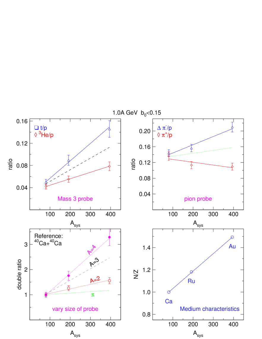
Figure 46: System size dependences for beam energies of $1.0A$ GeV. Upper left panel: $t/p$ and ³He/p ratio, upper right panel: $\pi^{+}/p$ and $\pi^{-}/p$. The straight lines are linear fits guiding the eye. The resulting (linear) ’isospin averaged’ trends are also drawn. Lower left panel: double ratios (with respect to protons and relative to the Ca+Ca system, $A_{sys}=80$) for mass 4, 3, 2 fragments and pions (upper to lower curves). The medium characteristics for the three studied systems in terms of $N/Z$ and total mass $A_{sys}$ are drawn in the lower right panel.

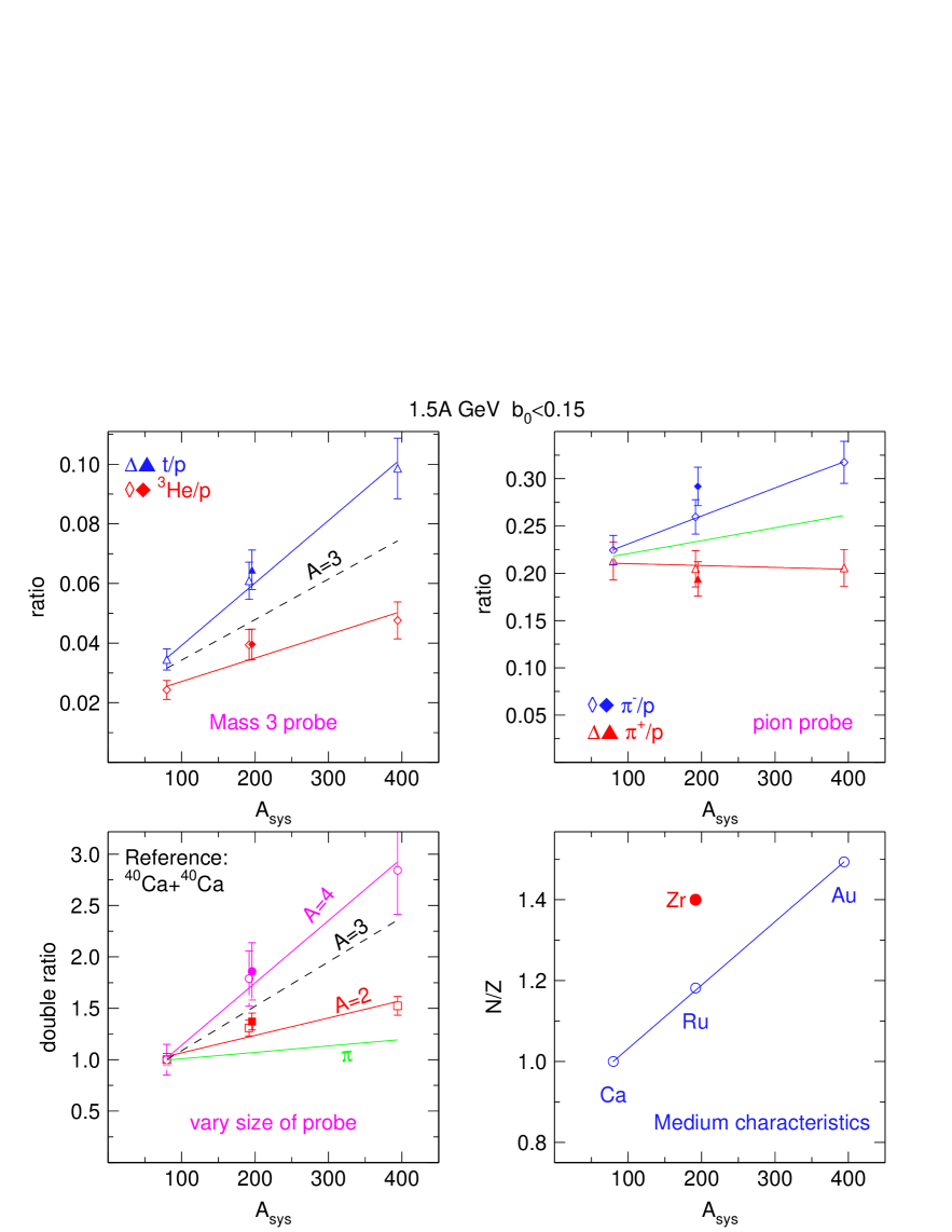
Figure 47: System size dependences for beam energies of $1.5A$ GeV. Upper left panel: $t/p$ and ³He/p ratio, upper right panel: $\pi^{+}/p$ and $\pi^{-}/p$. The straight lines are linear fits guiding the eye. The resulting (linear) ’isospin averaged’ trends are also drawn. Lower left panel: double ratios (with respect to protons and relative to the Ca+Ca system, $A_{sys}=80$) for mass 4, 3, 2 fragments and pions (upper to lower curves). Data for the Zr+Zr system are drawn as full symbols and are not included in the fits. The medium characteristics for the four studied systems in terms of $N/Z$ and total mass $A_{sys}$ are drawn in the lower right panel.

A final important point to make on the chemistry is the strong correlation of the yields, the transverse rapidity variances and the fragment specific stopping when varying the system sizes $Z_{sys}$. This effect is best illustrated when feeding from higher mass clusters is small so that one can envision the synthesis of new nuclei from a hot expanding, originally nucleonic, soup. In view of the steep decrease of yields with fragment size, this condition could be safely assumed to be fulfilled at $0.4A$ GeV for Li [34]. As is shown in Fig. 48 the same can be assumed to be true at $1.0A$ GeV for ⁴He clusters and at $1.5A$ GeV for mass three clusters. To remove superimposed isospin effects we have added the mass three H and He isotopes. Increased stopping (right panels) indicates increased compression. The increasing constrained transverse rapidity variances varxm0 (middle panels) are interpreted as increasing radial flow developed thereafter in the expansion phase which is coupled to increased cooling (’droplet formation’). (We remind the reader that not only the variances, but also the shapes of these distributions were well described by a thermal shape assuming an equivalent temperature $T_{eq}$, see section 5.1 and figs. 11-16.) The interpretation is supported by the remarkable, close-to-quadratic (the power is $1.7\pm 0.1$) system-size dependences of the mid-rapidity cluster multiplicities already stressed in ref. [34]. Kaon ($K^{+}$) production in the SIS energy range is also known [19] to show stronger than linear size dependences associated to varying achieved compressions. The mechanisms are different however: in the kaon case there is increased production in the high density case which thereafter, in contrast to pion production , is partially ’memorized’ due to small $K^{+}$ reaction cross sections making the cooling phase ’inefficient’. For clusters we start ’from zero’ at maximum achieved density, but increased compression leading to subsequent increased cooling creates more clusters. In this sense we suggest that this process, like $K^{+}$ production, is sensitive to the EOS because it partially memorizes the initial compression which, in turn, is largest for softest EOS.

Loosely speaking, we are thus witnessing the creation of nuclei in a mini-’supernova’. With increasing beam energy we catch earlier, hotter, stages forming smaller nuclei. For a theoretical treatment of the $0.4A$ GeV data in this connection see [61]. This work supports our interpretation and shows that understanding this ’fast’ synthesis of nuclei is not outside our present theoretical capabilities, although there is room for improvement.

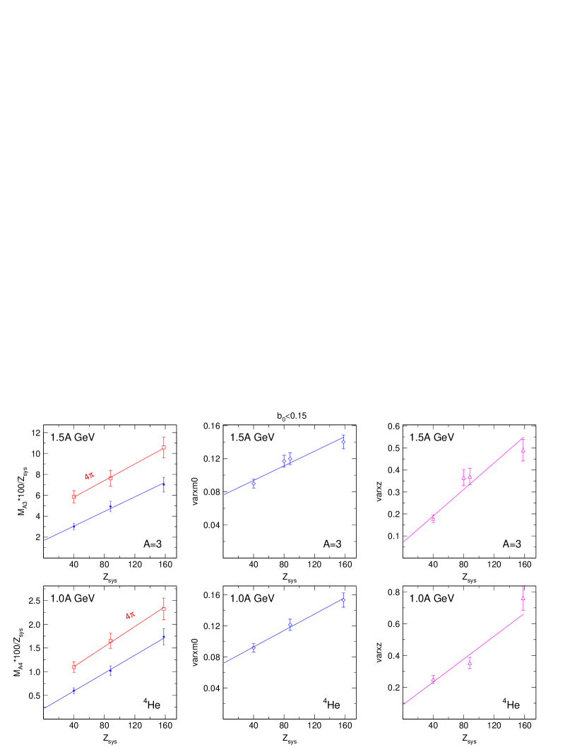
Figure 48: System size dependences of symmetric central collisions at incident beam energies of $1.0A$ GeV (lower panels, ⁴He fragments) and $1.5A$ GeV (upper panels, average of ³He and ³H fragments). All straight lines are linear fits. Left panels: Multiplicities (reduced to 100 protons). The data marked $4\pi$ with open square symbols are $4\pi$ integrated, while the closed symbols represent mid-rapidity yields (constrained to $|y_{z0}|<0.5$). Middle panels: Variance varxm0 of the scaled constrained transverse rapidity distributions ($dn/dy_{xm0}$). Right panels: stopping varxz.

9 Summary

We summarize here the results presented in sections 5 to 8. In a study involving 25 system-energies we have been able to establish a vast systematics of very central heavy ion collisions in the SIS energy range. We started characterizing the data for identified ejectiles by rapidity distributions both in the longitudinal and the transverse directions relative to the beam axis. As a very general rule we found that the variance of the longitudinal distribution was always broader than the variance of the transverse direction. This effect was most pronounced at the highest incident energy (Figs. 11, 12).

We also introduced a transverse distribution constrained by a cut $|y_{z0}|<0.5$ on the scaled longitudinal rapidity (the definitions were given in section 3) and found that its shape, plotted on a linear scale, could always be very well described by a thermal distribution defining thus an equivalent ’temperature’ $T_{eq}$ that was characteristic for each particle, incident energy and centrality. This equivalent temperature was found in general to rise with the particle’s mass, Fig. 13, an effect that could be qualitatively reproduced by IQMD simulations, Fig. 14, although the shapes of the simulated distributions looked less perfectly thermal and the $T_{eq}$ followed the experimental data only approximately.

At $1.5A$ GeV beam energy the rise of $T_{eq}$ with mass could also be followed with the He isotopes and as a consequence of this behaviour it could be shown that the spectra of heavier particles could not simply be derived by power law from the proton spectra, Fig. 15 somewhat in contradiction to messages published in ref. [43].

The $T_{eq}$ were shown to rise significantly with centrality, Fig. 16. At lower incident energies a remarkable deviation of the mass trend of $T_{eq}$ was observed: the ⁴He value tended to be lower than the ³He value. This ’He anomaly’ [44] and large differences between ³H and ${}^{3}He$ spectra were tentatively associated with clusterization phenomena, Figs. 17, 18, illustrating the fact that a proper rendering of cluster probabilities was essential if simulations were to be used for extracting basic information from the data.

The systematic comparison of transverse and longitudinal rapidity distributions, Fig. 19, turned out to be a rich source of information, as one observes remarkable variations with incident energy and system size. Although the shapes of the distributions showed features that cannot be fully described by one parameter, we proposed to summarize the differential information by a stopping observable varxz, the ratio of variances of transverse to longitudinal rapidity distributions. Stopping was always found to have values below one, a fact that we interpreted as partial transparency or incomplete stopping on account of the system size dependences. The hydrodynamic rebound expected in the full stopping scenario could also be definitely excluded by use of isospin tracer methods introduced earlier [52] by our Collaboration: an increase of transparency at the high end of the studied energy range, Fig. 20, could be unambiguously confirmed.

We were able to confront the global stopping observable [32] with simulations varying the stiffness of the nuclear EOS. The most striking feature of the excitation function for the Au+Au system, namely the existence of a pronounced maximum for $E/A=0.2A$ to $0.8A$ GeV could be qualitatively reproduced, but the strong descent at higher energies to decreased stopping was underestimated, Fig. 21. The predictions for varxz were found to be sufficiently sensitive to the EOS to exceed the experimental uncertainty: this adds another constraint from central collisions to efforts to fix the EOS from heavy ion data.

Moving beyond global observables to individual stopping data associated to specific identified particles, we found stopping to be essentially a collective phenomenon, Fig. 22, but a closer inspection also established that there was a hierarchy of stopping suggesting that heavier clusters were in part connected on the average with a less violent collision history. This hierarchy was weakest in the maximum of the stopping excitation function, Fig. 23, but otherwise followed as a function of isotope mass, incident energy and system size a rather complex behaviour reflecting the rich data presented earlier in Fig. 19 and representing a challenge to future simulations, Fig. 24. Surprisingly, we could not find a significant dependence of stopping on isospin at $0.4A$ and $1.5A$ GeV, Fig. 25, while the expected strong dependence on centrality, Fig. 26, is a warning that centrality must be well matched to experiment when simulations are done.

For the lower energies we have confirmed that the stopping hierarchy is omnipresent also for all heavier clusters up to $Z=8$. In an attempt to join up to energies higher than were studied here we showed the strong trend for increasing transparency of leading protons as the energy is raised to AGS and SPS energies.

Passing from the compression stage, characterized by the stopping observable, we studied the expansion stage, characterized by radial flow, which is generally inferred by mass dependences of kinetic energies or equivalent temperatures. We found that average kinetic energies of identified particles emitted at $90^{\circ}$ follow extremely regular patterns as a function of incident energy, Fig. 29, the details of which, like the ³H-³He difference, can only be understood if the simulation predicts clusterization correctly, Figs. 30, 31. If we combine the data for protons, deuterons and the average of the two mass three isotopes (’A3 method’), we can establish a radial flow systematics for Au+Au extending from $0.09A$ to $1.5A$ GeV which is in fair agreement in the overlapping energy range with [45]. We find a strong system size dependence of radial flow, Fig. 33, which is however not reproduced quantitatively by IQMD simulations, Fig. 34. In agreement with [45] we find that the mass dependences of kinetic energies are strongly dependent on the emission angles, Fig. 35, leading to a necessary reassessment of the origin of the ’flow’ deduced in our earlier work on heavy clusters [40]. In general the observed partial transparencies and stopping hierarchies call for a more qualified interpretation of the data, as illustrated in Fig. 36.

Using the equivalent temperatures, based on constrained transverse rapidity distributions, we observe the same structural characteristics if we plot $T_{eq}$ versus mass for the five LCP, Fig. 37. The system size evolution of $T_{eq}$ is quite different for nucleonic clusters than for pions, Fig. 38 reflecting the different mechanisms of creation/annihilation. The presence of ’spectator’ matter in non-central collisions influences the resulting $T_{eq}$, Fig. 39.

A systematics of $T_{eq}$ for all five LCP versus impact parameter is presented in Fig. 40 and allows to extrapolate to $b_{0}=0$.

The final state of the system after expansion-cooling is described by its chemical composition which we have tabulated in the appendix for the twenty-five system energies. For energies below $0.2A$ GeV we are consistent with INDRA-ALADIN data [33, 64, 65], while quite satisfactory agreement with the pioneering PLASTIC BALL experiments [67] could be demonstrated, see Table 1, for cases of overlap. Throughout the SIS-BEVALAC energy range clusterization is an important feature, Fig. 41, that cannot be treated by perturbative coalescence models and influences significantly the spectra and flow of all particles: hence conclusions from the data with the help of transport codes must handle correctly this aspect of the reactions. At the same time, particle creation (pions) in this energy range rises gradually from a perturbative level to as much as $20\%$ in terms of the energy fraction at $1.5A$ GeV (many more details, connected with pions and obtained with the FOPI setup, were published in [38]). At the lower energy end $\alpha$ particles play a special role: below $0.5A$ GeV more $\alpha$ particles are emitted than ³He ejectiles, Fig. 43, and $\alpha$ particle condensation is probably needed to explain in detail the very different ³He and ³H spectra as suggested by our discussion of Figs.17 and 18. There is a notable system-size and isospin dependence of the chemical ’temperatures’ that we evidenced using isospin pairs like ³He-³H and $\pi^{+}$-$\pi^{-}$ in various systems, Figs. 44-47.

Finally, our yield data suggest that there is at least a partial memory of the initial degree of compression, and hence the stiffness of the EOS: more compression leads to more efficient subsequent cooling enhancing the degree of clusterization. This is suggested by the close to quadratic dependence on system size and the conspicuous correlations between cluster yields, radial flow and stopping evidenced in the last figure of this paper and in [34].

Appendix: Yield tables

Multiplicities and charge balance for Au+Au at $E/A=0.09$ GeV and $b_{0}<0.15$.

Z=1	$40.1\pm 2.1$	p	$17.0\pm 0.9$	Z=2	$23.2\pm 1.7$	3He
		d	$13.3\pm 1.0$			4He
		t	$9.7\pm 1.0$

Li	$4.1\pm 0.4$	Be	$1.77\pm 0.18$
B	$1.79\pm 0.18$	C	$1.43\pm 0.15$

Charge balance LCP: 86.5 or $54.8\%$
Charge in HC Z3-Z6 (measured): $36.8\pm 3.7$ or $(23.3\pm 2.4)\%$
Charge measured: 123.3 or $78.0\%$
Charge in HC: 158-86.5=71.5 or $45.3\%$

Multiplicities and charge balance for Au+Au at $E/A=0.12$ GeV and $b_{0}<0.15$.

Z=1	$51.5\pm 2.6$	p	$21.5\pm 1.1$	Z=2	$24.2\pm 1.7$	3He	$8.0\pm 0.8$
		d	$17.6\pm 1.2$			4He	$16.2\pm 1.6$
		t	$12.2\pm 1.2$

Li	$4.7\pm 0.5$	Be	$1.75\pm 0.18$
B	$1.62\pm 0.16$	C	$1.16\pm 0.12$
N	$0.71\pm 0.07$	O	$0.37\pm 0.04$

Charge balance LCP: 99.7 or $63.1\%$
Charge in HC Z3-Z8 (measured): $43.9\pm 4.4$ or $(27.8\pm 2.8)\%$
Charge measured: 143.6 or $90.9\%$
Charge in HC Z9-Z14 (estimated): $8.2\pm 3.0$ or $(5.2\pm 1.9)\%$
Total balance: $96.1\%$
Adopted IMF charge: $55.2\pm 5$ or $34.9\%$

Multiplicities and charge balance for Ni+Ni at $E/A=0.15$ GeV and $b_{0}<0.15$.

Z=1	$27.3\pm 1.4$	p	$15.1\pm 0.8$	Z=2	$10.8\pm 0.8$	3He	$4.06\pm 0.41$
		d	$8.4\pm 0.6$			4He	$6.71\pm 0.68$
		t	$3.74\pm 0.4$

Li	$1.24\pm 0.13$	Be	$0.42\pm 0.04$
B	$0.25\pm 0.03$	C	$0.18\pm 0.02$

Charge balance LCP: 48.84 or $87.2\%$
Charge in HC: 7.69 or $(13.7\pm 1.4)\%$
Total balance: 56.53 or $100.9\%$

Multiplicities and charge balance for Xe+CsI at $E/A=0.15$ GeV and $b_{0}<0.15$.

Z=1	$46.0\pm 2.3$	p	$20.1\pm 1.0$	Z=2	$18.8\pm 1.3$	3He	$5.9\pm 0.6$
		d	$15.6\pm 1.1$			4He	$12.9\pm 1.3$
		t	$10.3\pm 1.0$

Li	$2.77\pm 0.28$	Be	$0.89\pm 0.09$
B	$0.67\pm 0.07$	C	$0.41\pm 0.04$
N	$0.19\pm 0.02$	O	$0.10\pm 0.01$

Charge balance LCP: 83.53 or $77.3\%$
Charge in HC: 19.83 or $(18.4\pm 1.8)\%$
Total balance: 103.36 or $95.7\%$

Multiplicities and charge balance for Au+Au at $E/A=0.15$ GeV and $b_{0}<0.15$.

Z=1	$59.9\pm 3.0$	p	$24.1\pm 1.2$	Z=2	$25.0\pm 1.8$	3He	$8.4\pm 0.9$
		d	$20.4\pm 1.4$			4He	$16.6\pm 1.7$
		t	$15.1\pm 1.5$

Li	$5.0\pm 0.5$	Be	$1.69\pm 0.17$
B	$1.44\pm 0.15$	C	$0.90\pm 0.09$
N	$0.50\pm 0.05$	O	$0.26\pm 0.03$

Charge balance LCP: 109.9 or $69.6\%$
Charge in HC Z3-Z8 (measured): $40.0\pm 4$ or $(25.3\pm 2.5)\%$
Charge measured: 149.9 or $94.9\%$
Charge in HC Z9-Z14 (estimated): $4.4\pm 1.5$ or $(2.8\pm 1)\%$
Total balance: $97.7\%$

Multiplicities and charge balance for Ni+Ni at $E/A=0.25$ GeV and $b_{0}<0.15$.

Z=1	$34.9\pm 1.8$	p	$19.2\pm 1.0$	Z=2	$9.0\pm 0.7$	3He	$3.24\pm 0.33$
		d	$10.5\pm 0.8$			4He	$5.79\pm 0.58$
		t	$5.1\pm 0.5$

Li	$0.91\pm 0.09$	Be	$0.26\pm 0.03$
B	$0.10\pm 0.01$

Charge balance LCP: 52.93 or $94.5\%$
Charge in HC: 4.28 or $(7.6\pm 0.8)\%$
Total balance: 57.21 or $102.2\%$

Multiplicities and charge balance for Xe+CsI at $E/A=0.25$ GeV and $b_{0}<0.15$.

Z=1	$59.6\pm 3.0$	p	$26.3\pm 1.4$	Z=2	$16.7\pm 1.2$	3He	$6.0\pm 0.6$
		d	$19.3\pm 1.4$			4He	$10.8\pm 1.1$
		t	$14.1\pm 1.5$

Li	$2.33\pm 0.23$	Be	$0.60\pm 0.06$
B	$0.29\pm 0.03$	C	$0.14\pm 0.02$
N	$0.05\pm 0.01$

Charge balance LCP: 92.99 or $86.1\%$
Charge in HC: 12.65 or $(11.7\pm 1.2)\%$
Total balance: 105.64 or $97.8\%$

Multiplicities and charge balance for Au+Au at $E/A=0.25$ GeV and $b_{0}<0.15$.

Z=1	$79.9\pm 4.0$	p	$33.7\pm 1.7$	Z=2	$24.8\pm 1.7$	3He	$8.8\pm 0.9$
		d	$26.7\pm 1.9$			4He	$16.0\pm 1.6$
		t	$19.5\pm 2.0$

Li	$4.5\pm 0.4$	Be	$1.32\pm 0.13$
B	$0.67\pm 0.07$	C	$0.35\pm 0.04$
N	$0.13\pm 0.02$

Charge balance LCP: $82.1\%$
Charge in HC: 26.0 or $(16.45\pm 1.7)\%$
measured HC charge (Z3-Z7): 25.08, estim (Z8-Z10): 0.91
Total balance: $98.5\%$

Multiplicities and charge balance for Au+Au at $E/A=0.40$ GeV and $b_{0}<0.15$.

Z=1	$106.0\pm 4.0$	p	$52.9\pm 2.7$	Z=2	$21.3\pm 1.9$	3He	$9.4\pm 0.9$
		d	$34.2\pm 2.1$			4He	$11.9\pm 1.1$
		t	$19.4\pm 1.8$
$\pi^{+}$	$0.95\pm 0.08$	$\pi^{-}$	$2.80\pm 0.14$

Li	$3.5\pm 0.4$	Be	$0.84\pm 0.09$
B	$0.27\pm 0.03$	C	$0.096\pm 0.01$

Charge balance LCP: 148.6 or $94.1\%$
Charge balance LCP+pions: 146.8 or $92.9\%$
Charge in HC (Z3-Z6): $15.77\pm 1.6$ or $(10.0\pm 1.0)\%$
Total balance: $102.9\%$

Multiplicities and charge balance for Au+Au at $E/A=0.6$ GeV and $b_{0}<0.15$. Z=1 $121.9\pm 6.1$ p $68.5\pm 3.5$ Z=2 $16.4\pm 1.5$ ³He $9.1\pm 0.9$ d $36.6\pm 2.2$ ⁴He $7.4\pm 0.7$ t $16.8\pm 1.5$ $\pi^{+}$ $3.14\pm 0.25$ $\pi^{-}$ $7.08\pm 0.36$

Charge balance LCP+pions: $95.4\%$
Estimate IMF: $(6\pm 2)\%$
Total balance: $101.4\%$

Multiplicities and charge balance for Au+Au at $E/A=0.8$ GeV and $b_{0}<0.15$. Z=1 $132.51\pm 6.6$ p $79.4\pm 4.0$ Z=2 $13.5\pm 1.2$ ³He $8.2\pm 0.8$ d $37.7\pm 2.3$ ⁴He $5.2\pm 0.5$ t $15.4\pm 1.6$ $\pi^{+}$ $6.26\pm 0.50$ $\pi^{-}$ $12.49\pm 0.63$

Charge balance LCP+pions: 153.3 or $97.0\%$
Estimate IMF: $(4\pm 2)\%$
Total balance: $101.0\%$

Multiplicities and charge balance for Au+Au at $E/A=1.0$ GeV and $b_{0}<0.15$. Z=1 $140.9\pm 7.0$ p $91.5\pm 4.0$ Z=2 $11.0\pm 1.2$ ³He $7.3\pm 0.7$ d $38.8\pm 2.3$ ⁴He $3.7\pm 0.4$ t $13.9\pm 1.3$ $\pi^{+}$ $9.87\pm 0.79$ $\pi^{-}$ $18.26\pm 0.91$

Charge balance LCP+pions: 154.5 or $97.8\%$
IMF order $2\%$ ($<4\%$)
Total balance: $99.8\%$

Multiplicities and charge balance for Au+Au at $E/A=1.2$ GeV and $b_{0}<0.15$. Z=1 $148.2\pm 7.0$ p $99.3\pm 4.0$ Z=2 $8.74\pm 1.3$ ³He $6.1\pm 0.9$ d $36.8\pm 2.3$ ⁴He $2.6\pm 0.4$ t $12.1\pm 1.3$ $\pi^{+}$ $14.13\pm 1.13$ $\pi^{-}$ $24.37\pm 1.22$

Charge balance LCP+pions: 155.5 or $98.4\%$
IMF neglected
Total balance: $98.4\%$ (IMF neglected)

Multiplicities and charge balance for Au+Au at $E/A=1.5$ GeV and $b_{0}<0.15$. Z=1 $158.4\pm 7.0$ p $111.3\pm 5.6$ Z=2 $6.76\pm 1.3$ ³He $5.1\pm 0.8$ d $36.0\pm 2.2$ ⁴He $1.7\pm 0.3$ t $11.0\pm 1.1$ $\pi^{+}$ $21.16\pm 1.70$ $\pi^{-}$ $33.34\pm 1.67$

Charge balance LCP+pions: 159.7 or $101.1\%$
IMF neglected
Total balance: $101.3\%$ (IMF neglected)

Multiplicities and charge balance for Ru+Ru at $E/A=0.4$ GeV and $b_{0}<0.15$. Z=1 $59.8\pm 3.0$ p $33.2\pm 1.7$ Z=2 $11.0\pm 1.0$ ³He $5.6\pm 0.5$ d $18.3\pm 1.1$ ⁴He $5.4\pm 0.5$ t $8.3\pm 0.8$ $\pi^{+}$ $0.70\pm 0.06$ $\pi^{-}$ $1.07\pm 0.06$ Li $1.28\pm 0.13$ Be $0.28\pm 0.03$

Charge balance LCP+pions: 81.37 or $92.5\%$
Total charge IMF : 5.5 or $6.2\%$ (estimate 0.5 for $Z>4$)
Total balance: $92.5+6.2=98.7\%$

Multiplicities and charge balance for Zr+Zr at $E/A=0.4$ GeV and $b_{0}<0.15$. Z=1 $56.0\pm 2.8$ p $28.8\pm 1.5$ Z=2 $10.2\pm 1.0$ ³He $4.8\pm 0.4$ d $18.3\pm 1.1$ ⁴He $5.4\pm 0.5$ t $8.9\pm 0.8$ $\pi^{+}$ $0.56\pm 0.05$ $\pi^{-}$ $1.42\pm 0.07$ Li $1.22\pm 0.13$ Be $0.29\pm 0.03$

Charge balance LCP+pions: 75.49 or $94.4\%$
Total charge IMF : 5.3 or $6.6\%$ (estimate 0.5 for $Z>4$)
Total balance: $94.4+6.6=101.0\%$

Multiplicities and charge balance for Ru+Ru at $E/A=1.0$ GeV and $b_{0}<0.15$. Z=1 $79.1\pm 4.0$ p $53.9\pm 2.7$ Z=2 $5.17\pm 0.47$ ³He $3.68\pm 0.33$ d $19.7\pm 1.2$ ⁴He $1.49\pm 0.14$ t $5.5\pm 0.5$ $\pi^{+}$ $6.05\pm 0.49$ $\pi^{-}$ $8.09\pm 0.41$

Charge balance LCP+pions: 87.38 or $99.3\%$
IMF neglected

Multiplicities and charge balance for Ru+Ru at $E/A=1.5$ GeV and $b_{0}<0.15$. Z=1 $87.03\pm 4.4$ p $64.5\pm 3.2$ Z=2 $3.32\pm 0.3$ ³He $2.65\pm 0.24$ d $18.4\pm 1.1$ ⁴He $0.67\pm 0.06$ t $4.1\pm 0.4$ $\pi^{+}$ $12.49\pm 1.00$ $\pi^{-}$ $15.63\pm 0.78$

Charge balance LCP+pions: 90.52 or $102.9\%$
IMF neglected

Multiplicities and charge balance for Zr+Zr at $E/A=1.5$ GeV and $b_{0}<0.15$. Z=1 $84.3\pm 4.2$ p $61.3\pm 3.1$ Z=2 $3.26\pm 0.32$ ³He $2.61\pm 0.24$ d $18.6\pm 1.1$ ⁴He $0.65\pm 0.06$ t $4.3\pm 0.4$ $\pi^{+}$ $11.45\pm 0.92$ $\pi^{-}$ $17.19\pm 0.86$

Charge balance LCP+pions: 85.09 or $106.4\%$
IMF neglected

Multiplicities and charge balance for Ca+Ca at $E/A=0.4$ GeV and $b_{0}<0.15$. Z=1 $30.5\pm 1.6$ p $19.1\pm 1.0$ Z=2 $4.9\pm 0.5$ ³He $2.8\pm 0.3$ d $8.6\pm 0.5$ ⁴He $2.1\pm 0.2$ t $2.7\pm 0.3$ $\pi^{+}$ $0.45\pm 0.04$ $\pi^{-}$ $0.47\pm 0.03$

Charge balance LCP+pions: 40.29 or $100.7\%$
Z3 $0.34\pm 0.04$
Charge balance: 40.29+1.02=41.31 or $103.3\%$

Multiplicities and charge balance for Ca+Ca at $E/A=0.6$ GeV and $b_{0}<0.15$. Z=1 $33.2\pm 1.7$ p $22.9\pm 1.2$ Z=2 $3.7\pm 0.4$ ³He $2.6\pm 0.3$ d $8.1\pm 0.5$ ⁴He $1.1\pm 0.1$ t $2.2\pm 0.2$ $\pi^{+}$ $1.13\pm 0.09$ $\pi^{-}$ $1.28\pm 0.07$

Charge balance LCP+pions: 40.54 or $101.3\%$
IMF neglected

Multiplicities and charge balance for Ca+Ca at $E/A=0.8$ GeV and $b_{0}<0.15$. Z=1 $35.2\pm 1.8$ p $25.3\pm 1.3$ Z=2 $2.6\pm 0.2$ ³He $1.85\pm 0.23$ d $8.0\pm 0.5$ ⁴He $0.75\pm 0.09$ t $1.9\pm 0.2$ $\pi^{+}$ $2.11\pm 0.17$ $\pi^{-}$ $2.28\pm 0.11$

Charge balance LCP+pions: 40.24 or $100.6\%$

Multiplicities and charge balance for Ca+Ca at $E/A=1.0$ GeV and $b_{0}<0.15$. Z=1 $36.5\pm 1.8$ p $26.5\pm 1.4$ Z=2 $2.1\pm 0.2$ ³He $1.65\pm 0.15$ d $7.8\pm 0.5$ ⁴He $0.45\pm 0.04$ t $1.52\pm 0.14$ $\pi^{+}$ $3.16\pm 0.26$ $\pi^{-}$ $3.33\pm 0.17$

Charge balance LCP+pions: 40.57 or $101.4\%$

Multiplicities and charge balance for Ca+Ca at $E/A=1.5$ GeV and $b_{0}<0.15$. Z=1 $38.6\pm 1.8$ p $30.4\pm 1.6$ Z=2 $1.10\pm 0.16$ ³He $0.93\pm 0.16$ d $7.2\pm 0.5$ ⁴He $0.17\pm 0.03$ t $1.22\pm 0.15$ $\pi^{+}$ $5.62\pm 0.45$ $\pi^{-}$ $5.78\pm 0.30$

Charge balance LCP+pions: 40.64 or $101.6\%$

Multiplicities and charge balance for Ca+Ca at $E/A=1.93$ GeV and $b_{0}<0.15$. Z=1 $39.6\pm 1.8$ p $33.7\pm 1.7$ Z=2 $0.82\pm 0.20$ ³He $0.70\pm 0.14$ d $6.8\pm 0.5$ ⁴He $0.13\pm 0.03$ t $1.11\pm 0.15$ $\pi^{+}$ $7.82\pm 0.63$ $\pi^{-}$ $7.86\pm 0.40$

Charge balance LCP+pions: 41.22 or $103.1\%$

References

- [1] W. Scheid, et al., Phys. Rev. Lett. 32 (1974) 741; W. Schmidt, et al., Phys. Rev. C 47 (1993) 2782.
- [2] H. A. Gustafsson, et al., Phys. Rev. Lett. 52 (1984) 1590.
- [3] R. E. Renfordt, et al., Phys. Rev. Lett. 53 (1984) 763.
- [4] G. F. Bertsch, S. Das Gupta, Phys. Rep. 160 (1988) 189.
- [5] R. B. Clare, D. Strottman, Phys. Rep. 141 (1986) 177.
- [6] H. Stöcker, W. Greiner, Phys. Rep. 137 (1986) 277.
- [7] J. Aichelin, et al., Phys. Rev. Lett. 58 (1987) 1926.
- [8] C. Gale, et al., Phys. Rev. C 35 (1987) 1666.
- [9] G. E. Brown, M. Rho, Phys. Rev. Lett. 66 (1991) 2720.
- [10] C. Fuchs, A. Faessler, M. El-Shabshiry Phys. Rev. C 64 (2001) 024003.
- [11] P. Danielewicz, R. Lacey, W. G. Lynch, Science 298 (2002) 1592.
- [12] C. Fuchs, Prog. Part. Nucl. Phys. 56 (2006) 1.
- [13] C. Fuchs, H. H. Wolter, Eur. Phys. J. A30 (2006) 5.
- [14] W. Reisdorf, H. G. Ritter, Annu. Rev. Nucl. Part. Sci. 47 (1997) 663.
- [15] N. Herrmann, J. P. Wessels, T. Wienold, Annu. Rev. Nucl. Part. Sci. 49 (1999) 581.
- [16] C. Hartnack, H. Oeschler and J. Aichelin, Phys. Rev. Lett. 96 (2006) 012302.
- [17] C. Sturm et al. [KaoS Coll.], Phys. Rev. Lett. 86 (2001) 39.
- [18] P. Senger, H. Ströbele, J. Phys. G 25 (1999) R59.
- [19] A. Förster, et al. (KaoS Collaboration), Phys. Rev. C 75 (2007) 024906.
- [20] J. Aichelin, Che Ming Ko, Phys. Rev. Lett. 55 (1985) 2661.
- [21] V. Ramillien, et al. (FOPI Collaboration), Nucl. Phys. A 587 (1995) 802.
- [22] N. Bastid et al. (FOPI Collaboration), Nucl. Phys. A 622 (1997) 573.
- [23] P. Crochet, et al. (FOPI Collaboration), Nucl. Phys. A 627 (1997) 522, erratum Nucl. Phys. A 628 (1997) 687.
- [24] A. Andronic, et al. (FOPI Collaboration), Nucl. Phys. A 679 (2001) 765.
- [25] A. Andronic, et al. (FOPI Collaboration), Phys. Rev. C 64 (2001) 041604(R).
- [26] A. Andronic, et al. (FOPI Collaboration), Phys. Rev. C 67 (2003) 034907.
- [27] N. Bastid et al. (FOPI Collaboration), Nucl. Phys. A 742 (2004) 29.
- [28] G. Stoicea, et al. (FOPI Collaboration), Phys. Rev. Lett. 92 (2004) 072303.
- [29] A. Andronic, et al. (FOPI Collaboration), Phys. Lett. B 612 (2005) 173.
- [30] S. Wang, et al. (EOS Collaboration), Phys. Rev. Lett. 76 (1996) 3911.
- [31] H. Stöcker, M. Gyulassy, J. Boguta, Phys. Lett. B 103 (1981) 269.
- [32] W. Reisdorf, et al. (FOPI Collaboration), Phys. Rev. Lett. 92 (2004) 232301.
- [33] A. Andronic, J. Lukasik, W. Reisdorf, W. Trautmann, Eur. Phys. J. A30 (2006) 31.
- [34] W. Reisdorf, et al. (FOPI Collaboration), Phys. Lett. B 595 (2004) 118.
- [35] A. Gobbi, et al. (FOPI Collaboration), Nucl. Instr. Meth. A 324 (1993) 156.
- [36] J. Ritman, Nucl. Phys. B 44 (1995) 708.
- [37] C. Hartnack, et al., Eur. Phys. J. A 1 (1998) 151.
- [38] W. Reisdorf, et al. (FOPI Collaboration), Nucl. Phys. A 781 (2007) 457.
- [39] D. Pelte, et al. (FOPI Collaboration), Z. Phys. A 357 (1997) 215.
- [40] W. Reisdorf, et al. (FOPI Collaboration), Nucl. Phys. A 612 (1997) 493.
- [41] W. D. Myers, Nucl. Phys. A 204 (1973) 465; J. Błocki, J. Randrup, W. J. Swiatecki, C. F. Tsang, Ann. Phys. 105 (1977) 427.
- [42] G. Poggi, et al. (FOPI Collaboration), Nucl. Phys. A 586 (1995) 755.
- [43] S. Wang, et al. (EOS Collaboration), Phys. Rev. Lett. 74 (1995) 2646.
- [44] W. Neubert, A. S. Botvina, Eur. Phys. J. A 7 (2000) 101.
- [45] M.A. Lisa, et al. (EOS Collaboration), Phys. Rev. Lett. 75 (1995) 2662.
- [46] F. Videbaek and O. Hansen, Phys. Rev. C 52 (1995) 2684.
- [47] H. Ströbele, nucl-ex:0908.2777
- [48] B. Hong, et al. (FOPI Collaboration), Phys. Rev. C 57 (1998) 244.
- [49] B. Hong, et al. (FOPI Collaboration), Phys. Rev. C 66 (2002) 034901.
- [50] T. Gaitanos, C. Fuchs, H. H. Wolter, Phys. Lett. B 609 (2005) 241.
- [51] G. Lehaut, et al. (INDRA and ALADIN Collaborations), Phys. Rev. Lett. 104 (2010) 232701.
- [52] F. Rami, et al. (FOPI Collaboration), Phys. Rev. Lett. 84 (2000) 1120; B. Hong, et al. (FOPI Collaboration), Phys. Rev. C 66 (2002) 034901.
- [53] Y. J. Kim, et al. (FOPI Collaboration), to be published.
- [54] B. B. Back, et al. (E917 Collaboration), Phys. Rev. Lett. 86 (2001) 1970.
- [55] H. Appelshäuser, et al. (NA49 Collaboration), Phys. Rev. Lett. 82 (1999) 2471.
- [56] P. Danielewicz, Q. Pan, Phys. Rev. C 46 (1992) 2002.
- [57] S. C. Jeong , et al. (FOPI Collaboration), Phys. Rev. Lett. 72 (1994) 3468.
- [58] M. Petrovici, et al. (FOPI Collaboration), Phys. Rev. Lett. 74 (1995) 5001.
- [59] N. Marie, et al., Phys. Lett. B 391 (1997) 15.
- [60] C. Hartnack and J. Aichelin, Phys. Lett. B 506 (2001) 261.
- [61] E. Santini, T. Gaitanos, M. Colonna, M. Di Toro Nucl. Phys. A 756 (2005) 468.
- [62] C. Kuhn et al. (FOPI Collaboration), Phys. Rev. C 48 (1993) 1232.
- [63] M. Petrovici, in Proceedings of the 7th International Conference on Clustering Aspects of Nuclear Structure and Dynamics, Rab, Croatia, 1999, edited by M. Korolija, Z. Basrak, and P. Caplar (World Scientific, Singapore, 2000), p. 337.
- [64] A. Le Fèvre et al. (INDRA, ALADIN Collaborations), Nucl. Phys. A 735 (2004) 219.
- [65] F. Lavaud, E. Plagnol, et al., in: E. Norman, L. Schroeder, G. Wozniak (Eds.), Proc. of the Int. Nucl. Phys. Conf. INPC2001, Berkeley Ca, USA, 2001, in: AIP Conference Proceedings, 2002, p. 716.
- [66] A. Z. Mekjian, Phys. Rev. C 17 (1978) 1051
- [67] K.G.R. Doss, et al., Mod. Phys. Lett. A3 (1988) 849
- [68] Quark Matter 2005, Nucl. Phys. A 774 (2006) 1.
- [69] Quark Matter 2006, J. Phys. G. 34 (2007) S1.
- [70] Quark Matter 2008, J. Phys. G. 36 (2009) S1.
- [71] A. Ono, Phys. Rev. C59 (1999) 853.
- [72] A. Ono, in Proceedings of the 7th International Conference on Clustering Aspects of Nuclear Structure and Dynamics, Rab, Croatia, 1999, edited by M. Korolija, Z. Basrak, and P. Caplar (World Scientific, Singapore, 2000), p. 294.
- [73] L. P. Csernai, J. I. Kapusta, Phys. Rep. 131 (1986) 223.
- [74] D. Hahn, H. Stöcker, Nucl. Phys. A 476 (1988) 718
- [75] J. Rizzo, M. Colonna, A. Ono, Phys. Rev. C 76 (2007) 024611.
- [76] G. Ferini, T. Gaitanos, M. Colonna, M. Di Toro, H. H. Wolter, Phys. Rev. Lett. 97 (2006) 024611.
- [77] Z. G. Xiao, B. A. Li, L. W. Chen, Gao-Chan Yong, Ming Zhang, Phys. Rev. Lett. 102 (2009) 062502.
- [78] Zhao-Qing Feng, Gen-Ming Jin, Phys. Lett. B 683 (2010) 140.