Numerical study on sound vibration of an air-reed instrument with compressible LES

Abstract

Acoustic mechanics of air-reed instruments is investigated numerically with compressible Large-eddy simulation (LES). Taking a two dimensional air-reed instrument model, we have succeeded in reproducing sound oscillations excited in the resonator and have studied the characteristic feature of air-reed instruments, i.e., the relation of the sound frequency with the jet velocity described by the semi-empirical theory developed by Cremer & Ising, Coltman and other authors based on experimental results.

1 Introduction

Elucidation of acoustical mechanism of air-reed instruments is a long standing problem in the field of musical acoustics and is still not understood completely[1, 2]. The sound source of those instruments is a sort of aerodynamic sound source, so-called edge tone, which is generated by an oscillating jet flow collided with an edge[3, 4]. Actually, the oscillating jet flow, which emanates from a flue, passes through an open mouth and collides with the edge, plays the role of sound source. The major difficulty of analysing the acoustic mechanism of air-reed instruments is in strong and complex interactions between the air flow dynamics acting as the sound source and a sound field excited in a resonator by it[1, 2, 4]. Indeed, the resonance of a pipe induces the sound field exceeding $140{\rm dB}$ in it so that the strong sound field must affect the motion of the sound source jet, if the synchronisation between the jet oscillation and the sound field is well sustained. In order to elucidate this process in detail, we need to study the dynamics of the jet flow in terms of fluid dynamics as well as that of the sound field in terms of acoustics at the same time taking into account the complex interaction between them. However the method necessary to attack this problem has not been established yet.

In the long history of studying the edge tone, some phenomenological formulae that describe the relation of the edge tone frequency with the jet velocity have been proposed so far. A very useful formula was introduced based on the experimental results by Brown in 1937[3]: it indicates that the frequency is proportional to the jet velocity. In the field of the musical acoustic, the phenomenological theory that describes the behavior of instrument driven by an air jet has been developed since 1960’s[1]. The mechanism that the air jet drives the resonator was studied by several authors experimentally and theoretically, chief among pioneers being Cremer and Ising, and Coltman[5, 6, 7, 8, 9, 10, 11, 12, 13, 14, 15, 16]. It was found that two type of driving mechanism, volume-flow mechanism and momentum-drive mechanism, simultaneously work in jet-resonator interaction, though the volume-flow mechanism dominates in a lower range of the jet velocity[1, 5, 7, 8, 14, 15, 16]. The theory that describes the behavior of the resonator driven by the air jet has also developed with help of the equivalent electrical circuit theory. As a result, the difference in sounding between the pure edge tone and the air-reed instrument is clarified in relation of the sound frequency to the jet velocity.

However, the theory developed in the field of musical acoustics includes many conceptual approximations and is far from rigorous. A rigorous theory must be framed based upon the Navier-Stokes equations of fluid dynamics considering the role of vorticity field of a real fluid as a sound source in the complex geometry of the instrument. The aerodynamic sound source was first formulated by Lighthill in 1952[17]. Lighthill introduced an inhomogeneous wave equation whose inhomogeneous term behaves as a quadrupole source term, so-called Lighthill’s acoustic analogy. Powell and Howe followed Lighthill’s work and introduced a very important notion that the major part of Lighthill’s source term comes from unsteady motion of vortices, namely vortex sound[18, 19]. Further, Howe discussed the acoustic mechanism of air-reed instruments in terms of the vortex sound theory[4, 19], which has since been followed in some detail by Hirschberg et al [2, 20, 21, 22, 23, 24, 25]. Nevertheless, the detail mechanism of sound generation by the air jet and of jet-resonator interaction is still an unsolved problem due to complex behavior of fluid in the complex geometry of the instrument, though great efforts have been made on this problem and are continued[25, 26, 27, 28, 29, 30, 31, 32, 33].

The final goal of our study is to analyze the interaction of the jet flow with the sound field excited in the resonator and to explain in terms of the vortex sound theory the acoustic mechanism which excites and sustains a sound field in the resonator of air-reed instruments[4]. For the first step, we numerically study sounding vibrations of a small air-reed instrument by using a two-dimensional model in this paper. Comparing with the theory developed by Cremer & Ising, Coltman and other authors, we will discuss to what extent our model reproduces characteristic features of sound vibrations of air-reed instruments.

For the numerical study on aero-acoustic problems, e.g., noises caused by aircraft and high-speed trains, we normally use a hybrid method, in which the sound field can be separated from the turbulence flow acting as sound sources and they are calculated by different schemes, each of which is suitable for the calculation of individual dynamics. However, it is necessary for the calculation of air-reed instruments to solve the turbulence flow and the sound field simultaneously, because of strong nonlinear interaction between the flow and the sound. Then, we use a compressible LES (Large-Eddy Simulation) instead of the hybrid method[34]. The reason we adopt LES is that LES is very stable for a long term calculation, though it somewhat sacrifices accuracy.

The organization of the present paper is as follows. In section 2, we review previous studies relative to the sound production of air-reed instruments. We briefly explain Ligthhill’s theory and Brown’s work on the edge tone. Further, we explain the phenomenological theory of air-reed instruments developed by Cremer & Ising, Coltman and other researches. In section 3, we introduce our model instrument, a small two-dimensional air-reed instrument with a closed end, and explain the environment of numerical calculation. In section 4, we show the results of the numerical analysis. First we explain results of stable oscillation with an optimal choice of jet velocity. The relation of time evolution of acoustic pressure observed in the pipe with that of vorticity of the jet flow is investigated taking the correlation between them. We also show special distributions of characteristic dynamical-variables observed at a certain time in a near field of the instrument: air density, velocity, vorticity and Lighthill’s sound source are considered. Next, we study frequency change of acoustic wave excited in the pipe with increase of the jet velocity. We compare our numerical results with the prediction given by the phenomenological theory of air-reed instruments introduced in section 2. Section 5 is devoted to a summary and discussion.

2 Theory relative to sound production of air-reed instruments

2.1 Lighthill’s Theory

The sound generated by turbulence is usually called aerodynamic sound, which is a very small byproduct of the motion of unsteady flows of high Reynolds number. The source of aerodynamic sound was first given the exact form by Lighthill[17]. Lighthill transformed exactly the set of fundamental equations, Navier-Stokes and continuity equations, to an inhomogeneous wave equation whose inhomogeneous term plays the role of the source:

$$\biggl{(}\frac{\partial^{2}}{\partial t^{2}}-c^{2}\nabla^{2}\biggr{)}(\rho-\rho_{0})=\frac{\partial^{2}T_{ij}}{\partial x_{i}\partial x_{j}},$$ (1)

where the tensor $T_{ij}$ is called Lighthill’s tensor and is defined by

$$T_{ij}=\rho v_{i}v_{j}+((p-p_{0})-c^{2}(\rho-\rho_{0}))\delta_{ij}+\sigma_{ij}.$$ (2)

Here, $c$ denotes the speed of sound, $p$ the air pressure with the average $p_{0}$, $\rho$ the air density with the average $\rho_{0}$, and $\sigma_{ij}$ the viscous stress tensor. The sound generated by the localized turbulence is regarded as that wave propagating in a stationary acoustic medium, which is generated by the quadrupole source distribution given by the inhomogeneous term in RHS of eq.(1). This is Lighthill’s acoustic analogy.

Since the dissipation by $\sigma_{ij}$ can be ignored for a high Reynolds number and adiabaticity is well held as $(p-p_{0})-c^{2}(\rho-\rho_{0})=0$, then the first term of eq.(2), $\rho v_{i}v_{j}$, becomes the major term of the source. Further, particle velocities of the sound are usually sufficiently small comparing with those of the real flow and so the source term is well approximated by that obtained from incompressible fluid with $\rho=\rho_{0}$ and ${\rm div}~{}v=0$. For two dimensional (2D) fluid, it is reduced into

$$\frac{\partial^{2}T_{ij}}{\partial x_{i}\partial x_{j}}\sim-2\rho_{0}\biggl{(}\frac{\partial v_{1}}{\partial x_{1}}\frac{\partial v_{2}}{\partial x_{2}}-\frac{\partial v_{2}}{\partial x_{1}}\frac{\partial v_{1}}{\partial x_{2}}\biggr{)}.$$ (3)

In calculation of Lighthill’s source in section 4, we will use this formula.

2.2 Edge tone

As shown in Fig.1, edge tone is an aerodynamic sound generated by the unsteady but mostly periodical oscillation of the jet emanated from the flue and collied with the edge. The edge tone is the sound source of air-reed instruments[1, 2, 4]. Although the detail mechanism of the production of edge tone has not been completely understood yet, its characteristic features have been well captured by semi-empirical equations introduced based on experimental results. One of those equations was introduced by Brown to predict the frequency of edge tone[3]:

$$\nu=0.466j(100V-40)(1/(100l)-0.07),$$ (4)

where $V$ denotes the speed of jet and $l$ is the distance between the flue and the edge. The number $j$ is taken as $j=1.0,2.3,3.8,5.4$. For $j=1$, it gives the fundamental frequency and others denote overtones. With increase of $V$, the fundamental oscillation is excited and its frequency increases in proportion to $V$. But it jumps to one of overtones, if $V$ exceeds a threshold value, and it jumps successively from one to other with increase of $V$. The transitions are hysteretic so that the threshold values of $V$ of the downward process are usually different from those of the upward.

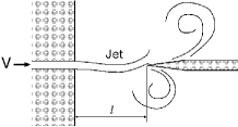
Figure 1: Edge tone

2.3 Phenomenological theory of air-reed instruments

The driving mechanism of air-reed instruments was first studied by Cremer & Ising, and Coltman as pioneer works[5, 6, 7, 8, 9], which have been followed by many authors[14, 15, 16]. Those studies have made differences in driving mechanism clear between the edge tone and the air-reed instrument with a resonator. It is turned out that there are two ways in which a pulsating jet drives a pipe, momentum drive and volume flow drive[1]. In the momentum drive, the jet is brought to rest by mixing and dissipation, and thereby generates an acoustic pressure which acts on an acoustic flow in the resonator. In the volume flow drive, the jet essentially contributes a volume flow which acts on the acoustic pressure at the open mouth, which is not zero because of the end correction. In the following, we mention the outline of driving mechanism and regenerative excitation mechanism of air-reed instruments according to the text book by Fletcher and Rossing[1].

2.3.1 Driving mechanism

The jet which emanates from a flue is disturbed by a uniform transverse acoustic-flow $v_{z}\exp(i\omega t)$ and forms an oscillating wave which propagates with a velocity $u$ and grows exponentially with a growth parameter $\mu$. The wave of jet propagating in $x$-direction is well approximated by the semi-empirical equation (also see Fig.2):

$$J(x)=-i\frac{v_{z}}{\omega}\bigl{\{}\exp(i\omega t)-\cosh(\mu x)\exp(i\omega(t-x/u))\bigr{\}}.$$

(5)

In the range $kd\gg 1$, where $d$ stands for the height of flue aperture, we can use approximations $u\sim V/2$ and $\mu\sim k$. Since they are available in a quite wide range, we always assume those approximations in the following. In this formula, the existence of edge, which plays the important role in formation of the jet oscillation, is ignored. Thus it should be considered that eq.(5) only gives the lowest order approximation of the jet motion.

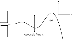
Figure 2: Jet oscillation

Taking into account the jet oscillation given by eq.(5), it is possible to make phenomenological formulation of that driving mechanism through which the jet acts on the pipe. As shown by Fig.3, after the jet of a steady velocity $V$ reaches the edge of the pipe, a fraction of its cross section $S_{j}$ enters the pipe. It is assumed that the fraction of jet blends with an acoustic flow in the volume between the cross sections M and P with a distance $\Delta x$ so that only acoustic motions survive in the other part of pipe beyond the cross section P. Under this assumption, the acoustic volume flow $U_{p}$ at the cross section P is expressed by

$$U_{p}=\frac{\rho V^{2}S_{j}}{S_{p}(Z_{p}+Z_{m})}+\frac{i\rho\omega\Delta LVS_{j}}{S_{p}(Z_{p}+Z_{m})},$$ (6)

where $Z_{m}=i\rho\omega\Delta L/S_{p}$ denotes the impedance at a frequency $\omega$ looking out from the plane M, $\Delta L$ the end correction at the open mouth, $Z_{p}$ the pipe impedance evaluated at the plane M and $S_{j}$ the area of the cross section of the pipe.

Two term in RHS of eq.(6) indicate two different drive mechanisms. The first constitutes the momentum drive and the second is the volume flow drive. In the situation $\omega\Delta L>V$, the second term is larger than the first so that the volume-flow mechanism dominates the momentum-drive mechanism. For our numerical calculations implemented in section4, substitution of representative values of the fundamental frequency of the pipe and the end correction of the open mouth, i.e., $\omega\sim 2\pi\times 913.1{\rm rad/s}$ and $\Delta L=0.005{\rm m}$, gives $\omega\Delta L=9.131\pi\sim 28.7{\rm m/s}$. Thus the volume-flow mechanism dominates if $V<28.7{\rm m/s}$. For the third harmonic at $2739.3{\rm Hz}$, the volume-flow mechanism governs the driving process in the range $V<86.1{\rm m/s}$. As shown later, the fundamental dominates for $V\leq 22{\rm m/s}$, while the third harmonic overcomes the fundamental for $V\geq 24{\rm m/s}$, then it is expected that the dominant mechanism exciting the sound wave in our numerical range ($2\leq V\leq 40{\rm m/s}$) is the volume flow drive.

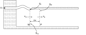
Figure 3: Pipe driven by jet

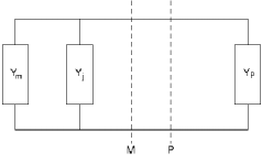
Figure 4: Equivalent circuit network

2.3.2 Regenerative excitation mechanism

Based on the analysis in the previous subsection, we can describe the sound excitation mechanism of air-reed instruments. To do this, we separate the system into a generator and a resonator by the plane, such as P or M. Make use of an equivalent circuit network (see Fig.4), we can determine the oscillating condition giving sound frequencies of the modes as functions of the jet velocity.

The stability condition of the network is given by

$$Y_{j}+Y_{m}+Y_{p}=0,$$ (7)

where $Y_{j}$ denotes the jet admittance obtained from the jet motion in eq.(5), which is given by

$$Y_{j}\sim\frac{VW}{\rho\omega^{2}\Delta L}\cosh{\mu l}\exp\Biggl{[}-i\Bigl{(}\frac{\omega l}{u}+\phi\Bigr{)}\Biggr{]}$$ (8)

with $\phi=\arctan\Bigl{(}\frac{V}{\omega\Delta L}\Bigr{)}$, the mouth admittance $Y_{m}$ is defined by $Y_{m}=1/Z_{m}=-i\frac{S_{p}}{\rho\omega\Delta L}$, and the pipe admittance $Y_{p}$ has the forms: $Y_{p}=-i\frac{S_{p}}{\rho c}\cot kL$ for an open end pipe with a length $L$ and $Y_{p}=i\frac{S_{p}}{\rho c}\tan kL$ for a closed end pipe.

It is convenient to separate the condition (7) into the real and imaginary parts

$${\rm Re}Y_{j}<0,$$ (9)

$${\rm Im}(Y_{j}+Y_{m}+Y_{p})=0.$$ (10)

Eq.(9) indicates that the jet must have a negative resistance as a power supplier that excites the system overcoming non-zero resistances of the mouth and pipe impedance, which are, however, ignored in this analysis. For the closed end pipe, the imaginary part (10) is rewritten as

$$-\frac{1}{\omega\Delta L}-\frac{V}{\omega^{2}\Delta Lh}\cosh{\mu l}~{}\sin\Biggl{[}\Bigl{(}\frac{\omega l}{u}+\arctan\Bigl{(}\frac{V}{\omega\Delta L}\Bigr{)}\Bigr{)}\Biggr{]}$$

$$~{}~{}~{}~{}~{}~{}~{}~{}~{}~{}~{}~{}~{}~{}~{}~{}~{}~{}~{}~{}~{}~{}~{}~{}~{}~{}~{}~{}~{}~{}~{}~{}~{}~{}~{}~{}+\frac{1}{c}\tan kL=0.$$ (11)

The ideal excitation is given by ${\rm Re}Y_{j}<0$ and ${\rm Im}Y_{j}=0$ so that the phase of $Y_{j}$ in eq.(8) takes $-\pi$, i.e., $\omega l/u=\pi-\phi$ and ${\rm Im}(Y_{m}+Y_{p})=0$. Since ${\rm Im}Y_{m}<0$, ${\rm Im}Y_{p}$ must takes a positive value. If the condition $\omega\Delta L/c\ll 1$ is satisfied, we obtain $kL\sim n\pi$ for the open end pipe and $kL\sim(n+1/2)\pi$ for the closed end pipe, which give the resonance conditions for the open and closed end pipes, respectively.

Fig.5 illustrates the frequency of excited sound wave as a function of the jet velocity $V$ given by eq.(2.3.2) for the closed end pipe together with the ideal condition $\omega l/u=\pi-\phi$ and the edge tone frequency in eq.(4) with $j=1$. The frequency of sound wave first increases in proportion to the jet velocity similar to the edge tone, but it is synchronized with the fundamental resonance, if the edge tone frequency comes near the fundamental frequency. Locking to the fundamental is continued until the edge tone frequency is close to the next resonance frequency. After that it jumps up to the next resonance and is synchronized with it, so the same process may be repeated every when the edge tone frequency reaches next one.

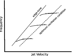
Figure 5: Oscillation frequency vs. jet velocity

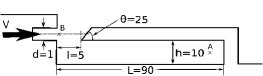
(a)     (b)

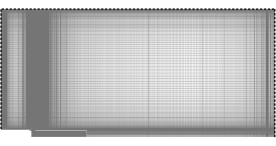
Figure 6: (color online) Model and mesh.  (a) Dimensions of 2D model (Unit of length :mm; Unit of angle:degree). (b) Numerical mesh. Dotted lines denote transparent walls.

3 Model and numerical scheme

3.1 Numerical model

For numerical analysis of air-reed instruments, we simultaneously calculate the dynamics of the jet flow and the sound field excited in a resonator. The sound speed $c$ of about $340{\rm m/s}$ is much higher than the jet velocity $V$, which is at most several tens in MKS units. For reproduction of sound, an extremely smaller time step is required compared with ordinary numerical calculations of fluid dynamics. On the other hand, spatial scales used for calculations of fluid dynamics with those vortices, some of which may be smaller than $1{\rm mm}$, are much less than wave lengths of sound, e.g., $34{\rm mm}$ even at $10{\rm kHz}$. Therefore, in the numerical calculation of air-reed instruments we must satisfy the both requirements, a sufficiently small time step to describe sound propagation and a spatial mesh finer enough to reproduce vortices in fluid. Further, particle velocities of sound (or energies of sound) are usually much less than those of the flow. It turns out that sound energies in living environment are $10^{-4}$ times as small as or smaller than those of fluid. It is not easy to numerically calculate with a high degree of accuracy sound propagation dissipating for a long distance.

To realize the calculation, we take a two dimensional (2D) model of a small air-reed instrument and concentrate our attention on dynamics in a near field of it. Taking a 2D model rather than a 3D model makes the number of grids necessary for the calculation reduce, which gives rise to diminishing elapse time, although some of important 3D effects might be lost.

Fig.6 (a) shows geometry of the 2D model we adopt, where $d$ denotes nozzle height, $l$ width of mouth aperture, $L$ pipe length, $h$ pipe height and $\theta$ edge angle, and those values are taken as shown in the figure. The model instrument is $9{\rm mm}$ in length thereby the fundamental frequency being estimated as $f_{0}\sim 913.1{\rm Hz}$ including the open end correction. The edge angle is fixed at $25^{\circ}$, at which we got the most stable oscillation in preliminary calculations. This angle value is in a suitable range for real instruments.

Table 1: Parameters of mesh

points	cells	faces
158,762	78,492	314,856

3.2 Numerical method

For numerical calculation, we use a compressible LES (Large eddy simulation), which is very popular in numerical simulations of aero-acoustics. Actually the scheme we adopt is the compressible LES solver, Coodles of OpenFOAM, provided as a free software by OpenCFD Ltd[35]. LES is very stable for a long time simulation, while it involves some ambiguities in boundary layers due to statistical assumption for dynamics of eddies smaller than a given grid size. It however makes sense in the statistical point of view.

As shown in Fig.6(b), the spatial area of the numerical mesh is taken large enough to include an acoustic field outside the instrument and parameters of the mesh are taken as shown in Table 1. The averages of pressure and temperature are taken as $p_{0}=100{\rm kPa}$ and $T_{0}=300{\rm K}$, respectively. The time step of numerical integration is $\Delta t=10^{-7}{\rm sec}$ and time evolution up to $0.1{\rm sec}$ is obtained. The velocity of the jet emanating from the flue $V$ is changed as a control parameter in the range $(2\leq V\leq 40{\rm m/s})$. Observations are done as follows. The acoustic pressure $p$ and air density $\rho$ are observed at the point A, distance of $10{\rm mm}$ from the right end of the pipe and on the center line of it. The vorticity $\omega$ in the jet flow is calculated at point B, distance of $1.6{\rm mm}$ right from the exit of the flue and on the center line of it.

4 Numerical results

4.1 Stable oscillation

In this subsection, we show numerical results of that oscillation at $V=12{\rm m/s}$ which is the most stable among oscillations observed in the whole range of $V$. Fig.7 (a) and (b) show the acoustic pressure oscillation observed at the point A and its power spectrum, respectively. For the calculation of the spectrum, initial transient oscillations ($0\leq t<0.01{\rm s}$) are omitted. The oscillation of the acoustic pressure in Fig.7 (a) is very stable with an almost constant pitch in the whole range of time ($0\leq t\leq 0.1{\rm s}$) except for a short initial transition. Its amplitude is gently undulated but reaches up several hundreds ${\rm Pa}$, which are much larger than normal acoustic pressures in the open air field. As shown in Fig.7(b), the main peak of the spectrum is very sharp and appears at $\nu=805.7{\rm Hz}$, which is less than the theoretical estimation of the fundamental resonance frequency $913.1{\rm Hz}$ by $107.4{\rm Hz}$. However, it rapidly approaches the resonance frequency with increase of $V$ as shown later. Thus it is considered that the oscillation at $V=12{\rm m/s}$ is almost locked on the fundamental resonance.

(a)

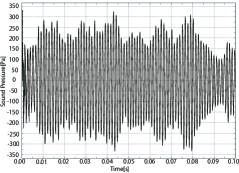
(b)

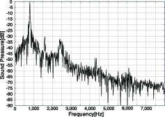
Figure 7: Acoustic pressure at point A. (a) Acoustic pressure oscillation. (b) Power spectrum.

(a)

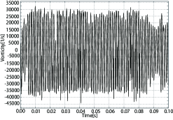
(b)

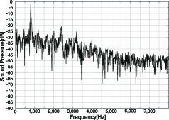
Figure 8: Vorticity at point B.  (a) Vorticity oscillation. (b) Power spectrum.

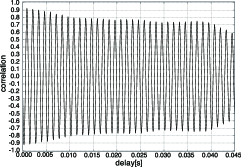
Figure 9: Correlation between sound pressure and jet vorticity.

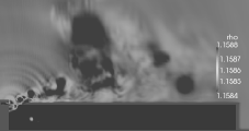
(a)      (b)

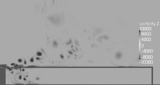
(c)      (d)

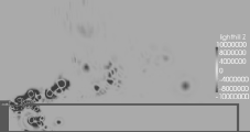
Figure 10: (color online) Spatial distributions of representative dynamical variables.  (a) Air density. (b) Flow velocity.  (c) Vorticity. (d) Lighthill’s sound source.

Fig.8 (a) and (b) show the vorticity fluctuation of jet observed at the point B and its power spectrum, respectively. The vorticity regularly oscillates like the acoustic pressure at the point A with the same fundamental frequency as shown in the power spectrum(see Fig.8 (b)). Fig.9 shows the mutual correlation function between the acoustic pressure ($0.01\leq t\leq 0.1{\rm s}$) and the vorticity ($0.01\leq t\leq 0.1{\rm s}$). The correlation changes periodically with the same fundamental frequency and does not decay for a long time. It means that there is a strong correlation between the jet motion and sound field in the resonator and so the jet motion is controlled rather by the pipe resonance than by its self-oscillation mechanism.

Fig.10 shows spacial distributions of characteristic dynamical variables at a certain time: air density, flow velocity, vorticity and Lighthill’s sound source. We used eq.(3) for the calculation of Lighthill’s sound source. Though it is not shown in a picture, the acoustic pressure distribution $p(x,t)$ is almost as same as the air density distribution $\rho(x,t)$. In the stationary oscillation regime, fluctuations of $\rho(x,t)$, more precisely $|\rho(x,t)-\rho_{0}|$, become much larger in the inside of pipe than in the outside as shown in Fig.10 (a).

In the velocity distribution in Fig.10(b), we see that eddies mainly arise from collision of the oscillating jet with the edge and are pouring into the inside or going to the outside of pipe. The eddies in the outside run along the wall of pipe being dissipated gradually. On the other hand, those in the inside roll up and make a large rotor or a few rotors near the mouth opening not spreading into more right hand side. No eddies apparently appear in the right 3/4 part of the pipe, in which the strong sound field dominates the flow. Such a rotor(s) always appears in stable oscillations and so the existence of the rotor(s) may affect the jet motion, though we do not touch details of the mechanism in this paper.

As shown in Fig.10(c), vorticity takes large (absolute) values along the upper and lower boundaries of jet and in areas of strong eddies rolled up. Lighthill’s sound source in Fig.10(d) almost overlaps with the vorticity distribution. This fact is supported by the main claim of the Powell-Howe vortex sound theory[4, 18, 19] that the major part of Lighthill’s sound sources is of contribution of vortices. The sound sources along the jet periodically oscillate reflecting the motion of jet. On the other hand, the other sound sources mainly located on large eddies behave rather irregularly in time evolution due to irregular motions of the eddies. This fact combined with the fact that the vorticity of jet is strongly correlated with the sound field excited in the pipe suggests that the main mechanism driving the sound field in the pipe at $V=12{\rm m/s}$ is ’volume flow drive’ rather than ’momentum drive’. This suggestion is also supported by the theoretical prediction discussed in subsection 2.3.1.

4.2 Frequency change with jet velocity

In this subsection, we discuss change of characteristic frequencies of sound waves excited in the pipe, i.e., spectrum peaks of fundamental and first overtone, with increase of the jet velocity $V$. In Fig.11, we show characteristic frequencies of the acoustic pressure at the point A as functions of V in the range ($2\leq V\leq 40{\rm m/s}$). For comparison, resonance frequencies of the pipe estimated theoretically and the edge tone frequency given by eq.(4) with $j=1$ are also depicted in Fig.11. The fundamental frequency of the acoustic pressure is observed in the whole range of $V$, but the first overtone is identified only at high velocities, $V\geq 18{\rm m/s}$.

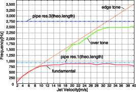
Figure 11: (color online) Changes of oscillation frequencies with jet velocity. The lines labeled ’pipe res.1’ and ’pipe res.3’ respectively indicate the frequencies of fundamental and 3rd harmonics resonances estimated theoretically.

In the low velocity regime, ($V\leq 8{\rm m/s}$), the fundamental frequency of acoustic pressure increases as that of the edge tone, namely it is proportional to $V$. Hence the jet motion is little affected by the pipe resonance and almost keeps its natural oscillation. For example, the acoustic pressure and its power spectrum at $V=4{\rm m/s}$ are shown in Fig.12 (a) and (b), respectively. The acoustic pressure oscillates somewhat regularly at $\nu_{0}=341.8{\rm Hz}$ with very small amplitudes compared with those at $V=12{\rm m/s}$. However, the power spectrum shown in Fig.12(b) is something interesting: the first overtone peak at $\nu_{1}=659.2{\rm Hz}$ accompanied by smaller side peaks in a upper range is observed. This broad band of peaks seems to be affected by the pipe resonance. Indeed, the fundamental frequency $\nu_{0}$ is slightly less than half of fundamental resonance frequency, so a broad band of peaks accompanying the overtone can appear near the fundamental resonance frequency. As shown in Fig.12 (c), the correlation between the acoustic pressure and vorticity oscillates in a regular manner but gradually decays to an oscillation much smaller than that at $V=12{\rm m/s}$. Then it is considered that the interaction between the generator and resonator is small in this regime. Namely an unidirectional interaction from the generator to the resonator dominates the operation with less feedback from the resonator, thereby being out of resonance.

(a)

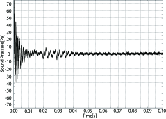
(b)

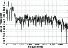
(c)

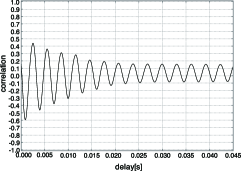
Figure 12: Oscillation at $V=4{\rm m/s}$.  (a) Acoustic pressure. (b) Power spectrum. (c) Correlation with vorticity at point B.

In the middle range, ($10\leq V\leq 22{\rm m/s}$), oscillations of sound wave locking on the fundamental pipe resonance are observed. The frequency of oscillation is fairly lower than that of fundamental resonance at $V=10{\rm m/s}$, but it quickly approaches the frequency of the resonance with increase of $V$. The oscillations are very stable in the range ($10\leq V\leq 16{\rm m/s}$) and the most stable one is observed at $V=12{\rm m/s}$ as shown in the previous subsection. So the oscillation is most stabilized just above the value of $V$ at which the jet motion starts synchronizing with the pipe resonance. In the range ($18\leq V\leq 22{\rm m/s}$), oscillations, however, become slightly unstable. Namely some amplitude modulations occur in long term evolutions, though we do not show results. In the spectra of those oscillations, there observes a peak corresponding to the edge tone frequency at the present velocity $V$. Further smaller peaks whose frequencies are nearly equal to the third harmonic of the pipe are often observed. It is considered that competition among the resonances and edge tone, i.e., inherent oscillation of the jet, occurs, but the fundamental still dominates the others, though its oscillation is somewhat disturbed.

In the high velocity range, ($V\geq 24{\rm m/s}$), first overtone peaks likely to be the third harmonic are clearly observed in the spectra of acoustic pressure. The frequency of the first overtone peak increases mostly proportional to the jet velocity like the edge tone in the range $18\leq V\leq 24{\rm m/s}$ but almost converges to a constant value in the range $V\geq 32{\rm m/s}$, e.g., $\nu_{1}=2490.2{\rm Hz}$ at $V=36{\rm m/s}$, although it is considerably lower than the theoretical estimation of the third harmonic, $2739.3{\rm Hz}$. Then the oscillation would start to be synchronized with the third harmonic around $V=24\sim 26{\rm m/s}$. Indeed, the peak height of the first overtone is increasing with increase of $V$ and becomes larger than that of the fundamental for $V\geq 24{\rm m/s}$ (for example see Fig.13(b) at $V=36{\rm m/s}$). Further the wave form of acoustic pressure changes to that of the third harmonic for $V\geq 24{\rm m/s}$. Fig.13(a) shows the time evolution of the acoustic pressure at $V=36.0{\rm m/s}$. It oscillates almost periodically with very strong amplitudes, sometimes exceeding $1{\rm kPa}$. As shown in Fig.13(c), the correlation between the sound pressure at the point A and the vorticity at the point B behaves in a regular manner and does not decay in a long term. In conclusion, it can be said that the transition from the fundamental to the third harmonic occurs around $V=24{\rm m/s}$.

(a)

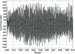
(b)

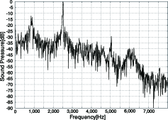
(c)

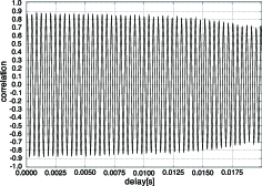
Figure 13: Oscillation at $V=36{\rm m/s}$. (a) Acoustic pressure. (b) Power spectrum. (c) Correlation with vorticity at point B.

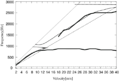
Figure 14: Comparison of the numerical result with the theoretical prediction in change of frequencies with the jet velocity.

We compare our numerical result with the theoretical prediction introduced in section 2.3.2. Fig.14 shows the velocity-frequency curves (broken lines) given by eq.(2.3.2) at parameter values adjusted to our numerical calculation: $l=5{\rm mm}$, $\Delta L=9{\rm mm}$, $h=10{\rm mm}$, $L=90{\rm mm}$, $c=340{\rm m/s}$, $\mu l=\pi$. However, we need to rescale the argument of sinusoidal function in eq.(2.3.2) as $u/l=0.8V/l$ to make it be adjusted to the edge tone equation (4) and also to our numerical result, while it is usually taken as $u/l\leq 0.5V/l$. The curves of eq.(2.3.2) are drawn only in the area limited by the two dotted lines given by ${\rm Re}Y_{j}=0$, in which the jet has a negative value in resistance, the necessary condition to excite the instrument. The chain line stands for the optimum oscillation condition ${\rm Im}Y_{j}=0$. For comparison, the velocity-frequency curves obtained numerically, which are the sames as those in Fig.11, are also drawn by solid lines.

Our numerical result shows good agreement with the theoretical prediction in three characteristic ranges: oscillations of the edge tone in the low velocity range, locking to the fundamental resonance in the middle range, and transition and locking to the third harmonic in the high range. It is expected that the optimum oscillations of the first and third harmonics occur at intersections of the corresponding branches of eq.(2.3.2) with the line ${\rm Im}Y_{j}=0$, respectively. The intersection appears just after locking to the first or third harmonics starts. The fact that the optimum oscillation of the fundamental is observed numerically at $V=12{\rm m/s}$ well supports the validity of theoretical prediction. A well sustained third harmonic, e.g., at $V=36{\rm m/s}$, is also observed near the intersection of the third harmonic.

Here, we explain why we take the parameter $u/l$ as $u/l=0.8V/l$ instead of $u/l=0.5V/l$ in order to calculate the velocity-frequency curves and optimum line. According to experiments and the semi-empirical theory, the velocity of jet wave $u$ should take a value in the range $u\leq 0.5V$. However, even at $u=0.5V$, the velocity-frequency curves given by eq.(2.3.2) lean to the right more. As a result, the curves are markedly shifted from the edge tone line in a low velocity range and the onset point of locking to the fundamental is estimated as $V\sim 20{\rm m/s}$. Then those curves apparently go out of our numerical results and also out of Brown’s edge tone equation. Taking into account the fact that the existence of the edge is ignored in framing the jet model in that theory (see 2.3.1), it is considered that such extent of modification is still within an acceptable limit. It is rather surprised that the semi-empirical theory shows quantitatively good agreement with full numerical calculations with such a slight modification.

Finally note that as discussed in subsection 2.3.1, it is predicted that the volume-flow mechanics dominates in excitation of sound waves not only in the range of the fundamental but also in the range of the third harmonic. We think that this prediction is probably true and is partially supported by the observation that the correlation between the acoustic pressure and the vorticity of the jet behaves regularly without remarkable decays in the ranges of $V$, in which the fundamental and the third harmonic are well sustained. Further it is also confirmed in preliminary calculations that the correlation becomes more unstable, if the vorticity is observed at a point in the relaxation area between the planes M and P in Fig.3, i.e., momentum driving area, because motions of eddies in this region are more irregular than the jet oscillation.

5 Summary and discussion

In this paper, we have reported on the numerical analysis of a 2D air-reed instrument with the compressible LES. As a result, vibrations of the air-reed instrument are well reproduced by using the compressible LES. Especially, some characteristic features of the air reed instrument obtained numerically show good agreement with those given by the theoretical prediction as well as experimental results[1, 8, 9, 14, 15, 22]. The characteristic features reproduced are as follows.

When the velocity is small enough, the inherent jet oscillation radiating the edge tone is predominant so that the oscillation frequency of sound excited in the pipe is almost proportional to the jet velocity. However, the jet oscillation is synchronized with the fundamental resonance of the pipe when the frequency of edge tone approaches that of the fundamental resonance with increase of the jet velocity. The synchronization with the fundamental resonance continues until the frequency of edge tone reaches that of the first overtone, i.e., 3rd harmonic in our case. Then the synchronization is turned off and the transition to the 3rd harmonic arises, namely the frequency locking to the 3rd harmonic takes place.

Based on the results of this paper, we are able to proceed to study the acoustic mechanism of the air-reed instrument comprehensively. With help of the Lighthill theory[17] and/or Powell-Howe vortex sound theory[19, 18, 4], the place of sound sources in turbulence will be detected clearly and their behavior will be characterised in terms of aero-dynamics and nonlinear dynamics. The following problems and questions should be investigated. The questions which mechanism, volume-flow mechanism or momentum drive mechanism[5, 6, 7, 8, 9, 14, 15, 16], dominates at a given playing condition and what change occurs with change of the playing condition, e.g., with the jet velocity, should be answered clearly. It should be also clarified what kind of influence the resonance of the pipe exerts on the motion of the jet, because it must be the key to understand the synchronization mechanism between the jet flow and pipe resonance, the key mechanism of wind instruments different from the edge tone.

To analyze more realistic behavior of instruments, the numerical analysis of 3D models is needed. In a preliminary calculation, we have succeeded to numerically reproduce acoustic oscillations of the ocarina with a 3D model[36]. It is considered that the ocarina uses the Helmholtz resonance caused by an elastic property of air instead of the pipe resonance. Then, it is quite interesting to consider the problem how different acoustic mechanisms work for different types of resonator with comparing numerical data of the ocarina with that of a 3D model of the instrument with a resonance pipe. Before that it is of course necessary to clarify differences between the 2D and 3D models.

- [1] N. H. Fletcher and T. D. Rossing, The Physics of Musical Instruments, 2nd Edition (Springer-Verlag, New York 1998).
- [2] A. Hirschberg, “Aero-acoustics of Wind instruments.” in Mechanics of Musical Instruments, Eds. A.Hirschberg, J.Kergomard and G.Weinreich. (Springer-Verlag, Vienna and New York 1995), pp.291-369.
- [3] G. B. Brown, “The vortex motion causing edge tones,” Proc. Phys. Soc., London XLIX 493-507 (1937).
- [4] M. S. Howe, Acoustics of Fluid-Structure Interactions, (Cambridge Univ. Press, 1998).
- [5] L. Cremer and H. Ising, “Die selbsterregten Schwingungen von Orgelpfeifen,” Acustica 19 143-153 (1967).
- [6] J. W. Coltman, “Sounding mechanism of the flute and organ pipe,” J. Acoust. Soc. Am. 44 983-992 (1968).
- [7] J. W. Coltman, “Acoustics of the flute,” Physics Today 21 25-32 (1968).
- [8] J. W. Coltman, “Jet driven mechanisms in edge tones and organ pipes,” J. Acoust. Soc. Am. 60 725-733 (1976).
- [9] J. W. Coltman, “Momentum transfer in jet excitation of flute-like instruments,” J.Acoust. Soc. Am. 69 1164-1168 (1981).
- [10] N. H. Fletcher and S. Thwaites, “Wave propagation on an acoustically perturbed jet,” Acustica 42 323-334 (1979).
- [11] S. Thwaites and N. H. Fletcher, “Wave propagation on turbulent jets,” Acustica 45 175-179 (1980).
- [12] S. Thwaites and N. H. Fletcher, “Wave propagation on turbulent jets. II. Growth,” Acustica 51 44-49 (1982).
- [13] N. H. Fletcher and S. Thwaites, “The physics of organ pipes,” Scientific American 248 84-93 (1983).
- [14] N. H. Fletcher, “Jet-drive mechanism in organ pipes,” J. Acoust. Soc. Am. 60 481-483 (1976).
- [15] S. A. Elder, “On the mechanism of sound production on organ pipes,” J. Acoust. Soc. Am. 54 1554-1564 (1973).
- [16] S. Yoshikawa and J. Saneyoshi, “Feedback excitation mechanism in organ pipes,” J. Acoust. Soc. Jpn. (E) 1 175-191 (1980).
- [17] M. J. Lighthill, “On sound generated aerodynamically. Part I: General theory,” Proc. Roy. Soc. London A211 564-587 (1952).
- [18] A. Powell, “Theory of vortex sound,” J.Acoust. Soc. Am. 36 177-195 (1964).
- [19] M. S. Howe, “Contributions to the theory of aerodynamic sound with appliction to excess jet noise an the theory of the flute,” J. Fluid Mech. 71 625-673 (1975).
- [20] M. P. Verge, R. Caussë, B. Fabre, A. Hirschberg, A. P. J. Wijnands, and A. van Steenbergen, “Jet oscillations and jed drive in recorder-like instruments,” Acta acoustica 2 403-419 (1994).
- [21] M. P. Verge, B. Fabre, W. E. A. Mahu, A. Hirschberg, R. R. van Hassel, A. P. J. Wijnands, J. J. de Vries, and C. J. Hogendoorn “Jet formation and jet velocity fluctuations in a flue organ pipe,” J. Acoust. Soc. Am. 95 1119-1132 (1994).
- [22] B. Fabre, A. Hirschberg, A. P. J. Wijnands, “Vortex shedding in steady oscillation of a flue organ pipe,” Acta acustica, Acoustica 82 863-877 (1996).
- [23] M. P. Verge, B. Fabre, and A. Hirschberg, “Sound production in recorderlike instruments. I. Dimensionless amplitude of the internal acoustic field,” J. Acoust. Soc. Am. 101 pp. 2914-2924 (1997).
- [24] M. P. Verge, A. Hirschberg, and R. Caussë, “Sound production in recorderlike instruments. II. A simulation model,” J. Acoust. Soc. Am. 101 2925-2939 (1997).
- [25] S. Dequand, J. F. H. Willems, M. Leroux, R. Vullings, M. van Weert, C. Thieulot, and A. Hirschberg, “Simplified models of flue instruments: Influence of mouth geometry on the sound source,” J. Acoust. Soc. Am. 113 1724-1735 (2003).
- [26] S. Yoshikawa, “A pictorial analysis of jet and vortex behaviours during attack transients in organ pipe models,” Acta acustica, Acustica 86 623-633 (2000).
- [27] H. Kühnelt, “Simulating and sound generation in flutes and flue pipes with the Lattice-Boltzmann-Method,” Proc. of ISMA 2004, Nara Japan, pp.251-254.
- [28] J. Tsuchida, T. Fujisawa, and G. Yagawa, “Direct numerical simulation of aerodynamic sounds by a compressible CFD scheme with node-by-node finite elements,” Computer Methods in Applied Mechanics and Engineering 195 1896-1910 (2006).
- [29] A. Bamberger, “Vortex sound of the flue,” Proceedings of ISMA2007, Barcelona Spain, (CD-ROM ISBN:978-84-934142-1-4), 1-S1-5.
- [30] E. D. Lauroa, S. D. Martinob, E. Espositoc, M. Falangad, and E. P. Tomasinie “Analogical model for mechanical vibrations in flue organ pipes inferred by independent component analysis,” J. Acoust. Soc. Am. 122 2413-2424 (2007).
- [31] O. Coutier-Delgosha, J. F. Devillers, and A. Chaigne, “Edge-tone instability: Effect of the gas nature and investigation of the feedback mechanism,” Acta. Acust. Acust. 92 236–246 (2006).
- [32] J. Braasch, “Acoustical measurements of expression devices in pipe organsa,” J. Acoust. Soc. Am. 123 1683-1693 (2008).
- [33] H. J. Auerlechner, T. Trommer, J. Angster, and A. Miklós “Experimental jet velocity and edge tone investigations on a foot model of an organ pipe,” J. Acoust. Soc. Am. 126 878-886 (2009).
- [34] C. Wagner, T. Hüttl, and P. Sagaut, eds. Large-Eddy Simulation for Acoustics, (Cambridge Univ. Press, New York, 2007).
- [35] http://www.openfoam.com/
- [36] T. Kobayashi, T. Takami, M. Miyamoto, K. Takahashi, A. Nishida, and M.Aoyagi, “3D Calculation with Compressible LES for Sound Vibration of Ocarina,” Open Source CFD International Conference 2009, November 12-13th, Barcelona, Spain (CD-ROM).