Counting Statistics in Nanoscale Junctions.

Abstract

We present first-principles calculations for the third moment of the current in atomic-scale junctions. We calculate this quantity in terms of the effective single-particle wave-functions obtained self-consistently within the static density-functional theory. As an example, we investigate the relations among the conductance, the second and third moments of the current for carbon-atom chains of various lengths bridging two metal electrodes. We find that the conductance, the second-order and the third-order Fano factors show odd-even oscillation with the number of carbon atoms with the third-order Fano factor positively correlated to the conductance.

Nanoscale electronics has generated a tremendous wave of scientific interest in the past decade due to prospects of device-size reduction offered by atomic-level control of certain physical properties Aviram . In addition, it has spurred great interest in the fundamental understanding of quantum transport book . One of these fundamental questions relates to the moments of the current. For instance, the second moment - shot noise - defines the quantum fluctuations of the current at zero temperature due to the quantization of charge. Shot noise reaches the classical limit $2eI$, where $e$ is the electron charge and $I$ is the average current Schottky , when electrons in a conductor drift in a completely uncorrelated way as described by a Poissonian distribution of current events. On the other hand, in the presence of a junction with a narrow constriction, electrons, shot noise can be expressed as $S_{2}\propto\sum_{n}T_{n}\left(1-T_{n}\right)$ in terms of the transmission probabilities of each eigen-channel $T_{n}$ Blanter . It is a powerful tool for the exploration of quantum statistics of non-equilibrium electrons Ruitenbeek1 ; Natelson ; MRE ; Agra ; chen ; Lagerqvist ; chen1 ; Yao and may provide a means to explore also local temperature effects in nano-structures chen1 . In fact, it has been recently employed to characterize the signature of molecules/atomic wires in junctions Ruitenbeek1 ; Kiguchi ; Natelson .

The higher moments of the current (although more difficult to measure and calculate) provide deeper insight into the statistics of charge dynamics, and are therefore more refined tools to characterize the signature of molecules in junctions. However, no studies have considered higher moments of the current in truly atomic-scale systems. To address this issue, we have developed a theoretical approach that combined with static density functional theory (DFT), which allows us to compute correlations up to the third moment of the current in atomic junctions.

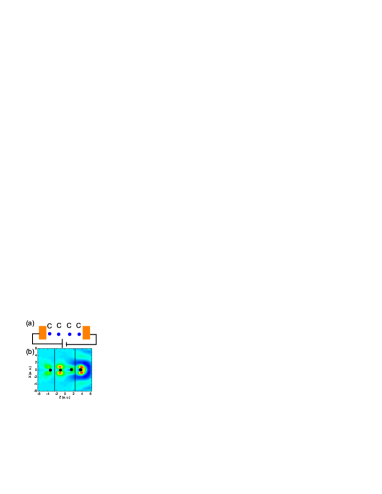
Figure 1: (color online) (a) Schematic of the four-carbon atomic junction. (b) The spacial distribution of partial charge density for electrons with energies near the Fermi levels shows $\pi$-orbital characters at $V_{B}=0.01$ V. Vertical black lines correspond to the edges of the jellium model and circles correspond to atomic position.

We have then investigated the relation between the conductance, the second moment (or shot noise, $S_{2}$), and the third moment of the current (we denote it with $S_{3}$) for a prototypical nanojunction consisting of an atomic chain with different number of carbon atoms connecting two metal electrodes as shown in Fig. 1(a). This is not just an academic example since carbon is a versatile element capable of forming diverse structures including diamond, graphite, fullerenes, nanotubes and graphene. Recently, experimentalists have shown the possibility to form carbon atomic chains from graphite using a transmission electron microscope Jin . The carbon atom chains have regularly patterned electronic structures as a function of the number of carbon atoms Avouris . In this regard, they are among the few model systems in which theory and experiments can be reasonably compared.

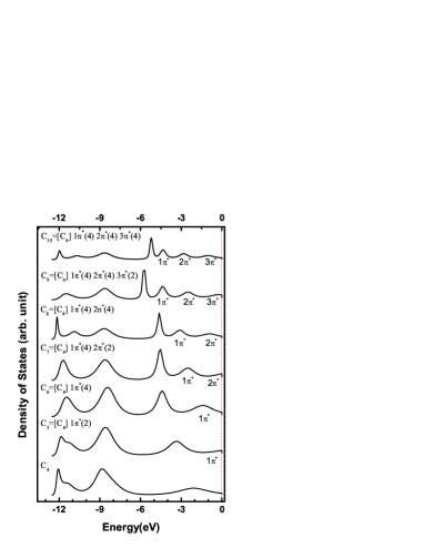
Figure 2: (color online) The density of states in the continuum region for N-atom carbon chains sandwiched between two metal electrodes at $V_{B}=0.01$ V. Zero of energy corresponds to the left Fermi level.

Let us then consider a system at steady state subject to a bias $V_{B}=(E_{FR}-E_{FL})/e$, where $E_{FR}$ and $E_{FL}$ are the right and left electrochemical potential, respectively. The system is described by the field operator

$$\hat{\Psi}=\sum_{\alpha,E,\mathbf{K}}a_{E\mathbf{K}}^{\alpha}\left(t\right)\Psi_{E\mathbf{K}}^{\alpha}\left(\mathbf{r}\right),$$ (1)

where $\alpha=L$ or $R$; $a_{E\mathbf{K}}^{L(R)}\left(t\right)=\exp(-i\omega t)a_{E\mathbf{K}}^{L(R)}$; and $a_{E\mathbf{K}}^{L(R)}$ is the annihilation operators of electrons incident from the left (right) reservoir, satisfying the anti-commutation relations

$$\{a_{E_{1}\mathbf{K}_{1}}^{\alpha},a_{E_{2}\mathbf{K}_{2}}^{\beta{\dagger}}\}=\delta_{\alpha\beta}\delta\left(E_{1}-E_{2}\right)\delta(\mathbf{K}_{1}-\mathbf{K}_{2}),$$ (2)

where $\beta=L$ or $R$. The single-particle wave functions $\Psi_{E\textbf{K}}^{L(R)}$, describe electrons with energy E and momentum K incident from the left (L) and right (R) electrodes are later computed self-consistently in the framework of DFT chen ; DiVentra2 ; Lang .

The current operator is defined as

$$\hat{I}(z,t) = \frac{e\hbar}{mi}\sum_{E_{1}E_{2}}\sum_{\alpha\beta}\int d\mathbf{r\bot}\int d\mathbf{K}_{1}\int d\mathbf{K}_{2}$$ (3)

$$\cdot e^{i(E_{1}-E_{2})t/\hbar}a_{E_{1}\mathbf{K}_{1}}^{\alpha{\dagger}}a_{E_{2}\mathbf{K}_{2}}^{\beta}\tilde{I}_{E_{1}\mathbf{K}_{1},E_{2}\mathbf{K}_{2}}^{\alpha\beta}(\mathbf{r}),$$

where

$$\tilde{I}_{E_{1}\mathbf{K}_{1},E_{2}\mathbf{K}_{2}}^{\alpha\beta}\left(\mathbf{r}\right)=\left(\Psi_{E_{1}\mathbf{K}_{1}}^{\alpha}\right)^{\ast}\nabla\Psi_{E_{2}\mathbf{K}_{2}}^{\beta}-\nabla\left(\Psi_{E_{1}\mathbf{K}_{1}}^{\alpha}\right)^{\ast}\Psi_{E_{2}\mathbf{K}_{2}}^{\beta}.$$

At zero temperature, the average of current operator gives the first moment,

$$<\hat{I}>=\frac{e\hbar}{mi}\int_{E_{FL}}^{E_{FR}}dE\int d\mathbf{r_{\bot}}\int d\mathbf{K}\tilde{I}_{E\mathbf{K},E\mathbf{K}}^{R,R}\left(\mathbf{r}\right),$$ (4)

where the following expectation values have been used:

$$<a_{E_{1}\mathbf{K}_{1}}^{\alpha{\dagger}}a_{E_{2}\mathbf{K}_{2}}^{\beta}>=\delta_{\alpha\beta}\delta\left(E_{1}-E_{2}\right)\delta(\mathbf{K}_{1}-\mathbf{K}_{2})f_{E}^{\alpha},$$ (5)

with $f_{E}^{L\left(R\right)}$ the Fermi-Dirac distribution function in the left (right) electrode.

We note that our wave-functions as obtained in the framework of DFT calculations describe noninteracting electrons, where the effective single-particle wavefunctions have boundary conditions describing electrons that are partially transmitted and partially reflected. Unlike the formalism developed in, e.g., Ref. Blanter , which has in-out ordering, the current operator defined in Eq. (4) describes steady-states current where the time ordering is not involved. Therefore, the current correlation functions are defined in the time-unordered way ,

$$S_{2}(\omega)=2\pi\hbar\int d(t_{1}-t_{2})e^{i\omega(t_{1}-t_{2})}<\Delta\hat{I}(t_{1})\Delta\hat{I}(t_{2})>,$$ (6)

and

$$S_{3}(\omega,\omega^{\prime})=(2\pi\hbar)^{2}\int d(t_{1}-t_{3})\int d(t_{2}-t_{3})e^{i\omega(t_{1}-t_{3})}e^{i\omega^{\prime}(t_{2}-t_{3})}<\Delta\hat{I}(t_{1})\Delta\hat{I}(t_{2})\Delta\hat{I}(t_{3})>,$$ (7)

where $\triangle\hat{I}(t)=\hat{I}(t)-\left\langle\hat{I}\right\rangle$; $S_{2}(\omega)$ and $S_{3}(\omega,\omega^{\prime})$ are the two- and three-current spectral functions, respectively.

The zero-frequency 2nd and 3rd moment of the steady-state current can be defined as $S_{2}=S_{2}(\omega=0)$ and $S_{3}=S_{3}(\omega=0,\omega^{\prime}=0)$,

$$S_{2}(z_{1},z_{2})=2\pi\hbar(\frac{e\hbar}{mi})^{2}\int_{E_{FL}}^{E_{FR}}dE\int d\textbf{r}_{1\bot}\int d\textbf{r}_{2\bot}\int d\textbf{K}_{1}\int d\textbf{K}_{2}\tilde{I}_{E\textbf{K}_{1},E\textbf{K}_{2}}^{RL}(\textbf{r}_{1})\tilde{I}_{E\textbf{K}_{2},E\textbf{K}_{1}}^{LR}(\textbf{r}_{2}),$$ (8)

and

$$\begin{split}S_{3}(z_{1},z_{2},z_{2})=&(2\pi\hbar)^{2}(\frac{e\hbar}{mi})^{3}\int_{E_{FL}}^{E_{FR}}dE\int d\textbf{r}_{1\bot}\int d\textbf{r}_{2\bot}\int d\textbf{r}_{3\bot}\int d\textbf{K}_{1}\int d\textbf{K}_{2}\int d\textbf{K}_{3}\\ &[\tilde{I}_{E\textbf{K}_{1}E\textbf{K}_{2}}^{RL}(\textbf{r}_{1})\tilde{I}_{E\textbf{K}_{2}E\textbf{K}_{3}}^{LL}(\textbf{r}_{2})\tilde{I}_{E\textbf{K}_{3}E\textbf{K}_{1}}^{LR}(\textbf{r}_{3})-\tilde{I}_{E\textbf{K}_{1}E\textbf{K}_{3}}^{RL}(\textbf{r}_{1})\tilde{I}_{E\textbf{K}_{2}E\textbf{K}_{1}}^{RR}(\textbf{r}_{2})\tilde{I}_{E\textbf{K}_{3}E\textbf{K}_{2}}^{LR}(\textbf{r}_{3})].\end{split}$$ (9)

where the expectation values in Eqs. (6) and (7) have been calculated using the Wick-Bloch-De Dominicis theorem Kubo ,

$$<\hat{A}_{n}\hat{A}_{n-1}\cdots\hat{A}_{1}>=\left\{\begin{array}[]{c}0\text{, for }n=odd\text{,}\\ \sum_{m=1}^{n-1}\eta^{n-m-1}<\hat{A}_{n}\hat{A}_{m}><\hat{A}_{n-1}\cdots\hat{A}_{m+1}\hat{A}_{m-1}\cdots\hat{A}_{1}>\text{, \ for }n=even\text{,}\end{array}\right.$$ (10)

where $\hat{A}_{i}$ denotes either creation or annihilation operators and $\eta=-1(1)$ for Fermions (Bosons). We note that alternative definitions of Fourier transform, e.g., the integrals with respect to $(t_{1}-t_{2})$ and $(t_{2}-t_{3})$ in Eq. (6) and (7) may lead to different parametrization of frequencies $\omega$ and $\omega^{\prime}$ in the spectral functions. However, in the case of the steady-state current where $\omega=\omega^{\prime}=0$, the zero-frequency current correlations are independent of the choices of Fourier transform. We also note that Eq. (8) leads to the relations $S_{2}^{RR}=S_{2}^{LL}=-S_{2}^{LR}=-S_{2}^{RL}$, where $S_{2}^{RR}=S_{2}(z\rightarrow\infty,z\rightarrow\infty)$, $S_{2}^{LL}=S_{2}(z\rightarrow-\infty,z\rightarrow-\infty)$, $S_{2}^{LR}=S_{2}(z\rightarrow-\infty,z\rightarrow\infty)$, and $S_{2}^{RL}=S_{2}(z\rightarrow\infty,z\rightarrow-\infty)$, which are a consequence of current conservation. Similarly, Eq. (9) leads to

$$S_{3}^{R(R,L)R}=S_{3}^{L(R,L)L}=-S_{3}^{L(R,L)R}=-S_{3}^{R(R,L)L},$$ (11)

For a single-channel tunnel junction with transmission probability $T$, the first, second, and third moment of current are given by $I\propto T$, $S_{2}\propto T(1-T)$, and $S_{3}\propto-2T^{2}(1-T)$, respectively. The result of the unordered third moment is consistent with the results of time-unordered three-current correlations derived by other groups Salo ; Bachmann . Finally, we define the second- and third-order Fano factors (which is dimensionless) in the small bias regime for steady-state currents as $F_{2}=S_{2}/(2eI)$ and $F_{3}=S_{3}/[(2e)^{2}I]$, respectively. As a direct result, for the single-channel junction $G\propto T$, $F_{2}\propto(1-T)$, and $F_{3}\propto-2T(1-T)$, respectively.

As an example, we have investigated the counting statistics in linear atomic chains formed by four to ten carbon atoms (denoted as C4 to C10) bridging between two metal electrodes modeled as electron jellium ($r_{s}=2$). The distances between two neighboring carbon atoms are $2.5$ a. u., and the end atoms of the chain are fixed at $1.4$ a. u. inside the positive background edge of the electron jellium as shown in Fig. 1(b) Avouris . As it was found in Ref. Avouris when the length of the wire is increased by one carbon atom, two electrons are added to the $\pi^{*}$-orbital as shown in Fig. 2. The odd-numbered chains have a higher conductance due to half-filled $\pi^{*}$-orbital while the even-numbered chains have a lower conductance due to a full-filled $\pi^{*}$-orbital at the Fermi levels, as shown in the upper panel of Fig. 3. In the middle and lower panels of Fig. 3 we show the influence of the number of carbon atoms on the second-order $F_{2}$ and the third-order Fano factor $F_{3}$, respectively, in the linear response regime ($V_{B}=0.01$ V). We observe that $F_{2}$ and $F_{3}$ both display odd-even oscillation with the number of carbon atoms.

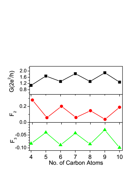
Figure 3: (color online) Conductance [(black) square; top panel], the second-order Fano factor [(red) circle; middle panel], and the third-order Fano factor [(green) triangle; bottom panel] of the atomic wires as a function of the number of carbon atoms in the wire at $V_{B}=0.01$ V.

In order to better understand the relation among the moments of counting statistics in the carbon atom chains, we have investigated the differential conductance (defined as $G=\partial I/\partial V$), the differential second-order Fano factor [defined as $F_{2}=(1/2e)\partial S_{2}/\partial I$], and the differential third-order Fano factor [defined as $F_{3}=(1/2e)^{2}\partial S_{3}/\partial I$] for the C4 and C5 wires in the non-linear response regime. We observe that the differential conductance of C4 chain increases as the applied bias increases, while the differential conductance of C5 chain decreases as the applied bias increases, as shown in the top panels of Figure 4(a) and (b), respectively. The increase (decrease) of differential conductance with the biases for the C4 (C5) chain is due to the half-filled (full-filled) $\pi^{*}$ orbital at the Fermi level, where more (less) states are included in the current-carrying energy window created by increasing biases. The bottom panels of Fig. 4(a) and (b) show that conductance and $F_{3}$ are strongly positively correlated indicating that the dominant eigen-channels for counting statistics have transmission probabilities $T>0.5$.

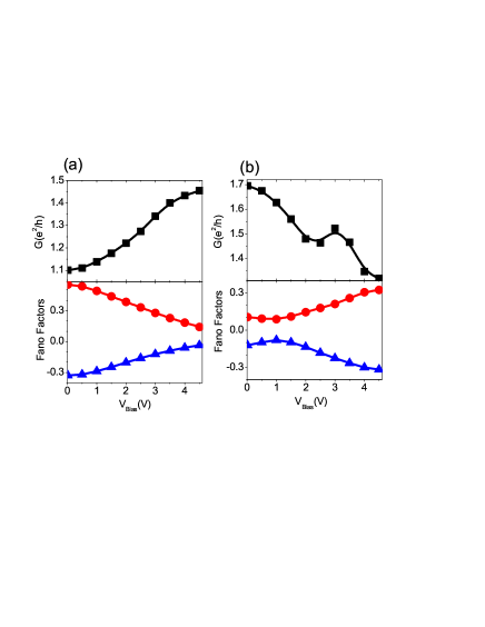
Figure 4: (color online) (a) For four-carbon atom wire and (b) for five-carbon atom wire: the differential conductance [(black) square; top panel], the second-order differential Fano factor [(red) circle; bottom panel], and the three-order differential Fano factor [(blue) triangle; bottom panel] vs. bias.

In conclusion, we have calculated the third moment of the current within DFT that allows the study of counting statistics at the atomic level. As an example, we have investigated the relation among conductance, second and third moments of the current for carbon chains of different length. In the linear response regime, conductance, second and third moments show odd-even oscillations with the number of carbon atoms, which is mainly due to the orderly patterned electronic structure of carbon-atom chains. In the nonlinear regime, the conductance increases (decreases) as bias increases in even- (odd-) numbered carbon atom chains. We observe that $F_{3}$ and differential conductance are significantly positively correlated, thus showing that third-order Fano factor provides more information than the second-order Fano factor regarding the transmission probabilities of eigen-channels.

The authors thank MOE ATU, NCHC, National Center for Theoretical Sciences(South), and NSC (Taiwan) for support under Grants NSC 97-2112-M-009-011-MY3, 098-2811-M-009-021, and 97-2120-M-009-005 and M. Di Ventra for useful discussions, and S. D. Yao for drawing Fig. 1 and 2.

References

- (1) A. Aviram and M. A. Ratner, Chem. Phys. Lett. 29, 277 (1974).
- (2) M. Di Ventra, Electrical transport in nanoscale systems, (Cambridge University Press, Cambridge, 2008).
- (3) W. Schottky, Ann. Phys. (Leipzig) 57, 16453 (1918).
- (4) For a review, see Y.M. Blanter and M. Büttiker, Phys. Rep. 336, 1 (1998).
- (5) D. Djukic and J. M. van Ruitenbeek, Nano Lett. 6, 789 (2006).
- (6) P. J. Wheeler, J. N. Russom, K. Evans, N. S. King, and D. Natelson, Nano Lett. 10, 1287(2010).
- (7) M. Reznikov, M. Heiblum, H. Shtrikman and D. Mahalu, Phys. Rev. Lett. 75, 3340 (1995).
- (8) N. Agraït, A. L. Yeyati and J. M. van Ruitenbeek, Phys. Rep. 377, 81 (2003).
- (9) Y. C. Chen and M. Di Ventra, Phys. Rev. B 67, 153304 (2003).
- (10) J. Lagerqvist, Y. C. Chen, and M. Di Ventra, Nanotech. 15, S459 (2004).
- (11) Y. C. Chen and M. Di Ventra, Phys. Rev. Lett. 95, 166802 (2005).
- (12) J. Yao, Y. C. Chen, M. Di Ventra, and Z. Q. Yang, Phys. Rev. B, 73 233407 (2006).
- (13) M. Kiguchi, O. Tal, S. Wohlthat, F. Pauly, M. Krieger, D. Djukic, J. C. Cuevas, and J. M. van Ruitenbeek , Phys. Rev. Lett. 101, 046801 (2008).
- (14) C. Jin, H. Lan, L. Peng, K. Suenaga, and S. Iijima, Phys. Rev. Lett. 102, 205501 (2009).
- (15) N. D. Lang and Ph. Avouris, Phys. Rev. Lett. 81, 3515 (1998).
- (16) M. Di Ventra and N. D. Lang, Phys. Rev. B, 65 045402 (2001).
- (17) N. D. Lang, Phys. Rev. B 52, 5335 (1995).
- (18) R. Kubo, M. Toda, and N. Hashitsume, Statistical Physics II: Nonequilibrium Statistical Mechanics (Springer-Verlag, New York, 1992).
- (19) J. Salo, F. W. J. Hekking and J. P. Pekola, Phys. Rev. B, 74 125427 (2006).
- (20) S. Bachmann, G. M. Graf and G. B. Lesovik, J. Stat. Phys., 138 333 (2010).