Interparticle Potential up to Next-to-leading Order for Gravitational, Electrical, and Dilatonic Forces

Abstract

Long-range forces up to next-to-leading order are computed in the framework of the Einstein-Maxwell-dilaton system by means of a semiclassical approach to gravity. As has been recently shown, this approach is effective if one of the masses under consideration is significantly greater than all the energies involved in the system. Further, we obtain the condition for the equilibrium of charged masses in the system.

I Introduction

In Newtonian dynamics, the interaction between two charged massive particles with masses and charges of $M$, $m$ and $Q$, $q$, respectively, is described by the Newton and Coulomb potentials that depend only on the distance between the two particles, $r$,

$$V(r)=-G\frac{Mm}{r}+\frac{1}{4\pi}\frac{Qq}{r},$$ (1)

where $G$ denotes the Newton constant. If $Qq=4\pi GMm$, the long-range forces cancel each other out. The static exact general-relativistic solution for the equilibrium of two or more charged masses was obtained by Majumdar and Papapetrou MP . The Majumdar-Papapetrou solution is given as

$$ds^{2}=V^{-2}dt^{2}-V^{2}d{\bf x}^{2}\,,$$ (2)

with

$$V=1+\sum_{i}\frac{GM_{i}}{|{\bf r}-{\bf r}_{i}|}\,,$$ (3)

and the electric potential

$$A_{0}=1-V^{-1}\,.$$ (4)

Here ${\bf r}=(x,y,z)$ and the $i$-th charged particle is located at ${\bf r}_{i}$. The charge of each particle can be read as $Q_{i}=\sqrt{4\pi G}M_{i}$. The nonlinearity in general relativity means that the possible higher-order interactions other than that given by Eq. (1), are canceled if the critical mass-charge relation is fulfilled.

Most recent modified gravity theories contain scalar fields as elementary or effective degrees of freedom for mediating an additional force to the Einsteinian/Newtonian gravitational force. Thus, the incorporation of scalar forces in the interaction of many-body systems is of considerable interest in various contexts of particle physics and theoretical astrophysics.

In classical theory, the possible cancellation of three long-range forces has been proposed and discussed. The static exact solution with a dilaton field was obtained by one of the present authors KSJMP . The Lagrangian for the fields that mediate long-range forces is, in this case,

$${\cal L}=\frac{\sqrt{-g}}{4}\left(R-e^{-2a\phi}g^{\mu\rho}g^{\nu\sigma}F_{\mu\nu}F_{\rho\sigma}+2g^{\mu\nu}\partial_{\mu}\phi\partial_{\nu}\phi\right)\,,$$ (5)

where $R$ denotes the scalar curvature derived from the metric $g_{\mu\nu}$ and $F_{\mu\nu}\equiv\partial_{\mu}A_{\nu}-\partial_{\nu}A_{\mu}$ as usual. The dilaton field is denoted by $\phi$, and $a$ denotes the dilaton coupling constant. For simplicity, we set $4\pi G=1$. The metric for the solution is written by

$$ds^{2}=U^{-2}dt^{2}-U^{2}d{\bf x}^{2}\,,$$ (6)

with

$$U=V^{\frac{1}{1+a^{2}}}\,,$$ (7)

and

$$V=1+\sum_{i}\frac{(1+a^{2})M_{i}}{4\pi|{\bf r}-{\bf r}_{i}|}\,,$$ (8)

while the electrostatic potential and the dilaton field are given by

$$A_{0}=\frac{1}{\sqrt{1+a^{2}}}(1-V^{-1})\,,\qquad e^{-2a\phi}=V^{\frac{2a^{2}}{1+a^{2}}}\,.$$ (9)

The solution is valid for the case with the balance condition $(M_{i}:Q_{i}:\Sigma_{i})=(1:\sqrt{1+a^{2}}:a)$, where $\Sigma$ denotes the dilatonic charge.

In the present paper, we calculate the next-to-leading potential in the Einstein-Maxwell-dilaton system using the Feynman diagram technique. We verify the cancellation of long-range forces in the Einstein-Maxwell-dilaton system under the balance condition, $Q_{i}=\sqrt{1+a^{2}}M_{i}$.

We use the method of perturbative quantum field theory to obtain the effective potential for the two-body problem of charged sources Paszko . The advantage of the method is that we can extend the analysis of interactions to the one including quantum effects in a straightforward manner in future. The method can also be extended in another direction, that is, the $n$-body problem can be investigated by the perturbative method Chu . Another advantage of the perturbative method is that we can extract and investigate a necessary contribution only, snd this can lead to illuminative discussions regarding the complex nature of such interacting many-body systems.

This paper is organised as follows. In Sec. II, we introduce the Lagrangian for a charged scalar field as a source of long-range forces. In Sec. III, we introduce the perturbative tools for a dilaton field. We use several Feynman diagrams to obtain the resulting potential when three force-mediating fields exist.

Sec. IV, Sec. V and Sec. VI are devoted to the applications of the potential obtained in Sec. III. In Sec. IV, we show the precession of the orbit of a charged dilatonic body. The correspondence between the exact solution and the perturbative result is examined in Sec. V. In Sec. VI, we consider the case where the static forces cancel each other; it is observed that the known description of charged bodies with low velocities is reproduced.

We summarize our results in the last section and we provide an overview of our study.

II Source and force fields

We begin with the Lagrangian (5) for force-mediating fields. In order to evaluate the potential of long-range forces from Feynman diagrams, we use a complex scalar field $\varphi$ as a source field, or in other words, as a probe. The Lagrangian of the complex Klein-Gordon field is DS

$$\mathcal{L}_{KG}={\sqrt{-g}}\,[e^{-a\phi}g^{\mu\nu}(D_{\mu}\varphi)^{*}D_{\nu}\varphi-m^{2}e^{a\phi}\varphi^{*}\varphi]~{},$$ (10)

where $D_{\mu}\varphi=\partial_{\mu}\varphi+iqA_{\mu}\varphi$, $q$ denotes the electric charge of a scalar boson and $m$ denotes its mass.

To treat the interactions perturbatively, we decompose the metric $g_{\mu\nu}$ into the flat background field $\eta_{\mu\nu}$ and the graviton field $h_{\mu\nu}$ as

$$g_{\mu\nu}=\eta_{\mu\nu}+\kappa h_{\mu\nu},$$ (11)

where $\eta_{\mu\nu}=diag.(1,-1,-1,-1)$. The coefficient is chosen as $\kappa=\sqrt{32\pi G}$, as used popularly in many studies. According to our convention in this paper, i.e., $4\pi G=1$, we obtain $\kappa=\sqrt{8}$; nevertheless we continue to use $\kappa$ as long as it does not cause confusion.

In this decomposition, the inverse of the metric becomes

$$g^{\mu\nu}=\eta^{\mu\nu}-\kappa h^{\mu\nu}+\kappa^{2}h^{\mu\lambda}h^{\nu}_{\lambda}-\kappa^{3}h^{\mu\lambda}h_{\lambda\alpha}h^{\alpha\nu}+\cdots~{},$$ (12)

and the square-root of the determinant of the metric is written as

$$\sqrt{-g}=\sqrt{-\det{g_{\mu\nu}}}=1+\frac{\kappa}{2}h+\frac{\kappa^{2}}{8}(h^{2}-2h^{\mu\nu}h_{\mu\nu})+\frac{\kappa^{3}}{48}(h^{3}-6hh^{\mu\nu}h_{\mu\nu}+8h^{\mu}_{\nu}h^{\nu}_{\lambda}h^{\lambda}_{\mu})+\cdots~{},$$ (13)

where $h^{\mu\nu}\equiv\eta^{\mu\alpha}h_{\alpha\beta}\eta^{\beta\nu}$ and $h\equiv\eta^{\mu\nu}h_{\mu\nu}$.

Using these expansions, we obtain the Einstein-Hilbert action as follows:

$$\mathcal{L}_{EH} = \frac{1}{16\pi G}\sqrt{-g}R=\frac{2}{\kappa^{2}}\sqrt{-g}R$$ (14)

$$= \frac{1}{2}\left(\partial^{\mu}h^{\nu\lambda}\partial_{\mu}h_{\nu\lambda}-\frac{1}{2}\partial^{\mu}h\partial_{\mu}h\right)$$

$$+\kappa\left(\frac{1}{2}h^{\alpha}_{\beta}\partial^{\mu}h^{\beta}_{\alpha}\partial_{\mu}h-\frac{1}{2}h^{\alpha}_{\beta}\partial_{\alpha}h^{\mu}_{\nu}\partial^{\beta}h^{\nu}_{\mu}-h^{\alpha}_{\beta}\partial_{\mu}h^{\nu}_{\alpha}\partial^{\mu}h^{\beta}_{\nu}\right.$$

$$\!\!+\left.\frac{1}{4}h\partial^{\alpha}h^{\mu}_{\nu}\partial_{\alpha}h^{\nu}_{\mu}+h^{\beta}_{\mu}\partial_{\nu}h^{\alpha}_{\beta}\partial^{\mu}h^{\nu}_{\alpha}-\frac{1}{8}h\partial^{\mu}h\partial_{\mu}h\right)+\ldots~{},$$

where we use the de Donder gauge, $\partial_{\mu}h^{\mu}_{\nu}=\frac{1}{2}\partial_{\nu}h$. This expression involves a kinetic term as well as terms for an infinite number of interactions among gravitons.

The Lagrangian for the Maxwell theory coupled with gravitons becomes

$$\mathcal{L}_{M} = -\frac{\sqrt{-g}}{4}g^{\alpha\beta}g^{\mu\nu}F_{\alpha\mu}F_{\beta\nu}$$ (15)

$$= -\frac{1}{4}\eta^{\alpha\beta}\eta^{\mu\nu}F_{\alpha\mu}F_{\beta\nu}-\frac{\kappa}{2}h^{\mu\nu}\left[-\eta^{\alpha\beta}F_{\alpha\mu}F_{\beta\nu}-\eta_{\mu\nu}\left(-\frac{1}{4}\eta^{\gamma\delta}\eta^{\lambda\sigma}F_{\gamma\lambda}F_{\delta\sigma}\right)\right]$$

$$+\frac{\kappa^{2}}{4}\left[\frac{1}{2}(h^{2}-2h^{\mu\nu}h_{\mu\nu})\left(-\frac{1}{4}\eta^{\gamma\delta}\eta^{\lambda\sigma}F_{\gamma\lambda}F_{\delta\sigma}\right)\right.$$

$$+\left.F_{\alpha\beta}F_{\mu\nu}(hh^{\alpha\mu}\eta^{\beta\nu}-2h^{\alpha\lambda}h^{\mu}_{\lambda}\eta^{\beta\nu}-h^{\alpha\mu}h^{\beta\nu})\right]+\ldots\,,$$

where we choose the Lorenz gauge, $\partial^{\mu}A_{\mu}=0$.

In addition, we obtain the coupling between the massive scalar boson and the dilaton as follows:

$$\mathcal{L}_{KG} = \mathcal{L}_{0}-a\phi(D_{\mu}\varphi)^{*}D^{\mu}\varphi-am^{2}\phi\varphi^{*}\varphi-\frac{\kappa}{2}h^{\mu\nu}\left(\partial_{\mu}\varphi^{*}\partial_{\nu}\varphi-\eta_{\mu\nu}\mathcal{L}_{0}\right)$$ (16)

$$+\frac{\kappa^{2}}{2}\left[\frac{1}{4}(h^{2}-2h^{\mu\nu}h_{\mu\nu})\mathcal{L}_{0}+\left(h^{\mu}_{\lambda}h^{\lambda\nu}-\frac{1}{2}hh^{\mu\nu}\right)\partial_{\mu}\varphi^{*}\partial_{\nu}\varphi\right]+\ldots~{},$$

where ${\cal L}_{0}$ denotes the Lagrangian in the flat spacetime, and it is given as follows:

$$\mathcal{L}_{0}\equiv\frac{1}{2}(\eta^{\mu\nu}D_{\mu}\varphi^{*}D_{\nu}\varphi-m^{2}\varphi^{*}\varphi)\,.$$ (17)

III Interaction mediated by dilaton field

Next, we consider a dilaton field. The dilaton propagator (shown in Fig. 1) is

Figure 1: Dilaton propagator.

$$\frac{i}{k^{2}+i\epsilon}\,.$$ (18)

We employ a dilatonic charge $\rho_{\Sigma}=\Sigma\,\delta^{(3)}({\bf x})$ as a classical source. This source creates an external field $\phi^{ext}({\bf k})$, shown in Fig. 2, which is given as follows:

$$\phi^{ext}({\bf k})\equiv-\frac{\Sigma}{{\bf k}^{2}}\equiv-\frac{aM}{{\bf k}^{2}}~{}.$$ (19)

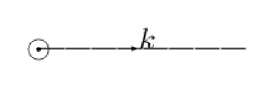
Figure 2: External field of a dilaton with momentum ${\bf k}$.

The relation $\Sigma=aM$ is confirmed classically in the model described by the same Lagrangian in Sec. II DS .

We evaluate the semiclassical amplitudes including the dilatonic sources as well as the dilaton propagators. The dilaton-scalar-scalar vertex (Fig. 3) is given by the expression

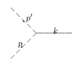
Figure 3: Dilaton-scalar-scalar vertex.

$$V(p^{\prime},p)=-ia\,(p\cdot p^{\prime}+m^{2}\,)\,.$$ (20)

Since the amplitude of one mediating dilaton, which is shown in Fig. 4, is found to be

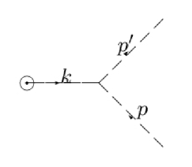
Figure 4: First-order semiclassical amplitude with one dilaton, $i\mathcal{M}_{d}^{(1)}$.

$$i\mathcal{M}^{(1)}_{d}=-a^{2}M\,\frac{1}{{\bf k}^{2}}(EE^{\prime}-{\bf p}\cdot{\bf p}^{\prime}+m^{2})\,.$$ (21)

The lowest-order potential of the dilatonic force can be read from the amplitude as

$$V_{d1}(r)=-\frac{a^{2}Mm}{4\pi r}\left(\frac{m}{E}\right)\approx-\frac{a^{2}Mm}{4\pi r}\left(1-\frac{{\bf p}^{2}}{2m^{2}}\right)\,.$$ (22)

Next, we obtain the vertices contained in the second-order diagrams as the following:

• The dilaton-dilaton-graviton vertex (Fig. 5)

  

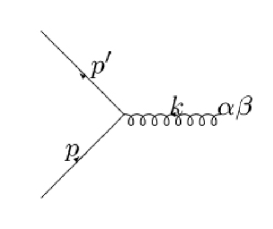
  Figure 5: Dilaton-dilaton-graviton vertex.

  $$V^{\alpha\beta}(p^{\prime},p)=-\frac{i\kappa}{2}[p^{\prime\alpha}p^{\beta}+p^{\prime\beta}p^{\alpha}-\eta^{\alpha\beta}p^{\prime}\cdot p\,]\,.$$ (23)

• The graviton-dilaton-scalar-scalar vertex (Fig. 6)

  

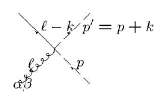
  Figure 6: Graviton-dilaton-scalar-scalar vertex.

  $$V^{\alpha\beta}(p^{\prime},p)=\frac{i\kappa a}{2}[p^{\prime\alpha}p^{\beta}+p^{\prime\beta}p^{\alpha}-\eta^{\alpha\beta}(p^{\prime}\cdot p+m^{2})\,]\,.$$ (24)

• The photon-photon-dilaton vertex (Fig. 7)

  

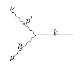
  Figure 7: Photon-photon-dilaton vertex.

  $$V^{\mu,\nu}(p^{\prime},p)=i2a\eta^{\mu\nu}p\cdot p^{\prime}\,.$$ (25)

• The photon-dilaton-scalar-scalar vertex (Fig. 8)

  

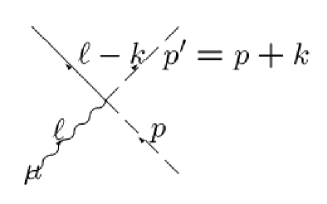
  Figure 8: Photon-dilaton-scalar-scalar vertex.

  $$V^{\mu}(p^{\prime},p)=iaq(p^{\mu}+p^{\prime\mu})\,.$$ (26)

• The dilaton-dilaton-scalar-scalar vertex (Fig. 9)

  

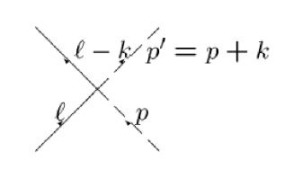
  Figure 9: Dilaton-dilaton-scalar-scalar vertex.

  $$V(p^{\prime},p)=ia^{2}(p\cdot p^{\prime}-m^{2})\,.$$ (27)

Next, we show the amplitudes with diagrams:

• The amplitude for two dilatonic external fields, $i\mathcal{M}^{(2\alpha)}$ (Fig. 10), is given by the expression

  

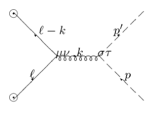
  Figure 10: Amplitude for two dilatonic external fields, $i\mathcal{M}^{(2\alpha)}$.

  $$i\mathcal{M}^{(2\alpha)} = \frac{i}{2}\int^{\Lambda}\frac{d^{3}{\bf l}}{(2\pi)^{3}}\,\phi^{ext}({\bf l})\,\phi^{ext}({\bf l-k})V^{\alpha\beta}(\ell-k,\ell)\,\frac{i\mathcal{P}_{\alpha\beta,\sigma\tau}}{k^{2}}V^{\sigma\tau}(p^{\prime},p)$$ (28)

  $$= -\frac{8\pi Ga^{2}M^{2}}{|{\bf k}|^{2}}\int^{\Lambda}\frac{d^{3}{\bf l}}{(2\pi)^{3}}\,\frac{2({\bf l}-{\bf k})\cdot{\bf p}^{\prime}\,{\bf l}\cdot{\bf p}-{\bf l}\cdot({\bf l}-{\bf k})\frac{1}{2}{\bf k}^{2}}{{\bf l}^{2}({\bf l}-{\bf k})^{2}}$$

  $$= \frac{8\pi Ga^{2}M^{2}}{32|{\bf k}|}\left({\bf p}^{2}-\frac{7}{4}{\bf k}^{2}\right)+{\cal O}(\Lambda)\,.$$

• The amplitude for one dilatonic external field and one gravitational external field, $i\mathcal{M}^{(2\beta)}$ (Fig. 11), is given by the expression below.

  

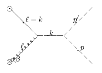
  Figure 11: Amplitude for one dilatonic external field and one gravitational external field, $i\mathcal{M}^{(2\beta)}$.

  $$i\mathcal{M}^{(2\beta)}=i\int\frac{d^{3}{\bf l}}{(2\pi)^{3}}\,h_{\alpha\beta}^{ext}({\bf l})\,\phi^{ext}({\bf l-k})V^{\alpha\beta}(\ell-k,-k)\frac{i}{k^{2}}\,V(p^{\prime},p)=0\,.$$ (29)

• The amplitude for one dilatonic external field and one gravitational external field, $i\mathcal{M}^{(2\gamma)}$ (Fig. 12), is given by the expression

  

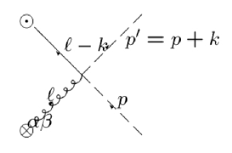
  Figure 12: Amplitude for one dilatonic external field and one gravitational external field, $i\mathcal{M}^{(2\gamma)}$

  $$i\mathcal{M}^{(2\gamma)} = i\int\frac{d^{3}{\bf l}}{(2\pi)^{3}}\,\phi^{ext}({\bf l-k})h_{\alpha\beta}^{ext}({\bf l})V^{\alpha\beta}(p^{\prime},p)$$ (30)

  $$= -\frac{\kappa^{2}a^{2}M^{2}}{8}\int\frac{d^{3}{\bf l}}{(2\pi)^{3}}\frac{1}{{\bf l}^{2}({\bf l}-{\bf k})^{2}}\,(4E^{2}+2m^{2})$$

  $$= -\frac{\kappa^{2}a^{2}M^{2}}{64|{\bf k}|}\,(6m^{2}+4{\bf p}^{2})=-\frac{\pi Ga^{2}M^{2}}{|{\bf k}|}\,(3m^{2}+2{\bf p}^{2})\,.$$

• The amplitude for one dilatonic external field, one gravitational external field and an internal scalar, $i\mathcal{M}^{(2\delta)}$ (Fig. 13), is given by the expression below.

  

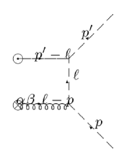
  Figure 13: Amplitude for one dilatonic external field, one gravitational external field and an internal scalar, $i\mathcal{M}^{(2\delta)}$

  $$i\mathcal{M}^{(2\delta)} = 2i\int\frac{d^{3}{\bf l}}{(2\pi)^{3}}\,\phi^{ext}({\bf p^{\prime}-l})V(p^{\prime},\ell)\frac{i}{\ell^{2}-m^{2}+i\epsilon}V^{\alpha\beta}(\ell,p)h_{\alpha\beta}^{ext}({\bf l-p})$$ (31)

  $$= 16\pi GM^{2}a^{2}\,{\int\frac{d^{3}{\bf l}/(2\pi)^{3}\quad(2E^{2}-m^{2})\,(E^{2}-{\bf l}\cdot{\bf p}^{\prime}+m^{2})}{[({\bf p^{\prime}}-{\bf l})^{2}+\mu^{2}][({\bf p}-{\bf l})^{2}+\mu^{2}]({\bf p}^{2}-{\bf l}^{2}+i\epsilon)}}\,.$$

• The amplitude for two electric external fields creating a dilaton external field, $i\mathcal{M}^{(2\epsilon)}$ (Fig. 14), is given as the expression below.

  

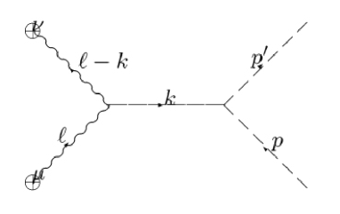
  Figure 14: Amplitude for two electric external fields creating a dilaton external field, $i\mathcal{M}^{(2\epsilon)}$.

  $$i\mathcal{M}^{(2\epsilon)} = \frac{i}{2}\int^{\Lambda}\frac{d^{3}{\bf l}}{(2\pi)^{3}}A_{\mu}^{ext}({\bf l})A_{\nu}^{ext}({\bf l-k})V^{\mu,\nu}(\ell-k,\ell)\frac{i}{k^{2}}V(p^{\prime},p)$$ (32)

  $$= -\frac{a^{2}Q^{2}}{{\bf k}^{2}}\int^{\Lambda}\frac{d^{3}{\bf l}}{(2\pi)^{3}}\,\frac{{\bf l}\cdot({\bf l}-{\bf k})}{{\bf l}^{2}({\bf l}-{\bf k})^{2}}\,(p^{\prime}\cdot p+m^{2})$$

  $$= \frac{a^{2}Q^{2}}{16|{\bf k}|}\left(2m^{2}+\frac{1}{2}{\bf k}^{2}\right)+{\cal O}(\Lambda)=\frac{\pi^{2}a^{2}}{|{\bf k}|}\,\frac{Q^{2}}{(4\pi)^{2}}\left(2m^{2}+\frac{1}{2}{\bf k}^{2}\right)+{\cal O}(\Lambda)\,.$$

• The amplitude for one dilatonic external field and one electric external field, $i\mathcal{M}^{(2\zeta)}$ (Fig. 15), is given as below.

  

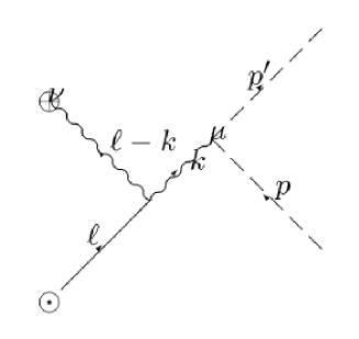
  Figure 15: Amplitude for one dilatonic external field and one electric external field, $i\mathcal{M}^{(2\zeta)}$.

  $$i\mathcal{M}^{(2\zeta)} = i\int\frac{d^{3}{\bf l}}{(2\pi)^{3}}A_{\nu}^{ext}({\bf l-k})\phi^{ext}({\bf l})V^{\mu,\nu}(\ell-k,-k)\frac{-i\eta_{\mu\lambda}}{k^{2}}\,V^{\lambda}(p^{\prime},p)$$ (33)

  $$= \frac{2a^{2}MqQ}{{\bf k}^{2}}\int\frac{d^{3}{\bf l}}{(2\pi)^{3}}\frac{{\bf k}\cdot({\bf l}-{\bf k})}{{\bf l}^{2}({\bf l}-{\bf k})^{2}}\,(p^{0}+p^{\prime 0})$$

  $$= -\frac{a^{2}MqQ}{8|{\bf k}|}\,(2E)=-\frac{\pi a^{2}M}{2}\,\frac{qQ}{4\pi}\,\frac{2E}{|{\bf k}|}\,.$$

• The amplitude for one dilatonic external field and one electric external field, $i\mathcal{M}^{(2\eta)}$ (Fig. 16), is given as

  

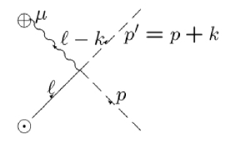
  Figure 16: Amplitude for one dilatonic external field and one electric external field, $i\mathcal{M}^{(2\eta)}$.

  $$i\mathcal{M}^{(2\eta)} = i\int\frac{d^{3}{\bf l}}{(2\pi)^{3}}A_{\mu}^{ext}({\bf l-k})\phi^{ext}({\bf l})V^{\mu}(p^{\prime},p)$$ (34)

  $$= {a^{2}MqQ}\int\frac{d^{3}{\bf l}}{(2\pi)^{3}}\frac{1}{{\bf l}^{2}({\bf l}-{\bf k})^{2}}\,(p^{0}+p^{\prime 0})$$

  $$= \frac{a^{2}MqQ}{8|{\bf k}|}\,(2E)=\frac{\pi a^{2}M}{2}\,\frac{qQ}{4\pi}\,\frac{2E}{|{\bf k}|}\,.$$

• The amplitude for one dilatonic external field, one electric external field and an internal scalar, $i\mathcal{M}^{(2\theta)}$ (Fig. 17), is given as the expression

  

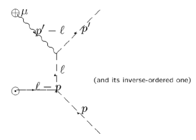
  Figure 17: Amplitude for one dilatonic external field, one electric external field and an internal scalar, $i\mathcal{M}^{(2\theta)}$.

  $$i\mathcal{M}^{(2\theta)} = 2i\int\frac{d^{3}{\bf l}}{(2\pi)^{3}}A_{\mu}^{ext}({\bf p^{\prime}-l})V^{\mu}(p^{\prime},\ell)\frac{i}{\ell^{2}-m^{2}+i\epsilon}V(\ell,p)\phi^{ext}({\bf l-p})$$ (35)

  $$= -2a^{2}MqQ\,{\int\frac{d^{3}{\bf l}/(2\pi)^{3}\qquad(2E)\,(2m^{2}+{\bf p}^{2}-{\bf l}\cdot{\bf p})}{[({\bf p^{\prime}}-{\bf l})^{2}+\mu^{2}][({\bf p}-{\bf l})^{2}+\mu^{2}]({\bf p}^{2}-{\bf l}^{2}+i\epsilon)}}\,.$$

• The amplitude for two dilatonic external fields, $i\mathcal{M}^{(2\iota)}$ (Fig. 18), is given as the expression

  

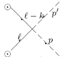
  Figure 18: Amplitude for two dilatonic external fields, $i\mathcal{M}^{(2\iota)}$.

  $$i\mathcal{M}^{(2\iota)} = \frac{i}{2}\int\frac{d^{3}{\bf l}}{(2\pi)^{3}}\phi^{ext}({{\bf l}})\phi^{ext}({\bf{\bf l}-k})V(p^{\prime},p)$$ (36)

  $$= -\frac{a^{4}M^{2}}{2}(p\cdot p^{\prime}-m^{2}){\int\frac{d^{3}{\bf l}}{(2\pi)^{3}}\frac{1}{{\bf l}^{2}({\bf l-k})^{2}}}=-\frac{a^{4}M^{2}}{16|{\bf k}|}\left(\frac{{\bf k}^{2}}{2}\right)\,.$$

• The amplitude for two dilatonic exernal fields and an internal scalar, $i\mathcal{M}^{(2\kappa)}$ (Fig. 19), is given as

  

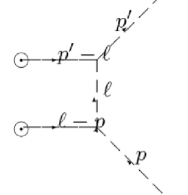
  Figure 19: Amplitude for two dilatonic exernal fields and an internal scalar, $i\mathcal{M}^{(2\kappa)}$.

  $$i\mathcal{M}^{(2\kappa)} = i\int\frac{d^{3}{\bf l}}{(2\pi)^{3}}\phi^{ext}({\bf p^{\prime}-l})V(p^{\prime},\ell)\frac{i}{\ell^{2}-m^{2}+i\epsilon}V(\ell,p)\phi^{ext}({\bf l-p})$$ (37)

  $$= \frac{a^{4}M^{2}}{8\pi^{3}}{\int\frac{d^{3}{\bf l}\quad(E^{2}-{\bf p}\cdot{\bf l}+m^{2})(E^{2}-{\bf p}^{\prime}\cdot{\bf l}+m^{2})}{[({\bf p^{\prime}}-{\bf l})^{2}+\mu^{2}][({\bf p}-{\bf l})^{2}+\mu^{2}]({\bf p}^{2}-{\bf l}^{2}+i\epsilon)}}\,.$$

We define $\mathcal{M}_{d}^{(2~{}total)}$ as the sum of these amplitudes. Consequently, the second-order potential from the diagrams shown above is

$$V_{d2}(r)=\int\frac{d^{3}{\bf k}}{(2\pi)^{3}}e^{i{\bf k}\cdot{\bf r}}\left[\frac{i\mathcal{M}_{d}^{(2~{}total)}}{2E}-\sum_{AB}\int\frac{d^{3}{\bf l}}{(2\pi)^{3}}\frac{\frac{i\mathcal{M}^{(1)}_{A}({\bf p},{\bf l})}{\sqrt{EE^{\prime\prime}/M^{2}}}\frac{i\mathcal{M}^{(1)}_{B}({\bf l},{\bf p})}{\sqrt{E^{\prime\prime}E/M^{2}}}}{E-E^{\prime\prime}}\right]\,,$$ (38)

where the sum is calculated over $(A,B)=(G,d),(d,G),(e,d),(d,e),(d,d)$. Here, the first-order graviton-mediated amplitude is given by Paszko

$$i\mathcal{M}_{G}^{(1)}({\bf p}^{\prime},{\bf p}) = ih^{ext}_{\alpha\beta}({\bf k})V^{\alpha\beta}(p^{\prime},p)$$ (39)

$$= \frac{4\pi GM}{{\bf k}^{2}}(\eta_{\alpha\beta}-2\delta_{\alpha}^{0}\delta_{\beta}^{0})[p^{\prime\alpha}p^{\beta}+p^{\prime\beta}p^{\alpha}-\eta^{\alpha\beta}(p^{\prime}\cdot p-m^{2})]$$

$$= -\frac{4\pi GM}{{\bf k}^{2}}(4EE^{\prime}-2m^{2})\,,$$

where $p=(E,{\bf p})$ and $p^{\prime}=(E^{\prime},{\bf p}^{\prime})$, and the photon-mediated amplitude at the lowest order is Paszko

$$i\mathcal{M}^{(1)}_{e}({\bf p}^{\prime},{\bf p})=iA^{ext}_{\alpha}({\bf k})V^{\alpha}(p^{\prime},p)=\frac{Qq}{{\bf k}^{2}}\,\eta_{\alpha 0}[p^{\alpha}+p^{\prime\alpha}]=\frac{Qq}{{\bf k}^{2}}(E+E^{\prime})\,.$$ (40)

The second-order potential can be computed for ${\bf p}={\bf 0}$, and it is found to be

$$V_{d2}(r)={+\frac{a^{2}Q^{2}m}{2(4\pi)^{2}r^{2}}+\frac{a^{2}M^{2}m}{(4\pi)^{2}r^{2}}-\frac{a^{2}MQq}{(4\pi)^{2}r^{2}}+\frac{a^{4}M^{2}m}{2(4\pi)^{2}r^{2}}}\,.$$ (41)

It is noteworthy that $4\pi G=1$ in this expression.

Finally, we obtain the potential up to $O(1/r^{2})$ for gravitational, electrical, and dilatonic forces. By combining the above result with the potential obtained in Paszko , and accounting for the interchanging symmetry, we obtain the static potential of the two particles labeled $1$ and $2$, that is

$$V_{Ged}(r) = \frac{q_{1}q_{2}-(1+a^{2})m_{1}m_{2}}{4\pi r}+\frac{(1+a^{2})^{2}m_{1}m_{2}(m_{1}+m_{2})}{32\pi^{2}r^{2}}$$ (42)

$$+\frac{(1+a^{2})(m_{1}q_{2}^{2}+m_{2}q_{1}^{2})}{32\pi^{2}r^{2}}-\frac{(1+a^{2})q_{1}q_{2}(m_{1}+m_{2})}{16\pi^{2}r^{2}}\,.$$

It is obvious that if $q_{1}=\sqrt{1+a^{2}}m_{1}$ and $q_{2}=\sqrt{1+a^{2}}m_{2}$, the potential is completely cancelled for any distance. This balance condition is realized in the exact solution in Ref. KSJMP .

IV perihelion precession

Thus far, we have derived the next-to-leading classical interactions in the Einstein-Maxwell system with a dilaton field. It is of theoretical interest to study the perihelion precession if there is a binary of charged dilatonic black holes. The two-body problem of electric charges in general relativity was considered by Barker and O’Connell BO3 . We attempt to apply our result to their formulae for the perihelion precession.

Our previous result leads to the effective Lagrangian for two particles with masses $m_{i}$ and charges $e_{i}$ $(i=1,2)$ (we use $c=1$) as below

$${\cal L}^{\prime}=\frac{1}{2}\mu v^{2}+\frac{G^{\prime}\mu M}{r}+\frac{1}{8}\mu\,k_{1}v^{4}+\frac{3}{2}k_{2}\frac{G^{\prime}\mu Mv^{2}}{r}-\frac{1}{2}k_{3}\frac{{G^{\prime}}^{2}\mu M^{2}}{r^{2}}\,,$$ (43)

where $r\equiv|{\bf r}|=|{\bf r}_{2}-{\bf r}_{1}|$ (the separation), ${\bf v}\equiv{\bf v}_{2}-{\bf v}_{1}$ (the relative velocity), $M\equiv m_{1}+m_{2}$ (the total mass), $\mu\equiv m_{1}m_{2}/M$ (the reduced mass) and

$$G^{\prime}\equiv(1+a^{2})G-\frac{e_{1}e_{2}}{m_{1}m_{2}}\,,$$ (44)

$$k_{1}=1-\frac{3\mu}{M}\,,$$ (45)

$$k_{2}=\frac{1-a^{2}/3}{1+a^{2}}\left(1+\frac{e_{1}e_{2}}{G^{\prime}m_{1}m_{2}}\right)+\frac{2\mu}{3M}\,,$$ (46)

$$k_{3}=1+\frac{\mu}{M}+\frac{e_{1}^{2}m_{2}+e_{2}^{2}m_{1}}{{G^{\prime}}\mu M^{2}}\left(1+\frac{e_{1}e_{2}}{G^{\prime}m_{1}m_{2}}\right)-\left(\frac{e_{1}e_{2}}{G^{\prime}m_{1}m_{2}}\right)^{2}\,.$$ (47)

It is noteworthy that the coordinate transformation according to Barker and O’Connell BO1 ; BO2

$${\bf r}\rightarrow{\bf r}\left(1+\frac{G^{\prime}\mu}{2r}\right)\,,$$ (48)

has been carried out.

The magnitude of precession is given by BO3 ; BO1 , using the above parameters, as follows:

$$\frac{\left(\frac{1}{2}k_{1}+3k_{2}-\frac{1}{2}k_{3}\right)G^{\prime}M\bar{\omega}}{\bar{a}(1-\varepsilon^{2})}\,,$$ (49)

where $\bar{a}$ denotes the semimajor axis, $\varepsilon$ denotes the eccentricity of the orbit, and $\bar{\omega}$ denotes the average orbital angular velocity.

It is interesting to see that only $k_{2}$ depends on the dilaton parameter $a$ if the parameter of the leading force, $G^{\prime}$, is fixed. Therefore, we find that if other conditions are unchanged and only the value of $a$ increases from zero, the precession is reduced.

V Second-order external fields

In this section, we examine the correspondence of the expansion of the exact solution and the external fields obtained perturbatively when the balance condition $Q=\sqrt{1+a^{2}}M$ is satisfied. We propose that there is one charged source at the origin, and the exact solution as given by Eqs. (6) and (9) is expressed using

$$V(r)=1+\frac{(1+a^{2})M}{4\pi r}\,.$$ (50)

The expansions of the metric components of Eq. (6) become

$$g_{00}(r) = V^{-\frac{2}{1+a^{2}}}=1-\frac{2M}{4\pi r}+\frac{(3+a^{2})M^{2}}{(4\pi r)^{2}}+\cdots\,,$$ (51)

$$g_{ij}(r) = -V^{\frac{2}{1+a^{2}}}\delta_{ij}=-\left(1+\frac{2M}{4\pi r}+\frac{(1-a^{2})M^{2}}{(4\pi r)^{2}}+\cdots\right)\delta_{ij}\,.$$ (52)

This can be rewritten as

$$g_{00}(r) = 1-\frac{2M}{4\pi r}+\frac{2M^{2}}{(4\pi r)^{2}}+\frac{Q^{2}}{(4\pi r)^{2}}\cdots\,,$$ (53)

$$g_{ij}(r) = -\left(1+\frac{2M}{4\pi r}+\frac{3M^{2}}{2(4\pi r)^{2}}-\frac{Q^{2}}{2(4\pi r)^{2}}-\frac{a^{2}M^{2}}{2(4\pi r)^{2}}+\cdots\right)\delta_{ij}\,,$$ (54)

by looking at the amplitudes where the scalar probe couples to one graviton Paszko . In other words, these amplitudes are interpreted as the interaction of the perturbed external field and the energy-momentum tensor of the charged dilatonic scalar field Paszko .

Similarly, the expansion of the electric potential becomes

$$A_{0}(r)=\frac{1}{\sqrt{1+a^{2}}}(1-V^{-1})=\frac{\sqrt{1+a^{2}}M}{4\pi r}-\frac{(1+a^{2})^{3/2}M^{2}}{(4\pi r)^{2}}+\cdots\,,$$ (55)

and this expression can be rewritten as

$$A_{0}(r)=\frac{Q}{4\pi r}-\frac{MQ}{(4\pi r)^{2}}-\frac{a^{2}MQ}{(4\pi r)^{2}}+\cdots\,.$$ (56)

This is due to the amplitudes for which the electric charge of the scalar probe appears.

Finally, the expansion of the dilaton field becomes

$$\phi(r)=-\frac{1}{2a}\ln V^{\frac{2a^{2}}{1+a^{2}}}=-\frac{aM}{4\pi r}+\frac{a(1+a^{2})M^{2}}{2(4\pi)^{2}r^{2}}+\cdots\,,$$ (57)

and this expression can be rewritten as

$$\phi(r)=-\frac{aM}{4\pi r}+\frac{aQ^{2}}{2(4\pi)^{2}r^{2}}+\cdots\,.$$ (58)

Eq. (58) is deduced by the amplitudes for which the dilaton coupling to the scalar field is considered.

These considerations are mere confirmations of the exact solution in the second order. However the investigation of this method will be important if we study the perturbative approach from the exact solution, i.e. the solution with the charge-mass relation which slightly deviates from the exact balance condition.

VI $O({\bf p}^{2})$ Hamiltonian and Lagrangian

Thus far, we have omitted the momentum-dependent contribution to the potential in the next-to-leading order. When the leading-order static potential is cancelled or provides a very small contribution, i.e. $Q\approx\sqrt{1+a^{2}}M$, the $O({\bf p}^{2}/r^{2})$ potential cannot be ignored.

The momentum-dependent amplitudes have been shown previously. We do not show the derivation of the potential again; we directly write the result here. The Hamiltonian of the probe with mass $m$ and electric charge $q$ in the system with the fixed mass $M$ at the origin with the charge $Q$, which is the problem considered in the present paper, is given by

$$H = \frac{{\bf p}^{2}}{2m}+\frac{(a^{2}-3)Mm}{2(4\pi)r}\frac{{\bf p}^{2}}{m}$$ (59)

$$+ \frac{m}{2(4\pi)^{2}r^{2}}\left\{\left(1-\frac{a^{2}}{2}\right)\left[Q^{2}-(1+a^{2})M^{2}\right]+2(3-a^{2})M^{2}\right\}\frac{{\bf p}^{2}}{m}+V(r)\,,$$

where

$$V(r)=\frac{Qq-(1+a^{2})Mm}{4\pi r}+\frac{(1+a^{2})^{2}M^{2}m}{2(4\pi)^{2}r^{2}}+\frac{(1+a^{2})Q^{2}m}{2(4\pi)^{2}r^{2}}-\frac{(1+a^{2})MQq}{(4\pi)^{2}r^{2}}\,.$$ (60)

The terms of the order $(1/r)^{3}$ and higher and the order ${\bf p}^{4}$ and higher are neglected.

Subsequently, we obtain the effective Lagrangian for the probe from this Hamiltonian as follows:

$$L = \frac{m{\bf v}^{2}}{2}\left[1+\frac{(a^{2}-3)M}{(4\pi)r}+\frac{1}{(4\pi)^{2}r^{2}}\left\{\left(1-\frac{a^{2}}{2}\right)\left[Q^{2}-(1+a^{2})M^{2}\right]+2(3-a^{2})M^{2}\right\}\right]^{-1}$$ (61)

$$-V(r)$$

$$= \frac{m{\bf v}^{2}}{2}\left[1-\frac{(a^{2}-3)M}{(4\pi)r}-\frac{1}{(4\pi)^{2}r^{2}}\left\{\left(1-\frac{a^{2}}{2}\right)\left[Q^{2}-(1+a^{2})M^{2}\right]+(a^{2}-3)(1-a^{2})M^{2}\right\}\right]$$

$$-V(r)\,,$$

where ${\bf v}={\bf p}/m$ and $O(1/r^{3})$ is dropped consistently.

In the special case with $Q=\sqrt{1+a^{2}}M$ and $q=\sqrt{1+a^{2}}m$, or in other words, when the static balance condition is satisfied, we obtain

$$L=\frac{m{\bf v}^{2}}{2}\left[1+\frac{(3-a^{2})M}{(4\pi)r}+\frac{(3-a^{2})(1-a^{2})M^{2}}{(4\pi)^{2}r^{2}}+O(r^{-3})\right]\,.$$ (62)

The above result agrees with the classical result up to this order moduliS .

The investigation of the system of particles with nearly balanced mass-charge relations by the perturbative method is of considerable interest.

VII Summary and overview

We evaluated the two-body potential of long-range forces coupled with the dilaton field from the perturbative method associated with the Feynman diagrams. Subsequently, we verified the correspondences with the known static exact solutions. Up to the order $O(1/r^{2})$, we showed the cancellation of the static potential under the balance condition, $q_{i}=\sqrt{1+a^{2}}m_{i}\quad(i=1,2)$.

In future, we wish to examine the higher-order contributions involved in the cancellation of classical forces. Further, we wish to study modified theories such as the higher-derivative theories which include dimensionful constants; the investigation of the cancellation of the classical forces are particularly interesting in this case. Further we want to examine the higher-dimensional cases, sources with various spins and other extentions of the perturbative approach.

The calculation of two-body forces on some classical curved backgrounds may describe many-body problems. The perturbative approach will be useful in studying such problems.

The perturbative approach is most suitable in accounting for loop corrections, as in Ref. Faller ; BB . The low-velocity interactions of two or more ‘particles’ are known to be described in terms of the moduli space associated with them if the static forces are cancelled. The structure of the moduli space in the presence of quantum effects is worth studying, particularly for the case with additional fermion fields which can control the loop effect.

References

(1) S. D. Majumdar, Phys. Rev. 72 (1947) 390;
A. Papapetrou, Proc. R. Irish Acad. A51 (1947) 191.
(2) K. Shiraishi, J. Math. Phys. 34 (1993) 1480.
(3)
R. Paszko, arXiv:0801.1835v2 [gr-qc].
See also:
R. Paszko and A. Accioly, Class. Q. Grav. 27 (2010) 145012;
A. Accioly and R. Paszko, Phys. Rev. D78 (2008) 064002;
A. Accioly and R. Paszko, Adv. Stud. Theor. Phys. 3 (2009) 65.
(4) N. E. J. Bjerrum-Bohr, hep-th/0206236v3 (2007).
(5) S. Faller, Phys. Rev. D77 (2008) 124039.
(6) Y.-Z. Chu, Phys. Rev. D79 (2009) 044031.
(7) Y. Degura and K. Shiraishi, Class. Q. Grav. 17 (2000) 4031.
(8) L. D. Landau and E. M. Lifshits, The Classical Theory
of Field, Pergamon Press, Oxford, 1975.
(9) Y. Iwasaki, Prog. Theor. Phys. 46 (1971) 1587.
(10) B. M. Baker and R. F. O’Connell, Lett. Nuovo Cim. 19
(1977) 467.
(11) B. M. Baker and R. F. O’Connell, Phys. Rev. D12
(1975) 329.
(12) B. M. Baker and R. F. O’Connell, J. Math. Phys. 18
(1977) 1818;
ibid.19 (1978) 1231.
(13)
K. Shiraishi, Nucl. Phys. B402 (1993) 399;
Int. J. Mod. Phys. D2 (1993) 59.
(14) K. Shiraishi and T. Maki, Phys. Rev. D53 (1996) 3070.
(15) N. Kan, T. Maki and K. Shiraishi, Phys. Rev. D64
(2001) 104009.