On the classification of the regular components of inner maps.

Abstract.

The topological classification of inner maps on the fully invariant regular components of a wandering set with a special attracting boundary up to the topological conjugacy is defined in terms of distinguishing graph. Two inner maps of the same degree are topologically equivalent on their fully invariant regular components of a certain class if and only if their distinguishing graphs are equivalent.

1. Introduction.

Inner maps were introduced by Stoilov in [2]. Recall that a map is called open if the image of an open set is an open set. A map is called discrete if a preimage of any point is a discrete set (it consists of isolated points). A continuous open discrete map is called inner map. Note that inner maps on compact surfaces have finite number of preimages.

The most noticeable representatives of inner maps are homeomorphisms and holomorphic maps. In fact, an inner map of an oriented surface can be represented as a composition of a non-constant analytical function and a homeomorphism due to Stoilov theorem [2]. It follows the class of inner maps is much wider than holomorphic maps, for example, it includes all homeomorphisms. While dynamics of homeomorphisms, diffeomorphisms and holomorphic maps has been studied deeply in recent times the study of general inner maps with methods of dynamical systems theory just makes its first steps.

The class of inner maps introduced here in definition 2.6 seems exotic at first glance, but this class has such renown representatives as complex polynomials on the Riemannian sphere considered on the basin of attraction to infinity due to the Böttcher theorem [1]. Classification of dynamics on the attraction basin is done up to the topological conjugacy.

Theorem 1.1 (Main theorem).

Restrictions of inner maps $f$, $g$ on the fully invariant regular components of wandering set with a fully invariant pseudolinear attracting isolated connected component satisfying definitions 2.6 and 2.7 are topologically equivalent if and only if they have the same degree and the corresponding distinguishing graphs are equivalent.

2. Preliminary information.

Let $f\colon M\to M$ be an inner map of a compact surface M. Denote by $O^{+}(x)=\{f^{n}(x)|n\geq 0\}$ a forward trajectory of $x$, $O^{-}(x)=\{f^{-n}(x)|n\geq 0\}$ a backward trajectory of $x$, and $O(x)=\{f^{-n}\circ f^{m}(x)|n,m\geq 0\}$ a full trajectory of $x$. Let us call the set $O^{\perp}(x)=\{f^{-n}\circ f^{n}(x)|n\geq 0\}$ a neutral section of trajectory.

Definition 2.1.

A point $x$ is called wandering if there exists an open set $U(x)$ such that $\forall n\in\mathbb{Z},n\not=0$ $f^{n}\left(U(x)\right)\cap U(x)=\varnothing$.

A point which is not wandering is called nonwandering. The set of nonwandering points of $f$ is denoted by $\Omega(f)$. Denote by $B_{\varepsilon}(X)$ the $\varepsilon$-neighborhood of X.

Definition 2.2.

A point $x$ is said to be $\omega$-regular wandering if it is wandering and $\forall\varepsilon>0$ $\exists\delta>0$, $\exists N>0$: $\forall n>N$ $f^{n}\left(B_{\delta}(x)\right)\subset B_{\varepsilon}(\Omega)$.

Definition 2.3.

A point $x$ is called $\alpha$-regular wandering if it is wandering and $\forall\varepsilon>0$ $\exists\delta>0$, $\exists N>0$: $\forall n>N$ $f^{-n}\left(B_{\delta}(x)\right)\subset B_{\varepsilon}(\Omega)$.

A point which is both $\alpha$-regular and $\omega$-regular is called regular. A connected component of the set of regular wandering points is called a regular component of wandering set. A component $U$ is called periodic if there exists n such that $f^{n}(U)=U$. When $n=1$ a periodic component $U$ is called invariant. Also, when $f^{-1}(U)=U$, an invariant component is called fully invariant. Fully invariant components are important because study of periodic components can be essentially reduced to the study of fully invariant components.

Definition 2.4.

An isolated connected component $\partial_{0}$ of the boundary $\partial U$ of a fully invariant regular component $U$ of wandering set is attracting if it has a strictly invariant neighborhood $V(\partial_{0})$ (a neighborhood such that $\overline{f(V)}\subset V$).

Definition 2.5.

An attracting isolated connected component $\partial_{0}$ of the boundary $\partial U$ of a fully invariant regular component $U$ of wandering set is radially pseudolinear if it has strictly invariant neighborhood $V(\partial_{0})$ such that there exists a regular compact invariant foliation of $U\cap V$. Equivalently, it can be defined as a foliation by a function $\Phi\colon V\to[0,1]$ such that $\Phi$ is regular in $U\cap V$ and $\Phi(f(x))=\lambda\Phi(x)$, $\lambda>0$.

Definition 2.6.

A radially pseudolinear attracting isolated connected component $\partial_{0}$ of the boundary $\partial U$ of a fully invariant regular component $U$ of wandering set is pseudolinear if $\forall x\in U\cap V$ $O^{\perp}(x)$ is dense in the foliation fiber of $x$.

Definition 2.7 (Genericity condition.).

The genericity condition is a condition such that every fiber of the $\Phi$ foliation has no more than one image of critical point.

Definition 2.8.

A closed neighborhood $Q\subset U$ is called fundamental neighborhood of $U$ if

1. it is closure of its interior;

2. $\forall x\in U$ $O(x)\cap Q\not=\varnothing$
   ($Q$ contains a representative of every full trajectory in $U$);

3. if $x\in Q,x\not\in\partial Q$ then $f(x)\not\in Q$.

Definition 2.9.

Fundamental neighborhood $Q$ is called saturated if for every $x\in Q$ $Q$ contains $O^{\perp}(x)$.

Lemma 2.1.

Fundamental neighborhoods in the attracting neighborhood from the definition 2.5 are homeomorphic to the ring.

Proof.

Note that the attracting component of boundary is isolated, it means that the strictly invariant neighborhood is connected, so the foliation does not have holes. Otherwise other components of boundary will be attracted to the attracting component, which will contradict isolatedness.

Since the boundary of strictly invariant neighborhood should also belong to the foliation and the foliation is regular compact then all fibers are homeomorphic to the circle. Due to the regularity of the foliation, the neighborhood does not contain critical points or their preimages. Hence, the map between a fundamental neighborhood and its image is a regular covering. But a Mëbius string can only cover a Mëbius string, handles can only cover handles, and if there exists any, there should be infinitely many of them, as fundamental neighborhood has infinitely many images. It contradicts to compactness. Since a fundamental neighborhood can’t have a handle or a Mëbius string, therefore $Q$ is homeomorphic to the ring. ∎

Remark 2.1.

In the theorem1.1 we consider a fully invariant pseudolinear attracting isolated connected component of the boundary. Because it is fully invariant, then equiscalar lines of the function $\Phi$ from the definition 2.5 in the fundamental neighborhood $Q$ from the lemma 2.1 consist of a single circle with the property that for its each point the circle also contains the whole set $O^{\perp}$ of that point.

Lemma 2.2.

A fully invariant regular component $U$ of wandering set with a radially pseudolinear attracting isolated connected component is either homeomorphic to the ring (have the only other component of the boundary) in case it has no critical points or it has infinite number of boundary components.

a)  b)

Figure 1. a) Regular foliation b) foliation at the critical trajectory of degree 3.

Proof.

By lemma 2.1 all the fundamental neighborhoods in the attracting neighborhood from the definition 2.5 are homeomorphic to the ring. In absence of critical points all the fundamental neighborhoods are homeomorphic, hence the whole regular component is homeomorphic to the ring.

In case when there are critical trajectories there are finite number of them due to compactness. By definition 2.5, the whole fully invariant neighborhood $U\cap V$ of the regular component $U$ does not contain critical points. Choose a fundamental neighborhood $Q\subset U\cap V$. Note that $Q$ is homeomorphic to the ring according to the lemma 2.1.

Consider the first preimage of $Q$ that contain a critical point. It is enough to consider a single critical point case, the deduction in the case of multiple critical points is the same.

According to the Stoilov’s “lemma on simple curve” [2], a critical point should distort the foliation causing the fibers to intersect. In the image of critical point the foliation is regular, as on figure 1a, while in the critical point $p$ and its preimages there is an intersection of $n$ fibers, where $n$ is the degree of $p$. This situation is shown on figure 1b.

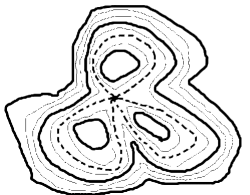
a) b)

Figure 2. a) Wandering critical point. b) Numeration on $O^{\perp}(x)$.

Since fibers have dimension 1, they locally divide the surface $M$. As shown in the proof of lemma 2.1, the fibers of the fundamental neighborhood $Q$ are circles. Then, the critical preimage of a circle is a bouquet of circles. Every circle of the bouquet divide the regular component $U$. Thus, preimage of $Q$ has $n+1$ components of boundary. This situation is shown on the picture 2a). The set $\cup_{k=-1}^{\infty}f^{k}(Q)$ also has $n+1$ components of boundary because the rest of the fundamental neighborhoods $f^{k}(Q)$, $k\geq 0$, are homeomorphic to the ring. The further preimages of $Q$ are disjoint union of components of connectedness each of them is either homeomorphic to $f^{-1}(Q)$ or cover it. It means that $\cup_{k=-2}^{\infty}f^{k}(Q)$ will have not less than $n^{2}+1$ components of boundary, $\cup_{k=-3}^{\infty}f^{k}(Q)$ will have not less than $n^{3}+1$ components of boundary, and so on. As a consequence, $U=\cup_{k=-\infty}^{\infty}f^{k}(Q)$ should have infinitely many components of boundary. If there are other critical points, the number of boundary components just will grow faster, so the same reasoning is applicable too. ∎

2.1. Coordinates on a fundamental neighborhood.

Consider a saturated fundamental neighborhood $Q$ that is homeomorphic to the ring as in lemma 2.1. Note that the boundary of $Q$ consists of foliation fibers. Choose an orientation on $Q$. As the points of $O^{\perp}(x)$ for a point $x\in Q$ belongs to the same homeomorphic to a circle fiber (see remark 2.1), they are naturally cyclically ordered. Assign a point $y\in f^{-n}\circ f^{n}(x)\subset O^{\perp}(x)$ a pair $\{k,m^{n}\}$, where $m$ is a degree of covering $Q$ by $f$, $n$ is the iteration number as in $f^{-n}\circ f^{n}$, the number $k$ is a cyclic order of $y$ among other points of the preimage $(f^{-n}\circ f^{n})(x)$ according to the orientation of the fiber. Note that $0\leq k<m^{n}$, $0$ is for $x$, $1$ is for the first another preimage of $x$ under $f^{-n}\circ f^{n}$ in the direction of orientation. Let as write those pairs as fractions, for example, the pair $\{k,m^{n}\}$ is written as fraction $\frac{k}{m^{n}}$. Assign the point $x$ a pair $\frac{0}{1}$. An example of the numeration for the degree $2$ is shown on the figure 2b). Note that pairs that denote the same numeric fraction (like $\frac{1}{2}$ and $\frac{2}{4}$) belong to the same point.

A fundamental neighborhood $Q$ already has one family of coordinate lines due to the foliation. The other family can be built as follows. Choose a point $x\in\partial Q$ such that $f(x)\in\partial Q$. Then $x$ and $f(x)$ are on different connected components of $\partial Q$ which are fibers of the foliation. Connect $x$ and $f(x)$ with a “transversal” to the foliation jordan curve $\gamma$ that intersects each fiber in a single point. Then the images $f^{-n}\circ f^{n}(\gamma)$ will not intersect with each other because for every $x\in\gamma$ the set $O^{\perp}(x)$ belongs to the fiber of $x$, but $\gamma$ intersect fibers in a unique point. Then the set $O^{\perp}(\gamma)=\cup_{n=0}^{\infty}f^{-n}\circ f^{n}(\gamma)$ will yield an everywhere dense family of curves according to the definition 2.6 of pseudolinearity. Note that each image of the curve $\gamma$ can be assigned a pair $\frac{k}{m^{n}}$ in the same way as for the images of a point.

This lamination $O^{\perp}(\gamma)$ can be extended to foliation by continuity. For a point $x\in Q\setminus O^{\perp}(\gamma)$ define $\mu(x)=\cap_{n\geq 0}\Delta_{n}(x)$, where $\Delta_{n}(x)$ is closure of connected component of the set $Q\setminus f^{-n}\circ f^{n}(\gamma)$ that contains the point $x$. As an intersection of closed sets the set $\mu(x)$ has non-empty intersection with every equiscalar line of foliation of $Q$. Show that $\mu(x)$ intersect each fiber in a unique point. Suppose on the contrary that there exists a fiber $\nu$ such that it is intersected by $\mu(x)$ in 2 points $y_{1}$ and $y_{2}$. Denote by $z$ a point of intersection $\nu$ and $\gamma$. Then by construction the whole segment $[y_{1},y_{2}]$ of the fiber $\nu$ belongs to $\mu(x)$. But it contradicts the fact that $O^{\perp}(z)$ is everywhere dense in $\nu$ according to definition 2.6. Hence $\mu(x)$ intersects each equiscalar line in a unique point. By construction, $\mu(x)$ continuously depends on equiscalar lines foliation as $\mu(x)$ is majorated by images of $\gamma$. As a consequence, it is also a jordan curve.

Thus, we constructed two families of curves on $Q$ such that their fibers intersect each other in a single point. Note that the foliation on equiscalar lines is a topological invariant of $f$, while the second foliation is arbitrary up to choice of $\gamma$.

2.2. Global Coordinates.

Constructed above two families of curves on $Q$ generate two families of curves on the whole regular component $U$ under the action of $f$ and $f^{-1}$. Let us call a foliation of $\Phi$ the neutral foliation and the foliation induced by $\gamma$ the timeline foliation. By construction

• they are invariant under the action of $f$;

• they are regular except in critical points and their preimages.

Remark 2.2.

$f$ acts as homeomorphism on non-critical fibers of the timeline foliation.

Proof.

It follows from the fact that a fiber of timeline foliation intersects every fiber of neutral foliation, and, hence, intersects each set $O^{\perp}$ in no more then one point. ∎

Note that neutral coordinates on neutral fibers are defined on the dense set $O^{\perp}(\gamma)$ and are continuous by construction. They can be extended by continuity to a function $\nu\colon Q\to S^{1}=[0,1]\mod 1$.

By choosing a function $\tau^{\prime}\colon\gamma\to[0,1]$ and extending it to constant on the neutral fibers function $\tau^{\prime}\colon Q\to[0,1]$ every point $p\in Q$ can be assigned unique coordinates $(x=\nu(p),y=\tau(p))$, $x\in[0,1)$, $y\in[0,1]$.

If there are no critical points those coordinates can be extended to the coordinates on $U$ $(x,y)$, $x\in[0,1)$, $y\in\mathbb{R}$ by the following rule. For a point $p\in U$ a neutral coordinate $x$ is determined by the neutral coordinate of continuation of its timeline fiber, and the timeline coordinate $y$ is determined by equation $y=y^{\prime}+n$, where $y^{\prime}=\tau(f^{n}(p))$ is timeline coordinate of $f^{n}(p)\in Q$. Call them $\gamma$-coordinates.

Lemma 2.3.

Two regular components $U_{1}$ and $U_{2}$ of wandering sets of inner maps $f$ and $g$ of the same degree with a pseudolinear attracting isolated connected components of the boundary without critical points are topologically conjugate.

Proof.

Choose arbitrarily saturated fundamental neighborhoods $Q_{1}$ and $Q_{2}$ of $U_{1}$ and $U_{2}$ and transversal curves $\gamma_{1}\subset Q_{1}$ and $\gamma_{2}\subset Q_{2}$ to neutral foliations in $Q_{1}$ and $Q_{2}$. Construction above extends them to the two pairs of foliations in $Q_{1}$ and $Q_{2}$.

Choose a homeomorphism $h^{\prime}_{\gamma}\colon\gamma_{1}\to\gamma_{2}$. Continue $h^{\prime}_{\gamma}$ over the timeline foliation using maps $(g^{-k}\circ g^{l})^{-1}\circ h^{\prime}_{\gamma}\circ f^{-k}\circ f^{l}$, $k,l\geq 0$. Note that branches of those maps are homeomorphisms when restricted on a single fiber (see remark 2.2) so they have inverse homeomorphisms which are denoted here as $(g^{-k}\circ g^{l})^{-1}$. Denote the obtained map by $\hat{h}_{\gamma}$. Since $f$ and $g$ preserve their neutral foliations, $\hat{h}_{\gamma}$ maps points that belong to the same fiber of the neutral foliation of $f$ to the points on the same fiber of the neutral foliation of $g$. Because $f$ and $g$ have the same map degree they act the same way on the points that have the same neutral coordinates. It means that $\hat{h}_{\gamma}$ induces not only mapping of timeline foliations, but also a mapping of neutral foliations.

It can be extended by continuity to a bijection $h_{\gamma}$ between $U_{1}$ and $U_{2}$. This bijection is continuous, since foliations are continuous. Also $h_{\gamma}$ is an open map because in every point it maps its base of topology built from foliation boxes to the corresponding base of topology generated by foliations in the image. It shows that $h_{\gamma}$ is a homeomorphism. By construction, $h_{\gamma}\circ f=g\circ h_{\gamma}$, it means that $f$ and $g$ are topologically conjugate.

Note that if one choose $h^{\prime}_{\gamma}$ to map identical timeline $\gamma$-coordinates on $U_{1}$ and $U_{2}$ then $h_{\gamma}$ in corresponding $\gamma$-coordinates on $U_{1}$ and $U_{2}$ will be nothing but $\mathop{\mathrm{Id}}\nolimits$. ∎

3. Distinguishing graph.

As shown in lemma 2.3 in case when there are no critical points the topological classification is simple. The only essential invariant is the map degree.

In case when there are critical points the symmetry of points breaks. Topological conjugacy distinguish among critical and non-critical points, their preimages and foliation fibers. To deal with this extra topological invariants we need to build a distinguishing graph which is technically a compact encoding of some labelled Konrod-Reeb graph of a specially chosen part of the foliation function.

Choose the fundamental neighborhood to be the neighborhood between the boundary of the first and second images of the first critical level of the invariant neutral foliation. Note that due to the choice of the fundamental neighborhood and the genericity condition from definition 2.7 any fiber of the neutral foliation in the chosen fundamental neighborhood has no more than one image of a critical point and there are finitely many fibers that have an image of a critical point. Choose the line $\gamma$ that generates the timeline foliation to intersect each fiber with a critical point in that critical point, including the boundary fibers of the fundamental neighborhood. In absence of critical points the points of regular component can be uniquely identified by a pair of coordinates on its timeline and neutral fibers ($\gamma$-coordinates introduced above). But the critical points make foliation singular so that lines of timeline foliation intersect in critical points and their preimages. Also preimages of the fundamental neighborhood divide onto components such that internals of those components are mutually disconnected. It follows that timeline $\gamma$-coordinates can be defined the same way as in absence of critical points, but neutral $\gamma$-coordinates can’t.

In that case introduce neutral $\gamma$-coordinates that are local to a component of a preimage of the fundamental neighborhood $Q$. Consider the fiber $\widehat{\gamma}$ of timeline foliation that contains the original curve $\gamma\in Q$. This fiber branches in critical points and their preimages simultaneously together with dividing of preimages of the fundamental neighborhood $Q$ onto components so than there is a unique branch of the singular fiber $\widehat{\gamma}$ that goes into internals of each component. Now construct neutral coordinates for every component using this branch of $\widehat{\gamma}$ as local origin $\frac{0}{1}$. At that points at the component boundary might get different neutral coordinates from components the point borders with. To avoid the ambiguity let us always assume that the component of the boundary further from attractor should belong to the component and inherit its numeration. From that the critical points and their preimages will get the neutral coordinate $\frac{0}{1}$.

Also, those coordinates are not unique: there are finitely many components having the same coordinates. To avoid this ambiguity component of a preimage should be counted for every $n$ such that every point of $U$ could be identified with a triplet $(x,y,C)$, where $x$ is a local neutral coordinate, $y$ is a global timeline coordinate, and $C$ is a component number.

To enumerate the components choose an orientation on the boundary of the original fundamental neighborhood $Q$. Since the regular component is oriented, this orientation induces an orientation on the preimages of the boundary. Starting from a point on the original curve $\gamma$ and move on the singular fiber $\widehat{\gamma}$ there is a unique shortest path to walk over all components of preimage of the border of $Q$ moving on the preimages according to the orientation and moving according to the orientation from one component to another on $\widehat{\gamma}$. That path cyclically orders components. Number them according to that order so the first component met on that path will get the number 1. This numeration is related to the first critical point.

The other critical points further subdivide some of those components, in such a way that those subcomponents share the same regular component of the singular neutral foliation of the previous critical point. so in that case it is natural to create a compound number by assigning such a component the sequence of numbers each related to the critical neutral fiber of corresponding critical point. Call the obtained compound number $C=\{k_{1},\dots,k_{l}\}$ a component number.

By construction critical points are identified by a triplet $(\frac{0}{1},n+y^{\prime},C)$, which does not depend on the choice of $\gamma$. It only has compound component number depending on choice of orientation and timeline coordinate $y$ having invariant integer part $n$ and a fraction part $y^{\prime}$ depending on the choice of the timeline function $\tau$. However, the relative order of images and preimages of critical neutral fibers does not depend on the choice of $\tau$.

Project the critical points on the semi-interval $[0,1)$ using their fractional parts $y^{\prime}$ of their timeline coordinates and label them with pairs $(d,n,C\overline{C})$, where $d$ is a local degree of the critical point, $C\overline{C}$ is an unordered pair of component numbers with different choices of orientation in $Q$. Note that the first critical point gets by construction the label $(...,0,\{1\}\{1\})$.

Definition 3.1.

Two labels are equal if their components are equal: the first and second components are equal as numbers, the third components are equal as unordered pairs of vectors.

Definition 3.2.

Call the semi-interval $[0,1)$ either without labelled points or with labelled points such that $0$ is labelled and $0$’s label looks like $(...,0,\{1\}\{1\})$ a distinguishing graph.

Definition 3.3.

Two distinguishing graphs are equivalent if there exists a homeomorphism of the semi-interval $[0,1)$ such that the labels of images and preimages are equal.

Proof of the main theorem..

The proof is similar to the proof of the lemma 2.3, except we have not global but local coordinate families in each component of preimage of the fundamental neighborhood that are built is section 3. By definition the equivalence of the distinguishing graphs guarantees one-to-one correspondence between adjacent components. As in lemma  2.3, it follows that a map written in that coordinates as $\mathop{\mathrm{Id}}\nolimits$ is the desired homeomorphism. ∎

References

- [1] Milnor J. Dynamics in One Complex Variable. Introductory lectures. // Braunschweig. –1999.
- [2] Stoïlow S. Leçon sur les principes topologiques de la theorie des fonctions analytiques. // Paris. –1938.
- [3] Trokhymchuk Yu. Yu. Differentiating, inner mappings and analyticity criteria. // Proceedings of Institute of Math., vol. 70. Kiev. – 2008. 538 p.