Self-induced tunable transparency in layered superconductors

Abstract

We predict a novel nonlinear electromagnetic phenomenon in layered superconducting slabs irradiated from one side by an electromagnetic plane wave. We show that the reflectance and transmittance of the slab can vary over a wide range, from nearly zero to one, when changing the incident wave amplitude. Thus changing the amplitude of the incident wave can induce either the total transmission or reflection of the incident wave. In addition, the dependence of the superconductor transmittance on the incident wave amplitude has an unusual hysteretic behavior with jumps. This remarkable nonlinear effect (self-induced transparency) can be observed even at small amplitudes, when the wave frequency $\omega$ is close to the Josephson plasma frequency $\omega_{J}$.

I Introduction.

The recent growing interest in the unusual electrodynamic properties of layered superconductors (see, e.g., the very recent review Ref. Thz-rev-2008-July, ) is due to their possible applications, including terahertz imaging, astronomy, spectroscopy, chemical and biological identification. The experiments for the $\mathbf{c}$-axis conductivity in high-$T_{c}$ $\rm Bi_{2}Sr_{2}CaCu_{2}O_{8+\delta}$ single crystals justify the use of a model in which the very thin superconducting CuO₂ layers are coupled by the intrinsic Josephson effect through the thicker dielectric layers Thz-rev-2008-July ; Kl-Mu ; Kl-Mu2 ; bran ; plasma . Thus, a very specific type of plasma (the so-called, Josephson plasma) is formed in layered superconductors. The current-carrying capability of this plasma is strongly anisotropic, not only in the absolute values of the current density. Even the physical nature of the currents along and across layers is quite different: the current along the layers is the same as in usual bulk superconductors, whereas the current across the layers originates from the Josephson effect. This Josephson current flowing along the $\mathbf{c}$-axis couples with the electromagnetic field inside the insulating dielectric layers, causing a specific kind of elementary excitations called Josephson plasma waves (JPWs) (see, e.g., Ref. Thz-rev-2008-July, and references therein). Therefore, the layered structure of superconductors favors the propagation of electromagnetic waves through the layers.

The electrodynamics of layered superconductors is described by nonlinear coupled sine-Gordon equations SG-coupled ; SG2 ; SG3 ; SG4 ; SG5 ; Thz-rev-2008-July . This nonlinearity originates from the nonlinear relation $J\propto\sin\varphi$ between the Josephson interlayer current $J$ and the gauge-invariant interlayer phase difference $\varphi$ of the order parameter. As a result of the nonlinearity, a number of nontrivial nonlinear phenomena nl1 ; nl2 ; nl3 ; nl4 ; nl5 (such as slowing down of light, self-focusing effects, the pumping of weaker waves by stronger ones, etc.) have been predicted for layered superconductors. The nonlinearity plays a crucial role in the JPWs propagation, even for small wave amplitudes, $|\varphi|\ll 1$, when $\sin\varphi$ can be expanded into a series as $(\varphi-\varphi^{3}/6)$, for frequencies close to the Josephson plasma frequency.

In this paper, we predict a novel and unusual strongly nonlinear phenomenon. The reflectance and transmittance of a superconducting slab being exposed to an incident wave from one of its sides depend not only on the wave frequency and the incident angle, but also on the wave amplitude. If the frequency $\omega$ of irradiation is close to the Josephson plasma frequency $\omega_{J}$, the transmittance of the slab can vary over a wide range, from nearly zero to one. Therefore, a slab of fixed thickness can be absolutely transparent (when neglecting dissipation) for waves of definite amplitudes, and nearly totally reflecting for other amplitudes. This unusual property can be described as self-induced tunable transparency. Moreover, the dependence of the transmittance on the wave amplitude shows hysteretic behavior with jumps. Tunable electromagnetically induced transparency is also now being studied in various contexts, including superconducting circuits and other lambda-type atoms (see, e.g., Refs. tt1, ; tt2, ).

The large sensitivity of the slab transmittance to the wave amplitude can be explained using a very clear physical consideration. Let us consider a wave frequency $\omega$ which is slightly smaller than the Josephson plasma frequency $\omega_{J}$. In this case, linear JPWs cannot propagate in the layered superconductor (see, e.g., Ref. Thz-rev-2008-July, ). So, the slab is opaque for waves with small amplitudes, and the transmittance is exponentially small due to the skin effect. According to Refs. nl1, ; nl2, ; nl3, , the nonlinearity results in an effective decrease of the Josephson plasma frequency and, thus, nonlinear JPWs with high-enough amplitudes can propagate in the superconductor. Moreover, changing the amplitude of the incident wave one can attain the conditions when the slab thickness equals an integer number of half-wavelengths. Under such conditions, the slab becomes transparent, with its transmittance equal to one.

The paper is organized as follows. In section II, we discuss the geometry of the problem and present the main equations for the electromagnetic fields both in the vacuum and in the slab of layered superconductor. In section III, we express the transmittance $T$ in terms of the amplitude of the incident wave and analyze this dependence in two cases: when the frequency $\omega$ of the incident wave is either larger or smaller than the Josephson plasma frequency $\omega_{J}$. In both cases, we study the unusual hysteretic features of this dependence. The results of numerical simulations support our theoretical predictions.

II Spatial distribution of the electromagnetic field

II.1 Geometry of the problem

We study a slab of layered superconductor of thickness $D$ (see Fig. 1). Superconducting layers of thickness $s$ are interlayed by insulators of much larger thickness $d$ ($s\ll d$). We assume the number of layers to be large, allowing the use of the continuum limit, and not to consider the spatial distribution of the electromagnetic field inside each layer. The coordinate system is chosen in such a way that the crystallographic $\mathbf{ab}$-plane coincides with the $xy$-plane, and the $\mathbf{c}$-axis is along the $z$-axis. The plane $z=0$ corresponds to the lower surface of the slab.

A monochromatic electromagnetic plane wave of frequency $\omega$ is incident on the upper surface of the slab, and it is partly reflected and partly transmitted through the slab. We consider the incident wave of the transverse magnetic polarization, when the magnetic field is parallel to the surface of the slab,

$${\vec{E}}=\{E_{x},0,E_{z}\},\qquad{\vec{H}}=\{0,H,0\}.$$ (1)

The incident angle $\theta$ is considered to be not close to zero, so that both components $k_{x}$ and $k_{z}$ of the wave-vector $\textbf{k}_{i}$ are of the order of $\omega/c$.

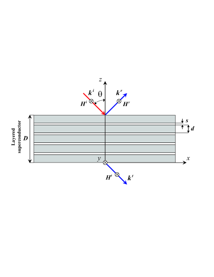
Figure 1: (Color online) Geometry of the problem. A slab of layered superconductor is irradiated from the upper side by a $p$-polarized electromagnetic wave.

II.2 Electromagnetic field in the vacuum

The magnetic field $H^{u}$ in the upper vacuum semispace ($z>D$) can be represented as a sum of the incident and reflected waves with amplitudes $H_{0}$ and $H_{r}$, respectively. The field $H^{l}$ in the vacuum semispace below the sample ($z<0$) is the transmitted wave with amplitude $H_{t}$. The upper ($H^{u}$) and lower ($H^{l}$) fields and can be written in the following form,

$$H^{u}=H_{0}\cos[k_{x}x-\omega t-k_{z}(z-D)]$$

$$+H_{r}\cos[k_{x}x-\omega t+k_{z}(z-D)+\alpha],$$ (2)

$$H^{l}=H_{t}\cos(k_{x}x-\omega t-k_{z}z+\beta).$$ (3)

Here

$$k_{x}=\frac{\omega}{c}\sin\theta,\quad k_{z}=\frac{\omega}{c}\cos\theta,$$ (4)

are the components of the wave-vector $\textbf{k}_{i}$ of the incident wave, $\alpha$ and $\beta$ are the phase shifts of the reflected and transmitted waves. Using Maxwell equations one can derive the electric field components in the vacuum:

$$E_{x}^{u}=-H_{0}\cos\theta\cos[k_{x}x-\omega t-k_{z}(z-D)]$$

$$+H_{r}\cos\theta\cos[k_{x}x-\omega t+k_{z}(z-D)+\alpha],$$ (5)

$$E_{z}^{u}=-H_{0}\sin\theta\cos[k_{x}x-\omega t-k_{z}(z-D)]$$

$$-H_{r}\sin\theta\cos[k_{x}x-\omega t+k_{z}(z-D)+\alpha],$$ (6)

$$E_{x}^{l}=-H_{t}\cos\theta\cos(k_{x}x-\omega t-k_{z}z+\beta),$$ (7)

$$E_{z}^{l}=-H_{t}\sin\theta\cos(k_{x}x-\omega t-k_{z}z+\beta).$$ (8)

II.3 Electromagnetic field in the layered superconductor

The electromagnetic field inside a layered superconductor slab is determined by the distribution of the gauge-invariant phase difference $\varphi(x,z,t)$ of the order parameter between the layers (see, e.g., Ref. Thz-rev-2008-July, ),

$$\frac{\partial H^{s}}{\partial x}=\frac{{\cal H}_{0}}{\lambda_{c}}\Big{(}\frac{1}{\omega_{J}^{2}}\frac{\partial^{2}\varphi}{\partial t^{2}}+\sin\varphi\Big{)},$$

$$E^{s}_{x}=-\frac{\lambda^{2}_{ab}}{c}\frac{\partial^{2}H^{s}}{\partial z\partial t},\qquad E_{z}^{s}=\frac{{\cal H}_{0}\lambda_{c}}{c}\frac{\partial\varphi}{\partial t}.$$ (9)

Here ${\cal H}_{0}=\Phi_{0}/2\pi d\lambda_{c}$, $\Phi_{0}=\pi c\hbar/e$ is the magnetic flux quantum, $\lambda_{ab}$ and $\lambda_{c}=c/\omega_{J}\epsilon^{1/2}$ are the London penetration depths across and along the layers, respectively. The Josephson plasma frequency is defined as

$$\omega_{J}=\sqrt{\frac{8\pi edJ_{c}}{\hbar\epsilon}},$$ (10)

where $J_{c}$ is the critical value of the Josephson current density, $\epsilon$ is the permittivity of the dielectric layers in the slab. We omit the relaxation terms because, at low temperatures, they do not play an essential role in the phenomena considered here.

The phase difference $\varphi$ obeys a set of coupled sine-Gordon equations, that, in the continuous limit, takes on the following form (see, e.g., Ref. Thz-rev-2008-July, and references therein):

$$\left(1-\lambda_{ab}^{2}\frac{\partial^{2}}{\partial z^{2}}\right)\left[\frac{1}{\omega^{2}_{J}}\frac{\partial^{2}\varphi}{\partial t^{2}}+\sin\varphi\right]-\lambda_{c}^{2}\frac{\partial^{2}\varphi}{\partial x^{2}}=0.$$ (11)

In this paper, we study the case of weak nonlinearity: when the Josephson current density $J_{c}\sin\varphi$ can be expanded as a series for small $\varphi$, up to the third order, $J_{c}\sin\varphi\approx J_{c}(\varphi-\varphi^{3}/6)$. We consider frequencies $\omega$ close to $\omega_{J}$ and introduce a dimensionless frequency,

$$\Omega=\frac{\omega}{\omega_{J}},$$

close to one. In this case, in spite of the weakness of the nonlinearity in Eq. (11), the linear terms nearly cancel each other, and the term $\varphi^{3}$ plays a crucial role in this problem. Moreover, when the frequency $\omega$ is close to the Josephson plasma frequency $\omega_{J}$, one can neglect the generation of higher harmonics nl1 ; nl3 .

It should be also noted that the nonlinearity provides an effective decrease of $\omega_{J}$. Indeed, the expression in the square brackets in Eq. (11) can be presented in the form $[(\omega^{\rm eff}_{J})^{-2}\partial^{2}\varphi/\partial t^{2}+\varphi]$, where

$$\omega^{\rm eff}_{J}\approx\omega_{J}\Big{(}1-\dfrac{\varphi^{2}}{12}\Big{)}.$$

For not very small $\varphi$, the frequency of the incident wave can be greater than the effective Josephson plasma frequency $\omega^{\rm eff}_{J}$ and, therefore, the nonlinear Josephson plasma waves can propagate across the superconducting layers.

The $z$-component of the electric field induces a charge in the superconducting layers when the charge compressibility is finite. This results in an additional interlayer coupling (so-called, capacitive coupling). Such a coupling significantly affects the properties of the longitudinal Josephson plasma waves with wave-vectors perpendicular to the layers. The dispersion equation for linear Josephson plasma waves with arbitrary direction of the wave-vectors, taking into account capacitive coupling, was derived in Ref. helm3, . According to this dispersion equation, the capacitive coupling can be safely neglected in our case, when the wave-vector has a component $k_{x}\sim\omega/c$ along the layers, due to the smallness of the parameter $\alpha=R_{D}^{2}\epsilon/sd$. Here $R_{D}$ is the Debye length for a charge in a superconductor.

We seek a solution of Eq. (11) in the form of a wave running along the $x$-axis,

$$\varphi(x,z,t)=a(z)|1-\Omega^{2}|^{1/2}\sin\big{[}k_{x}x-\omega t+\eta(z)\big{]},$$ (12)

with the $z$-dependent amplitude $a$ and phase $\eta$. We introduce the dimensionless $z$-coordinate,

$$\zeta=\frac{\kappa z}{\lambda_{ab}},\quad\kappa=\frac{\lambda_{c}k_{x}}{|1-\Omega^{2}|^{1/2}},$$ (13)

and the normalized thickness of the sample $\delta=D\kappa/\lambda_{ab}$.

Substituting the phase difference $\varphi$ given by Eq. (12) into Eq. (11), one obtains two differential equations for the functions $\eta(\zeta)$ and $a(\zeta)$. The first of them is

$$\eta^{\prime}(\zeta)=\frac{L}{h^{2}(\zeta)}$$ (14)

where $L$ is an integration constant, prime denotes derivation over $\zeta$, and

$$h(\zeta)=\pm a(\zeta)-\frac{a^{3}(\zeta)}{8}.$$ (15)

The sign in this equation is plus for $\Omega<1$ and minus for $\Omega>1$, i.e., it is opposite to the sign of the following important parameter, the

$${\rm frequency\,\,detuning}=\Omega-1.$$

The coupled sine-Gordon equations (11) give also the differential relation for $h(\zeta)$:

$$h^{\prime\prime}=a+\frac{L^{2}}{h^{3}}-\frac{h}{\kappa}.$$ (16)

Equations (12), (14), (15), and (16) allow one to calculate the distribution of the phase difference $\varphi(x,z,t)$ and then, using Eq. (9), the electromagnetic field inside the superconducting slab.

III Transmittance of the superconducting slab

III.1 Main equations

In this section, we analyze the transmittance $T$ of a slab of layered superconductor. We rewrite the expressions for the magnetic field $H^{s}$ and for the $x$-component $E_{x}^{s}$ of the electric field inside the slab using Eqs. (9) and Eq. (12),

$$H^{s}(x,\zeta,t)=-{\cal H}_{0}\frac{|1-\Omega^{2}|}{\kappa}h(\zeta)\cos(k_{x}x-\omega t+\eta(\zeta)\big{)},$$

$$E_{x}^{s}(x,\zeta,t)={\cal H}_{0}\Gamma\frac{|1-\Omega^{2}|\cos\theta}{\kappa}\,$$

$$\times\left[h(\zeta)\sin\big{(}k_{x}x-\omega t+\eta(\zeta)\big{)}\right]^{\prime}.$$ (17)

Here we introduce the parameter

$$\Gamma=\frac{\lambda_{ab}\kappa}{\lambda_{c}\sqrt{\epsilon}\cos\theta},$$

which is usually small for layered superconductors. Now we can find the unknown amplitudes of the reflected and transmitted waves by matching the magnetic fields and the $x$-components of the electric field at both interfaces (at $z=0$ and $z=D$) between the vacuum and the layered-superconductor. Using Eqs. (17) for the fields in the superconductor and Eqs. (2), (3), (5), and (7) for the fields in the vacuum, we obtain the following three equations for the amplitudes $a(0)$, $a(\delta)$ and their derivatives on both surfaces of the layered superconductor:

$$\bigg{(}h(\delta)+\frac{\Gamma L}{h(\delta)}\bigg{)}^{2}+\Gamma^{2}\big{[}h^{\prime}(\delta)\big{]}^{2}=4h_{0}^{2},$$ (18)

$$h^{2}(0)=\Gamma L,$$ (19)

$$a^{\prime}(0)=0.$$ (20)

Here

$$h_{0}=\frac{H_{0}}{{\cal H}_{0}}\frac{\kappa}{|1-\Omega^{2}|}$$ (21)

is the normalized amplitude of the incident wave. These three equations, together with the coupled sine-Gordon equations (16), determine the integration constant $L$ for each amplitude of the incident wave $h_{0}$ (see Eq. (14)). It is important to note that the constant $L$ defines directly the transmittance $T$ of the superconducting slab. Indeed, according to Eq. (19), we have

$$T=\frac{h^{2}(0)}{h_{0}^{2}}=\frac{\Gamma}{h_{0}^{2}}L.$$ (22)

The nonlinearity of Eq. (16) leads to the multivalued dependence of the transmittance on the amplitude of the incident wave. In the following subsections, we analyze this unusual dependence, for both cases of negative ($\Omega<1$) and positive ($\Omega>1$) frequency detunings.

III.2 Transmittance of a superconducting slab for $\omega<\omega_{J}$

We start with the case when the frequency of the incident wave is smaller than the Josephson plasma frequency. In this frequency range, the linear Josephson plasma waves cannot propagate in layered superconductors. This corresponds to an exponentially small transmittance in the slab, due to the skin effect. However, the nonlinearity promotes the wave propagation because of the effective decrease of the Josephson plasma frequency.

Solving Eq. (16) with the boundary conditions (18), (19), and (20) one can find the constant $L$ and then calculate the transmittance using Eq. (22). Figure 2 demonstrates the numerically-calculated dependence of the transmittance $T$ on the normalized amplitude $h_{0}$ of the incident wave. To analyze this dependence, we consider the spatial distribution of the gauge-invariant phase difference $\varphi$ of the order parameter and the phase trajectories $a^{\prime}(a)$. We show these curves $a^{\prime}(a)$ in Fig. 3. An increase of the spatial coordinate $\zeta$ [which is essentially $z$, as defined in Eq. (13)] from zero to $\delta$ corresponds to moving along the phase trajectory $a^{\prime}(a)$. The point $\zeta=0$ (i.e., $z=0$) corresponds to the starting point on the phase trajectory $a^{\prime}(a)$. According to Eq. (20), all phase trajectories start from the points where $a^{\prime}=0$. Different trajectories in $a^{\prime}$ versus $a$ can be characterized by the values of $a(0)$ in these starting points. Each trajectory corresponds to some value of the normalized amplitude $h_{0}$ of the incident wave, and, according to Eqs. (15), (19), and (22), the value of $a(0)$ defines the constant $L$ and the transmittance of the slab.

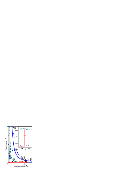
Figure 2: (Color online) Dependence of the transmittance $T$ [see Eq. (22)] on the normalized amplitude $h_{0}$ of the incident magnetic field [see Eq. (21)] for different values of the negative frequency detuning: $(\Omega-1)=-5\cdot 10^{-5}$ (solid curve), $-5\cdot 10^{-4}$ (dashed curve), $-5\cdot 10^{-3}$ (dotted curve). Arrows show the change of the transmittance when changing $h_{0}$. The numbers near the points on the solid $T(h_{0})$ curve correspond to the same numbers of the phase trajectories $a^{\prime}(a)$ shown in Fig. 3. The inset shows the enlarged region near the point 1. The values of the parameters are: $\delta=2$, $\lambda_{c}=4\cdot 10^{-3}$ cm, $\lambda_{ab}=2000$ Å, $\omega_{J}/2\pi=0.3$ THz, and $\theta=45^{\circ}$.

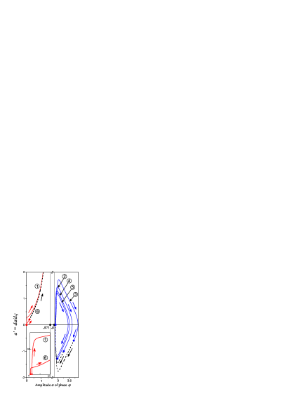
Figure 3: (Color online) Phase trajectories $a^{\prime}(a)$ for the negative frequency detuning $\Omega-1=-5\cdot 10^{-5}$. The numbers near the curves correspond to the same numbers of points in the $T(h_{0})$ plot shown by the solid curve in Fig. 2. The movement along the phase trajectories in the directions shown by the arrows corresponds to the growth of the spatial coordinate $\zeta$ (proportional to $z$), from zero to $\delta$, inside the slab. The solid lines show the portions of the phase trajectories that correspond to $0<\zeta<\delta$. The lower and upper surfaces of the slab correspond to the solid circles on the trajectories. The inset in the bottom left shows the enlarged region near the point $(a=0,\,a^{\prime}=0)$. The other parameters are the same as for Fig. 2.

The low-amplitude (quasi-linear) branch of the $T(h_{0})$ dependence ranges within the interval $0<h_{0}<(8/27)^{1/2}$ of the amplitudes of the incident waves. This branch is shown in Fig. 2 by the red solid curve close to the abscissa. For small amplitudes $h_{0}\ll 1$, we deal with a linear problem, when the phase difference $\varphi$ and the electromagnetic field in the superconductor can be found in the form of linear combinations of exponential functions of $z$. In this case, the transmittance $T$ can be found asymptotically for small $\Gamma$,

$$T(h_{0}\ll 1)\approx\frac{4\Gamma^{4}}{\sinh^{2}\left[\delta(1-\kappa^{-2})\right]+4\Gamma^{4}},\quad\Gamma\ll 1.$$ (23)

This transmittance is very close to zero regardless of the frequency detuning $(\Omega-1)$. As we will see below, the “sinh” above, for $\omega<\omega_{J}$, will become “sin” for $\omega>\omega_{J}$.

The phase trajectories that correspond to the low-amplitude solutions occupy the region $a<(8/3)^{1/2}$. For small $h_{0}$, these trajectories are close to the point $(a=0,\,a^{\prime}=0)$ (as an example of such trajectory, see curve 6 in Fig. 3). An increase of the amplitude $h_{0}$ leads to the growth of the length of the phase trajectory and this length tends to infinity when $h_{0}\rightarrow(8/27)^{1/2}$ (see curve 1 in Fig. 3).

The high-amplitude branches of the $T(h_{0})$ dependence correspond to the solutions with $a(\zeta)>{8}^{1/2}$. Such branches are shown in Fig. 2 by dotted, dashed, and blue solid curves for different values of the frequency detuning. The high-amplitude solutions describe nonlinear Josephson plasma waves that can propagate in the layered superconductor even for negative frequency detuning (for $\Omega<1$). The corresponding phase trajectories are closed curves (see the closed curves in Fig. 3 for $a>{8}^{1/2}$). Note that the value of $h$ is negative for $a>8^{1/2}$. For this case, we can consider $h$ to be positive, but the phase of the incident wave must be shifted by $\pi$.

The oscillating character of the high-amplitude solutions results in much higher values of the transmittance, compared to the case of exponentially-small quasi-linear solutions. As seen in Fig. 2, the transmittance varies over a wide range, from nearly zero to one, depending on the amplitude $h_{0}$ of the incident magnetic field. It is important to note that the wavelengths of the nonlinear waves in the superconductor depend strongly on the incident wave amplitude $h_{0}$. So, changing $h_{0}$ one can control the relation between the wavelength and the thickness of the slab. The transmittance is very sensitive to this relation, and one can attain total transparency of the slab choosing the optimal value $h_{0}^{\rm max}$ of the amplitude $h_{0}$.

For high enough amplitudes $h_{0}$, the sample thickness $D$ is larger than the half-wavelength. In this case, the change of the coordinate $\zeta$ in the interval $0<\zeta<\delta$ corresponds to the movement along a section of the phase trajectory loop (see the trajectories 2, 3, 4 in Fig. 3). When decreasing $h_{0}$, the wavelength increases, the movement along the phase trajectory approaches the complete loop, and the transmittance of the slab increases. Finally, for a specific value of $h_{0}$, the wavelength becomes equal to the sample thickness, the phase trajectory draws a complete loop, and the transmittance becomes equal to one (see the trajectory 5 in Fig. 3 and point 1 in Fig. 2).

The amplitude dependence of the transmittance can be found asymptotically for small values of the parameter $\Gamma$ and for not very thick slabs, $\delta\lesssim 1$,

$$T(h_{0})\,\simeq\,\frac{4\Gamma^{2}}{\delta^{2}}\Big{(}\frac{\delta^{2}}{\sqrt{2}h_{0}}+1\Big{)}^{2}.$$ (24)

In the case of total transparency ($T=1$) of the slab, for $h_{0}^{\rm max}\simeq 2^{1/2}\Gamma\delta$, both the electric and magnetic fields take on the same values on the upper and lower surfaces of the slab. Thus, the amplitudes of the incident and transmitted waves are equal. The corresponding spatial distribution of the magnetic field is shown by the solid curve in Fig. 4.

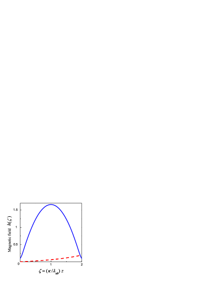
Figure 4: (Color online) Spatial distribution of the amplitude $h$ of the magnetic field inside the superconducting plate. Solid and dashed curves are plotted for the points 5 and 1 shown in Fig. 2, respectively. Point 1 corresponds to the low-amplitude branch of the $T(h_{0})$ dependence, when the transmission coefficient is close to zero, and the amplitude $h$ of the magnetic field near the lower interface ($z=0$) of the slab is exponentially small. The transmittance $T$ for the point 5 is equal to one, and the amplitudes of the fields near the upper and lower interfaces of the slab coincide. Here, the frequency detuning is $(\Omega-1)=-5\cdot 10^{-5}$, and the other parameters are the same as for Fig. 2.

The nontrivial feature of the $T(h_{0})$ dependence can be seen from its hysteretic behavior with jumps. Let the amplitude $h_{0}$ of the incident wave increase from zero. In this case, the transmittance is close to zero, and the $T(h_{0})$ dependence follows the low-amplitude branch shown by the red solid line near the abscissa in Fig. 2. When the amplitude reaches the critical value $(8/27)^{1/2}$ (point 1), further movement along this branch is impossible, and a jump to point 2, on the high-amplitude branch, occurs. A further increase in the amplitude $h_{0}$ results in a monotonic decrease of the transmittance.

Afterwards, if the amplitude $h_{0}$ starts to decrease, then the $T(h_{0})$ dependence does not follow the same track. Indeed, when the point 2 is passed, the transmittance continues to follow the high-amplitude branch. Decreasing the amplitude $h_{0}$ results in a further increase of the transmittance. When it becomes equal to one (point 5), it is not possible to continue the movement along the high-amplitude branch, and a return jump to the low-amplitude branch occurs.

It should be noted that the jump from the low-amplitude branch (which corresponds to the exponentially small transmittance) to the high-amplitude one (with much higher transmittance) can be observed when changing the wave frequency $\omega$ for the constant amplitude $H_{0}$ of the incident wave. This jump occurs when the frequency detuning $(1-\Omega)$ becomes equal to the threshold value

$$\left(1-\Omega_{\rm cr}\right)=\dfrac{3}{4}\left(\lambda_{c}k_{x}\dfrac{H_{0}}{\mathcal{H}_{0}}\right)^{2/3}.$$

III.3 Mechanical analogy

The problem discussed in this paper has a deep and very interesting mechanical analogy. Indeed, Eqs. (16) and Eq. (14) describe a motion of a particle with unite mass in a centrally symmetric potential. The amplitude $h(\zeta)$ of the magnetic field, the phase $\eta(\zeta)$, and the coordinate $\zeta$ across the layers of the superconductor play the roles of the radial coordinate of the particle, its polar angle, and time, respectively. Moreover, the constant $L$ in Eqs. (16) and Eq. (14) can be regarded as the conserved angular momentum of the particle.

Integrating Eq. (16) for the radial motion of the particle, we obtain the energy conservation law for the particle,

$$\dfrac{(h^{\prime})^{2}}{2}+U_{\rm eff}(h)={\cal E},$$ (25)

with the effective potential

$$U_{\rm eff}(h)=\dfrac{L^{2}}{2h^{2}}+\dfrac{h^{2}}{2\kappa}-\int^{h}a(\tilde{h})\,{\rm d}\tilde{h}.$$ (26)

The first term in Eq. (25) describes the kinetic energy of the radial motion of the particle, ${\cal E}$ is the total energy of the particle. The first term in Eq. (26) is the centrifugal energy and the last two terms represent the potential of the central field.

The plot of the dependence $U_{\rm eff}(h)$ is shown in Fig. 5 for the case of negative detuning ($\Omega<1$). This dependence is three-valued and corresponds to the three branches of the function $a(h)$ (see Eq. (15)). Thus, the multivaluedness of the dependence $a(h)$ results in the multivaluedness of the effective potential $U_{\rm eff}(h)$ and, therefore, there exist several possibilities for the particle motion. In terms of our electrodynamical problem, this means that several field distributions in the superconductor can be realized for the same amplitude $h_{0}$ of the incident wave.

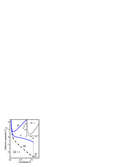
Figure 5: (Color online) Dependence of the effective potential $U_{\rm eff}$ defined by Eq. (26) on the radial coordinate $h$. The movement of the particle in this potential represents the mechanical analog for the spatial distribution of the amplitude $h$ of the magnetic field in the superconductor. The main panel shows curves I, II, and III that correspond to the three branches of the $a(h)$ dependence for the case of negative frequency detuning, $\Omega<1$. The inset shows the $U_{\rm eff}(h)$ curve for the opposite case, $\Omega>1$, when only one branch of the $a(h)$ dependence exists. The value of constant $L$ is $0.1$.

Curve I in Fig. 5 shows the potential that corresponds to the low-amplitude solutions of our electrodynamical problem. The motion of the particle (from right to left) in this potential is monotonic that corresponds to the monotonic decrease of the field deep into the superconductor. According to Eq. (20), the stop-point of the particle ($h^{\prime}=0$) corresponds to the lower boundary of the superconductor.

Since curve I is terminated in the point $h=(32/27)^{1/2}$, it cannot define the particle motion for high enough $h$. In this case, the particle moves in the potential described by curve II in Fig. 5. This motion is finite and periodical. It corresponds to the high-amplitude solutions of our electrodynamical problem. Curve III in Fig. 5 represents a branch of the $U_{\rm eff}(h)$ dependence which cannot be realized when changing the amplitude $h_{0}$ of the incident wave.

III.4 Transmittance of a superconducting slab for $\omega>\omega_{J}$

Now we study the transmittance of a slab of layered superconductors for waves with frequencies higher than the Josephson-plasma frequency, $\Omega>1$. Contrary to the case $\Omega<1$, even linear Josephson plasma waves can propagate in the layered superconductor. Therefore, the transmittance is not exponentially small and can vary over a wide range, depending on the relation between the wavelength and the thickness of the slab:

$$T(h_{0}\ll 1)\approx\frac{4\Gamma^{4}}{\sin^{2}\left[\delta(1-\kappa^{-2})\right]+4\Gamma^{4}},\qquad\Gamma\ll 1.$$ (27)

Note that the “sinh” in Eq. (23), for $\omega<\omega_{J}$, has now been replaced by a “sin” in Eq. (27), for $\omega>\omega_{J}$.

In the nonlinear case, changing the amplitude $h_{0}$, one can control the relation between the wavelength and the thickness of the slab and, thus, the transmittance is tunable by the amplitude of the incident wave. Figure 6 shows the $T(h_{0})$ dependences for different positive frequency detunings.

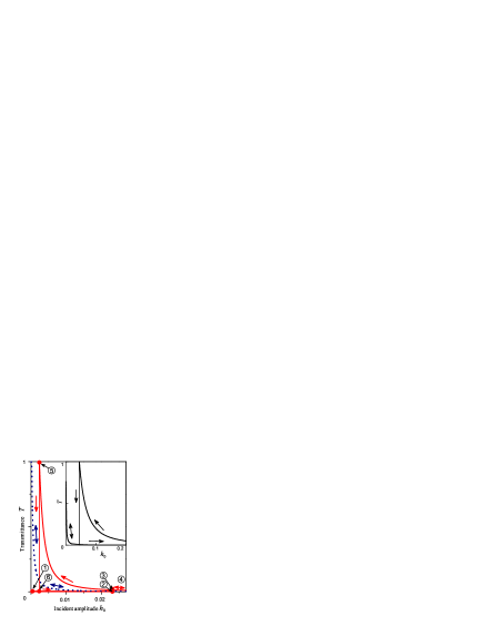
Figure 6: (Color online) Dependence of the transmittance $T$ on the normalized amplitude $h_{0}$ of the incident wave for different positive values of the frequency detuning: $\Omega-1=5\cdot 10^{-3}$, or $\delta/\pi=1.2$ (dotted curve); $\Omega-1=4.5\cdot 10^{-3}$, or $\delta/\pi=1.25$ (solid curve); $\Omega-1=1.65\cdot 10^{-3}$, or $\delta/\pi=2.1$ (inset). Arrows show the change of the transmittance when changing $h_{0}$. The sample thickness is $D=4.3\cdot 10^{-5}$ cm, and other parameters are the same as in Fig. 2.

The analysis based on Eqs. (15) (with choice of the sign “$-$”), (16), (18), (19), (20), and (22) shows that the dependence $T(h_{0})$ is reversible when the frequency detuning is larger than some threshold value, which is defined by the asymptotic equation

$$(\Omega_{\rm thr}-1)\,\approx\,\left(\frac{D\sqrt{\epsilon}\sin\theta}{\sqrt{2}\pi\lambda_{ab}}\right)^{2},\quad\Gamma\ll 1.$$ (28)

An example of such a reversible $T(h_{0})$ dependence is presented by the dotted curve in Fig. 6.

The hysteresis in the $T(h_{0})$ dependence appears for frequency detunings smaller than the threshold value:

$$\Omega<\Omega_{\rm thr}.$$ (29)

In this case, the transmittance can reach the value one when the incident wave amplitude $h_{0}$ is first increased and then decreased. Namely, the incident wave amplitude $h_{0}$ is decreased after it increases and a jump of $T(h_{0})$ occurs from the low-amplitude branch to the high-amplitude one (see the solid curve and the inset in Fig. 6). One can derive the asymptotic equation for the optimal value $h_{0}^{\rm max}$ of $h_{0}$ when the superconducting slab becomes totally transparent,

$$h_{0}^{\rm max}\simeq\frac{3\sqrt{3}}{4I^{2}}\Gamma\delta^{2}$$ (30)

where

$$I=\int\limits_{0}^{1}\frac{dx}{\sqrt{1-x^{4/3}}}\,=\,\frac{3}{4}\,\rm B\Big{(}\frac{1}{2},\frac{3}{4}\Big{)}\,\approx\,1.7972$$

and ${\rm B}(x,y)$ is the Euler integral of the first kind.

III.5 Mechanical analogy revisited

Returning to the mechanical analogy described in the previous subsection, we note that, in the case of positive-frequency detuning, the dependence of the potential $U_{\rm eff}$ on the radial coordinate $h$ of the particle is single-valued (see the inset in Fig. 5). This is because the dependence $a(h)$ in Eq. (15) is single-valued in this case. Nevertheless, the dependence $T(h_{0})$ can be multivalued even for $\Omega>1$ (see Fig. 6). This feature seems to be paradoxical. Indeed, the particle motion is completely defined for any initial conditions. However, an assignment of the value of $h_{0}$ in relations (18), (19), and (20) does not mean an imposition of definite initial conditions for the particle motion. To illustrate this nontrivial feature of the electromagnetic wave transmission through a slab of layered superconductor, let us now consider the inverse problem. We wish to find the amplitude $h_{0}$ of the incident wave that is necessary to obtain a given value $h_{T}$ of the transmitted wave. According to Eq. (19), the value of $h_{T}$ defines unambiguously the angular momentum $L=h_{T}^{2}/\Gamma$ of the particle. On the basis of the motion equation (16) and the boundary condition Eq. (18), we find that the dependence $h_{0}(h_{T})$ should be single-valued. Correspondingly, the dependence of the transmittance

$$T=h_{T}^{2}/h_{0}^{2}$$

on the amplitude $h_{T}$ of the transmitted wave is also single-valued (see Fig. 7). However, this dependence is nonmonotonic if the condition Eq. (29) is satisfied. As a result, the dependence $T(h_{0})$ appears to be multiple-valued.

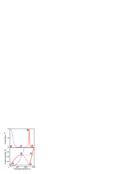
Figure 7: (Color online) Solution of the inverse problem: dependences of the amplitude $h_{0}$ of the incident wave and transmittance $T=h_{T}^{2}/h_{0}^{2}$ on the amplitude $h_{T}$ of the transmitted wave. The values of the parameters and the numbers near the indicated points are the same as in the main panel in Fig. 6. The dependences plotted by dotted curves are monotonic, leading to the single-valued dependence $T(h_{0})$ (the dotted curve in Fig. 6). The solid-and-dashed curves show the nonmonotonic behavior that results in the multivalued dependence $T(h_{0})$ (the solid curve in the main panel in Fig. 6).

IV Conclusion

In this paper we predict a new nonlinear phenomenon in layered superconductors. We show that the reflectivity and transmittance of a superconducting slab are very sensitive to the amplitude of the incident wave due to the nonlinearity of the Josephson relation for the c-axis current. As a result, the reflectivity and transmittance vary over a wide range, from nearly zero to one (if neglecting the small dissipation), when changing the amplitude of the incident electromagnetic wave. A remarkable feature of this phenomenon is the hysteretic behavior of the $T(h_{0})$ dependence. It is important to note that, for frequencies close to the Josephson plasma frequency, the tunable transmittance can vary from zero to one even in the case of weak nonlinearity, when the interlayer phase difference $\varphi$ is small, $\varphi\ll 1$.

V Acknowledgements

We gratefully acknowledge partial support from the Laboratory of Physical Sciences, National Security Agency, Army Research Office, National Science Foundation grant No. 0726909, DARPA, JSPS-RFBR contract No. 09-02-92114, Grant-in-Aid for Scientific Research (S), MEXT Kakenhi on Quantum Cybernetics, Funding Program for Innovative R&D on S&T (FIRST), and Ukrainian State Program on Nanotechnology and Nanomaterials.

References

- (1) S. Savel’ev, V.A. Yampol’skii, A.L. Rakhmanov, and F. Nori, Rep. Prog. Phys. 73, 026501 (2010).
- (2) R. Kleiner, F. Steinmeyer, G. Kunkel, and P. Muller, Phys. Rev. Lett. 68, 2394 (1992).
- (3) R. Kleiner and P. Muller, Phys. Rev. B49, 1327 (1994).
- (4) E.H. Brandt, Rep. Prog. Phys. 58, 1465 (1995).
- (5) V.L. Pokrovsky, Phys. Rep. 288, 325 (1997).
- (6) S. Sakai, P. Bodin, and N.F. Pedersen, J. Appl. Phys 73, 2411 (1993).
- (7) S.N. Artemenko and S.V. Remizov, JETP Lett. 66, 811 (1997).
- (8) S.N. Artemenko and S.V. Remizov, Physica C 362, 200 (2001).
- (9) Ch. Helm, J. Keller, Ch. Peris, and A. Sergeev, Physica C 362, 43 (2001).
- (10) Yu.H. Kim and J. Pokharel, Physica C 384, 425 (2003).
- (11) S. Savel’ev, A.L. Rakhmanov, V.A. Yampol’skii, and F. Nori, Nat. Phys. 2, 521 (2006).
- (12) S. Savel’ev, V.A. Yampol’skii, A.L. Rakhmanov, and F. Nori, Phys. Rev. B 75, 184503 (2007).
- (13) V.A. Yampol’skii, S. Savel’ev, A.L. Rakhmanov, and F. Nori, Phys. Rev. B 78, 024511 (2008).
- (14) V.A. Yampol’skii, S. Savel’ev, T.M. Slipchenko, A.L. Rakhmanov, and F. Nori, Physica C 468, 499 (2008).
- (15) V.A. Yampol’skii, T.M. Slipchenko, Z.A. Mayzelis, D.V. Kadygrob, S.S. Apostolov, S.E. Savel’ev, and F. Nori, Phys. Rev. B 78, 184504 (2008).
- (16) H. Ian, Y.X. Liu, and F. Nori, Phys. Rev. A81, 063823 (2010).
- (17) L. He, Y.X. Liu, S. Yi, C.P. Sun, and F. Nori, Phys. Rev. A75, 063823 (2007).
- (18) Ch. Helm and L.N. Bulaevskii, Phys. Rev. B66, 094514 (2002).