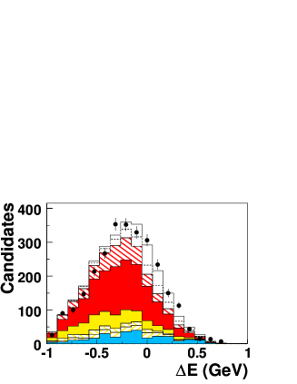
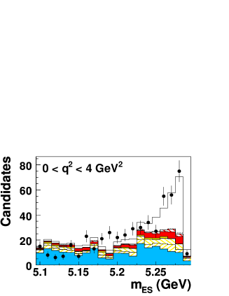
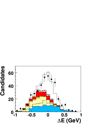
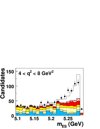
BABAR-PUB-09/037

SLAC-PUB-14106

The BABAR Collaboration

Study of Bπνbold-→𝐵𝜋bold-ℓ𝜈B\rightarrow\pi\ell\nu and Bρνbold-→𝐵𝜌bold-ℓ𝜈B\rightarrow\rho\ell\nu Decays and Determination of |Vub|subscript𝑉𝑢𝑏|V_{ub}|

P. del Amo Sanchez    J. P. Lees    V. Poireau    E. Prencipe    V. Tisserand Laboratoire d’Annecy-le-Vieux de Physique des Particules (LAPP), Université de Savoie, CNRS/IN2P3, F-74941 Annecy-Le-Vieux, France    J. Garra Tico    E. Grauges Universitat de Barcelona, Facultat de Fisica, Departament ECM, E-08028 Barcelona, Spain    M. Martinelliab    A. Palanoab    M. Pappagalloab INFN Sezione di Baria; Dipartimento di Fisica, Università di Barib, I-70126 Bari, Italy    G. Eigen    B. Stugu    L. Sun University of Bergen, Institute of Physics, N-5007 Bergen, Norway    M. Battaglia    D. N. Brown    B. Hooberman    L. T. Kerth    Yu. G. Kolomensky    G. Lynch    I. L. Osipenkov    T. Tanabe Lawrence Berkeley National Laboratory and University of California, Berkeley, California 94720, USA    C. M. Hawkes    N. Soni    A. T. Watson University of Birmingham, Birmingham, B15 2TT, United Kingdom    H. Koch    T. Schroeder Ruhr Universität Bochum, Institut für Experimentalphysik 1, D-44780 Bochum, Germany    D. J. Asgeirsson    C. Hearty    T. S. Mattison    J. A. McKenna University of British Columbia, Vancouver, British Columbia, Canada V6T 1Z1    A. Khan    A. Randle-Conde Brunel University, Uxbridge, Middlesex UB8 3PH, United Kingdom    V. E. Blinov    A. R. Buzykaev    V. P. Druzhinin    V. B. Golubev    A. P. Onuchin    S. I. Serednyakov    Yu. I. Skovpen    E. P. Solodov    K. Yu. Todyshev    A. N. Yushkov Budker Institute of Nuclear Physics, Novosibirsk 630090, Russia    M. Bondioli    S. Curry    D. Kirkby    A. J. Lankford    M. Mandelkern    E. C. Martin    D. P. Stoker University of California at Irvine, Irvine, California 92697, USA    H. Atmacan    J. W. Gary    F. Liu    O. Long    G. M. Vitug    Z. Yasin University of California at Riverside, Riverside, California 92521, USA    V. Sharma University of California at San Diego, La Jolla, California 92093, USA    C. Campagnari    T. M. Hong    D. Kovalskyi    J. D. Richman University of California at Santa Barbara, Santa Barbara, California 93106, USA    A. M. Eisner    C. A. Heusch    J. Kroseberg    W. S. Lockman    A. J. Martinez    T. Schalk    B. A. Schumm    A. Seiden    L. O. Winstrom University of California at Santa Cruz, Institute for Particle Physics, Santa Cruz, California 95064, USA    C. H. Cheng    D. A. Doll    B. Echenard    D. G. Hitlin    P. Ongmongkolkul    F. C. Porter    A. Y. Rakitin California Institute of Technology, Pasadena, California 91125, USA    R. Andreassen    M. S. Dubrovin    G. Mancinelli    B. T. Meadows    M. D. Sokoloff University of Cincinnati, Cincinnati, Ohio 45221, USA    P. C. Bloom    W. T. Ford    A. Gaz    J. F. Hirschauer    M. Nagel    U. Nauenberg    J. G. Smith    S. R. Wagner University of Colorado, Boulder, Colorado 80309, USA    R. Ayad Now at Temple University, Philadelphia, Pennsylvania 19122, USA    W. H. Toki Colorado State University, Fort Collins, Colorado 80523, USA    A. Hauke    H. Jasper    T. M. Karbach    J. Merkel    A. Petzold    B. Spaan    K. Wacker Technische Universität Dortmund, Fakultät Physik, D-44221 Dortmund, Germany    M. J. Kobel    K. R. Schubert    R. Schwierz Technische Universität Dresden, Institut für Kern- und Teilchenphysik, D-01062 Dresden, Germany    D. Bernard    M. Verderi Laboratoire Leprince-Ringuet, CNRS/IN2P3, Ecole Polytechnique, F-91128 Palaiseau, France    P. J. Clark    S. Playfer    J. E. Watson University of Edinburgh, Edinburgh EH9 3JZ, United Kingdom    M. Andreottiab    D. Bettonia    C. Bozzia    R. Calabreseab    A. Cecchiab    G. Cibinettoab    E. Fioravantiab    P. Franchiniab    E. Luppiab    M. Muneratoab    M. Negriniab    A. Petrellaab    L. Piemontesea INFN Sezione di Ferraraa; Dipartimento di Fisica, Università di Ferrarab, I-44100 Ferrara, Italy    R. Baldini-Ferroli    A. Calcaterra    R. de Sangro    G. Finocchiaro    M. Nicolaci    S. Pacetti    P. Patteri    I. M. Peruzzi Also with Università di Perugia, Dipartimento di Fisica, Perugia, Italy    M. Piccolo    M. Rama    A. Zallo INFN Laboratori Nazionali di Frascati, I-00044 Frascati, Italy    R. Contriab    E. Guidoab    M. Lo Vetereab    M. R. Mongeab    S. Passaggioa    C. Patrignaniab    E. Robuttia    S. Tosiab INFN Sezione di Genovaa; Dipartimento di Fisica, Università di Genovab, I-16146 Genova, Italy    B. Bhuyan Indian Institute of Technology Guwahati, Guwahati, Assam, 781 039, India    M. Morii Harvard University, Cambridge, Massachusetts 02138, USA    A. Adametz    J. Marks    S. Schenk    U. Uwer Universität Heidelberg, Physikalisches Institut, Philosophenweg 12, D-69120 Heidelberg, Germany    F. U. Bernlochner    H. M. Lacker    T. Lueck    A. Volk Humboldt-Universität zu Berlin, Institut für Physik, Newtonstr. 15, D-12489 Berlin, Germany    P. D. Dauncey    M. Tibbetts Imperial College London, London, SW7 2AZ, United Kingdom    P. K. Behera    U. Mallik University of Iowa, Iowa City, Iowa 52242, USA    C. Chen    J. Cochran    H. B. Crawley    L. Dong    W. T. Meyer    S. Prell    E. I. Rosenberg    A. E. Rubin Iowa State University, Ames, Iowa 50011-3160, USA    Y. Y. Gao    A. V. Gritsan    Z. J. Guo Johns Hopkins University, Baltimore, Maryland 21218, USA    N. Arnaud    M. Davier    D. Derkach    J. Firmino da Costa    G. Grosdidier    F. Le Diberder    A. M. Lutz    B. Malaescu    A. Perez    P. Roudeau    M. H. Schune    J. Serrano    V. Sordini Also with Università di Roma La Sapienza, I-00185 Roma, Italy    A. Stocchi    L. Wang    G. Wormser Laboratoire de l’Accélérateur Linéaire, IN2P3/CNRS et Université Paris-Sud 11, Centre Scientifique d’Orsay, B. P. 34, F-91898 Orsay Cedex, France    D. J. Lange    D. M. Wright Lawrence Livermore National Laboratory, Livermore, California 94550, USA    I. Bingham    J. P. Burke    C. A. Chavez    J. P. Coleman    J. R. Fry    E. Gabathuler    R. Gamet    D. E. Hutchcroft    D. J. Payne    C. Touramanis University of Liverpool, Liverpool L69 7ZE, United Kingdom    A. J. Bevan    F. Di Lodovico    R. Sacco    M. Sigamani Queen Mary, University of London, London, E1 4NS, United Kingdom    G. Cowan    S. Paramesvaran    A. C. Wren University of London, Royal Holloway and Bedford New College, Egham, Surrey TW20 0EX, United Kingdom    D. N. Brown    C. L. Davis University of Louisville, Louisville, Kentucky 40292, USA    A. G. Denig    M. Fritsch    W. Gradl    A. Hafner Johannes Gutenberg-Universität Mainz, Institut für Kernphysik, D-55099 Mainz, Germany    K. E. Alwyn    D. Bailey    R. J. Barlow    G. Jackson    G. D. Lafferty    T. J. West University of Manchester, Manchester M13 9PL, United Kingdom    J. Anderson    R. Cenci    A. Jawahery    D. A. Roberts    G. Simi    J. M. Tuggle University of Maryland, College Park, Maryland 20742, USA    C. Dallapiccola    E. Salvati University of Massachusetts, Amherst, Massachusetts 01003, USA    R. Cowan    D. Dujmic    P. H. Fisher    G. Sciolla    R. K. Yamamoto    M. Zhao Massachusetts Institute of Technology, Laboratory for Nuclear Science, Cambridge, Massachusetts 02139, USA    P. M. Patel    S. H. Robertson    M. Schram McGill University, Montréal, Québec, Canada H3A 2T8    P. Biassoniab    A. Lazzaroab    V. Lombardoa    F. Palomboab    S. Strackaab INFN Sezione di Milanoa; Dipartimento di Fisica, Università di Milanob, I-20133 Milano, Italy    L. Cremaldi    R. Godang Now at University of South Alabama, Mobile, Alabama 36688, USA    R. Kroeger    P. Sonnek    D. J. Summers    H. W. Zhao University of Mississippi, University, Mississippi 38677, USA    X. Nguyen    M. Simard    P. Taras Université de Montréal, Physique des Particules, Montréal, Québec, Canada H3C 3J7    G. De Nardoab    D. Monorchioab    G. Onoratoab    C. Sciaccaab INFN Sezione di Napolia; Dipartimento di Scienze Fisiche, Università di Napoli Federico IIb, I-80126 Napoli, Italy    G. Raven    H. L. Snoek NIKHEF, National Institute for Nuclear Physics and High Energy Physics, NL-1009 DB Amsterdam, The Netherlands    C. P. Jessop    K. J. Knoepfel    J. M. LoSecco    W. F. Wang University of Notre Dame, Notre Dame, Indiana 46556, USA    L. A. Corwin    K. Honscheid    R. Kass    J. P. Morris    A. M. Rahimi Ohio State University, Columbus, Ohio 43210, USA    N. L. Blount    J. Brau    R. Frey    O. Igonkina    J. A. Kolb    R. Rahmat    N. B. Sinev    D. Strom    J. Strube    E. Torrence University of Oregon, Eugene, Oregon 97403, USA    G. Castelliab    E. Feltresiab    N. Gagliardiab    M. Margoniab    M. Morandina    M. Posoccoa    M. Rotondoa    F. Simonettoab    R. Stroiliab INFN Sezione di Padovaa; Dipartimento di Fisica, Università di Padovab, I-35131 Padova, Italy    E. Ben-Haim    G. R. Bonneaud    H. Briand    J. Chauveau    O. Hamon    Ph. Leruste    G. Marchiori    J. Ocariz    J. Prendki    S. Sitt Laboratoire de Physique Nucléaire et de Hautes Energies, IN2P3/CNRS, Université Pierre et Marie Curie-Paris6, Université Denis Diderot-Paris7, F-75252 Paris, France    M. Biasiniab    E. Manoniab INFN Sezione di Perugiaa; Dipartimento di Fisica, Università di Perugiab, I-06100 Perugia, Italy    C. Angeliniab    G. Batignaniab    S. Bettariniab    G. Calderiniab Also with Laboratoire de Physique Nucléaire et de Hautes Energies, IN2P3/CNRS, Université Pierre et Marie Curie-Paris6, Université Denis Diderot-Paris7, F-75252 Paris, France    M. Carpinelliab Also with Università di Sassari, Sassari, Italy    A. Cervelliab    F. Fortiab    M. A. Giorgiab    A. Lusianiac    N. Neriab    E. Paoloniab    G. Rizzoab    J. J. Walsha INFN Sezione di Pisaa; Dipartimento di Fisica, Università di Pisab; Scuola Normale Superiore di Pisac, I-56127 Pisa, Italy    D. Lopes Pegna    C. Lu    J. Olsen    A. J. S. Smith    A. V. Telnov Princeton University, Princeton, New Jersey 08544, USA    F. Anullia    E. Baracchiniab    G. Cavotoa    R. Facciniab    F. Ferrarottoa    F. Ferroniab    M. Gasperoab    L. Li Gioia    M. A. Mazzonia    G. Pireddaa    F. Rengaab INFN Sezione di Romaa; Dipartimento di Fisica, Università di Roma La Sapienzab, I-00185 Roma, Italy    M. Ebert    T. Hartmann    T. Leddig    H. Schröder    R. Waldi Universität Rostock, D-18051 Rostock, Germany    T. Adye    B. Franek    E. O. Olaiya    F. F. Wilson Rutherford Appleton Laboratory, Chilton, Didcot, Oxon, OX11 0QX, United Kingdom    S. Emery    G. Hamel de Monchenault    G. Vasseur    Ch. Yèche    M. Zito CEA, Irfu, SPP, Centre de Saclay, F-91191 Gif-sur-Yvette, France    M. T. Allen    D. Aston    D. J. Bard    R. Bartoldus    J. F. Benitez    C. Cartaro    M. R. Convery    J. C. Dingfelder Now at Physikalisches Institut Freiburg, Hermann-Herder-Strasse 3, 79104 Freiburg, Germany    J. Dorfan    G. P. Dubois-Felsmann    W. Dunwoodie    R. C. Field    M. Franco Sevilla    B. G. Fulsom    A. M. Gabareen    M. T. Graham    P. Grenier    C. Hast    W. R. Innes    M. H. Kelsey    H. Kim    P. Kim    M. L. Kocian    D. W. G. S. Leith    S. Li    B. Lindquist    S. Luitz    V. Luth    H. L. Lynch    D. B. MacFarlane    H. Marsiske    D. R. Muller    H. Neal    S. Nelson    C. P. O’Grady    I. Ofte    M. Perl    B. N. Ratcliff    A. Roodman    A. A. Salnikov    R. H. Schindler    J. Schwiening    A. Snyder    D. Su    M. K. Sullivan    K. Suzuki    J. M. Thompson    J. Va’vra    A. P. Wagner    M. Weaver    C. A. West    W. J. Wisniewski    M. Wittgen    D. H. Wright    H. W. Wulsin    A. K. Yarritu    V. Santoro    C. C. Young    V. Ziegler SLAC National Accelerator Laboratory, Stanford, California 94309 USA    X. R. Chen    W. Park    M. V. Purohit    R. M. White    J. R. Wilson University of South Carolina, Columbia, South Carolina 29208, USA    S. J. Sekula Southern Methodist University, Dallas, Texas 75275, USA    M. Bellis    P. R. Burchat    A. J. Edwards    T. S. Miyashita Stanford University, Stanford, California 94305-4060, USA    S. Ahmed    M. S. Alam    J. A. Ernst    B. Pan    M. A. Saeed    S. B. Zain State University of New York, Albany, New York 12222, USA    N. Guttman    A. Soffer Tel Aviv University, School of Physics and Astronomy, Tel Aviv, 69978, Israel    P. Lund    S. M. Spanier University of Tennessee, Knoxville, Tennessee 37996, USA    R. Eckmann    J. L. Ritchie    A. M. Ruland    C. J. Schilling    R. F. Schwitters    B. C. Wray University of Texas at Austin, Austin, Texas 78712, USA    J. M. Izen    X. C. Lou University of Texas at Dallas, Richardson, Texas 75083, USA    F. Bianchiab    D. Gambaab    M. Pelliccioniab INFN Sezione di Torinoa; Dipartimento di Fisica Sperimentale, Università di Torinob, I-10125 Torino, Italy    M. Bombenab    G. Della Riccaab    L. Lanceriab    L. Vitaleab INFN Sezione di Triestea; Dipartimento di Fisica, Università di Triesteb, I-34127 Trieste, Italy    V. Azzolini    N. Lopez-March    F. Martinez-Vidal    D. A. Milanes    A. Oyanguren IFIC, Universitat de Valencia-CSIC, E-46071 Valencia, Spain    J. Albert    Sw. Banerjee    H. H. F. Choi    K. Hamano    G. J. King    R. Kowalewski    M. J. Lewczuk    I. M. Nugent    J. M. Roney    R. J. Sobie University of Victoria, Victoria, British Columbia, Canada V8W 3P6    T. J. Gershon    P. F. Harrison    J. Ilic    T. E. Latham    G. B. Mohanty    E. M. T. Puccio Department of Physics, University of Warwick, Coventry CV4 7AL, United Kingdom    H. R. Band    X. Chen    S. Dasu    K. T. Flood    Y. Pan    R. Prepost    C. O. Vuosalo    S. L. Wu University of Wisconsin, Madison, Wisconsin 53706, USA
Abstract

We present an analysis of exclusive charmless semileptonic B𝐵B-meson decays based on 377 million BB¯𝐵¯𝐵B\overline{B} pairs recorded with the BABAR detector at the Υ(4S)Υ4𝑆\mathchar 28935\relax(4S) resonance. We select four event samples corresponding to the decay modes B0π+νsuperscript𝐵0superscript𝜋superscript𝜈B^{0}\rightarrow\pi^{-}\ell^{+}\nu, B+π0+νsuperscript𝐵superscript𝜋0superscript𝜈B^{+}\rightarrow\pi^{0}\ell^{+}\nu, B0ρ+νsuperscript𝐵0superscript𝜌superscript𝜈B^{0}\rightarrow\rho^{-}\ell^{+}\nu, and B+ρ0+νsuperscript𝐵superscript𝜌0superscript𝜈B^{+}\rightarrow\rho^{0}\ell^{+}\nu, and find the measured branching fractions to be consistent with isospin symmetry. Assuming isospin symmetry, we combine the two Bπν𝐵𝜋𝜈B\rightarrow\pi\ell\nu samples, and similarly the two Bρν𝐵𝜌𝜈B\rightarrow\rho\ell\nu samples, and measure the branching fractions (B0π+ν)=(1.41±0.05±0.07)×104superscript𝐵0superscript𝜋superscript𝜈plus-or-minus1.410.050.07superscript104{\cal B}(B^{0}\rightarrow\pi^{-}\ell^{+}\nu)=(1.41\pm 0.05\pm 0.07)\times 10^{-4} and (B0ρ+ν)=(1.75±0.15±0.27)×104superscript𝐵0superscript𝜌superscript𝜈plus-or-minus1.750.150.27superscript104{\cal B}(B^{0}\rightarrow\rho^{-}\ell^{+}\nu)=(1.75\pm 0.15\pm 0.27)\times 10^{-4}, where the errors are statistical and systematic. We compare the measured distribution in q2superscript𝑞2q^{2}, the momentum transfer squared, with predictions for the form factors from QCD calculations and determine the CKM matrix element |Vub|subscript𝑉𝑢𝑏|V_{ub}|. Based on the measured partial branching fraction for Bπν𝐵𝜋𝜈B\rightarrow\pi\ell\nu in the range q2<12GeV2superscript𝑞212superscriptGeV2q^{2}<12\mathrm{\,Ge\kern-1.00006ptV}^{2} and the most recent LCSR calculations we obtain |Vub|=(3.78±0.130.40+0.55)×103subscript𝑉𝑢𝑏plus-or-minus3.78subscriptsuperscript0.130.550.40superscript103|V_{ub}|=(3.78\pm 0.13^{+0.55}_{-0.40})\times 10^{-3}, where the errors refer to the experimental and theoretical uncertainties. From a simultaneous fit to the data over the full q2superscript𝑞2q^{2} range and the FNAL/MILC lattice QCD results, we obtain |Vub|=(2.95±0.31)×103subscript𝑉𝑢𝑏plus-or-minus2.950.31superscript103|V_{ub}|=(2.95\pm 0.31)\times 10^{-3} from Bπν𝐵𝜋𝜈B\rightarrow\pi\ell\nu, where the error is the combined experimental and theoretical uncertainty.

pacs:
13.20.He, 12.15.Hh, 12.38.Qk, 14.40.Nd
preprint: BABAR-PUB-09/037preprint: SLAC-PUB-14106

I Introduction

The elements of the Cabibbo-Kobayashi-Maskawa (CKM) quark-mixing matrix are fundamental parameters of the Standard Model (SM) of electroweak interactions. With the increasingly precise measurements of decay-time-dependent CP𝐶𝑃C\!P asymmetries in B𝐵B-meson decays, in particular sin(2β𝛽\betabeta ; phi1 , improved measurements of the magnitude of Vubsubscript𝑉𝑢𝑏V_{ub} and Vcbsubscript𝑉𝑐𝑏V_{cb} will allow for more stringent experimental tests of the SM mechanism for CP𝐶𝑃C\!P violation sm . This is best illustrated in terms of the unitarity triangle, the graphical representation of one of the unitarity conditions for the CKM matrix, for which the length of the side that is opposite to the angle β𝛽\beta is proportional to the ratio |Vub|/|Vcb|subscript𝑉𝑢𝑏subscript𝑉𝑐𝑏|V_{ub}|/|V_{cb}|. The best method to determine |Vub|subscript𝑉𝑢𝑏|V_{ub}| and |Vcb|subscript𝑉𝑐𝑏|V_{cb}| is to measure semileptonic decay rates for BXcν𝐵subscript𝑋𝑐𝜈B\rightarrow X_{c}\ell\nu and BXuν𝐵subscript𝑋𝑢𝜈B\rightarrow X_{u}\ell\nu (Xcsubscript𝑋𝑐X_{c} and Xusubscript𝑋𝑢X_{u} refer to hadronic states with or without charm), which are proportional to |Vcb|2superscriptsubscript𝑉𝑐𝑏2|V_{cb}|^{2} and |Vub|2superscriptsubscript𝑉𝑢𝑏2|V_{ub}|^{2}, respectively.

There are two methods to extract these two CKM elements from B𝐵B decays, one based on inclusive and the other on exclusive semileptonic decays. Exclusive decays offer better kinematic constraints and thus more effective background suppression than inclusive decays, but the lower branching fractions result in lower event yields. Since the experimental and theoretical techniques for these two approaches are different and largely independent, they can provide important cross checks of our understanding of the theory and the measurements. An overview of the determination of |Vub|subscript𝑉𝑢𝑏|V_{ub}| using both approaches can be found in a recent review kowalewski_mannel .

In this paper, we present a study of four exclusive charmless semileptonic decay modes, B0π+νsuperscript𝐵0superscript𝜋superscript𝜈B^{0}\rightarrow\pi^{-}\ell^{+}\nu, B+π0+νsuperscript𝐵superscript𝜋0superscript𝜈B^{+}\rightarrow\pi^{0}\ell^{+}\nu, B0ρ+νsuperscript𝐵0superscript𝜌superscript𝜈B^{0}\rightarrow\rho^{-}\ell^{+}\nu, and B+ρ0+νsuperscript𝐵superscript𝜌0superscript𝜈B^{+}\rightarrow\rho^{0}\ell^{+}\nu charge_conjugate , and a determination of |Vub|subscript𝑉𝑢𝑏|V_{ub}|. Here \ell refers to a charged lepton, either e+superscript𝑒e^{+} or μ+superscript𝜇\mu^{+}, and ν𝜈\nu refers to a neutrino, either νesubscript𝜈𝑒\nu_{e} or νμsubscript𝜈𝜇\nu_{\mu}. This analysis represents an update of an earlier measurement pilnu_jochen that was based on a significantly smaller data set. For the current analysis, the signal yields and background suppression have been improved and the systematic uncertainties have been reduced through the use of improved reconstruction and signal extraction methods, combined with more detailed background studies.

The principal experimental challenge is the separation of the BXuν𝐵subscript𝑋𝑢𝜈B\rightarrow X_{u}\ell\nu from the dominant BXcν𝐵subscript𝑋𝑐𝜈B\rightarrow X_{c}\ell\nu decays, for which the inclusive branching fraction is a factor of 50 larger. Furthermore, the isolation of individual exclusive charmless decays from all other BXuν𝐵subscript𝑋𝑢𝜈B\rightarrow X_{u}\ell\nu decays is difficult, because the exclusive branching ratios are typically only 10% of (BXuν)=(2.29±0.34)×103𝐵subscript𝑋𝑢𝜈plus-or-minus2.290.34superscript103{\cal B}(B\rightarrow X_{u}\ell\nu)=(2.29\pm 0.34)\times 10^{-3} PDG2008 , the inclusive branching fraction for charmless semileptonic B𝐵B decays.

The reconstruction of signal decays in e+eΥ(4S)BB¯superscript𝑒superscript𝑒Υ4𝑆𝐵¯𝐵e^{+}e^{-}\rightarrow\mathchar 28935\relax{(4S)}\rightarrow B\kern 1.79993pt\overline{\kern-1.79993ptB}{} events requires the identification of three types of particles, the hadronic state Xusubscript𝑋𝑢X_{u} producing one or two charged and/or neutral final state pions, the charged lepton, and the neutrino. The presence of the neutrino is inferred from the missing momentum and energy in the whole event.

The event yields for each of the four signal decay modes are extracted from a binned maximum-likelihood fit to the three-dimensional distributions of the variables mESsubscript𝑚ESm_{\rm ES}, the energy-substituted B𝐵B-meson mass, ΔEΔ𝐸\Delta E, the difference between the reconstructed and the expected B𝐵B-meson energy, and q2superscript𝑞2q^{2}, the momentum transfer squared from the B𝐵B meson to the final-state hadron. The measured differential decay rates in combination with recent form-factor calculations are used to determine |Vub|subscript𝑉𝑢𝑏|V_{ub}|. By measuring both Bπν𝐵𝜋𝜈B\rightarrow\pi\ell\nu and Bρν𝐵𝜌𝜈B\rightarrow\rho\ell\nu decays simultaneously, we reduce the sensitivity to the cross feed between these two decay modes and some of the background contributions.

The most promising decay mode for a precise determination of |Vub|subscript𝑉𝑢𝑏|V_{ub}|, both experimentally and theoretically, is the Bπν𝐵𝜋𝜈B\rightarrow\pi\ell\nu decay for which a number of measurements exist. The first measurement of this type was performed by the CLEO Collaboration pilnu_cleo . In addition to the earlier BABAR measurement mentioned above pilnu_jochen , there is a more recent BABAR measurement pilnu_cote in which somewhat looser criteria on the neutrino selection were applied, resulting in a larger signal sample but also substantially higher backgrounds. These analyses also rely on the measurement of the missing energy and momentum of the whole event to reconstruct the neutrino, without explicitly reconstructing the second B𝐵B-meson decay in the event, but are based on smaller data sets than the one presented here. Recently a number of measurements of both Bπν𝐵𝜋𝜈B\rightarrow\pi\ell\nu and Bρν𝐵𝜌𝜈B\rightarrow\rho\ell\nu decays were published, in which the BB¯𝐵¯𝐵B\kern 1.79993pt\overline{\kern-1.79993ptB}{} events were tagged by a fully reconstructed hadronic or semileptonic decay of the second B𝐵B meson in the event pilnu_babar_tag ; pilnu_belle_tag . These analyses have led to a simpler and more precise reconstruction of the neutrino and very low backgrounds. However, this is achieved at the expense of much smaller signal samples, which limit the statistical precision of the form-factor measurement.

II Form Factors

II.1 Overview

The advantage of charmless semileptonic decays over charmless hadronic decays of the B𝐵B meson is that the leptonic and hadronic components of the matrix element factorize. The hadronic matrix element is difficult to calculate, since it must take into account physical mesons, rather than free quarks. Therefore higher-order perturbative corrections and non-perturbative long-distance hadronization processes cannot be ignored. To overcome these difficulties, a set of Lorentz-invariant form factors has been introduced that give a global description of these QCD processes.

A variety of theoretical predictions for these form factors exist. They are based on QCD calculations, such as lattice QCD and sum rules, in addition to quark models. We will make use of a variety of these calculations to assess their impact on the determination of |Vub|subscript𝑉𝑢𝑏|V_{ub}| from measurements of the decay rates.

The VA𝑉𝐴V-A structure of the hadronic current is invoked, along with the knowledge of the transformation properties of the final-state meson, to formulate these form factors. They are functions of q2=mW2superscript𝑞2subscriptsuperscript𝑚2𝑊q^{2}=m^{2}_{W}, the mass squared of the virtual W𝑊W,

q2superscript𝑞2\displaystyle q^{2} =\displaystyle= (P+Pν)2superscriptsubscript𝑃subscript𝑃𝜈2\displaystyle(P_{\ell}+P_{\nu})^{2} (1)
=\displaystyle= (PBPX)2=MB2+mX22MBEX.superscriptsubscript𝑃𝐵subscript𝑃𝑋2superscriptsubscript𝑀𝐵2subscriptsuperscript𝑚2𝑋2subscript𝑀𝐵subscript𝐸𝑋\displaystyle(P_{B}-P_{X})^{2}=M_{B}^{2}+m^{2}_{X}-2M_{B}E_{X}.

Here Psubscript𝑃P_{\ell} and Pνsubscript𝑃𝜈P_{\nu} refer to the four-momenta of the charged lepton and the neutrino, MBsubscript𝑀𝐵M_{B} and PBsubscript𝑃𝐵P_{B} to the mass and the four-momentum of the B𝐵B meson, and mXsubscript𝑚𝑋m_{X} and EXsubscript𝐸𝑋E_{X} are the mass and energy (in the B𝐵B-meson rest frame) of the final-state meson Xusubscript𝑋𝑢X_{u}.

We distinguish two main categories of exclusive semileptonic decays: decays to pseudoscalar mesons, Bπν𝐵𝜋𝜈B\rightarrow\pi\ell\nu or B+η+νsuperscript𝐵𝜂superscript𝜈B^{+}\rightarrow\eta\ell^{+}\nu, and decays to vector mesons, Bρν𝐵𝜌𝜈B\rightarrow\rho\ell\nu or B+ω+νsuperscript𝐵𝜔superscript𝜈B^{+}\rightarrow\omega\ell^{+}\nu.

Refer to caption
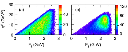
Figure 1: Simulated distributions of q2superscript𝑞2q^{2} versus Esubscript𝐸E_{\ell} for a) Bπν𝐵𝜋𝜈B\rightarrow\pi\ell\nu and b) Bρν𝐵𝜌𝜈B\rightarrow\rho\ell\nu decays. Esubscript𝐸E_{\ell} is the lepton energy in the B𝐵B-meson rest frame.

Figure 1 shows the phase space for Bπν𝐵𝜋𝜈B\rightarrow\pi\ell\nu and Bρν𝐵𝜌𝜈B\rightarrow\rho\ell\nu decays in terms of q2superscript𝑞2q^{2} and Esubscript𝐸E_{\ell}, the energy of the charged lepton in the B𝐵B-meson rest frame. The difference between the distributions is due to the different spin structure of the decays.

II.2 Form Factors

II.2.1 B𝐵B Decays to Pseudoscalar Mesons: Bπν𝐵𝜋𝜈B\rightarrow\pi\ell\nu

For decays to a final-state pseudoscalar meson, the hadronic matrix element is usually written in terms of two form factors, f+(q2)subscript𝑓superscript𝑞2f_{+}(q^{2}) and f0(q2)subscript𝑓0superscript𝑞2f_{0}(q^{2})  neubert94 ; richman-burchat ,

π(Pπ)|u¯γμb|B(PB)=quantum-operator-product𝜋subscript𝑃𝜋¯𝑢superscript𝛾𝜇𝑏𝐵subscript𝑃𝐵absent\displaystyle\langle\pi(P_{\pi})|\overline{u}\gamma^{\mu}b|B(P_{B})\rangle= (2)
f+(q2)[(PB+Pπ)μMB2mπ2q2qμ]+limit-fromsubscript𝑓superscript𝑞2delimited-[]superscriptsubscript𝑃𝐵subscript𝑃𝜋𝜇superscriptsubscript𝑀𝐵2superscriptsubscript𝑚𝜋2superscript𝑞2superscript𝑞𝜇\displaystyle f_{+}(q^{2})\left[(P_{B}+P_{\pi})^{\mu}-\frac{M_{B}^{2}-m_{\pi}^{2}}{q^{2}}\,q^{\mu}\right]+
f0(q2)MB2mπ2q2qμ,subscript𝑓0superscript𝑞2superscriptsubscript𝑀𝐵2superscriptsubscript𝑚𝜋2superscript𝑞2superscript𝑞𝜇\displaystyle\mbox{}f_{0}(q^{2})\,\frac{M_{B}^{2}-m_{\pi}^{2}}{q^{2}}\,q^{\mu},

where Pπsubscript𝑃𝜋P_{\pi} and PBsubscript𝑃𝐵P_{B} are the four-momenta of the final-state pion and the parent B𝐵B meson, and mπsubscript𝑚𝜋m_{\pi} and MBsubscript𝑀𝐵M_{B} are their masses. This expression can be simplified for leptons with small masses, such as electrons and muons, because in the limit of mMBmuch-less-thansubscript𝑚subscript𝑀𝐵m_{\ell}\ll M_{B} the second term can be neglected. We are left with a single form factor f+(q2)subscript𝑓superscript𝑞2f_{+}(q^{2}) and the differential decay rate becomes

dΓ(B0π+ν)dq2dcosθW=|Vub|2GF2pπ332π3sin2θW|f+(q2)|2,𝑑Γsuperscript𝐵0superscript𝜋superscript𝜈𝑑superscript𝑞2𝑑subscript𝜃𝑊superscriptsubscript𝑉𝑢𝑏2subscriptsuperscript𝐺2𝐹superscriptsubscript𝑝𝜋332superscript𝜋3superscript2subscript𝜃𝑊superscriptsubscript𝑓superscript𝑞22\displaystyle\frac{d\Gamma(B^{0}\rightarrow\pi^{-}\ell^{+}\nu)}{dq^{2}d\cos\theta_{W\ell}}=|V_{ub}|^{2}\frac{G^{2}_{F}\,p_{\pi}^{3}}{32\pi^{3}}{\sin}^{2}\theta_{W\ell}|f_{+}(q^{2})|^{2}, (3)

where pπsubscript𝑝𝜋p_{\pi} is the momentum of the pion in the rest frame of the B𝐵B meson, and q2superscript𝑞2q^{2} varies from zero to qmax2=(MBmπ)2subscriptsuperscript𝑞2𝑚𝑎𝑥superscriptsubscript𝑀𝐵subscript𝑚𝜋2q^{2}_{max}=(M_{B}-m_{\pi})^{2}.

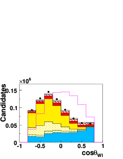
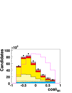
The decay rate depends on the third power of the pion momentum, suppressing the rate at high q2superscript𝑞2q^{2}. The rate also depends on sin2θWsuperscript2subscript𝜃𝑊\sin^{2}\theta_{W\ell}, where θWsubscript𝜃𝑊\theta_{W\ell} is the angle of the charged-lepton momentum in the W𝑊W rest frame with respect to direction of the W𝑊W boost from the B𝐵B rest frame. The combination of these two factors leads to a lepton-momentum spectrum that is peaked well below the kinematic limit (see Figure 1).

II.2.2 B𝐵B Decays to Vector Mesons: Bρν𝐵𝜌𝜈B\rightarrow\rho\ell\nu

For decays with a vector meson in the final state, the polarization vector ϵitalic-ϵ\epsilon of the vector meson plays an important role. The hadronic current is written in terms of four form factors, of which only three (Aisubscript𝐴𝑖A_{i} with i=0,1,2𝑖012i=0,1,2) are independent  neubert94 ; richman-burchat ,

ρ(Pρ,ϵ)|VμAμ|B(PB)=2iV(q2)MB+mρϵμναβϵνPραPBβquantum-operator-product𝜌subscript𝑃𝜌italic-ϵsuperscript𝑉𝜇superscript𝐴𝜇𝐵subscript𝑃𝐵2𝑖𝑉superscript𝑞2subscript𝑀𝐵subscript𝑚𝜌superscriptitalic-ϵ𝜇𝜈𝛼𝛽subscriptsuperscriptitalic-ϵ𝜈subscript𝑃𝜌𝛼subscript𝑃𝐵𝛽\displaystyle\langle\rho(P_{\rho},\epsilon)|V^{\mu}-A^{\mu}|B(P_{B})\rangle=\frac{2iV(q^{2})}{M_{B}+m_{\rho}}\epsilon^{\mu\nu\alpha\beta}\epsilon^{*}_{\nu}P_{\rho\alpha}P_{B\beta} (4)
(MB+mρ)A1(q2)ϵμ+A2(q2)MB+mρϵPB(PB+Pρ)μsubscript𝑀𝐵subscript𝑚𝜌subscript𝐴1superscript𝑞2superscriptitalic-ϵabsent𝜇subscript𝐴2superscript𝑞2subscript𝑀𝐵subscript𝑚𝜌superscriptitalic-ϵsubscript𝑃𝐵superscriptsubscript𝑃𝐵subscript𝑃𝜌𝜇\displaystyle-(M_{B}{+}m_{\rho})A_{1}(q^{2})\epsilon^{*\,\mu}+\frac{A_{2}(q^{2})}{M_{B}{+}m_{\rho}}\epsilon^{*}\!\cdot P_{B}\,(P_{B}{+}P_{\rho})^{\mu}
+2mρϵPBq2qμ[A3(q2)A0(q2)],2subscript𝑚𝜌superscriptitalic-ϵsubscript𝑃𝐵superscript𝑞2superscript𝑞𝜇delimited-[]subscript𝐴3superscript𝑞2subscript𝐴0superscript𝑞2\displaystyle+2m_{\rho}\frac{\epsilon^{*}\!\cdot P_{B}}{q^{2}}q^{\mu}[A_{3}(q^{2})-A_{0}(q^{2})],

where mρsubscript𝑚𝜌m_{\rho} and Pρsubscript𝑃𝜌P_{\rho} refer to the vector-meson mass and four-momentum. Again, a simplification can be made for low-mass charged leptons. The term with qμsuperscript𝑞𝜇q^{\mu} can be neglected, so there are effectively only three form factors for electrons and muons: the axial-vector form factors, A1(q2)subscript𝐴1superscript𝑞2A_{1}(q^{2}) and A2(q2)subscript𝐴2superscript𝑞2A_{2}(q^{2}), and the vector form factor, V(q2)𝑉superscript𝑞2V(q^{2}). Instead of using these form factors, the full differential decay rate is usually expressed in terms of the helicity amplitudes corresponding to the three helicity states of the ρ𝜌\rho meson,

H±(q2)subscript𝐻plus-or-minussuperscript𝑞2\displaystyle H_{\pm}(q^{2}) =\displaystyle= (MB+mρ)[A1(q2)2MBpρ(MB+mρ)2V(q2)],subscript𝑀𝐵subscript𝑚𝜌delimited-[]minus-or-plussubscript𝐴1superscript𝑞22subscript𝑀𝐵subscript𝑝𝜌superscriptsubscript𝑀𝐵subscript𝑚𝜌2𝑉superscript𝑞2\displaystyle(M_{B}+m_{\rho})\bigg{[}A_{1}(q^{2})\mp\frac{2M_{B}\,p_{\rho}}{(M_{B}+m_{\rho})^{2}}V(q^{2})\bigg{]},
H0(q2)subscript𝐻0superscript𝑞2\displaystyle H_{0}(q^{2}) =\displaystyle= MB+mρ2mρq2×[(MB2mρ2q2)A1(q2)\displaystyle\frac{M_{B}+m_{\rho}}{2m_{\rho}\sqrt{q^{2}}}\times\bigg{[}(M_{B}^{2}-m_{\rho}^{2}-q^{2})A_{1}(q^{2}) (5)
\displaystyle- 4MB2pρ2(MB+mρ)2A2(q2)],\displaystyle\frac{4M_{B}^{2}\,p_{\rho}^{2}}{(M_{B}+m_{\rho})^{2}}A_{2}(q^{2})\bigg{]},

where pρsubscript𝑝𝜌p_{\rho} is the momentum of the final-state ρ𝜌\rho meson in the B𝐵B rest frame. While A1subscript𝐴1A_{1} dominates the three helicity amplitudes, A2subscript𝐴2A_{2} contributes only to H0subscript𝐻0H_{0}, and V𝑉V contributes only to H±subscript𝐻plus-or-minusH_{\pm}.

Thus the differential decay rate can be written as

dΓ(Bρν)dq2dcosθW=|Vub|2GF2pρq2128π3MB2×[sinθW2|H0|2\displaystyle\frac{d\Gamma(B\rightarrow\rho\ell\nu)}{dq^{2}d\cos{\theta_{W\ell}}}=|V_{ub}|^{2}\,\frac{G^{2}_{F}\,p_{\rho}\,q^{2}}{128\pi^{3}M_{B}^{2}}\times{}\bigg{[}\sin{\theta^{2}_{W\ell}}|H_{0}|^{2} (6)
+(1cosθW)2|H+|22+(1+cosθW)2|H|22].\displaystyle+(1-\cos{\theta_{W\ell}})^{2}\frac{|H_{+}|^{2}}{2}+(1+\cos{\theta_{W\ell}})^{2}\frac{|H_{-}|^{2}}{2}\bigg{]}.

The VA𝑉𝐴V{-}A nature of the charged weak current leads to a dominant contribution from Hsubscript𝐻H_{-} and a distribution of events characterized by a forward peak in cosθWsubscript𝜃𝑊\cos\theta_{W\ell} and high lepton momenta (see Figure 1).

II.3 Form-Factor Calculations and Models

The q2superscript𝑞2q^{2} dependence of the form factors can be extracted from the data. Since the differential decay rates are proportional to the product of |Vub|2superscriptsubscript𝑉𝑢𝑏2|V_{ub}|^{2} and the form-factor terms, we need at least one point in q2superscript𝑞2q^{2} at which the form factor is predicted in order to extract |Vub|subscript𝑉𝑢𝑏|V_{ub}| from the measured branching fractions.

Currently predictions of form factors are based on

These calculations will also be used to simulate the kinematics of the signal decay modes and thus might impact the detection efficiency and thereby the branching-fraction measurement. The two QCD calculations result in predictions for different regions of phase space. The lattice calculations are only available in the high-q2superscript𝑞2q^{2} region, while LCSR provide information near q2=0superscript𝑞20q^{2}=0. Interpolations between these two regions can be constrained by unitarity and analyticity requirements BGL ; BHill .

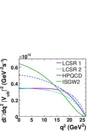
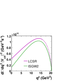
Figure 2 shows the q2superscript𝑞2q^{2} distributions for Bπν𝐵𝜋𝜈B\rightarrow\pi\ell\nu and Bρν𝐵𝜌𝜈B\rightarrow\rho\ell\nu decays for various form-factor calculations. The uncertainties in these predictions are not indicated. For Bπν𝐵𝜋𝜈B\rightarrow\pi\ell\nu decays they are largest at low q2superscript𝑞2q^{2} for LQCD predictions and largest at high q2superscript𝑞2q^{2} for LCSR calculations. Estimates of the uncertainties of the calculations are currently not available for Bρν𝐵𝜌𝜈B\rightarrow\rho\ell\nu decays.

Refer to caption
Refer to caption
Figure 2: q2superscript𝑞2q^{2} distributions for Bπν𝐵𝜋𝜈B\rightarrow\pi\ell\nu (left) and Bρν𝐵𝜌𝜈B\rightarrow\rho\ell\nu (right) decays, based on form-factor predictions from the ISGW2 model isgw2 , LCSR calculations (LCSR 1 ball_pi and LCSR 2 Siegen for Bπν𝐵𝜋𝜈B\rightarrow\pi\ell\nu and LCSR ball_rho for Bρν𝐵𝜌𝜈B\rightarrow\rho\ell\nu) and the HPQCD hpqcd04 lattice calculation. The extrapolations of the QCD predictions to the full q2superscript𝑞2q^{2} range are marked as dashed lines.

The Isgur-Scora-Grinstein-Wise model (ISGW2) isgw2 is a constituent quark model with relativistic corrections. Predictions extend over the full q2superscript𝑞2q^{2} range; they are normalized at q2qmax2superscript𝑞2subscriptsuperscript𝑞2𝑚𝑎𝑥q^{2}\approx q^{2}_{max}. The form factors are parameterized as

f+(q2)=f(qmax2)(1+16Nξ2(qmax2q2))N,subscript𝑓superscript𝑞2𝑓subscriptsuperscript𝑞2𝑚𝑎𝑥superscript116𝑁superscript𝜉2subscriptsuperscript𝑞2𝑚𝑎𝑥superscript𝑞2𝑁f_{+}(q^{2})=f(q^{2}_{max})\left(1+\frac{1}{6N}\xi^{2}(q^{2}_{max}-q^{2})\right)^{-N}\ , (7)

where ξ𝜉\xi is the charge radius of the final-state meson, and N=2𝑁2N=2 (N=3𝑁3N=3) for decays to pseudoscalar (vector) mesons. The uncertainties of the predictions by this model are difficult to quantify.

QCD light-cone sum-rule calculations are non-perturbative and combine the idea of QCD sum rules with twist expansions performed to 𝒪(αs)𝒪subscript𝛼𝑠{\cal O}(\alpha_{s}). These calculations provide estimates of various form factors at low to intermediate q2superscript𝑞2q^{2}, for both pseudoscalar and vector decays. The overall normalization is predicted at low q2superscript𝑞2q^{2} with typical uncertainties of 10-13% ball_pi ; ball_rho .

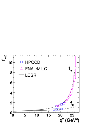
Lattice QCD calculations can potentially provide heavy-to-light-quark form factors from first principles. Unquenched lattice calculations, in which quark-loop effects in the QCD vacuum are incorporated, are now available for the Bπν𝐵𝜋𝜈B\rightarrow\pi\ell\nu form factors from the Fermilab/MILC  fnal09 and the HPQCD hpqcd04 Collaborations. Both calculations account for three dynamical quark flavors, the mass-degenerate u𝑢u and d𝑑d quarks and a heavier s𝑠s quark, but they differ in the way the b𝑏b quark is simulated. Predictions for f0(q2)subscript𝑓0superscript𝑞2f_{0}(q^{2}) and f+(q2)subscript𝑓superscript𝑞2f_{+}(q^{2}) are shown in Figure 3. The two lattice calculations agree within the stated uncertainties, which are significantly smaller than those of earlier quenched approximations.
Refer to caption
Figure 3: (color online) Predictions of the form factors f+subscript𝑓f_{+} and f0subscript𝑓0f_{0} for Bπν𝐵𝜋𝜈B\rightarrow\pi\ell\nu decays based on unquenched LQCD calculations by the FNAL/MILC fnal09 and HPQCD hpqcd04 Collaborations (data points with combined statistical and systematic errors) and LCSR calculations ball_pi (solid black lines). The dashed lines indicate the extrapolations of the LCSR predictions to q2>16GeV2superscript𝑞216superscriptGeV2q^{2}>16\mathrm{\,Ge\kern-1.00006ptV}^{2}.

II.4 Form-Factor Parameterizations

Neither the lattice nor the LCSR QCD calculations predict the form factors over the full q2superscript𝑞2q^{2} range. Lattice calculations are restricted to small hadron momenta, i.e., to q2qmax2/2superscript𝑞2subscriptsuperscript𝑞2𝑚𝑎𝑥2q^{2}\geq q^{2}_{max}/2, while LCSR work best at small q2superscript𝑞2q^{2}. If the q2superscript𝑞2q^{2} spectrum is well measured, the shape of the form factors can be constrained, and the QCD calculations provide the normalization necessary to determine |Vub|subscript𝑉𝑢𝑏|V_{ub}|.

A number of parameterizations of the pseudoscalar form factor f+(q2)subscript𝑓superscript𝑞2f_{+}(q^{2}) are available in the literature. The following four parameterizations are commonly used. All of them include at least one pole term at q2=mB2superscript𝑞2subscriptsuperscript𝑚2superscript𝐵q^{2}=m^{2}_{B^{*}}, with mB=5.325GeV<MB+mπsubscript𝑚superscript𝐵5.325GeVsubscript𝑀𝐵subscript𝑚𝜋m_{B^{*}}=5.325\mathrm{\,Ge\kern-1.00006ptV}<M_{B}+m_{\pi}.

  1. 1.

    Becirevic-Kaidalov (BK) BK :

    f+(q2)subscript𝑓superscript𝑞2\displaystyle f_{+}(q^{2}) =\displaystyle= f+(0)(1q2/mB2)(1αBKq2/mB2),subscript𝑓01superscript𝑞2superscriptsubscript𝑚superscript𝐵21subscript𝛼𝐵𝐾superscript𝑞2superscriptsubscript𝑚superscript𝐵2\displaystyle\frac{f_{+}(0)}{(1-q^{2}/m_{B^{*}}^{2})(1-\alpha_{BK}q^{2}/m_{B^{*}}^{2})}, (8)
    f0(q2)subscript𝑓0superscript𝑞2\displaystyle f_{0}(q^{2}) =\displaystyle= f0(0)1βBK1q2/mB2,subscript𝑓001superscriptsubscript𝛽𝐵𝐾1superscript𝑞2superscriptsubscript𝑚superscript𝐵2\displaystyle\frac{f_{0}(0)}{1-\beta_{BK}^{-1}q^{2}/m_{B^{*}}^{2}}\ , (9)

    where f+(0)subscript𝑓0f_{+}(0) and f0(0)subscript𝑓00f_{0}(0) set the normalizations and αBKsubscript𝛼𝐵𝐾\alpha_{BK} and βBKsubscript𝛽𝐵𝐾\beta_{BK} define the shapes. The BK parameterization has been applied in fits to the HPQCD lattice predictions for form factors, with the constraint f+(0)=f0(0)subscript𝑓0subscript𝑓00f_{+}(0)=f_{0}(0).

  2. 2.

    Ball-Zwicky (BZ) ball_pi ; ball07 :

    f+(q2)subscript𝑓superscript𝑞2\displaystyle f_{+}(q^{2}) =\displaystyle= f+(0)[11q2/mB2\displaystyle f_{+}(0)\bigg{[}\frac{1}{1-q^{2}/m_{B^{*}}^{2}} (10)
    +\displaystyle+ rBZq2/mB2(1q2/mB2)(1αBZq2/mB2)],\displaystyle\frac{r_{BZ}q^{2}/m^{2}_{B^{*}}}{(1-q^{2}/m_{B^{*}}^{2})(1-\alpha_{BZ}q^{2}/m_{B^{*}}^{2})}\bigg{]},

    where f+(0)subscript𝑓0f_{+}(0) is the normalization, and αBZsubscript𝛼𝐵𝑍\alpha_{BZ} and rBZsubscript𝑟𝐵𝑍r_{BZ} determine the shape. This is an extension of the BK ansatz, related by the simplification αBK=αBZ=rBZsubscript𝛼𝐵𝐾subscript𝛼𝐵𝑍subscript𝑟𝐵𝑍\alpha_{BK}=\alpha_{BZ}=r_{BZ}. This ansatz was used to extend the LCSR predictions to higher q2superscript𝑞2q^{2}, as shown in Figure 3.

  3. 3.

    Boyd, Grinstein, Lebed (BGL) BGL ; BHill :

    f+(q2)=1𝒫(q2)ϕ(q2,q02)k=0kmaxak(q02)[z(q2,q02)]k,subscript𝑓superscript𝑞21𝒫superscript𝑞2italic-ϕsuperscript𝑞2subscriptsuperscript𝑞20superscriptsubscript𝑘0subscript𝑘𝑚𝑎𝑥subscript𝑎𝑘subscriptsuperscript𝑞20superscriptdelimited-[]𝑧superscript𝑞2subscriptsuperscript𝑞20𝑘f_{+}(q^{2})=\frac{1}{{\cal P}(q^{2})\phi(q^{2},q^{2}_{0})}\sum_{k=0}^{k_{max}}a_{k}(q^{2}_{0})[z(q^{2},q^{2}_{0})]^{k}\ , (11)
    z(q2,q02)=m+2q2m+2q02m+2q2+m+2q02,𝑧superscript𝑞2subscriptsuperscript𝑞20subscriptsuperscript𝑚2superscript𝑞2subscriptsuperscript𝑚2subscriptsuperscript𝑞20subscriptsuperscript𝑚2superscript𝑞2subscriptsuperscript𝑚2subscriptsuperscript𝑞20z(q^{2},q^{2}_{0})=\frac{\sqrt{m^{2}_{+}-q^{2}}-\sqrt{m^{2}_{+}-q^{2}_{0}}}{\sqrt{m^{2}_{+}-q^{2}}+\sqrt{m^{2}_{+}-q^{2}_{0}}}\ , (12)

    where m±=MB±mπsubscript𝑚plus-or-minusplus-or-minussubscript𝑀𝐵subscript𝑚𝜋m_{\pm}=M_{B}\pm m_{\pi} and q02subscriptsuperscript𝑞20q^{2}_{0} is a free parameter q0sq . The so-called Blaschke factor 𝒫(q2)=z(q2,mB2)𝒫superscript𝑞2𝑧superscript𝑞2superscriptsubscript𝑚superscript𝐵2{\cal P}(q^{2})=z(q^{2},m_{B^{*}}^{2}) accounts for the pole at q2=mB2superscript𝑞2superscriptsubscript𝑚superscript𝐵2q^{2}=m_{B^{*}}^{2}, and ϕ(q2,q02)italic-ϕsuperscript𝑞2subscriptsuperscript𝑞20\phi(q^{2},q^{2}_{0}) is an arbitrary analytic function phi whose choice only affects the particular values of the series coefficients aksubscript𝑎𝑘a_{k}. In this expansion in the variable z𝑧z, the shape is given by the values of aksubscript𝑎𝑘a_{k}, with truncation at kmax=2subscript𝑘𝑚𝑎𝑥2k_{max}=2 or 333. The expansion parameters are constrained by unitarity, kak21subscript𝑘superscriptsubscript𝑎𝑘21\sum_{k}a_{k}^{2}\leq 1. Becher and Hill BHill have pointed out that due to the large b𝑏b-quark mass, this bound is far from being saturated. Assuming that the ratio Λ/mbΛsubscript𝑚𝑏\mathchar 28931\relax/m_{b} is less than 0.1, the heavy-quark bound is approximately 30 times more constraining than the bound from unitarity alone, kak2(Λ/mb)30.001similar-tosubscript𝑘superscriptsubscript𝑎𝑘2superscriptΛsubscript𝑚𝑏30.001\sum_{k}a_{k}^{2}\sim(\mathchar 28931\relax/m_{b})^{3}\approx 0.001. For more details we refer to the literature BGL ; BHill .

  4. 4.

    Bourrely, Caprini, Lellouch (BCL) BCL :

    f+(q2)=11q2/mB2k=0kmaxbk(q02){[z(q2,q02)]k\displaystyle f_{+}(q^{2})=\frac{1}{1-q^{2}/m_{B^{*}}^{2}}\sum_{k=0}^{k_{max}}b_{k}(q^{2}_{0})\{[z(q^{2},q^{2}_{0})]^{k}-
    (1)kkmax1kkmax+1[z(q2,q02)]kmax+1},\displaystyle(-1)^{k-k_{max}-1}\frac{k}{k_{max}+1}[z(q^{2},q^{2}_{0})]^{k_{max}+1}\}\ , (13)

    where the variable z𝑧z is defined as in Eq. 12 with free parameter q02subscriptsuperscript𝑞20q^{2}_{0} q0sq . In this expansion the shape is given by the values of bksubscript𝑏𝑘b_{k}, with truncation at kmax=2subscript𝑘𝑚𝑎𝑥2k_{max}=2 or 333. The BCL parameterization exhibits the QCD scaling behavior f+(q2)1/q2proportional-tosubscript𝑓superscript𝑞21superscript𝑞2f_{+}(q^{2})\propto 1/q^{2} at large q2superscript𝑞2q^{2}.

The BK and BZ parameterizations are intuitive and have few free parameters. Fits to the previous BABAR form-factor measurements using these parameterizations have shown that they describe the data quite well pilnu_cote . The BGL and BCL parameterizations are based on fundamental theoretical concepts like analyticity and unitarity. The z𝑧z-expansion avoids ad hoc assumptions about the number of poles and pole masses, and it can be adapted to the precision of the data.

III Data Sample, Detector, and Simulation

III.1 Data Sample

The data used in this analysis were recorded with the BABAR detector at the PEP-II energy-asymmetric e+esuperscript𝑒superscript𝑒e^{+}e^{-} collider operating at the Υ(4S)Υ4𝑆\mathchar 28935\relax{(4S)} resonance. A sample of 377 million Υ(4S)BB¯Υ4𝑆𝐵¯𝐵\mathchar 28935\relax{(4S)}\rightarrow B\kern 1.79993pt\overline{\kern-1.79993ptB}{} events, corresponding to an integrated luminosity of 349 fb1superscriptfb1\mathrm{fb}^{-1}, was collected. An additional sample of 35.1 fb1superscriptfb1\mathrm{fb}^{-1} was recorded at a center-of-mass (c.m.) energy approximately 40 MeVMeV\mathrm{\,Me\kern-1.00006ptV} below the Υ(4S)Υ4𝑆\mathchar 28935\relax{(4S)} resonance, i.e., just below the threshold for BB¯𝐵¯𝐵B\kern 1.79993pt\overline{\kern-1.79993ptB}{} production. This off-resonance data sample is used to subtract the non-BB¯𝐵¯𝐵B\kern 1.79993pt\overline{\kern-1.79993ptB}{} contributions from the data collected at the Υ(4S)Υ4𝑆\mathchar 28935\relax{(4S)} resonance. The principal source of these hadronic non-BB¯𝐵¯𝐵B\kern 1.79993pt\overline{\kern-1.79993ptB}{} events is e+esuperscript𝑒superscript𝑒e^{+}e^{-} annihilation in the continuum to qq¯𝑞¯𝑞q\overline{q} pairs, where q=u,d,s,c𝑞𝑢𝑑𝑠𝑐q=u,d,s,c refers to quarks. The relative normalization of the off-resonance and on-resonance data samples is derived from luminosity measurements, which are based on the number of detected μ+μsuperscript𝜇superscript𝜇\mu^{+}\mu^{-} pairs and the QED cross section for e+eμ+μsuperscript𝑒superscript𝑒superscript𝜇superscript𝜇e^{+}e^{-}\rightarrow\mu^{+}\mu^{-} production, adjusted for the small difference in c.m. energy. The systematic error on the relative normalization is estimated to be 0.25%percent0.250.25\%.

III.2 BABAR Detector

The BABAR detector and event reconstruction are described in detail elsewhere babar_NIM ; babar_reconst . The momenta and angles of charged particles are measured in a tracking system consisting of a five-layer silicon vertex tracker (SVT) and a 40-layer drift chamber (DCH) filled with a helium-isobutane gas mixture. Charged particles of different masses are distinguished by their ionization energy loss in the tracking devices and by a ring-imaging Cerenkov detector (DIRC). Electromagnetic showers from electrons and photons are measured in a finely segmented CsI(Tl) calorimeter (EMC). These detector components are embedded in the 1.51.51.5-TT\mathrm{T} magnetic field of the solenoid. The magnet flux return steel is segmented and instrumented (IFR) with planar resistive plate chambers and limited streamer tubes, which detect particles penetrating the magnet coil and steel.

The efficiency for the reconstruction of charged particles inside the fiducial volume of the tracking system exceeds 96% and is well reproduced by MC simulation. An effort has been made to minimize fake charged tracks, caused by multiple counting of a single low-energy track curling in the DCH, split tracks, or background-generated tracks. The average uncertainty in the track-reconstruction efficiency is estimated to range from 0.25% to 0.5% per track.

To remove beam generated background and noise in the EMC, photon candidates are required to have an energy of more than 50 MeVMeV\mathrm{\,Me\kern-1.00006ptV} and a shower shape that is consistent with an electromagnatic shower. The photon efficiency and its uncertainty are evaluated by comparing τ±π±νsuperscript𝜏plus-or-minussuperscript𝜋plus-or-minus𝜈\tau^{\pm}\rightarrow\pi^{\pm}\nu to τ±ρ±νsuperscript𝜏plus-or-minussuperscript𝜌plus-or-minus𝜈\tau^{\pm}\rightarrow\rho^{\pm}\nu samples and by studying e+eμ+μ(γ)superscript𝑒superscript𝑒superscript𝜇superscript𝜇𝛾e^{+}e^{-}\rightarrow\mu^{+}\mu^{-}(\gamma) events.

Electron candidates are selected on the basis of the ratio of the energy detected in the EMC and the track momentum, the EMC shower shape, the energy loss in the SVT and DCH, and the angle of the Cerenkov photons reconstructed in the DIRC. The energy of electrons is corrected for bremsstrahlung detected as photons emitted close to the electron direction. Muons are identified by using a neural network that combines the information from the IFR with the measured track momentum and the energy deposition in the EMC.

The electron and muon identification efficiencies and the probabilities to misidentify a pion, kaon, or proton as an electron or muon are measured as a function of the laboratory momentum and angles using high-purity samples of particles selected from data. These measurements are performed separately for positive and negative leptons. For the determination of misidentification probabilities, knowledge of the inclusive momentum spectra of positive and negative hadrons, and the measured fractions of pions, kaons and protons and their misidentification rates is used.

Within the acceptance of the SVT, DCH and EMC defined by the polar angle in the laboratory frame, 0.72<cosθlab<0.920.72subscript𝜃lab0.92-0.72<\cos\theta_{\mathrm{lab}}<0.92, the average electron efficiency for laboratory momenta above 0.5 GeVGeV\mathrm{\,Ge\kern-1.00006ptV} is 93%percent9393\%, largely independent of momentum. The average hadron misidentification rate is less than 0.2%. Within the same polar-angle acceptance, the average muon efficiency rises with laboratory momentum to reach a plateau of about 70% above 1.4 GeVGeV\mathrm{\,Ge\kern-1.00006ptV}. The muon efficiency varies between 50% and 80% as a function of the polar angle. The average hadron misidentification rate is 2.5%, varying by about 1% as a function of momentum and polar angle.

Neutral pions are reconstructed from pairs of photon candidates that are detected in the EMC and assumed to originate from the primary vertex. Photon pairs with an invariant mass within 17.5 MeVMeV\mathrm{\,Me\kern-1.00006ptV} of the nominal π0superscript𝜋0\pi^{0} mass are considered π0superscript𝜋0\pi^{0} candidates. The overall detection efficiency, including solid angle restrictions, varies between 55% and 65% for π0superscript𝜋0\pi^{0} energies in the range of 0.2 to 2.5 GeVGeV\mathrm{\,Ge\kern-1.00006ptV}.

III.3 Monte Carlo Simulation

We assume that the Υ(4S)Υ4𝑆\mathchar 28935\relax{(4S)} resonance decays exclusively to BB¯𝐵¯𝐵B\kern 1.79993pt\overline{\kern-1.79993ptB}{} pairs fours and that the non-resonant cross section for e+eqq¯superscript𝑒superscript𝑒𝑞¯𝑞e^{+}e^{-}\rightarrow q\overline{q} is 3.4nbnb{\rm\,nb}, compared to the Υ(4S)Υ4𝑆\mathchar 28935\relax{(4S)} peak cross section of 1.05nbnb{\rm\,nb}. We use Monte Carlo (MC) techniques evtgen to simulate the production and decay of BB¯𝐵¯𝐵B\kern 1.79993pt\overline{\kern-1.79993ptB}{} and qq¯𝑞¯𝑞q\overline{q} pairs and the detector response geant4 , to estimate signal and background efficiencies, and to extract the expected signal and background distributions. The size of the simulated sample of generic BB¯𝐵¯𝐵B\kern 1.79993pt\overline{\kern-1.79993ptB}{} events exceeds the BB¯𝐵¯𝐵B\kern 1.79993pt\overline{\kern-1.79993ptB}{} data sample by about a factor of three, while the MC samples for inclusive and exclusive BXuν𝐵subscript𝑋𝑢𝜈B\rightarrow X_{u}\ell\nu decays exceed the data samples by factors of 15 or larger. The MC sample for qq¯𝑞¯𝑞q\overline{q} events is comparable in size to the qq¯𝑞¯𝑞q\overline{q} data sample recorded at the Υ(4S)Υ4𝑆\mathchar 28935\relax{(4S)} resonance.

Information extracted from studies of selected data control samples on efficiencies and resolution is used to improve the accuracy of the simulation. Specifically, comparisons of data with the MC simulations reveal small differences in the tracking efficiencies and calorimeter resolution. We apply corrections to account for these differences. The MC simulations include radiative effects such as bremsstrahlung in the detector material and initial-state and final-state radiation photos . Adjustments are made to take into account the small variations of the beam energies over time.

For this analysis, no attempt is made to reconstruct KL0subscriptsuperscript𝐾0𝐿K^{0}_{L} interacting in the EMC or IFR. Since a KL0subscriptsuperscript𝐾0𝐿K^{0}_{L} deposits only a small fraction of its energy in the EMC, KL0subscriptsuperscript𝐾0𝐿K^{0}_{L} production can have a significant impact on the energy and momentum balance of the whole event and thereby the neutrino reconstruction. It is therefore important to verify that the production rate of neutral kaons and their interactions in the detector are well reproduced.

From detailed studies of large data and MC samples of D0KL0π+πsuperscript𝐷0subscriptsuperscript𝐾0𝐿superscript𝜋superscript𝜋D^{0}\rightarrow K^{0}_{L}\pi^{+}\pi^{-} and D0KS0π+πsuperscript𝐷0subscriptsuperscript𝐾0𝑆superscript𝜋superscript𝜋D^{0}\rightarrow K^{0}_{S}\pi^{+}\pi^{-} decays, corrections to the simulation of the KL0subscriptsuperscript𝐾0𝐿K^{0}_{L} detection efficiency and energy deposition in the EMC are determined. The MC simulation reproduces the efficiencies well for KL0subscriptsuperscript𝐾0𝐿K^{0}_{L} laboratory momenta above 0.7GeVGeV\mathrm{\,Ge\kern-1.00006ptV}. At lower momenta, the difference between MC and data increases significantly; in this range the MC efficiencies are reduced by randomly eliminating a fraction of the associated EMC showers. The energy deposited by KL0subscriptsuperscript𝐾0𝐿K^{0}_{L} in the EMC is significantly underestimated by the simulation for momenta up to 1.5GeVGeV\mathrm{\,Ge\kern-1.00006ptV}. At higher momenta the differences decrease. Thus the simulated energies are scaled by factors varying between 1.20 and 1.05 as a function of momentum. Furthermore, assuming equal inclusive production rates for KL0subscriptsuperscript𝐾0𝐿K^{0}_{L} and KS0subscriptsuperscript𝐾0𝑆K^{0}_{S} we verify the production rate as a function of momentum, by comparing data and MC simulated KS0subscriptsuperscript𝐾0𝑆K^{0}_{S} momentum spectra. We observe differences at small momenta; below 0.4GeVGeV\mathrm{\,Ge\kern-1.00006ptV} the data rate is lower by as much as 22±7%plus-or-minus22percent722\pm 7\% compared to the MC simulation. To account for this difference, we reduce the rate of low momentum KL0subscriptsuperscript𝐾0𝐿K^{0}_{L} in the simulation by randomly transforming the excess KL0subscriptsuperscript𝐾0𝐿K^{0}_{L} into a fake photon, i.e., we replace the energy deposited in the EMC by the total KL0subscriptsuperscript𝐾0𝐿K^{0}_{L} energy and set the mass to zero. Thus we correct the overall energy imbalance created by the excess in KL0subscriptsuperscript𝐾0𝐿K^{0}_{L} production.

For reference, the values of the branching fractions, lifetimes, and parameters most relevant to the MC simulation are presented in Tables 1 and 2.

Table 1: Branching fractions and their errors for the semileptonic B𝐵B decays used in this analysis.
Decay Unit B0superscript𝐵0B^{0} B±superscript𝐵plus-or-minusB^{\pm} Ref.
Bην𝐵𝜂𝜈B\rightarrow\eta\ell\nu 104superscript10410^{-4} 0.40±0.09plus-or-minus0.400.090.40\pm 0.09 HFAG2009
Bην𝐵superscript𝜂𝜈B\rightarrow\eta^{\prime}\ell\nu 104superscript10410^{-4} 0.21±0.21plus-or-minus0.210.210.21\pm 0.21 HFAG2009
Bων𝐵𝜔𝜈B\rightarrow\omega\ell\nu 104superscript10410^{-4} 1.15±0.16plus-or-minus1.150.161.15\pm 0.16 HFAG2009
BXuν𝐵subscript𝑋𝑢𝜈B\rightarrow X_{u}\ell\nu 103superscript10310^{-3} 2.25±0.22plus-or-minus2.250.222.25\pm 0.22 2.41±0.22plus-or-minus2.410.222.41\pm 0.22 PDG2008
BDν𝐵𝐷𝜈B\rightarrow D\ell\nu 102superscript10210^{-2} 2.17±0.08plus-or-minus2.170.082.17\pm 0.08 2.32±0.09plus-or-minus2.320.092.32\pm 0.09 HFAG2009
BDν𝐵superscript𝐷𝜈B\rightarrow D^{*}\ell\nu 102superscript10210^{-2} 5.11±0.19plus-or-minus5.110.195.11\pm 0.19 5.48±0.27plus-or-minus5.480.275.48\pm 0.27 HFAG2009
BD1ν𝐵subscriptsuperscript𝐷1𝜈B\rightarrow D^{*}_{1}\ell\nu 102superscript10210^{-2} 0.69±0.14plus-or-minus0.690.140.69\pm 0.14 0.77±0.15plus-or-minus0.770.150.77\pm 0.15 HFAG2009 ; DLVL
BD2ν𝐵subscriptsuperscript𝐷2𝜈B\rightarrow D^{*}_{2}\ell\nu 102superscript10210^{-2} 0.56±0.11plus-or-minus0.560.110.56\pm 0.11 0.59±0.12plus-or-minus0.590.120.59\pm 0.12 HFAG2009 ; DLVL
BD0ν𝐵subscriptsuperscript𝐷0𝜈B\rightarrow D^{*}_{0}\ell\nu 102superscript10210^{-2} 0.81±0.24plus-or-minus0.810.240.81\pm 0.24 0.88±0.26plus-or-minus0.880.260.88\pm 0.26 HFAG2009 ; DLVL
BD1ν𝐵superscriptsubscript𝐷1𝜈B\rightarrow D_{1}^{\prime}\ell\nu 102superscript10210^{-2} 0.76±0.22plus-or-minus0.760.220.76\pm 0.22 0.82±0.25plus-or-minus0.820.250.82\pm 0.25 HFAG2009 ; DLVL
Table 2: Form factors used in the simulation of BDν𝐵𝐷𝜈B\rightarrow D\ell\nu and BDν𝐵superscript𝐷𝜈B\rightarrow D^{*}\ell\nu decays, based on the parameterization of Caprini, Lellouch and Neubert CLN . The B0superscript𝐵0B^{0} lifetime, the B0superscript𝐵0B^{0} to B+superscript𝐵B^{+} lifetime ratio, and relative branching fraction at the Υ(4S)Υ4𝑆\mathchar 28935\relax{(4S)} resonance, used in the simulation.
Parameter Value Ref.
BDνFF:ρD2:𝐵𝐷𝜈𝐹𝐹subscriptsuperscript𝜌2𝐷B\rightarrow D\ell\nu\,FF:\rho^{2}_{D} 1.18±0.04±0.04plus-or-minus1.180.040.041.18\pm 0.04\pm 0.04 HFAG2009
BDνFF:ρD2:𝐵superscript𝐷𝜈𝐹𝐹subscriptsuperscript𝜌2superscript𝐷B\rightarrow D^{*}\ell\nu\,FF:\rho^{2}_{D^{*}} 1.191±0.048±0.028plus-or-minus1.1910.0480.0281.191\pm 0.048\pm 0.028 babarff
BDνFF:R1:𝐵superscript𝐷𝜈𝐹𝐹subscript𝑅1B\rightarrow D^{*}\ell\nu\,FF:R_{1} 1.429±0.061±0.044plus-or-minus1.4290.0610.0441.429\pm 0.061\pm 0.044 babarff
BDνFF:R2:𝐵superscript𝐷𝜈𝐹𝐹subscript𝑅2B\rightarrow D^{*}\ell\nu\,FF:R_{2} 0.827±0.038±0.022plus-or-minus0.8270.0380.0220.827\pm 0.038\pm 0.022 babarff
B0superscript𝐵0B^{0}  life time τ0(ps)subscript𝜏0ps\tau_{0}({\rm\,ps}) 1.530±0.009plus-or-minus1.5300.0091.530\pm 0.009 PDG2008
B𝐵B life time ratio τ+/τ0subscript𝜏subscript𝜏0\tau_{+}/\tau_{0} 1.071±0.009plus-or-minus1.0710.0091.071\pm 0.009 PDG2008
Υ(4S)Υ4𝑆\mathchar 28935\relax{(4S)} ratio f+/f00subscript𝑓absentsubscript𝑓00f_{+-}/f_{00} 1.065±0.026plus-or-minus1.0650.0261.065\pm 0.026 HFAG2009

The simulation of inclusive charmless semileptonic decays BXuν𝐵subscript𝑋𝑢𝜈B\rightarrow X_{u}\ell\nu is based on predictions of a heavy-quark expansion (HQE) (valid to 𝒪(αs)𝒪subscript𝛼𝑠{\cal O}(\alpha_{s}) dFN ) for the differential decay rates. This calculation produces a smooth hadronic mass spectrum. The hadronization of Xusubscript𝑋𝑢X_{u} with masses above 2mπ2subscript𝑚𝜋2m_{\pi} is performed by JETSET jetset . To describe the dynamics of the b𝑏b quark inside the B𝐵B meson we use HQE parameters extracted from global fits to moments of inclusive lepton-energy and hadron-mass distributions in BXcν𝐵subscript𝑋𝑐𝜈B\rightarrow X_{c}\ell\nu decays and moments of inclusive photon-energy distributions in BXsγ𝐵subscript𝑋𝑠𝛾B\rightarrow X_{s}\gamma decays moments . The specific values of the HQE parameters in the shape-function scheme are mb=4.631±0.034subscript𝑚𝑏plus-or-minus4.6310.034m_{b}=4.631\pm 0.034 GeVGeV\mathrm{\,Ge\kern-1.00006ptV} and μπ2=0.184±0.36GeV2subscriptsuperscript𝜇2𝜋plus-or-minus0.1840.36superscriptGeV2\mu^{2}_{\pi}=0.184\pm 0.36\mathrm{\,Ge\kern-1.00006ptV}^{2}; they have a correlation of ρ=0.27𝜌0.27\rho=-0.27. Samples of exclusive semileptonic decays involving low-mass charmless mesons (π,ρ,ω,η,η𝜋𝜌𝜔𝜂superscript𝜂\pi,\rho,\omega,\eta,\eta^{\prime}) are simulated separately and then combined with samples of decays to non-resonant and higher-mass resonant states, so that the cumulative distributions of the hadron mass, the momentum transfer squared, and the lepton momentum reproduce the HQE predictions. The generated distributions are reweighted to accommodate variations due to specific choices of the parameters for the inclusive and exclusive decays. The overall normalization is adjusted to reproduce the measured inclusive BXuν𝐵subscript𝑋𝑢𝜈B\rightarrow X_{u}\ell\nu branching fraction.

For the generation of decays involving charmless pseudo-scalar mesons we choose two approaches. For the signal decay Bπν𝐵𝜋𝜈B\rightarrow\pi\ell\nu we use the ansatz by Becirevic and Kaidalov BK for the q2superscript𝑞2q^{2} dependence, with the single parameter αBKsubscript𝛼𝐵𝐾\alpha_{BK} set to the value determined in a previous BABAR analysis pilnu_cote of Bπν𝐵𝜋𝜈B\rightarrow\pi\ell\nu decays, αBK=0.52±0.06subscript𝛼𝐵𝐾plus-or-minus0.520.06\alpha_{BK}=0.52\pm 0.06. For decays to η𝜂\eta and ηsuperscript𝜂\eta^{\prime} we use the form factor parameterization of Ball and Zwicky with specific values reported in ball_eta .

Decays involving charmless vector mesons (ρ,ω𝜌𝜔\rho,\omega) are generated based on form factors determined from LCSR by Ball and Zwicky ball_rho . We use the parameterization proposed by the authors to describe the q2superscript𝑞2q^{2} dependence of the form factors in terms of a modified pole ansatz using up to three independent parameters r1subscript𝑟1r_{1}, r2subscript𝑟2r_{2} and mfitsubscript𝑚fitm_{\rm fit}. Table 3 shows the suggested values for these parameters. mfitsubscript𝑚fitm_{\rm fit} refers to an effective pole mass that accounts for contributions from higher-mass B𝐵B mesons with JP=1superscript𝐽𝑃superscript1J^{P}=1^{-}, and r1subscript𝑟1r_{1}, and r2subscript𝑟2r_{2} give the relative scale of the two pole terms.

Table 3: Parameterization of the LCSR form-factor calculations ball_pi ; ball_rho for decays to pseudo-scalar mesons η𝜂\eta and ηsuperscript𝜂\eta^{\prime} (f+subscript𝑓f_{+}) and vector mesons ρ𝜌\rho and ω𝜔\omega (A1,A2,Vsubscript𝐴1subscript𝐴2𝑉A_{1},A_{2},V).
Form factor f+subscript𝑓f_{+} A1ρsuperscriptsubscript𝐴1𝜌A_{1}^{\rho} A2ρsuperscriptsubscript𝐴2𝜌A_{2}^{\rho} Vρsuperscript𝑉𝜌V^{\rho} A1ωsuperscriptsubscript𝐴1𝜔A_{1}^{\omega} A2ωsuperscriptsubscript𝐴2𝜔A_{2}^{\omega} Vωsuperscript𝑉𝜔V^{\omega}
F(0)𝐹0F(0) 0.273 0.242 0.221 0.323 0.219 0.198 0.293
r1subscript𝑟1r_{1} 0.122 0.009 1.045 0.006 1.006
r2subscript𝑟2r_{2} 0.155 0.240 0.212 -0.721 0.217 0.192 -0.713
mfit2(GeV2)superscriptsubscript𝑚fit2superscriptGeV2m_{\rm fit}^{2}(\mathrm{\,Ge\kern-1.00006ptV}^{2}) 31.46 37.51 40.82 38.34 37.01 41.24 37.45

For the simulation of the dominant BXcν𝐵subscript𝑋𝑐𝜈B\rightarrow X_{c}\ell\nu decays, we have chosen a variety of models. For BDν𝐵𝐷𝜈B\rightarrow D\ell\nu and BDν𝐵superscript𝐷𝜈B\rightarrow D^{*}\ell\nu decays we use parameterizations hqet ; CLN of the form factors based on heavy quark effective theory (HQET). In the limit of negligible lepton masses, decays to pseudoscalar mesons are described by a single form factor for which the q2superscript𝑞2q^{2} dependence is given by a slope parameter. We use the world average HFAG2009 , updated for recent precise measurements by the BABAR Collaboration kenji ; david . Decays to vector mesons are described by three form factors, of which the axial vector form factor dominates. In the limit of heavy quark symmetry, their q2superscript𝑞2q^{2} dependence can be described by three parameters: ρD2superscriptsubscript𝜌superscript𝐷2\rho_{D^{*}}^{2}, R1subscript𝑅1R_{1}, and R2subscript𝑅2R_{2}. We use the most precise BABAR measurement babarff of these parameters.

For the generation of the semileptonic decays to Dsuperscript𝐷absentD^{**} resonances (four L=1𝐿1L=1 states), we use the ISGW2 isgw2 model. At present, the sum of the branching fractions for these four decays modes is measured to be 1.7%, but so far only the decays DDπsuperscript𝐷absent𝐷𝜋D^{**}\rightarrow D\pi and DDπsuperscript𝐷absentsuperscript𝐷𝜋D^{**}\rightarrow D^{*}\pi have been reconstructed, while the total individual branching fractions for these four states remain unknown. Since the measured inclusive branching fraction for BXcν𝐵subscript𝑋𝑐𝜈B\rightarrow X_{c}\ell\nu exceeds the sum of the measured branching fractions of all exclusive semileptonic decays by about 1.0%, and since non-resonant BD()πν𝐵superscript𝐷𝜋𝜈B\rightarrow D^{(*)}\pi\ell\nu decays have not been observed DLVL , we assume that the missing decays are due to BDν𝐵superscript𝐷absent𝜈B\rightarrow D^{**}\ell\nu, involving hadronic decays of the Dsuperscript𝐷absentD^{**} mesons that have not yet been measured. To account for the observed deficit, we increase the BDν𝐵superscript𝐷absent𝜈B\rightarrow D^{**}\ell\nu branching fractions by 60% and inflate the errors by a factor of three.

IV Event Reconstruction and Candidate Selection

In the following, we describe the selection and kinematic reconstruction of signal candidates, the definition of the various background classes, and the application of neural networks to suppress these backgrounds.

IV.1 Signal-Candidate Selection

Signal candidates are selected from events having at least four charged tracks. The reconstruction of the four signal decay modes, B0π+νsuperscript𝐵0superscript𝜋superscript𝜈B^{0}\rightarrow\pi^{-}\ell^{+}\nu, B+π0+νsuperscript𝐵superscript𝜋0superscript𝜈B^{+}\rightarrow\pi^{0}\ell^{+}\nu, B0ρ+νsuperscript𝐵0superscript𝜌superscript𝜈B^{0}\rightarrow\rho^{-}\ell^{+}\nu and B+ρ0+νsuperscript𝐵superscript𝜌0superscript𝜈B^{+}\rightarrow\rho^{0}\ell^{+}\nu, requires the identification of a charged lepton, the reconstruction of the hadronic state consisting of one or more charged or neutral pions, and the reconstruction of the neutrino from the missing energy and missing momentum of the whole event.

IV.1.1 Lepton and Hadron Selection

Candidates for leptons, both e±superscript𝑒plus-or-minuse^{\pm} and μ±superscript𝜇plus-or-minus\mu^{\pm}, are required to have high c.m. momenta, p1.0GeVsubscriptsuperscript𝑝1.0GeVp^{*}_{\ell}\geq 1.0\mathrm{\,Ge\kern-1.00006ptV} for the Bπν𝐵𝜋𝜈B\rightarrow\pi\ell\nu, and p1.8GeVsubscriptsuperscript𝑝1.8GeVp^{*}_{\ell}\geq 1.8\mathrm{\,Ge\kern-1.00006ptV} for the Bρν𝐵𝜌𝜈B\rightarrow\rho\ell\nu sample. This requirement significantly reduces the background from hadrons that are misidentified as leptons, and also removes a large fraction of true leptons from secondary decays or photon conversions, and from BXcν𝐵subscript𝑋𝑐𝜈B\rightarrow X_{c}\ell\nu decays.

To suppress Bhabha scattering and two-photon processes in which an electron or a photon from initial-state or final state radiation interacts in the material of the detector and generates additional charged tracks and photons at small angles to the beam axis, we require ξz<0.65subscript𝜉𝑧0.65\xi_{z}<0.65 for events with a candidate electron. Here ξz=ipiz/iEisubscript𝜉𝑧subscript𝑖subscriptsuperscript𝑝𝑧𝑖subscript𝑖subscript𝐸𝑖\xi_{z}=\sum_{i}{p^{z}_{i}}/\sum_{i}{E_{i}}, where the sum runs over all charged particles in the event and pizsubscriptsuperscript𝑝𝑧𝑖p^{z}_{i} and Eisubscript𝐸𝑖E_{i} are their longitudinal momentum components and energies measured in the laboratory frame.

For the reconstruction of the signal hadron, we consider all charged tracks that are not consistent with a signal lepton and not identified as a kaon. Neutral pions are reconstructed from pairs of photon candidates and the π0superscript𝜋0\pi^{0} c.m. momentum is required to exceed 0.2GeVGeV\mathrm{\,Ge\kern-1.00006ptV}. Candidate ρ±π±π0superscript𝜌plus-or-minussuperscript𝜋plus-or-minussuperscript𝜋0\rho^{\pm}\rightarrow\pi^{\pm}\pi^{0} or ρ0π+πsuperscript𝜌0superscript𝜋superscript𝜋\rho^{0}\rightarrow\pi^{+}\pi^{-} decays are required to have a two-pion mass within one full width of the nominal ρ𝜌\rho mass, 0.650<Mππ<0.850GeV0.650subscript𝑀𝜋𝜋0.850GeV0.650<M_{\pi\pi}<0.850\mathrm{\,Ge\kern-1.00006ptV}. To reduce the combinatorial background, we also require that the c.m. momentum of one of the pions exceed 0.4 GeVGeV\mathrm{\,Ge\kern-1.00006ptV}, and that the c.m. momentum of the other pion be larger than 0.2 GeVGeV\mathrm{\,Ge\kern-1.00006ptV}.

Each charged lepton candidate is combined with a hadron candidate to form a so-called Y𝑌Y candidate of charge zero or one. At this stage in the analysis we allow for more than one candidate per event. Two or three charged tracks associated with the Y𝑌Y candidate are fitted to a common vertex. This vertex fit must yield a χ2superscript𝜒2\chi^{2} probability of at least 0.1%percent0.10.1\%. To remove background from J/ψ+𝐽𝜓superscriptsuperscript{J\mskip-3.0mu/\mskip-2.0mu\psi\mskip 2.0mu}\rightarrow\ell^{+}\ell^{-} decays, we reject a Y𝑌Y candidate if the invariant mass of the lepton and any oppositely charged track in the event is consistent with this decay.

To further reduce backgrounds without significant signal losses, we impose additional restrictions on the c.m. momenta of the lepton and hadron candidates by requiring at least one of the following conditions to be satisfied, for Bπν𝐵𝜋𝜈B\rightarrow\pi\ell\nu

phadron1.3GeVorsubscriptsuperscript𝑝h𝑎𝑑𝑟𝑜𝑛1.3GeVor\displaystyle p^{*}_{\mathrm{h}adron}\geq 1.3\mathrm{\,Ge\kern-1.00006ptV}\quad{\rm or}
p2.2GeVorsubscriptsuperscript𝑝2.2GeVor\displaystyle p^{*}_{\ell}\geq 2.2\mathrm{\,Ge\kern-1.00006ptV}\quad{\rm or}
phadron+p2.8GeV,subscriptsuperscript𝑝h𝑎𝑑𝑟𝑜𝑛subscriptsuperscript𝑝2.8GeV\displaystyle p^{*}_{\mathrm{h}adron}+p^{*}_{\ell}\geq 2.8\mathrm{\,Ge\kern-1.00006ptV},

and for Bρν𝐵𝜌𝜈B\rightarrow\rho\ell\nu

phadron1.3GeVorsubscriptsuperscript𝑝h𝑎𝑑𝑟𝑜𝑛1.3GeVor\displaystyle p^{*}_{\mathrm{h}adron}\geq 1.3\mathrm{\,Ge\kern-1.00006ptV}\quad{\rm or}
p2.0GeVorsubscriptsuperscript𝑝2.0GeVor\displaystyle p^{*}_{\ell}\geq 2.0\mathrm{\,Ge\kern-1.00006ptV}\quad{\rm or}
phadron+p2.65GeV.subscriptsuperscript𝑝h𝑎𝑑𝑟𝑜𝑛subscriptsuperscript𝑝2.65GeV\displaystyle p^{*}_{\mathrm{h}adron}+p^{*}_{\ell}\geq 2.65\mathrm{\,Ge\kern-1.00006ptV}.

These additional requirements on the lepton and hadron c.m. momenta primarily reject background candidates that are inconsistent with the phase space of the signal decay modes.

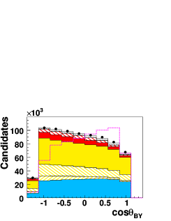
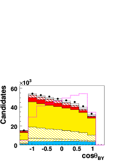
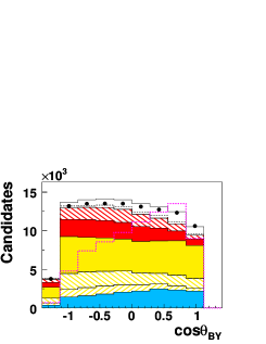
If a Y𝑌Y candidate originates from a signal decay mode, the cosine of the angle between the momentum vectors of the B𝐵B meson and the Y𝑌Y candidate, cosθBYsubscript𝜃𝐵𝑌\cos\theta_{BY}, can be calculated as follows,

cosθBY=2EBEYMB2MY22pBpY,subscript𝜃BY2subscriptsuperscript𝐸𝐵subscriptsuperscript𝐸𝑌superscriptsubscript𝑀𝐵2superscriptsubscript𝑀𝑌22subscriptsuperscript𝑝𝐵subscriptsuperscript𝑝𝑌\cos\theta_{\rm BY}={\frac{2E^{*}_{B}E^{*}_{Y}-M_{B}^{2}-M_{Y}^{2}}{2p^{*}_{B}\ p^{*}_{Y}}}, (14)

and the condition |cosθBY|1.0subscript𝜃BY1.0|\cos\theta_{\rm BY}|\leq 1.0 should be fulfilled. The energy EBsubscriptsuperscript𝐸𝐵E^{*}_{B} and momentum pBsubscriptsuperscript𝑝𝐵p^{*}_{B} of the B𝐵B meson are not measured event-by-event. Specifically, EB=s/2subscriptsuperscript𝐸𝐵𝑠2E^{*}_{B}=\sqrt{s}/2 is given by the average c.m. energy of the colliding beams, and the B𝐵B momentum is derived as pB=EB2MB2subscriptsuperscript𝑝𝐵subscriptsuperscript𝐸absent2𝐵subscriptsuperscript𝑀2𝐵p^{*}_{B}=\sqrt{E^{*2}_{B}-M^{2}_{B}}. To allow for the finite resolution in this variable, we impose the requirement 1.2<cosθBY<1.11.2subscript𝜃BY1.1-1.2<\cos\theta_{\rm BY}<1.1.

IV.1.2 Neutrino Reconstruction

The neutrino four-momentum, Pν(Emiss,pmiss)similar-to-or-equalssubscript𝑃𝜈subscript𝐸misssubscript𝑝missP_{\nu}\simeq(E_{\mathrm{miss}},\vec{p}_{\mathrm{miss}}), is inferred from the difference between the net four-momentum of the colliding-beam particles, Pe+e=(Ee+e,pe+e)subscript𝑃superscript𝑒superscript𝑒subscript𝐸superscript𝑒superscript𝑒subscript𝑝superscript𝑒superscript𝑒P_{e^{+}e^{-}}=(E_{e^{+}e^{-}},\vec{p}_{e^{+}e^{-}}), and the sum of the measured four-vectors of all detected particles in the event,

(Emiss,pmiss)=(Ee+e,pe+e)(iEi,ipi),subscript𝐸misssubscript𝑝misssubscript𝐸superscript𝑒superscript𝑒subscript𝑝superscript𝑒superscript𝑒subscript𝑖subscript𝐸𝑖subscript𝑖subscript𝑝𝑖(E_{\mathrm{miss}},\vec{p}_{\mathrm{miss}})=(E_{e^{+}e^{-}},\vec{p}_{e^{+}e^{-}})-(\sum_{i}E_{i},\sum_{i}\vec{p}_{i}), (15)

where Eisubscript𝐸𝑖E_{i} and pisubscript𝑝𝑖\vec{p}_{i} are the energy and three-momentum of the ithsuperscript𝑖thi^{\rm th} track or EMC shower, measured in the laboratory frame. The energy calculation depends on the correct mass assignments for charged tracks. For this reason we choose to calculate the missing momentum and energy in the laboratory frame rather than in the rest frame of the Υ(4S)Υ4𝑆\mathchar 28935\relax{(4S)}. By doing so, we keep this uncertainty confined to the missing energy.

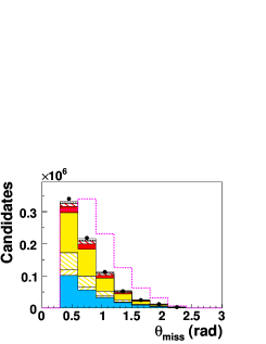
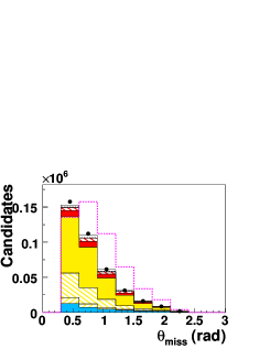
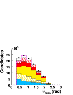
If all particles in the event, except the neutrino, are well measured, Pν(Emiss,pmiss)similar-to-or-equalssubscript𝑃𝜈subscript𝐸misssubscript𝑝missP_{\nu}\simeq(E_{\mathrm{miss}},\vec{p}_{\mathrm{miss}}) is a good approximation. However, particles that are undetected because of inefficiency or acceptance losses, in particular KLsubscript𝐾𝐿K_{L} mesons and additional neutrinos, or spurious tracks or photons that do not originate from the BB¯𝐵¯𝐵B\kern 1.79993pt\overline{\kern-1.79993ptB}{} event, impact the accuracy of this approximation. To reduce the effect of losses due to the limited detector acceptance, we require that the polar angle of the missing momentum in the laboratory frame be in the range 0.3<θmiss<2.2rad0.3subscript𝜃m𝑖𝑠𝑠2.2rad0.3<\theta_{\mathrm{m}iss}<2.2\rm\,rad. We also require the missing momentum in the laboratory frame to exceed 0.5GeV0.5GeV0.5\mathrm{\,Ge\kern-1.00006ptV}.

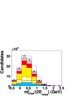
For the rejection of background events and signal decays that are poorly reconstructed as well as events with more than one missing particle, we make use of the missing mass squared of the whole event,

Pν2mmiss2=Emiss2|pmiss|2.similar-to-or-equalssuperscriptsubscript𝑃𝜈2superscriptsubscript𝑚miss2superscriptsubscript𝐸miss2superscriptsubscript𝑝miss2P_{\nu}^{2}\simeq m_{\rm miss}^{2}=E_{\rm miss}^{2}-|\vec{p}_{\mathrm{miss}}|^{2}. (16)

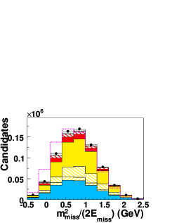
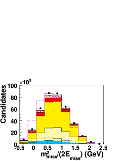
For a correctly reconstructed event with a single semileptonic B𝐵B decay, mmiss2superscriptsubscript𝑚miss2m_{\rm miss}^{2} should be consistent with zero within measurement errors. Failure to detect one or more particles in the event creates a substantial tail at large positive values. Since the resolution in mmiss2superscriptsubscript𝑚miss2m_{\rm miss}^{2} increases linearly with Emisssubscript𝐸missE_{\rm miss}, we use the variable mmiss2/2EmissEmisspmisssimilar-to-or-equalssuperscriptsubscript𝑚miss22subscript𝐸misssubscript𝐸misssubscript𝑝missm_{\rm miss}^{2}/2E_{\rm miss}\simeq E_{\rm miss}-p_{\mathrm{miss}} as a discriminator and require mmiss2/2Emiss<2.5GeVsuperscriptsubscript𝑚miss22subscript𝐸miss2.5GeVm_{\rm miss}^{2}/2E_{\rm miss}<2.5\mathrm{\,Ge\kern-1.00006ptV}.

IV.1.3 Variables Used for Signal Extraction

The kinematic consistency of the candidate decay with a signal B𝐵B decay is ascertained using two variables, the beam-energy substituted B𝐵B mass mESsubscript𝑚ESm_{\rm ES}, and the difference between the reconstructed and expected energy of the B𝐵B candidate ΔEΔ𝐸\Delta E. In the laboratory frame, they are defined as

ΔE=PBPe+es/2sΔ𝐸subscript𝑃𝐵subscript𝑃superscript𝑒superscript𝑒𝑠2𝑠\Delta E=\frac{P_{B}\cdot P_{e^{+}e^{-}}-s/2}{\sqrt{s}} (17)

and

mES=(s/2+pBpe+e)2Ee+e2pB2,subscript𝑚ESsuperscript𝑠2subscript𝑝𝐵subscript𝑝superscript𝑒superscript𝑒2superscriptsubscript𝐸superscript𝑒superscript𝑒2superscriptsubscript𝑝𝐵2m_{\rm ES}=\sqrt{\frac{(s/2+\vec{p}_{B}\cdot\vec{p}_{e^{+}e^{-}})\,^{2}}{E_{e^{+}e^{-}}^{2}}-p_{B}^{2}}\ , (18)

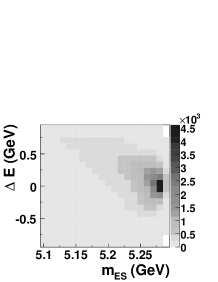
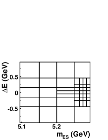
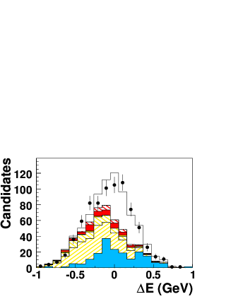
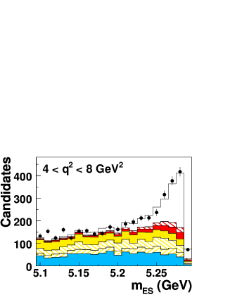
where PB=(EB,pB)subscript𝑃𝐵subscript𝐸𝐵subscript𝑝𝐵P_{B}=(E_{B},\vec{p}_{B}) and Pe+esubscript𝑃superscript𝑒superscript𝑒P_{e^{+}e^{-}} denote the four-momenta of the B𝐵B meson and the colliding beam particles, respectively. The B𝐵B-meson momentum vector pBsubscript𝑝𝐵\vec{p}_{B} is determined from the measured three-momenta of the decay products, and Pe+esubscript𝑃superscript𝑒superscript𝑒P_{e^{+}e^{-}} is derived from the calibration and monitoring of the energies and angles of the stored beams. We extract the signal yields by a fit to the two-dimensional ΔEmESΔ𝐸subscript𝑚ES\Delta E-\mbox{$m_{\rm ES}$} distributions in bins of the momentum transfer squared q2superscript𝑞2q^{2}. We define a region in the ΔEmESΔ𝐸subscript𝑚ES\Delta E-\mbox{$m_{\rm ES}$} plane that contains almost all of the signal events and leaves sufficient phase space to constrain the different background contributions. This 𝑓𝑖𝑡𝑟𝑒𝑔𝑖𝑜𝑛𝑓𝑖𝑡𝑟𝑒𝑔𝑖𝑜𝑛\it{fit\,region} is defined as

|ΔE|<0.95GeV, 5.095<mES<5.295GeV.formulae-sequenceΔ𝐸0.95GeV5.095subscript𝑚ES5.295GeV|\Delta E|<0.95\mathrm{\,Ge\kern-1.00006ptV}\ ,\ 5.095<m_{\rm ES}<5.295\mathrm{\,Ge\kern-1.00006ptV}. (19)

Only candidates that fall inside the fit region are considered in the analysis. We also define a smaller region where the signal contribution is much enhanced relative to the background. This 𝑠𝑖𝑔𝑛𝑎𝑙𝑟𝑒𝑔𝑖𝑜𝑛𝑠𝑖𝑔𝑛𝑎𝑙𝑟𝑒𝑔𝑖𝑜𝑛\it{signal\,region} is defined as

0.15<ΔE<0.25GeV, 5.255<mES<5.295GeV.formulae-sequence0.15Δ𝐸0.25GeV5.255subscript𝑚ES5.295GeV-0.15<\Delta E<0.25\mathrm{\,Ge\kern-1.00006ptV}\ ,\ 5.255<m_{\rm ES}<5.295\mathrm{\,Ge\kern-1.00006ptV}. (20)

The signal region is chosen to be slightly asymmetric in ΔEΔ𝐸\Delta E to avoid sizable BXcν𝐵subscript𝑋𝑐𝜈B\rightarrow X_{c}\ell\nu background, which peaks near 0.2GeV0.2GeV-0.2\mathrm{\,Ge\kern-1.00006ptV}. In the following, we refer to the phase space outside the signal region, but inside the fit region, as the side bands.

As a measure of the momentum transfer squared q2superscript𝑞2q^{2} we adopt the mass squared of the virtual W𝑊W, i.e., the invariant mass squared of the four-vector sum of the reconstructed lepton and neutrino,

qraw2=[(E,p)+(Emiss,pmiss)]2.subscriptsuperscript𝑞2rawsuperscriptdelimited-[]subscript𝐸subscript𝑝subscript𝐸misssubscript𝑝miss2q^{2}_{\rm raw}=[(E_{\ell},\vec{p}_{\ell})+(E_{\mathrm{miss}},\vec{p}_{\mathrm{miss}})]^{2}. (21)

The resolution in qraw2subscriptsuperscript𝑞2rawq^{2}_{\rm raw} is dominated by the measurement of the missing energy which tends to have a poorer resolution than the measured missing momentum, because the missing momentum is a vector sum and contributions from particle losses (or additional tracks and EMC showers) do not add linearly as is the case for Emisssubscript𝐸missE_{\rm miss}. Thus for the definition of qraw2subscriptsuperscript𝑞2rawq^{2}_{\rm raw} it is advantageous to replace Emisssubscript𝐸missE_{\mathrm{miss}} by pmisssubscript𝑝missp_{\mathrm{miss}}, the absolute value of the measured missing momentum,

qraw2=[(E,p)+(pmiss,pmiss)]2.subscriptsuperscript𝑞2rawsuperscriptdelimited-[]subscript𝐸subscript𝑝subscript𝑝misssubscript𝑝miss2q^{2}_{\rm raw}=[(E_{\ell},\vec{p}_{\ell})+(p_{\mathrm{miss}},\vec{p}_{\mathrm{miss}})]^{2}. (22)

The resolution of qraw2subscriptsuperscript𝑞2rawq^{2}_{\rm raw} can be further improved by scaling pmisssubscript𝑝missp_{\mathrm{miss}} by a factor of α𝛼\alpha, such that ΔEΔ𝐸\Delta E of the B𝐵B candidate is forced to zero,

pν=αpmisswithα=1ΔEEmiss,formulae-sequencesubscript𝑝𝜈𝛼subscript𝑝misswith𝛼1Δ𝐸subscript𝐸miss\vec{p}_{\nu}=\alpha\vec{p}_{\mathrm{miss}}\quad\mbox{with}\ \alpha=1-\frac{\Delta E}{E_{\rm miss}}\ , (23)

and substituting pνsubscript𝑝𝜈\vec{p}_{\nu} for pmisssubscript𝑝miss\vec{p}_{\mathrm{miss}} to obtain qcorr2subscriptsuperscript𝑞2corrq^{2}_{\mathrm{corr}}. Any candidates for which this q2superscript𝑞2q^{2} correction yields unphysical values, qcorr2<0GeV2subscriptsuperscript𝑞2corr0superscriptGeV2q^{2}_{\mathrm{corr}}<0\mathrm{\,Ge\kern-1.00006ptV}^{2}, are rejected. This is the case for about 1%percent11\% of the background not associated with semileptonic decays. The quantity qcorr2subscriptsuperscript𝑞2corrq^{2}_{\mathrm{corr}} is used as the measured q2superscript𝑞2q^{2} throughout this analysis.

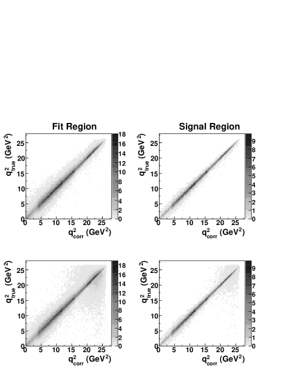
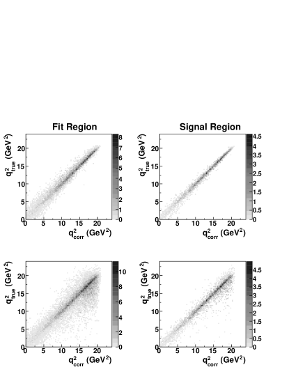
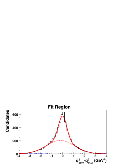
The q2superscript𝑞2q^{2} resolution is critical for the measurements of the form factors. Figure 4 shows the correlation between the true q2superscript𝑞2q^{2} and the reconstructed qcorr2subscriptsuperscript𝑞2corrq^{2}_{\rm corr} for simulated samples of Bπν𝐵𝜋𝜈B\rightarrow\pi\ell\nu and Bρν𝐵𝜌𝜈B\rightarrow\rho\ell\nu candidates passing the entire event selection, which is described below. Correctly reconstructed signal events and combinatorial signal events, for which the hadron has been incorrectly selected, are shown. For correctly reconstructed signal decays the resolution improves with higher q2superscript𝑞2q^{2} and can be well described by the sum of two Gaussian resolution functions, see Table 4. In the signal region, the widths of the core resolution are in the range 0.180.34GeV20.180.34superscriptGeV20.18-0.34\mathrm{\,Ge\kern-1.00006ptV}^{2}, and the tails can be approximated by a second Gaussian function with widths in the range 0.60.8GeV20.60.8superscriptGeV20.6-0.8\mathrm{\,Ge\kern-1.00006ptV}^{2}. As expected, the resolution is significantly worse in the larger fit region. Combinatorial signal events contribute primarily at high q2superscript𝑞2q^{2}. We rely on the Monte Carlo simulation to reproduce the resolution in the reconstructed qcorr2subscriptsuperscript𝑞2corrq^{2}_{\rm corr} variable.

Refer to caption
Refer to caption
Refer to caption
Refer to caption
Figure 4: q2superscript𝑞2q^{2} resolution for B0π+νsuperscript𝐵0superscript𝜋superscript𝜈B^{0}\rightarrow\pi^{-}\ell^{+}\nu (left) and B0ρ+νsuperscript𝐵0superscript𝜌superscript𝜈B^{0}\rightarrow\rho^{-}\ell^{+}\nu (right) samples after the full event selection: two-dimensional distribution of qtrue2subscriptsuperscript𝑞2trueq^{2}_{\mathrm{true}} versus qcorr2subscriptsuperscript𝑞2corrq^{2}_{\mathrm{corr}} in the fit region and in the signal region. Top row: true signal decays, middle row: all signal decays (true and combinatorial), bottom row: distribution of qcorr2qtrue2subscriptsuperscript𝑞2corrsubscriptsuperscript𝑞2trueq^{2}_{\mathrm{corr}}-q^{2}_{\mathrm{true}} for true signal (black, solid histogram) and combinatorial signal (blue, dashed histogram) in the fit region. The fit of the sum of two Gaussian functions to the true signal distribution is shown as a solid red line, the contribution of the broader of the two functions is shown as a dotted red line.
Table 4: Description of the q2superscript𝑞2q^{2} resolution in terms of a sum of two Gaussian resolution functions for true signal decays in the ΔEmESΔ𝐸subscript𝑚ES\Delta E-m_{\rm ES} fit region and in the signal region, integrated over q2superscript𝑞2q^{2}; σ1subscript𝜎1\sigma_{1}, μ1subscript𝜇1\mu_{1} and σ2subscript𝜎2\sigma_{2}, μ2subscript𝜇2\mu_{2} denote the means and the widths of the two Gaussian functions, and the last column lists the fraction of the events characterized by the narrower resolution function.
Gaussian Fct. 1 Gaussian Fct. 2
Signal mode μ1subscript𝜇1\mu_{1}(GeV2superscriptGeV2\mathrm{\,Ge\kern-1.00006ptV}^{2}) σ1subscript𝜎1\sigma_{1}(GeV2superscriptGeV2\mathrm{\,Ge\kern-1.00006ptV}^{2}) μ2subscript𝜇2\mu_{2}(GeV2superscriptGeV2\mathrm{\,Ge\kern-1.00006ptV}^{2}) σ2subscript𝜎2\sigma_{2}(GeV2superscriptGeV2\mathrm{\,Ge\kern-1.00006ptV}^{2}) Fraction
Fit region B0π+νsuperscript𝐵0superscript𝜋superscript𝜈B^{0}\rightarrow\pi^{-}\ell^{+}\nu -0.005 0.380 -0.021 1.270 0.35
B+π0+νsuperscript𝐵superscript𝜋0superscript𝜈B^{+}\rightarrow\pi^{0}\ell^{+}\nu 0.076 0.468 -0.039 1.343 0.43
B0ρ+νsuperscript𝐵0superscript𝜌superscript𝜈B^{0}\rightarrow\rho^{-}\ell^{+}\nu 0.005 0.343 -0.386 1.094 0.45
B+ρ0+νsuperscript𝐵superscript𝜌0superscript𝜈B^{+}\rightarrow\rho^{0}\ell^{+}\nu -0.032 0.311 -0.498 1.086 0.46
Signal region B0π+νsuperscript𝐵0superscript𝜋superscript𝜈B^{0}\rightarrow\pi^{-}\ell^{+}\nu 0.006 0.242 -0.020 0.720 0.45
B+π0+νsuperscript𝐵superscript𝜋0superscript𝜈B^{+}\rightarrow\pi^{0}\ell^{+}\nu 0.058 0.338 0.172 0.807 0.58
B0ρ+νsuperscript𝐵0superscript𝜌superscript𝜈B^{0}\rightarrow\rho^{-}\ell^{+}\nu 0.042 0.246 0.036 0.647 0.50
B+ρ0+νsuperscript𝐵superscript𝜌0superscript𝜈B^{+}\rightarrow\rho^{0}\ell^{+}\nu 0.010 0.177 -0.078 0.586 0.46

IV.2 Background Suppression

IV.2.1 Signal and Background Sources

A variety of processes contribute to the four samples of selected candidates for the charmless semileptonic decay modes B0π+νsuperscript𝐵0superscript𝜋superscript𝜈B^{0}\rightarrow\pi^{-}\ell^{+}\nu, B+π0+νsuperscript𝐵superscript𝜋0superscript𝜈B^{+}\rightarrow\pi^{0}\ell^{+}\nu, B0ρ+νsuperscript𝐵0superscript𝜌superscript𝜈B^{0}\rightarrow\rho^{-}\ell^{+}\nu, and B+ρ0+νsuperscript𝐵superscript𝜌0superscript𝜈B^{+}\rightarrow\rho^{0}\ell^{+}\nu. We divide the signal and background for each of the four candidate samples into a set of sources based on the origin of the charged lepton candidate.

  • Signal:  We differentiate four classes of signal events; for all of them the lepton originates from a signal decay under study:

    • True signal:    the hadron originates from the signal decay under study;

    • Combinatorial Signal:    the hadron is incorrectly selected, in many cases from decay products of the second B𝐵B meson in the event;

    • Isospin-conjugate signal:    the lepton originates from the isospin conjugate of the signal decay;

    • Cross-feed signal:    the lepton originates from another signal decay mode, for instance Bρν𝐵𝜌𝜈B\rightarrow\rho\ell\nu in a Bπν𝐵𝜋𝜈B\rightarrow\pi\ell\nu sample.

  • Continuum background:  We differentiate two classes of continuum backgrounds:

    • True leptons:   the lepton candidate originates from a leptonic or semileptonic decay of a hadron produced in e+eqq¯superscript𝑒superscript𝑒𝑞¯𝑞e^{+}e^{-}\rightarrow q\overline{q} (mostly cc¯𝑐¯𝑐c\overline{c}) or e+e+(γ)superscript𝑒superscript𝑒superscriptsuperscript𝛾e^{+}e^{-}\rightarrow\ell^{+}\ell^{-}(\gamma) processes, where +superscriptsuperscript\ell^{+}\ell^{-} stands for e+e,μ+μsuperscript𝑒superscript𝑒superscript𝜇superscript𝜇e^{+}e^{-},\mu^{+}\mu^{-} or τ+τsuperscript𝜏superscript𝜏\tau^{+}\tau^{-}, or e+eγγsuperscript𝑒superscript𝑒𝛾𝛾e^{+}e^{-}\rightarrow\gamma\gamma;

    • Fake leptons:   the lepton candidate is a misidentified hadron; this is a sizable contribution to the muon sample.

  • BXuν𝐵subscript𝑋𝑢𝜈B\rightarrow X_{u}\ell\nu background:  We differentiate two different sources of BXuν𝐵subscript𝑋𝑢𝜈B\rightarrow X_{u}\ell\nu background:

    • Exclusive BXuν𝐵subscript𝑋𝑢𝜈B\rightarrow X_{u}\ell\nu decays involving a single hadron with mass below 1 GeVGeV\mathrm{\,Ge\kern-1.00006ptV}:   decays that are not analyzed as signal (B+ω+νsuperscript𝐵𝜔superscript𝜈B^{+}\rightarrow\omega\ell^{+}\nu, B+η+νsuperscript𝐵𝜂superscript𝜈B^{+}\rightarrow\eta\ell^{+}\nu, and B+η+νsuperscript𝐵superscript𝜂superscript𝜈B^{+}\rightarrow\eta^{\prime}\ell^{+}\nu) ;

    • Inclusive BXuν𝐵subscript𝑋𝑢𝜈B\rightarrow X_{u}\ell\nu decays:    decays involving more than one hadron or a single hadron with mass above 1 GeVGeV\mathrm{\,Ge\kern-1.00006ptV}.

  • BB¯𝐵¯𝐵B\kern 1.79993pt\overline{\kern-1.79993ptB}{} background:  We differentiate three classes of BB¯𝐵¯𝐵B\kern 1.79993pt\overline{\kern-1.79993ptB}{} background, excluding BXuν𝐵subscript𝑋𝑢𝜈B\rightarrow X_{u}\ell\nu decays:

    • Primary leptons, i.e., BXcν𝐵subscript𝑋𝑐𝜈B\rightarrow X_{c}\ell\nu decays:    the lepton originates from a charm semileptonic B𝐵B decay, either BDν𝐵𝐷𝜈B\rightarrow D\ell\nu, BDν𝐵superscript𝐷𝜈B\rightarrow D^{*}\ell\nu, or BD()(nπ)ν𝐵superscript𝐷𝑛𝜋𝜈B\rightarrow D^{(*)}(n\pi)\ell\nu with n1𝑛1n\geq 1 additional pions; this class is dominated by BDν𝐵superscript𝐷𝜈B\rightarrow D^{*}\ell\nu decays; the largest contributions involve hadrons that do not originate from the semileptonic decay;

    • Secondary leptons:    the lepton originates from the decay of a particle other than a B𝐵B meson, for instance charm mesons, τ𝜏\tau leptons, J/ψ𝐽𝜓{J\mskip-3.0mu/\mskip-2.0mu\psi\mskip 2.0mu}, or from photon conversions;

    • Fake leptons:    the lepton candidate is not a lepton, but a misidentified charged hadron; this background is dominated by fake muons.

    Given that the secondary-lepton and fake-lepton BB¯𝐵¯𝐵B\kern 1.79993pt\overline{\kern-1.79993ptB}{} background contributions are relatively small in this analysis, we combine them into one class (other BB¯𝐵¯𝐵B\kern 1.79993pt\overline{\kern-1.79993ptB}{}).

For intermediate values of q2superscript𝑞2q^{2} (in the range 4<q2<20GeV24superscript𝑞220superscriptGeV24<q^{2}<20\mathrm{\,Ge\kern-1.00006ptV}^{2}), BXcν𝐵subscript𝑋𝑐𝜈B\rightarrow X_{c}\ell\nu decays are by far the dominant background, whereas continuum background contributes mostly at low and high q2superscript𝑞2q^{2}. The BXuν𝐵subscript𝑋𝑢𝜈B\rightarrow X_{u}\ell\nu decays have much smaller branching fractions, but their properties are very similar to the signal decays and thus they are difficult to discriminate against. They contribute mostly at high q2superscript𝑞2q^{2}, where they are the dominant background.

IV.2.2 Neural Networks

To separate signal events from the background sources, continuum events, non-signal BXuν𝐵subscript𝑋𝑢𝜈B\rightarrow X_{u}\ell\nu decays and the remaining BB¯𝐵¯𝐵B\kern 1.79993pt\overline{\kern-1.79993ptB}{} events, we employ a neural-network technique based on a multi-layer perceptron (MLP) MLP . We have set up a network structure with seven input neurons and one hidden layer with three neurons and have adopted the method introduced by Broyden, Fletcher, Goldfarb, and Shanno BFGS to train the network. Some of the input variables are used as part of the event preselection that is designed to reduce the BB¯𝐵¯𝐵B\kern 1.79993pt\overline{\kern-1.79993ptB}{} and continuum backgrounds by cutting out regions where the signal contribution is small or where there are spikes in distributions, which the neural network may not deal with effectively. The following variables are input to the neural networks:

  • R2𝑅2R2, the second normalized Fox-Wolfram moment Fox-wolfram determined from all charged and neutral particles in the event; we require R2<0.5𝑅20.5R2<0.5;

  • L2=ipicos2θi𝐿2subscript𝑖subscriptsuperscript𝑝𝑖superscript2subscriptsuperscript𝜃𝑖L2=\sum_{i}p^{*}_{i}{\cos}^{2}\theta^{*}_{i}, where the sum runs over all tracks in the event excluding the Y𝑌Y candidate, and pisubscriptsuperscript𝑝𝑖p^{*}_{i} and θisubscriptsuperscript𝜃𝑖\theta^{*}_{i} refer to the c.m. momenta and the angles measured with respect to the thrust axis of the Y𝑌Y candidate; we set a loose restriction, L2<3.0𝐿23.0L2<3.0 GeVGeV\mathrm{\,Ge\kern-1.00006ptV}.

  • cosΔθthrustΔsubscript𝜃thrust\cos\Delta\theta_{\rm thrust}, where ΔθthrustΔsubscript𝜃thrust\Delta\theta_{\rm thrust} is the angle between the thrust axis of the Y𝑌Y candidate and thrust axis of all other detected particles in the event; there is no preselection requirement for this variable;

  • mmiss2/(2Emiss)=(Emiss2pmiss2)/(2Emiss)superscriptsubscript𝑚miss22subscript𝐸misssuperscriptsubscript𝐸miss2superscriptsubscript𝑝miss22subscript𝐸missm_{\rm miss}^{2}/(2E_{\rm miss})=(E_{\rm miss}^{2}-p_{\rm miss}^{2})/(2E_{\rm miss}); we require |mmiss2/2Emiss|<2.5GeVsuperscriptsubscript𝑚miss22subscript𝐸miss2.5GeV|m_{\rm miss}^{2}/2E_{\rm miss}|<2.5~{}\mathrm{\,Ge\kern-1.00006ptV};

  • cosθBYsubscript𝜃BY\cos\theta_{\rm BY}; we require 1.2<cosθBY<1.11.2subscript𝜃BY1.1-1.2<\cos\theta_{\rm BY}<1.1;

  • cosθWsubscript𝜃𝑊\cos\theta_{W\ell}, the helicity angle of the lepton; we require |cosθW|<0.8subscript𝜃𝑊0.8|\cos\theta_{W\ell}|<0.8 for the B0π+νsuperscript𝐵0superscript𝜋superscript𝜈B^{0}\rightarrow\pi^{-}\ell^{+}\nu and B+π0+νsuperscript𝐵superscript𝜋0superscript𝜈B^{+}\rightarrow\pi^{0}\ell^{+}\nu modes;

  • θmisssubscript𝜃miss\theta_{\rm miss}, the polar angle of the missing momentum in the laboratory frame; we require 0.3<θmiss<2.20.3subscript𝜃miss2.20.3<\theta_{\rm miss}<2.2 rad.

The first three input variables are sensitive to the topological difference between the jet-like continuum events and the more spherical BB¯𝐵¯𝐵B\kern 1.79993pt\overline{\kern-1.79993ptB}{} events. Restrictions on these variables do not bias the q2superscript𝑞2q^{2} distribution significantly.

The restrictions placed on cosθBYsubscript𝜃BY\cos\theta_{\rm BY}, mmiss2/(2Emiss)superscriptsubscript𝑚miss22subscript𝐸missm_{\rm miss}^{2}/(2E_{\rm miss}), and θmisssubscript𝜃miss\theta_{\rm miss} do not significantly bias the q2superscript𝑞2q^{2} distribution either. However, the variable cosθWsubscript𝜃𝑊\cos\theta_{W\ell} is correlated with the lepton momentum and thereby q2superscript𝑞2q^{2}. To ensure that the selection does not adversely affect the measurement of the q2superscript𝑞2q^{2} spectrum, we have chosen rather moderate restrictions on cosθWsubscript𝜃𝑊\cos\theta_{W\ell}.

Figure 5 shows the ΔEΔ𝐸\Delta E and mESsubscript𝑚ESm_{\rm ES} distributions for samples of B0π+νsuperscript𝐵0superscript𝜋superscript𝜈B^{0}\rightarrow\pi^{-}\ell^{+}\nu and B0ρ+νsuperscript𝐵0superscript𝜌superscript𝜈B^{0}\rightarrow\rho^{-}\ell^{+}\nu candidates (integrated over q2superscript𝑞2q^{2}) that have been preselected by the criteria described above. The stacked histograms show the signal and background contributions compared to the data, prior to the fit. The three dominant backgrounds are BXcν𝐵subscript𝑋𝑐𝜈B\rightarrow X_{c}\ell\nu decays (including BDν𝐵𝐷𝜈B\rightarrow D\ell\nu, BDν𝐵superscript𝐷𝜈B\rightarrow D^{*}\ell\nu and BD()(nπ)ν𝐵superscript𝐷𝑛𝜋𝜈B\rightarrow D^{(*)}(n\pi)\ell\nu), qq¯𝑞¯𝑞q\bar{q} continuum and BXuν𝐵subscript𝑋𝑢𝜈B\rightarrow X_{u}\ell\nu decays. The signal contributions are very small by comparison and difficult to observe.
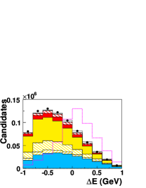
Refer to caption
Refer to caption
Refer to caption
Refer to caption
Refer to caption
Refer to caption
Figure 5: (color online) Distributions of ΔEΔ𝐸\Delta E and mESsubscript𝑚ESm_{\rm ES} for B0π+νsuperscript𝐵0superscript𝜋superscript𝜈B^{0}\rightarrow\pi^{-}\ell^{+}\nu (left) and B0ρ+νsuperscript𝐵0superscript𝜌superscript𝜈B^{0}\rightarrow\rho^{-}\ell^{+}\nu (right) candidates after the preselection, i.e., prior to the neural-network application. The stacked histograms show the predicted signal and background contributions prior to the fit. The expected signal distribution (with arbitrary normalization) is indicated as a magenta dashed histogram.

The neural networks are trained separately for the three background categories and for different q2superscript𝑞2q^{2} intervals. We introduce six bins in q2superscript𝑞2q^{2} for Bπν𝐵𝜋𝜈B\rightarrow\pi\ell\nu and three bins for Bρν𝐵𝜌𝜈B\rightarrow\rho\ell\nu. The bin sizes are 4GeV24superscriptGeV24\mathrm{\,Ge\kern-1.00006ptV}^{2} for Bπν𝐵𝜋𝜈B\rightarrow\pi\ell\nu and 8GeV28superscriptGeV28\mathrm{\,Ge\kern-1.00006ptV}^{2} for Bρν𝐵𝜌𝜈B\rightarrow\rho\ell\nu, except for the last bin, which extends to the kinematic limit of 26.4GeV226.4superscriptGeV226.4\mathrm{\,Ge\kern-1.00006ptV}^{2} and 20.3GeV220.3superscriptGeV220.3\mathrm{\,Ge\kern-1.00006ptV}^{2}, respectively. Thus in total we train 3×(2×6+2×3)=5432623543\times(2\times 6+2\times 3)=54 neural networks. Since we aim for a good signal-to-background ratio in the region where most of the signal is located, we do not train the neural network with events in the whole fit region, but in an extended signal region, 0.25<ΔE<0.35GeV,5.240<mES<5.295GeVformulae-sequence0.25Δ𝐸0.35GeV5.240subscript𝑚ES5.295GeV-0.25<\Delta E<0.35\mathrm{\,Ge\kern-1.00006ptV},5.240<m_{\rm ES}<5.295\mathrm{\,Ge\kern-1.00006ptV}.

For the training of the neural networks we use MC simulated events containing correctly reconstructed signal decays and the following simulated background samples:

  1. 1.

    a sample of continuum events, e+eqq¯superscript𝑒superscript𝑒𝑞¯𝑞e^{+}e^{-}\rightarrow q\overline{q} with q=u,d,s,c𝑞𝑢𝑑𝑠𝑐q=u,d,s,c (qq¯𝑞¯𝑞q\bar{q} neural network);

  2. 2.

    a combined sample of BXcν𝐵subscript𝑋𝑐𝜈B\rightarrow X_{c}\ell\nu decays (BXcν𝐵subscript𝑋𝑐𝜈B\rightarrow X_{c}\ell\nu neural network); and

  3. 3.

    a sample of inclusive BXuν𝐵subscript𝑋𝑢𝜈B\rightarrow X_{u}\ell\nu decays (BXuν𝐵subscript𝑋𝑢𝜈B\rightarrow X_{u}\ell\nu neural network).

The training of the neural networks and the subsequent background reduction is performed sequentially for the three background samples. We use subsamples of typically less than half the total MC samples for training and validation of the neural networks. Of these subsamples, one half of the events is used as training sample, and the other half for validation.

Studies of the neural-network performance for the BXuν𝐵subscript𝑋𝑢𝜈B\rightarrow X_{u}\ell\nu background indicate that the separation of this background from the signal is very difficult because of the similarity in the shape of the distributions, especially for the B+π0+νsuperscript𝐵superscript𝜋0superscript𝜈B^{+}\rightarrow\pi^{0}\ell^{+}\nu and the Bρν𝐵𝜌𝜈B\rightarrow\rho\ell\nu samples. Given these difficulties, we use the BXuν𝐵subscript𝑋𝑢𝜈B\rightarrow X_{u}\ell\nu neural network only for the B0π+νsuperscript𝐵0superscript𝜋superscript𝜈B^{0}\rightarrow\pi^{-}\ell^{+}\nu sample, and only for q2>12GeV2superscript𝑞212superscriptGeV2q^{2}>12\mathrm{\,Ge\kern-1.00006ptV}^{2}, where the BXuν𝐵subscript𝑋𝑢𝜈B\rightarrow X_{u}\ell\nu background becomes significant.

Figure 6 shows, for the sample of B0π+νsuperscript𝐵0superscript𝜋superscript𝜈B^{0}\rightarrow\pi^{-}\ell^{+}\nu candidates, the distributions of the seven input variables to the neural networks. The distributions are shown sequentially after application of the preselection, the qq¯𝑞¯𝑞q\bar{q} neural network and the BXcν𝐵subscript𝑋𝑐𝜈B\rightarrow X_{c}\ell\nu neural network to illustrate the change in the sample composition. Figures 7 to 9 show the distributions of the three neural-network discriminators for the B0π+νsuperscript𝐵0superscript𝜋superscript𝜈B^{0}\rightarrow\pi^{-}\ell^{+}\nu sample in four of the six q2superscript𝑞2q^{2} bins. Figures 10 and 11 show the distributions of the two neural-network discriminators for the B0ρ+νsuperscript𝐵0superscript𝜌superscript𝜈B^{0}\rightarrow\rho^{-}\ell^{+}\nu sample in all three q2superscript𝑞2q^{2} bins. The discriminator cuts are chosen to minimize the total error on the signal yield for each channel, using the sum in quadrature of the error obtained from the maximum-likelihood fit described in Section VI and the estimated total systematic error of the partial signal branching fraction in each q2superscript𝑞2q^{2} bin (see Section VII). The data-MC agreement is reasonably good for the input distributions and the neural-network discriminators. One should keep in mind that at this stage the distributions are taken directly from the simulation, without any adjustments or fit.
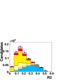
Refer to captionRefer to captionRefer to captionRefer to captionRefer to captionRefer to captionRefer to caption Refer to captionRefer to captionRefer to captionRefer to captionRefer to captionRefer to captionRefer to caption Refer to captionRefer to captionRefer to captionRefer to captionRefer to captionRefer to captionRefer to caption
Figure 6: (color online) Background suppression for B0π+νsuperscript𝐵0superscript𝜋superscript𝜈B^{0}\rightarrow\pi^{-}\ell^{+}\nu candidates. Distributions of the seven input variables to the neural network: after the preselection (left column), after the qq¯𝑞¯𝑞q\bar{q} neural network (center column), and after the BXcν𝐵subscript𝑋𝑐𝜈B\rightarrow X_{c}\ell\nu neural network (right column). The data are compared to the sum of the MC-simulated background contributions; for a legend see Figure 5. The expected signal distribution is overlaid as a magenta, dashed histogram with arbitrary normalization.
Refer to caption
Refer to caption
Refer to caption
Refer to caption
Refer to caption
Refer to caption
Refer to caption
Refer to caption
Figure 7: (color online) The qq¯𝑞¯𝑞q\bar{q} neural-network discriminators for B0π+νsuperscript𝐵0superscript𝜋superscript𝜈B^{0}\rightarrow\pi^{-}\ell^{+}\nu candidates in the signal region, 0.15<|ΔE|<0.25GeV; 5.255<mES<5.295GeVformulae-sequence0.15Δ𝐸0.25GeV5.255subscript𝑚ES5.295GeV-0.15<|\Delta E|<0.25\mathrm{\,Ge\kern-1.00006ptV}\,;\,5.255<m_{\rm ES}<5.295\mathrm{\,Ge\kern-1.00006ptV}. The distributions are shown for four different q2superscript𝑞2q^{2} bins, columns from left to right: 0<q2<4GeV20superscript𝑞24superscriptGeV20<q^{2}<4\mathrm{\,Ge\kern-1.00006ptV}^{2}, 4<q2<8GeV24superscript𝑞28superscriptGeV24<q^{2}<8\mathrm{\,Ge\kern-1.00006ptV}^{2}, 12<q2<16GeV212superscript𝑞216superscriptGeV212<q^{2}<16\mathrm{\,Ge\kern-1.00006ptV}^{2}, q2>20GeV2superscript𝑞220superscriptGeV2q^{2}>20\mathrm{\,Ge\kern-1.00006ptV}^{2}. Top row: Discriminator distributions for signal (magneta, dashed) and qq¯𝑞¯𝑞q\bar{q} background (blue, solid), normalized to the same area. The arrows indicate the chosen cuts. Bottom row: Discriminator distributions for data compared with MC-simulated signal and background contributions. For a legend see Figure 5.
Refer to caption
Refer to caption
Refer to caption
Refer to caption
Refer to caption
Refer to caption
Refer to caption
Refer to caption
Figure 8: (color online) The BXcν𝐵subscript𝑋𝑐𝜈B\rightarrow X_{c}\ell\nu neural-network discriminators for B0π+νsuperscript𝐵0superscript𝜋superscript𝜈B^{0}\rightarrow\pi^{-}\ell^{+}\nu candidates in the signal region, 0.15<|ΔE|<0.25GeV; 5.255<mES<5.295GeVformulae-sequence0.15Δ𝐸0.25GeV5.255subscript𝑚ES5.295GeV-0.15<|\Delta E|<0.25\mathrm{\,Ge\kern-1.00006ptV}\,;\,5.255<m_{\rm ES}<5.295\mathrm{\,Ge\kern-1.00006ptV}. The distributions are shown for four different q2superscript𝑞2q^{2} bins, columns from left to right: 0<q2<4GeV20superscript𝑞24superscriptGeV20<q^{2}<4\mathrm{\,Ge\kern-1.00006ptV}^{2}, 4<q2<8GeV24superscript𝑞28superscriptGeV24<q^{2}<8\mathrm{\,Ge\kern-1.00006ptV}^{2}, 12<q2<16GeV212superscript𝑞216superscriptGeV212<q^{2}<16\mathrm{\,Ge\kern-1.00006ptV}^{2}, q2>20GeV2superscript𝑞220superscriptGeV2q^{2}>20\mathrm{\,Ge\kern-1.00006ptV}^{2}. Top row: Discriminator distributions for signal (magneta, dashed) and BXcν𝐵subscript𝑋𝑐𝜈B\rightarrow X_{c}\ell\nu background (blue, solid), normalized to the same area. The arrows indicate the chosen cuts. Bottom row: Discriminator distributions for data compared with MC-simulated signal and background contributions. For a legend see Figure 5.
Refer to caption
Refer to caption
Refer to caption
Refer to caption
Refer to caption
Refer to caption
Figure 9: (color online) The BXuν𝐵subscript𝑋𝑢𝜈B\rightarrow X_{u}\ell\nu neural-network discriminators for B0π+νsuperscript𝐵0superscript𝜋superscript𝜈B^{0}\rightarrow\pi^{-}\ell^{+}\nu candidates in the signal region, 0.15<|ΔE|<0.25GeV; 5.255<mES<5.295GeVformulae-sequence0.15Δ𝐸0.25GeV5.255subscript𝑚ES5.295GeV-0.15<|\Delta E|<0.25\mathrm{\,Ge\kern-1.00006ptV}\,;\,5.255<m_{\rm ES}<5.295\mathrm{\,Ge\kern-1.00006ptV}. The distributions are shown for the three highest q2superscript𝑞2q^{2} bins, columns from left to right: 12<q2<16GeV212superscript𝑞216superscriptGeV212<q^{2}<16\mathrm{\,Ge\kern-1.00006ptV}^{2}, 16<q2<20GeV216superscript𝑞220superscriptGeV216<q^{2}<20\mathrm{\,Ge\kern-1.00006ptV}^{2}, q2>20GeV2superscript𝑞220superscriptGeV2q^{2}>20\mathrm{\,Ge\kern-1.00006ptV}^{2}. Top row: Discriminator distributions for signal (magneta, dashed) and BXuν𝐵subscript𝑋𝑢𝜈B\rightarrow X_{u}\ell\nu background (blue, solid), normalized to the same area. The arrows indicate the chosen cuts. Bottom row: Discriminator distributions for data compared with MC-simulated signal and background contributions. For a legend see Figure 5.
Refer to caption
Refer to caption
Refer to caption
Refer to caption
Refer to caption
Refer to caption
Figure 10: (color online) The qq¯𝑞¯𝑞q\bar{q} neural-network discriminators for B0ρ+νsuperscript𝐵0superscript𝜌superscript𝜈B^{0}\rightarrow\rho^{-}\ell^{+}\nu candidates in the signal region, 0.15<|ΔE|<0.25GeV; 5.255<mES<5.295GeVformulae-sequence0.15Δ𝐸0.25GeV5.255subscript𝑚ES5.295GeV-0.15<|\Delta E|<0.25\mathrm{\,Ge\kern-1.00006ptV}\,;\,5.255<m_{\rm ES}<5.295\mathrm{\,Ge\kern-1.00006ptV}. The distributions are shown for three different q2superscript𝑞2q^{2} bins, columns from left to right: 0<q2<8GeV20superscript𝑞28superscriptGeV20<q^{2}<8\mathrm{\,Ge\kern-1.00006ptV}^{2}, 8<q2<16GeV28superscript𝑞216superscriptGeV28<q^{2}<16\mathrm{\,Ge\kern-1.00006ptV}^{2}, q2>16GeV2superscript𝑞216superscriptGeV2q^{2}>16\mathrm{\,Ge\kern-1.00006ptV}^{2}. Top row: Discriminator distributions for signal (magneta, dashed) and qq¯𝑞¯𝑞q\bar{q} background (blue, solid), normalized to the same area. The arrows indicate the chosen cuts. Bottom row: Discriminator distributions for data compared with MC-simulated signal and background contributions. For a legend see Figure 5.
Refer to caption
Refer to caption
Refer to caption
Refer to caption
Refer to caption
Refer to caption
Figure 11: (color online) The BXcν𝐵subscript𝑋𝑐𝜈B\rightarrow X_{c}\ell\nu neural-network discriminators for B0ρ+νsuperscript𝐵0superscript𝜌superscript𝜈B^{0}\rightarrow\rho^{-}\ell^{+}\nu candidates in the signal region, 0.15<|ΔE|<0.25GeV; 5.255<mES<5.295GeVformulae-sequence0.15Δ𝐸0.25GeV5.255subscript𝑚ES5.295GeV-0.15<|\Delta E|<0.25\mathrm{\,Ge\kern-1.00006ptV}\,;\,5.255<m_{\rm ES}<5.295\mathrm{\,Ge\kern-1.00006ptV}. The distributions are shown for three different q2superscript𝑞2q^{2} bins, columns from left to right: 0<q2<8GeV20superscript𝑞28superscriptGeV20<q^{2}<8\mathrm{\,Ge\kern-1.00006ptV}^{2}, 8<q2<16GeV28superscript𝑞216superscriptGeV28<q^{2}<16\mathrm{\,Ge\kern-1.00006ptV}^{2}, q2>16GeV2superscript𝑞216superscriptGeV2q^{2}>16\mathrm{\,Ge\kern-1.00006ptV}^{2}. Top row: Discriminator distributions for signal (magneta, dashed) and BXcν𝐵subscript𝑋𝑐𝜈B\rightarrow X_{c}\ell\nu background (blue, solid), normalized to the same area. The arrows indicate the chosen cuts. Bottom row: Discriminator distributions for data compared with MC-simulated signal and background contributions. For a legend see Figure 5.
Table 5: Overview of the selection efficiencies for the four signal decays (true and combinatorial signal combined) and their primary background sources, BXuν𝐵subscript𝑋𝑢𝜈B\rightarrow X_{u}\ell\nu, BXcν𝐵subscript𝑋𝑐𝜈B\rightarrow X_{c}\ell\nu, and non-BB¯𝐵¯𝐵B\kern 1.79993pt\overline{\kern-1.79993ptB}{} background.
Selection Signal Xuνsubscript𝑋𝑢𝜈X_{u}\ell\nu Xcνsubscript𝑋𝑐𝜈X_{c}\ell\nu qq¯𝑞¯𝑞q\bar{q}
Units 102superscript10210^{-2} 103superscript10310^{-3} 104superscript10410^{-4} 105superscript10510^{-5}
B0π+νsuperscript𝐵0superscript𝜋superscript𝜈B^{0}\rightarrow\pi^{-}\ell^{+}\nu
Preselection 18.1 25.6 26.4 19.4
NN qq¯𝑞¯𝑞q\bar{q} 11.6 13.4 18.3 2.6
NN BXcν𝐵subscript𝑋𝑐𝜈B\rightarrow X_{c}\ell\nu 7.8 8.1 3.4 1.3
NN BXuν𝐵subscript𝑋𝑢𝜈B\rightarrow X_{u}\ell\nu 6.8 5.3 2.5 1.0
Signal region 1.8 0.5 0.1 <<0.1
B+π0+νsuperscript𝐵superscript𝜋0superscript𝜈B^{+}\rightarrow\pi^{0}\ell^{+}\nu
Preselection 12.8 20.0 17.4 15.1
NN qq¯𝑞¯𝑞q\bar{q} 8.4 11.3 13.3 2.7
NN BXcν𝐵subscript𝑋𝑐𝜈B\rightarrow X_{c}\ell\nu 5.9 6.6 1.9 1.6
Signal region 1.6 0.5 <<0.1 <<0.1
B0ρ+νsuperscript𝐵0superscript𝜌superscript𝜈B^{0}\rightarrow\rho^{-}\ell^{+}\nu
Preselection 8.9 23.9 35.8 13.2
NN qq¯𝑞¯𝑞q\bar{q} 4.8 11.9 18.5 1.0
NN BXcν𝐵subscript𝑋𝑐𝜈B\rightarrow X_{c}\ell\nu 1.1 1.9 0.3 0.2
Signal region 0.3 0.3 <<0.1 <<0.1
B+ρ0+νsuperscript𝐵superscript𝜌0superscript𝜈B^{+}\rightarrow\rho^{0}\ell^{+}\nu
Preselection 11.1 22.1 30.0 12.6
NN qq¯𝑞¯𝑞q\bar{q} 6.8 12.4 17.7 1.5
NN BXcν𝐵subscript𝑋𝑐𝜈B\rightarrow X_{c}\ell\nu 2.5 3.2 0.7 0.5
Signal region 0.8 0.6 <<0.1 <<0.1

Table 5 shows the selection efficiencies for the four signal samples compared to the efficiencies for the dominant background sources for these samples. The total signal efficiencies are typically 67676-7% for Bπν𝐵𝜋𝜈B\rightarrow\pi\ell\nu decays and roughly 12.512.51-2.5% for Bρν𝐵𝜌𝜈B\rightarrow\rho\ell\nu decays in the fit region. The dominant BB¯𝐵¯𝐵B\kern 1.79993pt\overline{\kern-1.79993ptB}{} and qq¯𝑞¯𝑞q\bar{q} backgrounds are suppressed by factors of order 104superscript10410^{4} and 105superscript10510^{5}, respectively.

IV.2.3 Candidate Multiplicity

After the neural-network selection there are on average 1.14 candidates per event in the B0π+νsuperscript𝐵0superscript𝜋superscript𝜈B^{0}\rightarrow\pi^{-}\ell^{+}\nu sample, 1.46 in the B+π0+νsuperscript𝐵superscript𝜋0superscript𝜈B^{+}\rightarrow\pi^{0}\ell^{+}\nu sample, 1.30 in the B0ρ+νsuperscript𝐵0superscript𝜌superscript𝜈B^{0}\rightarrow\rho^{-}\ell^{+}\nu sample, and 1.17 in the B+ρ0+νsuperscript𝐵superscript𝜌0superscript𝜈B^{+}\rightarrow\rho^{0}\ell^{+}\nu sample. We observe fewer candidates for decay modes without neutral pions in the final state. For all four samples, the observed candidate multiplicity is well reproduced by MC simulation.

In case of multiple candidates for a given decay mode, we select the one with the highest probability of the vertex fit for the Y𝑌Y candidate. Since this is not an option for B+π0+νsuperscript𝐵superscript𝜋0superscript𝜈B^{+}\rightarrow\pi^{0}\ell^{+}\nu decays, we select the photon pair with an invariant mass closest to the π0superscript𝜋0\pi^{0} mass. Simulations of signal events indicate that this procedure selects the correct signal decay in 6065606560-65% of the cases. By this selection we do not allow a single event to contribute more than one candidate to a given decay-mode sample, though we do allow an event to contribute candidates to more than one decay-mode sample.

V Data-Monte Carlo Comparisons

The determination of the number of signal events relies heavily on the MC simulation to correctly describe the distributions for signal and background sources. Therefore a significant effort has been devoted to detailed comparisons of data and MC distributions for samples that have been selected to enhance a given source of background.

V.1 Comparison of Off-Resonance Data with 𝒒𝒒¯𝒒bold-¯𝒒q\overline{q} MC

Though we record data below BB¯𝐵¯𝐵B\kern 1.79993pt\overline{\kern-1.79993ptB}{} threshold (off-resonance data) the total luminosity of this sample is only about 10% of the Υ(4S)Υ4𝑆\mathchar 28935\relax{(4S)} data sample (on-resonance data), and thus we need to rely on MC simulation to predict the shapes of these background distributions.

To study the simulation of qq¯𝑞¯𝑞q\overline{q} events, we scale the MC sample to match the integrated luminosity of the off-resonance data. The study is performed separately for samples with electrons and muons. This background contains events with true leptons from leptonic or semileptonic decays of hadrons, as well as hadrons misidentified as leptons. The muon sample is dominated by misidentified hadrons, whereas the electron sample contains small contributions from Dalitz pairs and photon conversions, as well as some residual background from non-qq¯𝑞¯𝑞q\overline{q} processes. We observe a clear difference in the normalization, not only in the relatively small event sample passing the neural-network selection, but also for the much larger sample available before the neural-network suppression. To correct for this difference, we apply additional scale factors to the simulated qq¯𝑞¯𝑞q\overline{q} samples; they are different for electrons and muons.

In addition to correcting the normalization, we also examine the shapes of the mESsubscript𝑚ESm_{\rm ES}, ΔEΔ𝐸\Delta E, and q2superscript𝑞2q^{2} distributions that are used to extract the signal yield. Since the size of the off-resonance data set is small, we study samples with a looser selection, namely we bypass the qq¯𝑞¯𝑞q\bar{q} neural-network discrimination. The comparison of these qq¯𝑞¯𝑞q\bar{q}-enriched samples reveals small differences between data and simulation. We derive linear corrections from the bin-by-bin ratios and apply these corrections to the mESsubscript𝑚ESm_{\rm ES}, ΔEΔ𝐸\Delta E, and q2superscript𝑞2q^{2} distributions. Figures 12 and 13 show a comparison of the rescaled and corrected qq¯𝑞¯𝑞q\overline{q} MC samples with the off-resonance data for the ΔEΔ𝐸\Delta E, mESsubscript𝑚ESm_{\rm ES}, and q2superscript𝑞2q^{2} distributions. Within the relatively large statistical errors of the off-resonance data the simulation agrees well with the data. The uncertainties in the shape of the simulated distributions will be assessed as a systematic uncertainty.
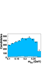
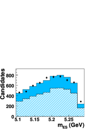
Refer to caption
Refer to caption
Refer to caption
Refer to caption
Refer to caption
Refer to caption
Figure 12: (color online) Comparison of off-resonance background to B0π+νsuperscript𝐵0superscript𝜋superscript𝜈B^{0}\rightarrow\pi^{-}\ell^{+}\nu samples for data and MC distributions. Top row: mESsubscript𝑚ESm_{\rm ES}, center row: ΔEΔ𝐸\Delta E, and bottom row: q2superscript𝑞2q^{2}, separately for the electron (left column) and muon (right column) samples. The shaded histograms indicate the true leptons, the hatched histograms indicate the fake leptons. The distributions are obtained from the full event selection, except for the qq¯𝑞¯𝑞q\bar{q} neural-network discrimination. Linear corrections have been applied to the simulation.
Refer to caption
Refer to caption
Refer to caption
Refer to caption
Refer to caption
Refer to caption
Figure 13: (color online) Comparison of off-resonance background to B0ρ+νsuperscript𝐵0superscript𝜌superscript𝜈B^{0}\rightarrow\rho^{-}\ell^{+}\nu samples for data and MC distributions. Top row: mESsubscript𝑚ESm_{\rm ES}, center row: ΔEΔ𝐸\Delta E, and bottom row: q2superscript𝑞2q^{2}, separately for the electron (left column) and muon (right column) samples. The shaded histograms indicate the true leptons, the hatched histograms indicate the fake leptons. The distributions are obtained from the full event selection, except for the qq¯𝑞¯𝑞q\bar{q} neural-network discrimination. Linear corrections have been applied to the simulation.

V.2 𝑩𝑿𝒄𝝂bold-→𝑩subscript𝑿𝒄bold-ℓ𝝂B\rightarrow X_{c}\ell\nu Enhanced Sample

The overall dominant background source in this analysis is BXcν𝐵subscript𝑋𝑐𝜈B\rightarrow X_{c}\ell\nu decays. Therefore it is important to verify that these decays are correctly simulated. This has been done in two ways, a) by relaxing the BXcν𝐵subscript𝑋𝑐𝜈B\rightarrow X_{c}\ell\nu suppression to obtain a charm-enhanced sample, and b) by reconstructing a specific decay mode, such as B0D+νsuperscript𝐵0superscript𝐷absentsuperscript𝜈B^{0}\rightarrow D^{*-}\ell^{+}\nu, in the same way we reconstruct the signal decays, and comparing the kinematic distributions with MC simulations (see Section V.3).

We select a charm-enhanced sample by inverting the cut on the BXcν𝐵subscript𝑋𝑐𝜈B\rightarrow X_{c}\ell\nu neural-network discriminator. Figures 14 and 15 show the ΔEΔ𝐸\Delta E and mESsubscript𝑚ESm_{\rm ES} distributions in the signal region and the side bands, as well as the q2superscript𝑞2q^{2} distribution in the signal region. All distributions show good agreement in shape; the absolute yields differ at a level that is expected, considering that the MC distributions have not been adjusted.
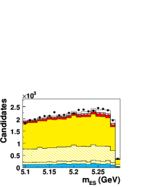
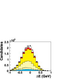
Refer to caption
Refer to caption
Refer to caption
Refer to caption
Refer to caption
Refer to caption
Refer to caption
Refer to caption
Refer to caption
Refer to caption
Figure 14: (color online) Comparison of data with MC distributions for the charm-enhanced selection for the B0π+νsuperscript𝐵0superscript𝜋superscript𝜈B^{0}\rightarrow\pi^{-}\ell^{+}\nu sample. Top row: mESsubscript𝑚ESm_{\rm ES} and ΔEΔ𝐸\Delta E for the signal bands, center row: mESsubscript𝑚ESm_{\rm ES} and ΔEΔ𝐸\Delta E for the side bands, and bottom row: qcorr2subscriptsuperscript𝑞2corrq^{2}_{\rm corr} for the whole fit region. The bin-by-bin ratio of data over the sum of all MC contributions is given in the plots below each histogram.
Refer to caption
Refer to caption
Refer to caption
Refer to caption
Refer to caption
Refer to caption
Refer to caption
Refer to caption
Refer to caption
Refer to caption
Figure 15: (color online) Comparison of data with MC distributions for the charm-enhanced selection for the B0ρ+νsuperscript𝐵0superscript𝜌superscript𝜈B^{0}\rightarrow\rho^{-}\ell^{+}\nu sample. Top row: mESsubscript𝑚ESm_{\rm ES} and ΔEΔ𝐸\Delta E for the signal bands, center row: mESsubscript𝑚ESm_{\rm ES} and ΔEΔ𝐸\Delta E for the side bands, and bottom row: qcorr2subscriptsuperscript𝑞2corrq^{2}_{\rm corr} for the whole fit region. The bin-by-bin ratios of data over the sum of all MC contributions is given in the plots below each histogram.

V.3 𝑩𝟎𝑫+𝝂bold-→superscript𝑩0superscript𝑫absentsuperscriptbold-ℓ𝝂B^{0}\rightarrow D^{*-}\ell^{+}\nu Control Sample

To study the Monte Carlo simulation of the neutrino reconstruction employed in this analysis, we use a control sample of exclusively reconstructed B0D+νsuperscript𝐵0superscript𝐷absentsuperscript𝜈B^{0}\rightarrow D^{*-}\ell^{+}\nu decays with DD¯πs0superscript𝐷absent¯𝐷superscriptsuperscriptsubscript𝜋𝑠0D^{*-}\rightarrow\kern 1.99997pt\overline{\kern-1.99997ptD}{}^{0}\pi_{s}^{-} and D¯0K+π\kern 1.99997pt\overline{\kern-1.99997ptD}{}^{0}\rightarrow K^{+}\pi^{-}. Since the B0D+νsuperscript𝐵0superscript𝐷absentsuperscript𝜈B^{0}\rightarrow D^{*-}\ell^{+}\nu decay rate exceeds the rate for B+ρ0+νsuperscript𝐵superscript𝜌0superscript𝜈B^{+}\rightarrow\rho^{0}\ell^{+}\nu by a factor of about 30 (including the D¯0\kern 1.99997pt\overline{\kern-1.99997ptD}{}^{0} branching fraction), this control sample represents a high-statistics and high-purity sample of exclusive semileptonic decays. Except for the low-momentum pion (πssuperscriptsubscript𝜋𝑠\pi_{s}^{-}), this final state has the same number of tracks, and very similar kinematics, as the B+ρ0+νsuperscript𝐵superscript𝜌0superscript𝜈B^{+}\rightarrow\rho^{0}\ell^{+}\nu signal decay. Furthermore, since about 50%percent5050\% of the BXcν𝐵subscript𝑋𝑐𝜈B\rightarrow X_{c}\ell\nu background in the Bπν𝐵𝜋𝜈B\rightarrow\pi\ell\nu and Bρν𝐵𝜌𝜈B\rightarrow\rho\ell\nu samples comes from B0D+νsuperscript𝐵0superscript𝐷absentsuperscript𝜈B^{0}\rightarrow D^{*-}\ell^{+}\nu decays, this B0D+νsuperscript𝐵0superscript𝐷absentsuperscript𝜈B^{0}\rightarrow D^{*-}\ell^{+}\nu sample can provide important tests of the shapes of the distributions that are used to discriminate the BXcν𝐵subscript𝑋𝑐𝜈B\rightarrow X_{c}\ell\nu background from signal.

Moreover, the distributions of the primary background suppression variables, in particular R2𝑅2R2, L2𝐿2L2, cosθBYsubscript𝜃BY\cos\theta_{\rm BY}, θmisssubscript𝜃miss\theta_{\rm miss}, and mmiss2/(2Emiss)superscriptsubscript𝑚miss22subscript𝐸missm_{\rm miss}^{2}/(2E_{\rm miss}), are relatively insensitive to the specific semileptonic decay mode. Likewise, the resolutions for the fit variables ΔEΔ𝐸\Delta E, mESsubscript𝑚ESm_{\rm ES}, and q2superscript𝑞2q^{2} are dominated by the resolution of the reconstructed neutrino, and thus depend little on the decay mode under study.

The reconstruction of the Dsuperscript𝐷absentD^{*-} from its decay products is straightforward. Except for the selection of the Dsuperscript𝐷absentD^{*-}, we apply the same preselection as for the signal charmless decays. We require the K+πsuperscript𝐾superscript𝜋K^{+}\pi^{-} invariant mass to be within 17 MeVMeV\mathrm{\,Me\kern-1.00006ptV} of the nominal D¯0\kern 1.99997pt\overline{\kern-1.99997ptD}{}^{0} mass, and restrict the mass difference, ΔmD=mDπmDΔsubscript𝑚superscript𝐷subscript𝑚𝐷𝜋subscript𝑚𝐷\Delta m_{D^{*}}=m_{D\pi}-m_{D} to 0.1432<ΔmD<0.1478GeV0.1432Δsubscript𝑚superscript𝐷0.1478GeV0.1432<\Delta m_{D^{*}}<0.1478\mathrm{\,Ge\kern-1.00006ptV}. The number of events in this data control sample exceeds the MC prediction by 3.8±1.7%plus-or-minus3.8percent1.73.8\pm 1.7\%, a result consistent with the uncertainties in the efficiency for the very-low-momentum charged pion from the DD¯π0superscript𝐷absent¯𝐷superscriptsuperscript𝜋0D^{*-}\rightarrow\kern 1.99997pt\overline{\kern-1.99997ptD}{}^{0}\pi^{-} decay. We correct the MC yield and sequentially place requirements on the same seven variables we use in the neural networks to both the data and MC samples. We compare the step-by-step reduction in the number of events; the largest difference is 0.9±0.7%plus-or-minus0.9percent0.70.9\pm 0.7\%, for the cut on cosθWsubscript𝜃𝑊\cos\theta_{W\ell}. For all other critical requirements the agreement is better than 0.5% and one standard deviation. The remaining background is at the level of 10%.

We have compared the MC-generated distributions for the control sample with the selected B0D+νsuperscript𝐵0superscript𝐷absentsuperscript𝜈B^{0}\rightarrow D^{*-}\ell^{+}\nu data sample and find very good agreement for the basic event variables, i.e., the multiplicity of charged particles and photons, and the total charge per event, indicating that the efficiency losses are well reproduced by the simulation. The distributions of the topological event variables R2𝑅2R2 and L2𝐿2L2 match well. Figure  16 shows the distributions of the variables critical for the neutrino reconstruction, pmiss,mmiss2/(2Emiss)subscript𝑝misssuperscriptsubscript𝑚miss22subscript𝐸missp_{\rm miss},m_{\rm miss}^{2}/(2E_{\rm miss}), cosθBYsubscript𝜃BY\cos\theta_{\rm BY}, and θmisssubscript𝜃miss\theta_{\rm miss}; they are also well reproduced.

Refer to caption
Figure 16: (color online) Comparison of data and MC-simulated distributions for the B0D+ν,D0¯K+πformulae-sequencesuperscript𝐵0superscript𝐷absentsuperscript𝜈¯superscript𝐷0superscript𝐾superscript𝜋B^{0}\rightarrow D^{*-}\ell^{+}\nu,\bar{D^{0}}\rightarrow K^{+}\pi^{-} sample, after selection criteria have been applied on all variables except the one presented. a) cosθBYsubscript𝜃BY\cos\theta_{\rm BY}, b) pmisssubscript𝑝missp_{\rm miss}, c) θmisssubscript𝜃miss\theta_{\rm miss}, d) cosθWsubscript𝜃𝑊\cos\theta_{W\ell}, e) mmiss2/2Emisssuperscriptsubscript𝑚miss22subscript𝐸missm_{\rm miss}^{2}/2E_{\rm miss}, and f) the total charge per event Qtotsubscript𝑄totQ_{\rm tot}. The background to the sample is indicated as a shaded (yellow) histogram. The combinatorial signal contribution is indicated as dashed histogram.

Figure 17 shows distributions of ΔEΔ𝐸\Delta E and mESsubscript𝑚ESm_{\rm ES} for events in the signal region and in the side bands. Again, the agreement between data and the MC simulation is reasonable.

We have also compared the q2superscript𝑞2q^{2} distributions of the simulation and the data control sample and find good agreement for both the raw and the corrected spectra, as illustrated in Figure 18. After corrections, no events appear above the kinematic limit of 10.7GeV210.7superscriptGeV210.7\mathrm{\,Ge\kern-1.00006ptV}^{2}. The qcorr2subscriptsuperscript𝑞2corrq^{2}_{\rm corr} resolution function can be described by the sum of two Gaussian resolution functions, with widths of 0.27GeV20.27superscriptGeV20.27\mathrm{\,Ge\kern-1.00006ptV}^{2} and 0.67GeV20.67superscriptGeV20.67\mathrm{\,Ge\kern-1.00006ptV}^{2}, close to the values obtained for events in the fit region for the signal Bπν𝐵𝜋𝜈B\rightarrow\pi\ell\nu and Bρν𝐵𝜌𝜈B\rightarrow\rho\ell\nu decays, respectively.

Refer to caption
Figure 17: (color online) Comparison of data and MC-simulated distributions for the B0D+ν,D0¯K+πformulae-sequencesuperscript𝐵0superscript𝐷absentsuperscript𝜈¯superscript𝐷0superscript𝐾superscript𝜋B^{0}\rightarrow D^{*-}\ell^{+}\nu,\bar{D^{0}}\rightarrow K^{+}\pi^{-} sample, after all selection cuts have been applied, a) ΔEΔ𝐸\Delta E for events in the mESsubscript𝑚ESm_{\rm ES} signal band, b) mESsubscript𝑚ESm_{\rm ES} for events in the ΔEΔ𝐸\Delta E signal band, c) ΔEΔ𝐸\Delta E for events in the mESsubscript𝑚ESm_{\rm ES} side band, and d) mESsubscript𝑚ESm_{\rm ES} for events in the ΔEΔ𝐸\Delta E side bands. The background to the sample is indicated as a shaded (yellow) histogram. The combinatorial signal contribution is indicated as dashed histogram.
Refer to caption
Figure 18: (color online) Comparison of the data and MC simulation of q2superscript𝑞2q^{2} distributions for the B0D+ν,D0¯K+πformulae-sequencesuperscript𝐵0superscript𝐷absentsuperscript𝜈¯superscript𝐷0superscript𝐾superscript𝜋B^{0}\rightarrow D^{*-}\ell^{+}\nu,\bar{D^{0}}\rightarrow K^{+}\pi^{-} sample after all selection criteria have been applied, a) the raw q2superscript𝑞2q^{2}, and b) the corrected q2superscript𝑞2q^{2}. The background to the sample is indicated as a shaded (yellow) histogram. The combinatorial signal contribution is indicated as dashed histogram.

VI Maximum-Likelihood Fit

VI.1 Overview

We determine the yields for the signal decay modes, B0π+νsuperscript𝐵0superscript𝜋superscript𝜈B^{0}\rightarrow\pi^{-}\ell^{+}\nu, B+π0+νsuperscript𝐵superscript𝜋0superscript𝜈B^{+}\rightarrow\pi^{0}\ell^{+}\nu, B0ρ+νsuperscript𝐵0superscript𝜌superscript𝜈B^{0}\rightarrow\rho^{-}\ell^{+}\nu, and B+ρ0+νsuperscript𝐵superscript𝜌0superscript𝜈B^{+}\rightarrow\rho^{0}\ell^{+}\nu, by performing a maximum-likelihood fit to the three-dimensional ΔEmESq2Δ𝐸subscript𝑚ESsuperscript𝑞2\Delta E-m_{\rm ES}-q^{2} distributions for the four selected data samples corresponding to the four exclusive decay modes. The fit technique employed in this analysis is an extended binned maximum-likelihood fit that accounts for the statistical fluctuations not only of the data samples but also of the MC samples by allowing the MC-simulated distributions to fluctuate in each bin according to the statistical uncertainty given by the number of events in the bin. This method was introduced by Barlow and Beeston BarlowFit .

The parameters of the fit are scale factors for the signal and background yields of the four selected event samples. We use the following nomenclature for the fit parameters: pjsourcesuperscriptsubscript𝑝𝑗𝑠𝑜𝑢𝑟𝑐𝑒p_{j}^{source}, where the superscript source𝑠𝑜𝑢𝑟𝑐𝑒source denotes the fit source (signal or background type) and the subscript j𝑗j labels the qcorr2subscriptsuperscript𝑞2corrq^{2}_{\rm corr} bin (if no subscript is given, the same fit parameter is used across all q2superscript𝑞2q^{2} bins). Predictions for the shape of the ΔEmESΔ𝐸subscript𝑚ES\Delta E-m_{\rm ES} distributions are taken from simulation of both signal and the various background sources, separately for each bin in q2superscript𝑞2q^{2}. The branching fractions for the four signal decays are obtained by multiplying the fitted values of the scale factors with the branching fractions that are implemented in the MC simulation.

The choice of a two-dimensional distribution in ΔEΔ𝐸\Delta E and mESsubscript𝑚ESm_{\rm ES}  is mandated because the two variables are correlated for both signal, in particular the combinatorial signal events, and for some of the background sources. Since it would be difficult to determine reliable analytic expressions for these two-dimensional distributions, a binned maximum-likelihood method is used, with the bin sizes chosen to obtain a good signal and background separation while retaining adequate statistics in all bins. The bin sizes are small in the region where most of the signal is located and larger in the side bands. There are 47 ΔEmESΔ𝐸subscript𝑚ES\Delta E-m_{\rm ES} bins for each bin in qcorr2subscriptsuperscript𝑞2corrq^{2}_{\rm corr}. Figure 19 shows the ΔEmESΔ𝐸subscript𝑚ES\Delta E-m_{\rm ES} distribution for signal events and the binning used in the fit. As mentioned in Section IV.2.2, for the two Bπν𝐵𝜋𝜈B\rightarrow\pi\ell\nu samples the q2superscript𝑞2q^{2} range 0<qcorr2<26.4GeV20subscriptsuperscript𝑞2corr26.4superscriptGeV20<q^{2}_{\rm corr}<26.4\mathrm{\,Ge\kern-1.00006ptV}^{2} is divided into six bins, and for the two Bρν𝐵𝜌𝜈B\rightarrow\rho\ell\nu samples the range 0<qcorr2<20.3GeV20subscriptsuperscript𝑞2corr20.3superscriptGeV20<q^{2}_{\rm corr}<20.3\mathrm{\,Ge\kern-1.00006ptV}^{2} is divided into three bins.

Refer to caption Refer to caption
Figure 19: Distribution of ΔEΔ𝐸\Delta E vs mESsubscript𝑚ESm_{\rm ES} for true B0π+νsuperscript𝐵0superscript𝜋superscript𝜈B^{0}\rightarrow\pi^{-}\ell^{+}\nu signal events (left) and definition of bins in the ΔEmESΔ𝐸subscript𝑚ES\Delta E-m_{\rm ES} plane used in the fit for all samples (right).

VI.2 Fit Method

Since the MC samples available to create the probability density functions (PDFs) for the individual sources that are input to the fits are rather limited in size, it is necessary to take into account the statistical uncertainties, given by the number of events generated for each bin. For this reason we have adopted a generalized binned maximum-likelihood fit method. The MC samples that are used to define the PDFs are to a good approximation statistically independent of those used to train the neural networks for background suppression, since for the latter relatively small subsamples of the full MC samples have been used.

As mentioned above, the data are divided into n𝑛n bins in a three-dimensional array in ΔEmESqcorr2Δ𝐸subscript𝑚ESsubscriptsuperscript𝑞2corr\Delta E-m_{\rm ES}-q^{2}_{\rm corr}.

If disubscript𝑑𝑖d_{i} is the number of selected events in bin i𝑖i for a given single data sample corresponding to candidates for a specific decay mode, and ajisubscript𝑎𝑗𝑖a_{ji} is the number of MC events from source j𝑗j in this bin, then

ND=i=1ndi,Nj=i=1naji,formulae-sequencesubscript𝑁𝐷superscriptsubscript𝑖1𝑛subscript𝑑𝑖subscript𝑁𝑗superscriptsubscript𝑖1𝑛subscript𝑎𝑗𝑖N_{D}=\sum_{i=1}^{n}d_{i},\hskip 28.45274ptN_{j}=\sum_{i=1}^{n}a_{ji}, (24)

where NDsubscript𝑁𝐷N_{D} is the total number of events in the data sample, and Njsubscript𝑁𝑗N_{j} is the total number in the MC sample for source j𝑗j. We assume that there are m𝑚m different MC-generated source distributions that add up to describe the data. The predicted number of events in each bin fi(Pj)subscript𝑓𝑖subscript𝑃𝑗f_{i}(P_{j}) can be written in terms of the strength of the individual contributions Pjsubscript𝑃𝑗P_{j} (j=1,..,mj=1,..,m) as

fi=NDj=1mPjwjiaji/Nj=j=1mpjwjiaji,subscript𝑓𝑖subscript𝑁𝐷superscriptsubscript𝑗1𝑚subscript𝑃𝑗subscript𝑤𝑗𝑖subscript𝑎𝑗𝑖subscript𝑁𝑗superscriptsubscript𝑗1𝑚subscript𝑝𝑗subscript𝑤𝑗𝑖subscript𝑎𝑗𝑖f_{i}=N_{D}\sum_{j=1}^{m}P_{j}w_{ji}a_{ji}/N_{j}=\sum_{j=1}^{m}p_{j}w_{ji}a_{ji}, (25)

with pj=NDPj/Njsubscript𝑝𝑗subscript𝑁𝐷subscript𝑃𝑗subscript𝑁𝑗p_{j}=N_{D}P_{j}/N_{j}. In each bin, the weights wjisubscript𝑤𝑗𝑖w_{ji} account for the relative normalization of the samples and various other corrections.

Since the MC samples are limited in size, the generated numbers of events ajisubscript𝑎𝑗𝑖a_{ji} have statistical fluctuations relative to the value Ajisubscript𝐴𝑗𝑖A_{ji} expected for infinite statistics, and thus the more correct prediction for each bin is

fi=j=1mpjwjiAji.subscript𝑓𝑖superscriptsubscript𝑗1𝑚subscript𝑝𝑗subscript𝑤𝑗𝑖subscript𝐴𝑗𝑖f_{i}=\sum_{j=1}^{m}p_{j}w_{ji}A_{ji}. (26)

If we assume Poisson statistics for both the data and MC samples, the total likelihood function {\cal L} is the combined probability for the observed disubscript𝑑𝑖d_{i} and ajisubscript𝑎𝑗𝑖a_{ji} BarlowFit ,

ln=i=1n(dilnfifi)+i=1nj=1m(ajilnAjiAji).superscriptsubscript𝑖1𝑛subscript𝑑𝑖subscript𝑓𝑖subscript𝑓𝑖superscriptsubscript𝑖1𝑛superscriptsubscript𝑗1𝑚subscript𝑎𝑗𝑖subscript𝐴𝑗𝑖subscript𝐴𝑗𝑖\ln{\cal L}=\sum_{i=1}^{n}(d_{i}\ln f_{i}-f_{i})+\sum_{i=1}^{n}\sum_{j=1}^{m}(a_{ji}\ln A_{ji}-A_{ji}). (27)

The first sum has the usual form associated with the uncertainty of the data and the second term refers to the MC statistics and is not dependent on data. There are (n+1)×m𝑛1𝑚(n+1)\times m unknown parameters that need to be determined: the m𝑚m relative normalization factors pjsubscript𝑝𝑗p_{j}, which are of interest to the signal extraction, and n×m𝑛𝑚n\times m values Ajisubscript𝐴𝑗𝑖A_{ji}.

The problem can be significantly simplified. The n×m𝑛𝑚n\times m quantities Ajisubscript𝐴𝑗𝑖A_{ji} can be determined by solving n𝑛n simultaneous equations for Ajisubscript𝐴𝑗𝑖A_{ji} of the form

fi=j=1mpjwjiAji=j=1mpjwjiaji1+pjwjiti,subscript𝑓𝑖superscriptsubscript𝑗1𝑚subscript𝑝𝑗subscript𝑤𝑗𝑖subscript𝐴𝑗𝑖superscriptsubscript𝑗1𝑚subscript𝑝𝑗subscript𝑤𝑗𝑖subscript𝑎𝑗𝑖1subscript𝑝𝑗subscript𝑤𝑗𝑖subscript𝑡𝑖f_{i}=\sum_{j=1}^{m}p_{j}w_{ji}A_{ji}=\sum_{j=1}^{m}\frac{p_{j}w_{ji}a_{ji}}{1+p_{j}w_{ji}t_{i}}, (28)

with Aji=aji/(1+pjwjiti)subscript𝐴𝑗𝑖subscript𝑎𝑗𝑖1subscript𝑝𝑗subscript𝑤𝑗𝑖subscript𝑡𝑖A_{ji}=a_{ji}/(1+p_{j}w_{ji}t_{i}) and ti=1di/fisubscript𝑡𝑖1subscript𝑑𝑖subscript𝑓𝑖t_{i}=1-d_{i}/f_{i} (for di=0subscript𝑑𝑖0d_{i}=0 we define ti=1subscript𝑡𝑖1t_{i}=1). At every step in the minimization of 22-2ln{\cal L} these n𝑛n independent equations need to be solved. This procedure results not only in the determination of the parameters pjsubscript𝑝𝑗p_{j}, but also in improved estimates for the various contributions Ajisubscript𝐴𝑗𝑖A_{ji} in each bin.

For fits to the individual data samples corresponding to the four signal decay modes, there is a specific likelihood function (Eq. 27). To perform a simultaneous fit to all four data samples the log-likelihood function is the sum of the individual ones. Some of the parameters pjsubscript𝑝𝑗p_{j} may be shared among the four likelihood functions,

ln=h=14lnhsuperscriptsubscript14subscript\displaystyle\ln{\cal L}=\sum_{h=1}^{4}\ln{\cal L}_{h} =\displaystyle= h=14i=1n(dhilnfhifhi)superscriptsubscript14superscriptsubscript𝑖1𝑛subscript𝑑𝑖subscript𝑓𝑖subscript𝑓𝑖\displaystyle\sum_{h=1}^{4}\sum_{i=1}^{n}{(d_{hi}\ln{f_{hi}}-f_{hi})}
+\displaystyle+ h=14i=1nj=1m(ahjilnAhjiAhji).superscriptsubscript14superscriptsubscript𝑖1𝑛superscriptsubscript𝑗1𝑚subscript𝑎𝑗𝑖subscript𝐴𝑗𝑖subscript𝐴𝑗𝑖\displaystyle\sum_{h=1}^{4}{\sum_{i=1}^{n}\sum_{j=1}^{m}{(a_{hji}\ln{A_{hji}}-A_{hji})}}.

VI.3 Fit Parameters and Inputs

The fits can be performed separately for each of the four data samples or combined for all four data samples, and where possible, with common fit parameters. The nominal fit in this analysis is a simultaneous fit of all four data samples: B0π+νsuperscript𝐵0superscript𝜋superscript𝜈B^{0}\rightarrow\pi^{-}\ell^{+}\nu, B+π0+νsuperscript𝐵superscript𝜋0superscript𝜈B^{+}\rightarrow\pi^{0}\ell^{+}\nu, B0ρ+νsuperscript𝐵0superscript𝜌superscript𝜈B^{0}\rightarrow\rho^{-}\ell^{+}\nu, and B+ρ0+νsuperscript𝐵superscript𝜌0superscript𝜈B^{+}\rightarrow\rho^{0}\ell^{+}\nu. A signal decay in one data sample may contribute to the background in another sample, and therefore these sources share a common fit parameter. For example, the scale factor for the B0ρ+νsuperscript𝐵0superscript𝜌superscript𝜈B^{0}\rightarrow\rho^{-}\ell^{+}\nu signal in the B0ρ+νsuperscript𝐵0superscript𝜌superscript𝜈B^{0}\rightarrow\rho^{-}\ell^{+}\nu sample is also applied in the B0π+νsuperscript𝐵0superscript𝜋superscript𝜈B^{0}\rightarrow\pi^{-}\ell^{+}\nu sample, where it represents cross-feed background.

We impose isospin invariance for the signal decay modes,

Γ(B0π+ν)Γsuperscript𝐵0superscript𝜋superscript𝜈\displaystyle\Gamma(B^{0}\rightarrow\pi^{-}\ell^{+}\nu) =\displaystyle= 2Γ(B+π0+ν),2Γsuperscript𝐵superscript𝜋0superscript𝜈\displaystyle 2\Gamma(B^{+}\rightarrow\pi^{0}\ell^{+}\nu),
Γ(B0ρ+ν)Γsuperscript𝐵0superscript𝜌superscript𝜈\displaystyle\Gamma(B^{0}\rightarrow\rho^{-}\ell^{+}\nu) =\displaystyle= 2Γ(B+ρ0+ν).2Γsuperscript𝐵superscript𝜌0superscript𝜈\displaystyle 2\Gamma(B^{+}\rightarrow\rho^{0}\ell^{+}\nu)\ . (30)

The yields of the true and combinatorial signal decays as well as isospin-conjugate decays are related to the same branching fraction and therefore share the same fit parameter. The BXuν𝐵subscript𝑋𝑢𝜈B\rightarrow X_{u}\ell\nu background, which contains exclusive and non-resonant decays, is scaled by two parameters, one for low and intermediate q2superscript𝑞2q^{2} (q2<20GeV2superscript𝑞220superscriptGeV2q^{2}<20\mathrm{\,Ge\kern-1.00006ptV}^{2}) and one for high q2superscript𝑞2q^{2} (q2>20GeV2superscript𝑞220superscriptGeV2q^{2}>20\mathrm{\,Ge\kern-1.00006ptV}^{2}), for the fits to the Bπν𝐵𝜋𝜈B\rightarrow\pi\ell\nu samples. Because of the large correlation between BXuν𝐵subscript𝑋𝑢𝜈B\rightarrow X_{u}\ell\nu background and Bρν𝐵𝜌𝜈B\rightarrow\rho\ell\nu signal (>90%absentpercent90>90\% for both Bρν𝐵𝜌𝜈B\rightarrow\rho\ell\nu modes), we rely on MC simulation for the BXuν𝐵subscript𝑋𝑢𝜈B\rightarrow X_{u}\ell\nu background and keep it fixed in the fits to the Bρν𝐵𝜌𝜈B\rightarrow\rho\ell\nu samples. The BB¯𝐵¯𝐵B\kern 1.79993pt\overline{\kern-1.79993ptB}{} background is split into two sources. Among the BXcν𝐵subscript𝑋𝑐𝜈B\rightarrow X_{c}\ell\nu decays, we treat the dominant decay mode, BDν𝐵superscript𝐷𝜈B\rightarrow D^{*}\ell\nu, as a separate source and combine the other semileptonic decays (BDν𝐵𝐷𝜈B\rightarrow D\ell\nu, BD()(nπ)ν𝐵superscript𝐷𝑛𝜋𝜈B\rightarrow D^{(*)}(n\pi)\ell\nu) and the remaining (or “other”) BB¯𝐵¯𝐵B\kern 1.79993pt\overline{\kern-1.79993ptB}{} background (secondary leptons and fake leptons) into a single source. The continuum qq¯𝑞¯𝑞q\overline{q} background sources containing true and fake leptons are combined into one fit source and scaled by a single fit parameter.

The complete list of fit sources and corresponding fit parameters is given in Table 6. The πρ𝜋𝜌\pi\leftrightarrow\rho cross feed is a free fit parameter in the four-mode fit; for one-mode fits, it is fixed to the value obtained from the four-mode fit. In the four-mode fit, all background sources that are not fixed are fit separately for each signal mode, since the different hadrons of the signal decays lead to different combinatorial backgrounds.

Table 6: List of fit parameters representing scale factors for the different signal samples and background sources. Parameters with index j𝑗j are free parameters in the fit, one for each q2superscript𝑞2q^{2} bin j𝑗j. The πρ𝜋𝜌\pi\leftrightarrow\rho crossfeed parameter is free only in the four-mode fit; for one-mode fits, it is fixed to the values obtained from the four-mode fit. There are independent scale factors for qq¯𝑞¯𝑞q\overline{q} background, BDν𝐵superscript𝐷𝜈B\rightarrow D^{*}\ell\nu decays and for all other background sources from BB¯𝐵¯𝐵B\kern 1.79993pt\overline{\kern-1.79993ptB}{} events for all four signal modes (subscripts π±,π0,ρ±,ρ0superscript𝜋plus-or-minussuperscript𝜋0superscript𝜌plus-or-minussuperscript𝜌0\pi^{\pm},\pi^{0},\rho^{\pm},\rho^{0}). For the Bπν𝐵𝜋𝜈B\rightarrow\pi\ell\nu decays, the BXuν𝐵subscript𝑋𝑢𝜈B\rightarrow X_{u}\ell\nu background is fit in two q2superscript𝑞2q^{2} intervals (index k=1,2𝑘12k=1,2); for the Bρν𝐵𝜌𝜈B\rightarrow\rho\ell\nu decays it is fixed.
Source / sample Bπν𝐵𝜋𝜈B\rightarrow\pi\ell\nu Bρν𝐵𝜌𝜈B\rightarrow\rho\ell\nu
Signal pjπνsuperscriptsubscript𝑝𝑗𝜋𝜈p_{j}^{\pi\ell\nu} pjρνsuperscriptsubscript𝑝𝑗𝜌𝜈p_{j}^{\rho\ell\nu}
Combinatorial signal pjπνsuperscriptsubscript𝑝𝑗𝜋𝜈p_{j}^{\pi\ell\nu} pjρνsuperscriptsubscript𝑝𝑗𝜌𝜈p_{j}^{\rho\ell\nu}
Isospin-conjugate signal pjπνsuperscriptsubscript𝑝𝑗𝜋𝜈p_{j}^{\pi\ell\nu} pjρνsuperscriptsubscript𝑝𝑗𝜌𝜈p_{j}^{\rho\ell\nu}
Cross feed πρ𝜋𝜌\pi\leftrightarrow\rho pjρνsuperscriptsubscript𝑝𝑗𝜌𝜈p_{j}^{\rho\ell\nu} pjπνsuperscriptsubscript𝑝𝑗𝜋𝜈p_{j}^{\pi\ell\nu}
BXuν𝐵subscript𝑋𝑢𝜈B\rightarrow X_{u}\ell\nu background pπ±,kuνsubscriptsuperscript𝑝𝑢𝜈superscript𝜋plus-or-minus𝑘p^{u\ell\nu}_{\pi^{\pm},k}, pπ0,kuνsubscriptsuperscript𝑝𝑢𝜈superscript𝜋0𝑘p^{u\ell\nu}_{\pi^{0},k} fixed
BDν𝐵superscript𝐷𝜈B\rightarrow D^{*}\ell\nu background pπ±Dνsuperscriptsubscript𝑝superscript𝜋plus-or-minussuperscript𝐷𝜈p_{\pi^{\pm}}^{D^{*}\ell\nu}, pπ0Dνsuperscriptsubscript𝑝superscript𝜋0superscript𝐷𝜈p_{\pi^{0}}^{D^{*}\ell\nu} pρ±Dνsuperscriptsubscript𝑝superscript𝜌plus-or-minussuperscript𝐷𝜈p_{\rho^{\pm}}^{D^{*}\ell\nu}, pρ0Dνsuperscriptsubscript𝑝superscript𝜌0superscript𝐷𝜈p_{\rho^{0}}^{D^{*}\ell\nu}
Other BB¯𝐵¯𝐵B\kern 1.79993pt\overline{\kern-1.79993ptB}{} background pπ±otherBB¯superscriptsubscript𝑝superscript𝜋plus-or-minus𝑜𝑡𝑒𝑟𝐵¯𝐵p_{\pi^{\pm}}^{otherB\kern 1.25995pt\overline{\kern-1.25995ptB}{}}, pπ0otherBB¯superscriptsubscript𝑝superscript𝜋0𝑜𝑡𝑒𝑟𝐵¯𝐵p_{\pi^{0}}^{otherB\kern 1.25995pt\overline{\kern-1.25995ptB}{}} pρ±otherBB¯superscriptsubscript𝑝superscript𝜌plus-or-minus𝑜𝑡𝑒𝑟𝐵¯𝐵p_{\rho^{\pm}}^{otherB\kern 1.25995pt\overline{\kern-1.25995ptB}{}}, pρ0otherBB¯superscriptsubscript𝑝superscript𝜌0𝑜𝑡𝑒𝑟𝐵¯𝐵p_{\rho^{0}}^{otherB\kern 1.25995pt\overline{\kern-1.25995ptB}{}}
qq¯𝑞¯𝑞q\overline{q} background pπ±qq¯superscriptsubscript𝑝superscript𝜋plus-or-minus𝑞¯𝑞p_{\pi^{\pm}}^{q\overline{q}}, pπ0qq¯superscriptsubscript𝑝superscript𝜋0𝑞¯𝑞p_{\pi^{0}}^{q\overline{q}} pρ±qq¯superscriptsubscript𝑝superscript𝜌plus-or-minus𝑞¯𝑞p_{\rho^{\pm}}^{q\overline{q}}, pρ0qq¯superscriptsubscript𝑝superscript𝜌0𝑞¯𝑞p_{\rho^{0}}^{q\overline{q}}

VI.4 Fit Results

The fits are performed both separately and simultaneously for the four signal decay modes, B0π+νsuperscript𝐵0superscript𝜋superscript𝜈B^{0}\rightarrow\pi^{-}\ell^{+}\nu, B+π0+νsuperscript𝐵superscript𝜋0superscript𝜈B^{+}\rightarrow\pi^{0}\ell^{+}\nu, B0ρ+νsuperscript𝐵0superscript𝜌superscript𝜈B^{0}\rightarrow\rho^{-}\ell^{+}\nu, and B+ρ0+νsuperscript𝐵superscript𝜌0superscript𝜈B^{+}\rightarrow\rho^{0}\ell^{+}\nu. Figures 2023 show projections of the fitted ΔEmESΔ𝐸subscript𝑚ES\Delta E-m_{\rm ES} distributions in the signal bands for these decays, separately for each bin in qcorr2subscriptsuperscript𝑞2corrq^{2}_{\rm corr}. As a measure of the goodness-of-fit we use χ2superscript𝜒2\chi^{2} per degree of freedom; all fits have values in the range 1.051.111.051.111.05-1.11 (for details see Table 7).

The scale factors for the signal contributions, which are determined by the fits, can be translated to numbers of background-subtracted signal events for the four signal decays. These signal yields are listed in Table 7 with errors that are a combination of the statistical uncertainties of the data and MC samples and the uncertainties of the fitted yields of the various backgrounds. For each signal decay mode, the table specifies the number of true and combinatorial signal decays. Their relative fraction is taken from simulation. This fraction is larger for decays with a π0superscript𝜋0\pi^{0} in the final state. For all signal modes, the fraction of combinatorial signal events is small at low q2superscript𝑞2q^{2}, increases with q2superscript𝑞2q^{2}, and at the highest q2superscript𝑞2q^{2} it is similar to or exceeds the one of true signal decays. This leads to larger errors in the measurement of q2superscript𝑞2q^{2}, mESsubscript𝑚ESm_{\rm ES} and ΔEΔ𝐸\Delta E.

In Table 17 in Appendix XI.2 the correlation matrix of the four-mode fit is presented. We observe correlations of about 4060%40percent6040-60\% between the qq¯𝑞¯𝑞q\overline{q} and the other BB¯𝐵¯𝐵B\kern 1.79993pt\overline{\kern-1.79993ptB}{} backgrounds and between the BDν𝐵superscript𝐷𝜈B\rightarrow D^{*}\ell\nu and the other BB¯𝐵¯𝐵B\kern 1.79993pt\overline{\kern-1.79993ptB}{} backgrounds for all signal modes. For Bπν𝐵𝜋𝜈B\rightarrow\pi\ell\nu, the correlation between the BXuν𝐵subscript𝑋𝑢𝜈B\rightarrow X_{u}\ell\nu background and the signal at high q2superscript𝑞2q^{2} is also sizable (60%similar-to-or-equalsabsentpercent60\simeq 60\%). For Bρν𝐵𝜌𝜈B\rightarrow\rho\ell\nu, this correlation is larger than 90%percent9090\%, which is why we choose to fix the BXuν𝐵subscript𝑋𝑢𝜈B\rightarrow X_{u}\ell\nu background normalization for these two samples. As a test, we let the BXuν𝐵subscript𝑋𝑢𝜈B\rightarrow X_{u}\ell\nu background normalization in the Bρν𝐵𝜌𝜈B\rightarrow\rho\ell\nu modes vary as free parameter in the four-mode fit. This results in a BXuν𝐵subscript𝑋𝑢𝜈B\rightarrow X_{u}\ell\nu contribution that is lower by a factor of 0.85±0.15plus-or-minus0.850.150.85\pm 0.15 for B0ρ+νsuperscript𝐵0superscript𝜌superscript𝜈B^{0}\rightarrow\rho^{-}\ell^{+}\nu  and 0.90±0.14plus-or-minus0.900.140.90\pm 0.14 for B+ρ0+νsuperscript𝐵superscript𝜌0superscript𝜈B^{+}\rightarrow\rho^{0}\ell^{+}\nu and an increase of the Bρν𝐵𝜌𝜈B\rightarrow\rho\ell\nu signal yields by 10%percent1010\% in the first two q2superscript𝑞2q^{2} bins and by 15%percent1515\% in the last q2superscript𝑞2q^{2} bin. These changes are covered by the systematic uncertainties due to the BXuν𝐵subscript𝑋𝑢𝜈B\rightarrow X_{u}\ell\nu background stated in Section VII.

To cross-check the results of the nominal four-mode fit, we also perform fits for each signal mode separately. The contributions from the other signal decay modes are fixed to the result obtained from the four-mode fit. Since the shape of the πρ𝜋𝜌\pi\leftrightarrow\rho cross-feed contribution is very similar to the other BXuν𝐵subscript𝑋𝑢𝜈B\rightarrow X_{u}\ell\nu background, we fix its normalization to the one obtained from the four-mode fit. A comparison of the results of the one-mode fits with the combined four-mode fit shows agreement within the fit errors of the B0π+νsuperscript𝐵0superscript𝜋superscript𝜈B^{0}\rightarrow\pi^{-}\ell^{+}\nu and B+π0+νsuperscript𝐵superscript𝜋0superscript𝜈B^{+}\rightarrow\pi^{0}\ell^{+}\nu modes and the B0ρ+νsuperscript𝐵0superscript𝜌superscript𝜈B^{0}\rightarrow\rho^{-}\ell^{+}\nu and B+ρ0+νsuperscript𝐵superscript𝜌0superscript𝜈B^{+}\rightarrow\rho^{0}\ell^{+}\nu modes in all q2superscript𝑞2q^{2} bins.

The partial branching fractions for the different qcorr2subscriptsuperscript𝑞2corrq^{2}_{\rm corr} bins are derived as the products of the fitted signal scale factors and the signal decay branching fractions used in the simulation. The total branching fraction integrated over the entire q2superscript𝑞2q^{2} range and its error are calculated as the sum of all partial branching fractions, taking into account the correlations of the fitted yields in different q2superscript𝑞2q^{2} bins. The branching fraction for B0superscript𝐵0B^{0} decays, signal0subscriptsuperscript0signal{\cal B}^{0}_{\rm signal}, is related to the fitted signal yields, Nsignal0subscriptsuperscript𝑁0signalN^{0}_{\rm signal}, in the following way,

signal0=Nsignal04×ϵsignal0f00NBB¯,subscriptsuperscript0signalsubscriptsuperscript𝑁0signal4subscriptsuperscriptitalic-ϵ0signalsubscript𝑓00subscript𝑁𝐵¯𝐵{\cal B}^{0}_{\rm signal}=\frac{N^{0}_{\rm signal}}{4\times\epsilon^{0}_{\rm signal}f_{00}N_{B\kern 1.25995pt\overline{\kern-1.25995ptB}{}}}\ , (31)

where f00=0.484±0.006subscript𝑓00plus-or-minus0.4840.006f_{00}=0.484\pm 0.006 HFAG2009 denotes the fraction of B0B0¯superscript𝐵0¯superscript𝐵0B^{0}\bar{B^{0}} events produced in Υ(4S)Υ4𝑆\mathchar 28935\relax{(4S)} decays and ϵsignal0subscriptsuperscriptitalic-ϵ0signal\epsilon^{0}_{\rm signal} is the total signal efficiency (averaged over the electron and muon samples) as predicted by the MC simulation. The factor of four accounts for the fact that each event contains two B𝐵B mesons, and that the branching fraction is quoted for a single charged lepton, not for the sum of the decays to electrons or muons. The branching fraction results are presented in Section VIII.
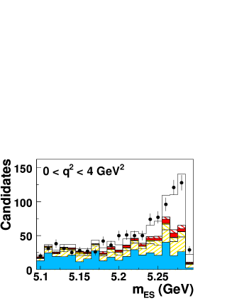
Refer to captionRefer to caption Refer to captionRefer to caption Refer to captionRefer to caption
Figure 20: (color online) mESsubscript𝑚ESm_{\rm ES} and ΔEΔ𝐸\Delta E distributions in each q2superscript𝑞2q^{2} bin for B0π+νsuperscript𝐵0superscript𝜋superscript𝜈B^{0}\rightarrow\pi^{-}\ell^{+}\nu after the fit. The distributions are shown in the ΔEΔ𝐸\Delta E and mESsubscript𝑚ESm_{\rm ES} signal bands, respectively. Legend: see Figure 5.
Refer to captionRefer to caption Refer to captionRefer to caption Refer to captionRefer to caption
Figure 21: (color online) mESsubscript𝑚ESm_{\rm ES} and ΔEΔ𝐸\Delta E distributions in each q2superscript𝑞2q^{2} bin for B+π0+νsuperscript𝐵superscript𝜋0superscript𝜈B^{+}\rightarrow\pi^{0}\ell^{+}\nu after the fit. The distributions are shown in the ΔEΔ𝐸\Delta E and mESsubscript𝑚ESm_{\rm ES} signal bands, respectively. Legend: see Figure 5.
Refer to captionRefer to caption Refer to captionRefer to caption Refer to captionRefer to caption
Figure 22: (color online) mESsubscript𝑚ESm_{\rm ES} and ΔEΔ𝐸\Delta E distributions in each q2superscript𝑞2q^{2} bin for B0ρ+νsuperscript𝐵0superscript𝜌superscript𝜈B^{0}\rightarrow\rho^{-}\ell^{+}\nu after the fit. The distributions are shown in the ΔEΔ𝐸\Delta E and mESsubscript𝑚ESm_{\rm ES} signal bands, respectively. Legend: see Figure 5.
Refer to captionRefer to caption Refer to captionRefer to caption Refer to captionRefer to caption
Figure 23: (color online) mESsubscript𝑚ESm_{\rm ES} and ΔEΔ𝐸\Delta E distributions in each q2superscript𝑞2q^{2} bin for B+ρ0+νsuperscript𝐵superscript𝜌0superscript𝜈B^{+}\rightarrow\rho^{0}\ell^{+}\nu after the fit. The distributions are shown in the ΔEΔ𝐸\Delta E and mESsubscript𝑚ESm_{\rm ES} signal bands, respectively. Legend: see Figure 5.
Table 7: Results of fits performed separately for each of the four signal decay modes and simultaneously for all four decay modes in bins of q2superscript𝑞2q^{2}: χ2superscript𝜒2\chi^{2} per degree of freedom, signal yields for true signal decays, Nsigsuperscript𝑁sigN^{\rm sig}, and combinatorial signal, Ncombsuperscript𝑁combN^{\rm comb}. The stated errors are the fit errors.
q2superscript𝑞2q^{2} range (GeV2superscriptGeV2\mathrm{\,Ge\kern-1.00006ptV}^{2}) χ2/ndfsuperscript𝜒2𝑛𝑑𝑓\chi^{2}/ndf 0-4 4-8 8-12 12-16 16-20 >> 20 0<q2<26.40superscript𝑞226.40<q^{2}<26.4
Nπ±sigsubscriptsuperscript𝑁𝑠𝑖𝑔superscript𝜋plus-or-minusN^{sig}_{\pi^{\pm}} 259/268 701±64plus-or-minus70164701\pm 64 1950±104plus-or-minus19501041950\pm 104 1552±113plus-or-minus15521131552\pm 113 1184±104plus-or-minus11841041184\pm 104 732±80plus-or-minus73280732\pm 80 541±68plus-or-minus54168541\pm 68 6660±2 78plus-or-minus66602786660\pm 2\ 78
Nπ±combsubscriptsuperscript𝑁𝑐𝑜𝑚𝑏superscript𝜋plus-or-minusN^{comb}_{\pi^{\pm}} 1±0.1plus-or-minus10.11\pm 0.1 4±0.2plus-or-minus40.24\pm 0.2 9±1plus-or-minus919\pm 1 30±3plus-or-minus30330\pm 3 77±8plus-or-minus77877\pm 8 401±51plus-or-minus40151401\pm 51 521±22plus-or-minus52122521\pm 22
Nπ±=Nπ±sig+Nπ±combsubscript𝑁superscript𝜋plus-or-minussubscriptsuperscript𝑁𝑠𝑖𝑔superscript𝜋plus-or-minussubscriptsuperscript𝑁𝑐𝑜𝑚𝑏superscript𝜋plus-or-minusN_{\pi^{\pm}}=N^{sig}_{\pi^{\pm}}+N^{comb}_{\pi^{\pm}} 702±64plus-or-minus70264702\pm 64 1954±104plus-or-minus19541041954\pm 104 1561±113plus-or-minus15611131561\pm 113 1214±104plus-or-minus12141041214\pm 104 809±80plus-or-minus80980809\pm 80 942±85plus-or-minus94285942\pm 85 7181±279plus-or-minus71812797181\pm 279
Nπ0sigsubscriptsuperscript𝑁𝑠𝑖𝑔superscript𝜋0N^{sig}_{\pi^{0}} 237/268 315±42plus-or-minus31542315\pm 42 576±54plus-or-minus57654576\pm 54 904±107plus-or-minus904107904\pm 107 471±68plus-or-minus47168471\pm 68 414±83plus-or-minus41483414\pm 83 159±55plus-or-minus15955159\pm 55 2840±203plus-or-minus28402032840\pm 203
Nπ0combsubscriptsuperscript𝑁𝑐𝑜𝑚𝑏superscript𝜋0N^{comb}_{\pi^{0}} 5±0.7plus-or-minus50.75\pm 0.7 13±1plus-or-minus13113\pm 1 36±4plus-or-minus36436\pm 4 36±5plus-or-minus36536\pm 5 119±24plus-or-minus11924119\pm 24 397±137plus-or-minus397137397\pm 137 606±43plus-or-minus60643606\pm 43
Nπ0=Nπ0sig+Nπ0combsubscript𝑁superscript𝜋0subscriptsuperscript𝑁𝑠𝑖𝑔superscript𝜋0subscriptsuperscript𝑁𝑐𝑜𝑚𝑏superscript𝜋0N_{\pi^{0}}=N^{sig}_{\pi^{0}}+N^{comb}_{\pi^{0}} 320±42plus-or-minus32042320\pm 42 589±54plus-or-minus58954589\pm 54 940±107plus-or-minus940107940\pm 107 507±68plus-or-minus50768507\pm 68 533±86plus-or-minus53386533\pm 86 556±148plus-or-minus556148556\pm 148 3446±208plus-or-minus34462083446\pm 208
Nπ±+Nπ0subscript𝑁superscript𝜋plus-or-minussubscript𝑁superscript𝜋0N_{\pi^{\pm}}+N_{\pi^{0}} 4-mode 799/819 1012±76plus-or-minus1012761012\pm 76 2535±128plus-or-minus25351282535\pm 128 2485±157plus-or-minus24851572485\pm 157 1729±130plus-or-minus17291301729\pm 130 1291±125plus-or-minus12911251291\pm 125 1552±180plus-or-minus15521801552\pm 180 10604±376plus-or-minus1060437610604\pm 376\
q2superscript𝑞2q^{2} range (GeV2superscriptGeV2\mathrm{\,Ge\kern-1.00006ptV}^{2}) 0-8 8-16 >>16 0<q2<20.30superscript𝑞220.30<q^{2}<20.3
Nρ±sigsubscriptsuperscript𝑁𝑠𝑖𝑔superscript𝜌plus-or-minusN^{sig}_{\rho^{\pm}} 147/131 237±56plus-or-minus23756237\pm 56 459±44plus-or-minus45944459\pm 44 170±17plus-or-minus17017170\pm 17 866±101plus-or-minus866101866\pm 101
Nρ±combsubscriptsuperscript𝑁𝑐𝑜𝑚𝑏superscript𝜌plus-or-minusN^{comb}_{\rho^{\pm}} 56±13plus-or-minus561356\pm 13 287±27plus-or-minus28727287\pm 27 368±38plus-or-minus36838368\pm 38 711±82plus-or-minus71182711\pm 82
Nρ±=Nρ±sig+Nρ±combsubscript𝑁superscript𝜌plus-or-minussubscriptsuperscript𝑁𝑠𝑖𝑔superscript𝜌plus-or-minussubscriptsuperscript𝑁𝑐𝑜𝑚𝑏superscript𝜌plus-or-minusN_{\rho^{\pm}}=N^{sig}_{\rho^{\pm}}+N^{comb}_{\rho^{\pm}} 293±57plus-or-minus29357293\pm 57 746±52plus-or-minus74652746\pm 52 538±42plus-or-minus53842538\pm 42  1577±130plus-or-minus15771301577\pm 130
Nρ0sigsubscriptsuperscript𝑁𝑠𝑖𝑔superscript𝜌0N^{sig}_{\rho^{0}} 162/131 253±63plus-or-minus25363253\pm 63 856±74plus-or-minus85674856\pm 74 294±29plus-or-minus29429294\pm 29 1403±143plus-or-minus1403143\ 1403\pm 143
Nρ0combsubscriptsuperscript𝑁𝑐𝑜𝑚𝑏superscript𝜌0N^{comb}_{\rho^{0}} 31±8plus-or-minus31831\pm 8 267±23plus-or-minus26723267\pm 23 270±27plus-or-minus27027270\pm 27 567±58plus-or-minus56758\ 567\pm 58
Nρ0=Nρ0sig+Nρ0combsubscript𝑁superscript𝜌0subscriptsuperscript𝑁𝑠𝑖𝑔superscript𝜌0subscriptsuperscript𝑁𝑐𝑜𝑚𝑏superscript𝜌0N_{\rho^{0}}=N^{sig}_{\rho^{0}}+N^{comb}_{\rho^{0}} 284±64plus-or-minus28464284\pm 64 1123±77plus-or-minus1123771123\pm 77 564±40plus-or-minus56440564\pm 40 1970±154plus-or-minus1970154\ 1970\pm 154
Nρ±+Nρ0subscript𝑁superscript𝜌plus-or-minussubscript𝑁superscript𝜌0N_{\rho^{\pm}}+N_{\rho^{0}} 4-mode 799/819 471±101plus-or-minus471101471\pm 101 1754±120plus-or-minus17541201754\pm 120 1105±86plus-or-minus1105861105\pm 86\ 3332±286plus-or-minus33322863332\pm 286

VI.5 Fit Validation and Consistency

The fit procedure is validated several ways. First of all, the implementation of the Barlow-Beeston fit technique allowing statistical fluctuations of the MC distributions to be incorporated is checked by verifying the consistency of the fit variations with the statistical error of the input distributions. Secondly, a large number of simulated experiments are generated based on random samples drawn from the three-dimensional histograms used in the standard fit. Specifically, we create 500 sets of distributions by fluctuating each simulated source distribution bin-by-bin using Poisson statistics. For each of the sets, we add the source distributions to make up to total distribution that corresponds to the data distribution (“toy data”), which are then fitted by the standard procedure. In addition, we create independent fluctuations for the distributions that make up the source PDFs for the fit, in the same way as for the toy data described above. For a compilation of these 500 “toy experiments”, we study the distributions of the deviation of the fit result from the input value divided by the fit error. These distributions show no significant bias for any of the free parameters and confirm that the errors are correctly estimated.

Additional fits are performed to check the consistency of the data. For instance, the data samples are divided into subsamples, i.e., the electron sample separated from the muon sample or the data separated into different run periods. These subsamples are fitted separately; the results agree within the statistical uncertainties.

VII Systematic Uncertainties

Many sources of systematic uncertainties have been assessed for the measurement of the exclusive branching fractions as a function of q2superscript𝑞2q^{2}. Since this analysis does not depend only on the reconstruction of the charged lepton and hadron from the signal decay mode, but also on the measurement of all remaining tracks and photons in the event, the uncertainties in the detection efficiencies of all particles as well as the uncertainties in the background yields and shapes enter into the systematic errors.

Tables 8 and 9 summarize the systematic uncertainties for Bπν𝐵𝜋𝜈B\rightarrow\pi\ell\nu and Bρν𝐵𝜌𝜈B\rightarrow\rho\ell\nu for the four-mode fit. In Appendix XI.1 the systematic error tables for the one-mode fits are presented. The individual sources are, to a good approximation, uncorrelated and can therefore be added in quadrature to obtain the total systematic errors for each decay mode. In the following, we discuss the assessment of the systematic uncertainties in detail.

Table 8: Systematic errors in % for (B0π+ν{\cal B}(B^{0}\rightarrow\pi^{-}\ell^{+}\nu) from the four-mode fit for bins in q2superscript𝑞2q^{2} and the total q2superscript𝑞2q^{2} range. The total errors are derived from the individual contributions taking into account the complete covariance matrix.
𝑩𝝅𝝂bold-→𝑩𝝅bold-ℓ𝝂B\rightarrow\pi\ell\nu
q2superscript𝑞2q^{2} range (GeV2superscriptGeV2\mathrm{\,Ge\kern-1.00006ptV}^{2}) 0-4 4-8 8-12 12-16 16-20 >>20 0-26.4
Track efficiency 3.4 1.5 2.3 0.1 1.5 2.8 1.9
Photon efficiency 0.1 1.4 1.0 4.6 2.8 0.3 1.8
Lepton identification 3.8 1.6 1.9 1.8 1.9 3.0 1.8
KLsubscript𝐾𝐿K_{L} efficiency 1.0 0.1 0.5 4.5 0.4 2.0 1.4
KLsubscript𝐾𝐿K_{L} shower energy 0.1 0.1 0.1 0.8 0.9 3.8 0.7
KLsubscript𝐾𝐿K_{L} spectrum 1.6 1.9 2.2 3.1 4.4 2.3 2.5
BπνFF𝐵𝜋𝜈𝐹𝐹B\rightarrow\pi\ell\nu FF f+subscript𝑓f_{+} 0.5 0.5 0.5 0.6 1.0 1.0 0.6
BρνFFA1𝐵𝜌𝜈𝐹𝐹subscript𝐴1B\rightarrow\rho\ell\nu FFA_{1} 1.7 1.2 3.4 2.0 0.1 1.6 1.7
BρνFFA2𝐵𝜌𝜈𝐹𝐹subscript𝐴2B\rightarrow\rho\ell\nu FFA_{2} 1.3 0.8 2.6 1.0 0.1 0.4 1.1
BρνFFV𝐵𝜌𝜈𝐹𝐹𝑉B\rightarrow\rho\ell\nu FFV 0.2 0.3 0.9 0.7 0.1 0.5 0.5
(B+ω+ν)superscript𝐵𝜔superscript𝜈{\cal B}(B^{+}\rightarrow\omega\ell^{+}\nu) 0.1 0.1 0.1 0.2 0.3 1.5 0.2
(B+η+ν)superscript𝐵𝜂superscript𝜈{\cal B}(B^{+}\rightarrow\eta\ell^{+}\nu) 0.1 0.1 0.2 0.2 0.2 0.5 0.2
(B+η+ν)superscript𝐵superscript𝜂superscript𝜈{\cal B}(B^{+}\rightarrow\eta^{\prime}\ell^{+}\nu) 0.1 0.1 0.1 0.1 0.1 0.3 0.1
(BXuν)𝐵subscript𝑋𝑢𝜈{\cal B}(B\rightarrow X_{u}\ell\nu) 0.2 0.1 0.1 0.1 1.1 1.6 0.4
BXuν𝐵subscript𝑋𝑢𝜈B\rightarrow X_{u}\ell\nu SF param. 0.4 0.1 0.2 0.2 0.5 4.2 0.7
BDν𝐵𝐷𝜈B\rightarrow D\ell\nu FF ρD2subscriptsuperscript𝜌2𝐷\rho^{2}_{D} 0.2 0.1 0.5 0.3 0.2 0.7 0.3
BDν𝐵superscript𝐷𝜈B\rightarrow D^{*}\ell\nu FF R1subscript𝑅1R_{1} 0.1 0.4 0.8 0.6 0.3 0.6 0.5
BDν𝐵superscript𝐷𝜈B\rightarrow D^{*}\ell\nu FF R2subscript𝑅2R_{2} 0.5 0.2 0.1 0.2 0.1 0.4 0.2
BDν𝐵superscript𝐷𝜈B\rightarrow D^{*}\ell\nu FF ρD2subscriptsuperscript𝜌2superscript𝐷\rho^{2}_{D^{*}} 0.7 0.2 0.6 0.8 0.4 1.1 0.6
(BDν)𝐵𝐷𝜈{\cal B}(B\rightarrow D\ell\nu) 0.2 0.2 0.3 0.4 0.5 0.5 0.3
(BDν)𝐵superscript𝐷𝜈{\cal B}(B\rightarrow D^{*}\ell\nu) 0.4 0.1 0.3 0.3 0.3 0.7 0.3
(BDν)narrowsubscript𝐵superscript𝐷absent𝜈narrow{\cal B}(B\rightarrow D^{**}\ell\nu)_{\rm narrow} 0.4 0.1 0.1 0.3 0.1 0.5 0.2
(BDν)broadsubscript𝐵superscript𝐷absent𝜈broad{\cal B}(B\rightarrow D^{**}\ell\nu)_{\rm broad} 0.1 0.1 0.1 0.5 0.1 0.2 0.2
Secondary leptons 0.5 0.2 0.3 0.2 0.2 0.7 0.3
Continuum 5.3 1.0 2.6 1.8 3.1 6.1 2.0
Bremsstrahlung 0.3 0.1 0.1 0.1 0.1 0.4 0.2
Radiative corrections 0.5 0.1 0.1 0.2 0.2 0.6 0.3
NBB¯subscript𝑁𝐵¯𝐵N_{B\kern 1.25995pt\overline{\kern-1.25995ptB}{}} 1.2 1.0 1.2 1.2 1.1 1.6 1.2
B𝐵B lifetimes 0.3 0.3 0.3 0.3 0.3 0.7 0.3
f±/f00subscript𝑓plus-or-minussubscript𝑓00f_{\pm}/f_{00} 1.0 0.4 0.8 0.8 0.5 1.3 0.8
Total syst. error 8.2 3.9 6.7 8.3 6.9 10.6 5.0
Table 9: Systematic errors in % for (B0ρ+ν{\cal B}(B^{0}\rightarrow\rho^{-}\ell^{+}\nu) from the four-mode fit for three bins in q2superscript𝑞2q^{2} and the total q2superscript𝑞2q^{2} range. The total errors are derived from the individual contributions taking into account the complete covariance matrix.
𝑩𝝆𝝂bold-→𝑩𝝆bold-ℓ𝝂B\rightarrow\rho\ell\nu
q2superscript𝑞2q^{2} range (GeV2superscriptGeV2\mathrm{\,Ge\kern-1.00006ptV}^{2}) 0-8 8-16 >>16 0-20.3
Track efficiency 3.2 2.9 0.3 2.5
Photon efficiency 2.6 2.0 2.6 2.4
Lepton Identification 5.7 3.0 4.0 3.4
KLsubscript𝐾𝐿K_{L} efficiency 10.3 1.2 4.9 4.8
KLsubscript𝐾𝐿K_{L} shower energy 1.6 0.8 1.0 1.1
KLsubscript𝐾𝐿K_{L} spectrum 4.2 6.1 7.0 5.7
Bπν𝐵𝜋𝜈B\rightarrow\pi\ell\nu FF f+subscript𝑓f_{+} 0.1 0.1 0.7 0.2
Bρν𝐵𝜌𝜈B\rightarrow\rho\ell\nu FF A1subscript𝐴1A_{1} 10.7 6.6 4.5 7.5
Bρν𝐵𝜌𝜈B\rightarrow\rho\ell\nu FF A2subscript𝐴2A_{2} 8.5 3.8 0.8 4.7
Bρν𝐵𝜌𝜈B\rightarrow\rho\ell\nu FF V𝑉V 3.4 3.0 3.6 3.2
(B+ω+ν)superscript𝐵𝜔superscript𝜈{\cal B}(B^{+}\rightarrow\omega\ell^{+}\nu) 0.7 0.7 3.4 1.2
(B+η+ν)superscript𝐵𝜂superscript𝜈{\cal B}(B^{+}\rightarrow\eta\ell^{+}\nu) 0.8 0.1 0.6 0.4
(B+η+ν)superscript𝐵superscript𝜂superscript𝜈{\cal B}(B^{+}\rightarrow\eta^{\prime}\ell^{+}\nu) 0.8 0.5 1.2 0.7
(BXuν)𝐵subscript𝑋𝑢𝜈{\cal B}(B\rightarrow X_{u}\ell\nu) 7.4 7.3 10.6 8.0
BXuν𝐵subscript𝑋𝑢𝜈B\rightarrow X_{u}\ell\nu SF param. 11.9 7.6 12.8 10.0
BDν𝐵𝐷𝜈B\rightarrow D\ell\nu FF ρD2subscriptsuperscript𝜌2𝐷\rho^{2}_{D} 0.9 0.2 0.1 0.4
BDν𝐵superscript𝐷𝜈B\rightarrow D^{*}\ell\nuFF R1subscript𝑅1R_{1} 0.7 0.1 0.3 0.3
BDν𝐵superscript𝐷𝜈B\rightarrow D^{*}\ell\nuFF R2subscript𝑅2R_{2} 1.7 0.1 0.2 0.6
BDν𝐵superscript𝐷𝜈B\rightarrow D^{*}\ell\nuFF ρD2subscriptsuperscript𝜌2superscript𝐷\rho^{2}_{D^{*}} 2.0 0.2 0.1 0.7
(BDν)𝐵𝐷𝜈{\cal B}(B\rightarrow D\ell\nu) 1.6 0.3 0.1 0.7
(BDν)𝐵superscript𝐷𝜈{\cal B}(B\rightarrow D^{*}\ell\nu) 0.5 0.1 0.3 0.3
(BDν)narrowsubscript𝐵superscript𝐷absent𝜈narrow{\cal B}(B\rightarrow D^{**}\ell\nu)_{\rm narrow} 1.3 0.1 0.1 0.5
(BDν)broadsubscript𝐵superscript𝐷absent𝜈broad{\cal B}(B\rightarrow D^{**}\ell\nu)_{\rm broad} 0.7 0.1 0.1 0.3
Secondary leptons 1.5 0.1 0.1 0.5
Continuum 8.9 3.8 5.0 4.0
Bremsstrahlung 0.9 0.1 0.2 0.4
Radiative corrections 1.3 0.1 0.7 0.6
NBB¯subscript𝑁𝐵¯𝐵N_{B\kern 1.25995pt\overline{\kern-1.25995ptB}{}} 2.7 2.0 2.5 2.3
B𝐵B lifetimes 1.5 0.4 0.4 0.7
f±/f00subscript𝑓plus-or-minussubscript𝑓00f_{\pm}/f_{00} 1.2 0.1 0.1 0.4
Total syst. error 26.1 16.1 21.3 15.7

For the estimation of the systematic errors of the fitted branching fractions, we compare the differential branching fractions obtained from the nominal fit with results obtained after changes to the MC simulation that reflect the uncertainty in the parameters that impact the detector efficiency and resolution or the simulation of signal and background processes. For instance, we vary the tracking efficiency, reprocess the MC samples, reapply the fit to the data, and take the difference compared to the results obtained with the nominal MC simulation as an estimate of the systematic error. The sources of systematic errors are not identical for all four signal decay modes, and the size of their impact on the event yields depends on the sample composition and q2superscript𝑞2q^{2}.

VII.1 Detector Effects

Uncertainties in the reconstruction efficiencies for charged and neutral particles and in the rate of tracks and photons from beam background, fake tracks, failures in the matching of EMC clusters to charged tracks, and showers split off from hadronic interactions, undetected KLsubscript𝐾𝐿K_{L}, and additional neutrinos, all contribute to the quality of the neutrino reconstruction and impact the variables that are used in the preselection and the neural networks. For all these effects the uncertainties in the efficiencies and resolution have been derived independently from comparisons of data and MC simulation for selected control samples.

VII.1.1 Track, Photon, and Neutral-Pion Reconstruction

We evaluate the impact of uncertainties in the tracking efficiency by randomly eliminating tracks with a probability that is given by the uncertainty ranging from 0.25% to 0.5% per track, as measured with data control samples.

Similarly, we evaluate the uncertainty due to photon efficiency by eliminating photons at random with an energy-dependent probability, ranging from 0.7% per photon above 1GeVGeV\mathrm{\,Ge\kern-1.00006ptV} to 1.8% at lower energies. This estimate includes the uncertainty in the π0superscript𝜋0\pi^{0} efficiency for signal decays with a π0superscript𝜋0\pi^{0}, since photons originating from the signal hadron are also eliminated.

VII.1.2 Lepton Identification

The average uncertainties in the identification of electrons and muons have been assessed to be 1.4% and 3%, respectively. The uncertainty in the misidentification of hadrons as electrons or muons is about 15%.

VII.1.3 KL0subscriptsuperscript𝐾0𝐿K^{0}_{L} Production and Interactions

Events containing a KL0subscriptsuperscript𝐾0𝐿K^{0}_{L} have a significant impact on the neutrino reconstruction, because only a small fraction of the KL0subscriptsuperscript𝐾0𝐿K^{0}_{L} energy is deposited in the electromagnetic calorimeter. Based on detailed studies of data control samples of D0K0π+πsuperscript𝐷0superscript𝐾0superscript𝜋superscript𝜋D^{0}\rightarrow K^{0}\pi^{+}\pi^{-} decays and inclusive KS0subscriptsuperscript𝐾0𝑆K^{0}_{S} samples in data and MC, corrections to the efficiency, shower deposition and the production rates have been derived and applied to the simulation as a function of the KL0subscriptsuperscript𝐾0𝐿K^{0}_{L} momentum and angles (see Section III). To determine the systematic uncertainties in the MC simulations we vary the scale factors within their statistical and systematic uncertainties. The average uncertainty of the energy deposition in the EMC due to KL0subscriptsuperscript𝐾0𝐿K^{0}_{L} interactions is estimated to be 7.5%. Above 0.7GeVGeV\mathrm{\,Ge\kern-1.00006ptV}, the KL0subscriptsuperscript𝐾0𝐿K^{0}_{L} detection efficiency is well reproduced by the simulation, with an estimated average uncertainty of 2%. At lower momenta, the simulation is corrected to match the data, and the uncertainty increases to 25% below 0.4GeVGeV\mathrm{\,Ge\kern-1.00006ptV}.

The production rates for KS0subscriptsuperscript𝐾0𝑆K^{0}_{S} in data and MC agree within errors, except for momenta below 0.4GeVGeV\mathrm{\,Ge\kern-1.00006ptV} where the data spectrum is low by 22±7%plus-or-minus22percent722\pm 7\% compared to the MC simulation and a correction is applied. To assess the impact of the uncertainty of the correction procedure, the size of the correction is varied by its estimated uncertainty.

VII.2 Simulation of Signal and Background

VII.2.1 Signal Form Factors

To assess the impact of the form-factor (FF) uncertainty on the shape of the simulated signal distributions, we vary the Bπ𝐵𝜋B\rightarrow\pi form factor within the uncertainty of the previous BABAR measurement pilnu_cote and the Bρ𝐵𝜌B\rightarrow\rho form factors within the uncertainties of the LCSR calculation assessed by Ball and Zwicky ball_rho . For the latter we assume uncertainties on the form factors A1subscript𝐴1A_{1}, A2subscript𝐴2A_{2} and V𝑉V of 10%percent1010\% at q2=0superscript𝑞20q^{2}=0. They rise linearly to 13%percent1313\% at q2=14GeV2superscript𝑞214superscriptGeV2q^{2}=14\mathrm{\,Ge\kern-1.00006ptV}^{2} and are extrapolated up to the kinematic endpoint. We add the uncertainties due to the three form factors in quadrature. For Bπν𝐵𝜋𝜈B\rightarrow\pi\ell\nu, the form-factor uncertainty is small, since we extract the signal in six bins of q2superscript𝑞2q^{2}. In contrast, for Bρν𝐵𝜌𝜈B\rightarrow\rho\ell\nu the form-factor uncertainty is one of the dominant sources of systematic error. This is partly due to the stricter requirement on the lepton momentum, p>1.8GeVsubscriptsuperscript𝑝1.8GeVp^{*}_{\ell}>1.8\mathrm{\,Ge\kern-1.00006ptV}, which is imposed to suppress the large BXcν𝐵subscript𝑋𝑐𝜈B\rightarrow X_{c}\ell\nu background. We refrain from using the difference between LCSR and ISGW2 as systematic uncertainty, but this difference is comparable to the estimate we obtain from the uncertainties in the LCSR calculation.

VII.2.2 BXuν𝐵subscript𝑋𝑢𝜈B\rightarrow X_{u}\ell\nu Background

The BXuν𝐵subscript𝑋𝑢𝜈B\rightarrow X_{u}\ell\nu background contribution is composed of the sum of exclusive decays, B+ω+νsuperscript𝐵𝜔superscript𝜈B^{+}\rightarrow\omega\ell^{+}\nu, B+η+νsuperscript𝐵𝜂superscript𝜈B^{+}\rightarrow\eta\ell^{+}\nu, and B+η+νsuperscript𝐵superscript𝜂superscript𝜈B^{+}\rightarrow\eta^{\prime}\ell^{+}\nu decays, and the remaining resonant and non-resonant BXuν𝐵subscript𝑋𝑢𝜈B\rightarrow X_{u}\ell\nu  decays that make up the total BXuν𝐵subscript𝑋𝑢𝜈B\rightarrow X_{u}\ell\nu branching fraction. We estimate the total error of the BXuν𝐵subscript𝑋𝑢𝜈B\rightarrow X_{u}\ell\nu background composition by repeating the fit with branching fractions for various exclusive and non-resonant decays varied independently within their current measurement errors. The uncertainty of the branching fraction for non-resonant decays is dominant; it is equal to the error on the total BXuν𝐵subscript𝑋𝑢𝜈B\rightarrow X_{u}\ell\nu branching fraction, (BXuν)=(2.33±0.22)×103𝐵subscript𝑋𝑢𝜈plus-or-minus2.330.22superscript103{\cal B}(B\rightarrow X_{u}\ell\nu)=(2.33\pm 0.22)\times 10^{-3} HFAG2009 .

In addition, the analysis is sensitive to the mass and composition of the charmless hadronic states. We assess the uncertainty of the predictions by varying the QCD parameters that define the mass, the lepton spectrum, and the q2superscript𝑞2q^{2} distributions predicted by calculations dFN based on HQE. We vary the shape-function (SF) parameters mbsubscript𝑚𝑏m_{b} and μπ2superscriptsubscript𝜇𝜋2\mu_{\pi}^{2} within the uncertainties (error ellipse) given in Ref. moments .

For the two Bρν𝐵𝜌𝜈B\rightarrow\rho\ell\nu samples, the BXuν𝐵subscript𝑋𝑢𝜈B\rightarrow X_{u}\ell\nu background is large compared to the signal and very difficult to separate. Consequently, the fit shows very high correlations between the fitted yields for signal and this background. We therefore choose to fix the background yields and shapes to those provided by the simulation, and account for the uncertainty by assessing the sensitivity of the fitted signal yield to variations of the BXuν𝐵subscript𝑋𝑢𝜈B\rightarrow X_{u}\ell\nu branching fraction and the shapes of the background distributions, corresponding to the estimated error of the shape-function parameters. The resulting estimated errors are the two dominant contributions to the systematic errors of the Bρν𝐵𝜌𝜈B\rightarrow\rho\ell\nu partial and total branching fractions.

VII.2.3 BXcν𝐵subscript𝑋𝑐𝜈B\rightarrow X_{c}\ell\nu Background

The systematic error related to the shapes of the BXcν𝐵subscript𝑋𝑐𝜈B\rightarrow X_{c}\ell\nu background distributions is dominated by the uncertainties in the branching fractions and form factors for the various semileptonic decays. We vary the composition of the BXcν𝐵subscript𝑋𝑐𝜈B\rightarrow X_{c}\ell\nu background based on a compilation of the individual branching fractions of BDν𝐵𝐷𝜈B\rightarrow D\ell\nu, BDν𝐵superscript𝐷𝜈B\rightarrow D^{*}\ell\nu and BDν𝐵superscript𝐷absent𝜈B\rightarrow D^{**}\ell\nu (narrow and broad Dsuperscript𝐷absentD^{**} states) decays within the ranges given by their errors, see Table 1. Since we scaled up the four BDν𝐵superscript𝐷absent𝜈B\rightarrow D^{**}\ell\nu branching fractions to take into account the unknown Dsuperscript𝐷absentD^{**} partial branching fractions, the errors were increased by a factor of three relative to the published values.

To evaluate the effect of uncertainties in the form-factor parameters for the dominant BDν𝐵superscript𝐷𝜈B\rightarrow D^{*}\ell\nu component, we repeat the fit with ±1σplus-or-minus1𝜎\pm 1\sigma variations in each of the three form-factor parameters, ρD2,R1subscriptsuperscript𝜌2superscript𝐷subscript𝑅1\rho^{2}_{D^{*}},R_{1} and R2subscript𝑅2R_{2}. The impact of the form factor for the BDν𝐵𝐷𝜈B\rightarrow D\ell\nu background is evaluated by varying the parameter ρD2subscriptsuperscript𝜌2𝐷\rho^{2}_{D} within its uncertainty.

VII.2.4 Continuum Background

In Section V.1, we have described the correction of the simulated shapes of the mESsubscript𝑚ESm_{\rm ES}, ΔEΔ𝐸\Delta E, and q2superscript𝑞2q^{2} distributions for the continuum using linear functions derived from comparison with off-resonance data. The uncertainties of the fitted slopes of these correction functions are used to evaluate the errors due to modeling of the shape of the continuum background distributions. They represent a sizable contribution to the systematic error, which is mainly due to the low statistics of the off-resonance data sample.

VII.3 Other Systematic Uncertainties

VII.3.1 Final-State Radiation and Bremsstrahlung

The kinematics of the signal decays are corrected for radiative effects such as final-state radiation and bremsstrahlung in detector material.

In the MC simulation, final-state radiation (FSR) is modeled using PHOTOS photos , which is based on 𝒪(α)𝒪𝛼{\cal O}(\alpha) calculations but includes multiple-photon emission from the electron. We have studied the effects of FSR on the q2superscript𝑞2q^{2} dependence of the measured signal and background yields by comparing events generated with and without PHOTOS. The observed change is largest, up to 5%, for electron momenta of about 0.6GeVGeV\mathrm{\,Ge\kern-1.00006ptV} (i.e. well below our cut-off at 1GeVGeV\mathrm{\,Ge\kern-1.00006ptV} for Bπν𝐵𝜋𝜈B\rightarrow\pi\ell\nu  and 1.8GeVGeV\mathrm{\,Ge\kern-1.00006ptV} for Bρν𝐵𝜌𝜈B\rightarrow\rho\ell\nu). Comparisons of the PHOTOS simulation with semi-analytical calculations richter-was show excellent agreement. Allowing for the fact that non-leading terms from possible electromagnetic corrections to the strong interactions of the quarks in the initial and final state have not been calculated to any precision ginsberg , we adopt an uncertainty in the PHOTOS calculations of 20%.

The uncertainty of the bremsstrahlung correction is determined by the uncertainty of the amount of detector material in the inner detector. We have adopted as the systematic uncertainty due to bremsstrahlung the impact of a change in the thickness of the detector material by 0.14%percent0.140.14\% radiation lengths, the estimated uncertainty in the thickness of inner detector and the beam vacuum pipe. As for final-state radiation, the uncertainty in the effective radiator thickness impacts primarily the electron spectrum.

The uncertainties due to final-state radiation and bremsstrahlung combined amount to far less than 1%percent11\% for most of the q2superscript𝑞2q^{2} range.

VII.3.2 Number of BB¯𝐵¯𝐵B\kern 1.79993pt\overline{\kern-1.79993ptB}{} Events

The determination of the on-resonance luminosity and the number of BB¯𝐵¯𝐵B\kern 1.79993pt\overline{\kern-1.79993ptB}{} events is described in detail elsewhere bcount . The uncertainty of the total number of BB¯𝐵¯𝐵B\kern 1.79993pt\overline{\kern-1.79993ptB}{} pairs is estimated to be 1.1%.

At the Υ(4S)Υ4𝑆\mathchar 28935\relax{(4S)} resonance, the fraction of B0B0¯superscript𝐵0¯superscript𝐵0B^{0}\bar{B^{0}} events is measured to be f00=0.484±0.006subscript𝑓00plus-or-minus0.4840.006f_{00}=0.484\pm 0.006, with the ratio f+/f00=1.065±0.026subscript𝑓absentsubscript𝑓00plus-or-minus1.0650.026f_{+-}/f_{00}=1.065\pm 0.026 HFAG2009 . This error impacts the branching-ratio measurements by 0.8%.

VII.3.3 B0superscript𝐵0B^{0} and B+superscript𝐵B^{+} Lifetimes

Since we combine fits to decays of charged and neutral B𝐵B mesons and make use of isospin relations, the B𝐵B-meson lifetimes enter into the four-mode fit. We use the PDG PDG2008 value for the B𝐵B lifetime, τ0=1.530±0.009subscript𝜏0plus-or-minus1.5300.009\tau_{0}=1.530\pm 0.009 ps , and the lifetime ratio, τ+/τ0=1.071±0.009subscript𝜏subscript𝜏0plus-or-minus1.0710.009\tau_{+}/\tau_{0}=1.071\pm 0.009. These uncertainties lead to a systematic error of 0.3%percent0.30.3\% for Bπν𝐵𝜋𝜈B\rightarrow\pi\ell\nu and 0.7% for Bρν𝐵𝜌𝜈B\rightarrow\rho\ell\nu decays.

VIII Results

Based on the signal yields obtained in the four-mode fit, integrated over the full q2superscript𝑞2q^{2} range (see Table 7), we derive the following total branching fractions, constrained by the isospin relations stated in Eqs. 30,

(B0π+ν)superscript𝐵0superscript𝜋superscript𝜈\displaystyle{\cal B}(B^{0}\rightarrow\pi^{-}\ell^{+}\nu) =\displaystyle= (1.41±0.05±0.07)×104,plus-or-minus1.410.050.07superscript104\displaystyle(1.41\pm 0.05\pm 0.07)\times 10^{-4}\ ,
(B0ρ+ν)superscript𝐵0superscript𝜌superscript𝜈\displaystyle{\cal B}(B^{0}\rightarrow\rho^{-}\ell^{+}\nu) =\displaystyle= (1.75±0.15±0.27)×104.plus-or-minus1.750.150.27superscript104\displaystyle(1.75\pm 0.15\pm 0.27)\times 10^{-4}\ .

Here and in the following, the first error reflects the statistical (fit) error and the second the estimated systematic error. The total branching fractions obtained from the single-mode fits for the charged and neutral Bπν𝐵𝜋𝜈B\rightarrow\pi\ell\nu samples are

(B0π+ν)superscript𝐵0superscript𝜋superscript𝜈\displaystyle{\cal B}(B^{0}\rightarrow\pi^{-}\ell^{+}\nu) =\displaystyle= (1.44±0.06±0.07)×104,plus-or-minus1.440.060.07superscript104\displaystyle(1.44\pm 0.06\pm 0.07)\times 10^{-4}\ ,
(B+π0+ν)×2τ0τ+superscript𝐵superscript𝜋0superscript𝜈2subscript𝜏0subscript𝜏\displaystyle{\cal B}(B^{+}\rightarrow\pi^{0}\ell^{+}\nu)\times 2\frac{\tau_{0}}{\tau_{+}} =\displaystyle= (1.40±0.10±0.11)×104.plus-or-minus1.400.100.11superscript104\displaystyle(1.40\pm 0.10\pm 0.11)\times 10^{-4}\ .

For the charged and neutral Bρν𝐵𝜌𝜈B\rightarrow\rho\ell\nu samples, we obtain

(B0ρ+ν)superscript𝐵0superscript𝜌superscript𝜈\displaystyle{\cal B}(B^{0}\rightarrow\rho^{-}\ell^{+}\nu) =\displaystyle= (1.98±0.21±0.38)×104,plus-or-minus1.980.210.38superscript104\displaystyle(1.98\pm 0.21\pm 0.38)\times 10^{-4}\ ,
(B+ρ0+ν)×2τ0τ+superscript𝐵superscript𝜌0superscript𝜈2subscript𝜏0subscript𝜏\displaystyle{\cal B}(B^{+}\rightarrow\rho^{0}\ell^{+}\nu)\times 2\frac{\tau_{0}}{\tau_{+}} =\displaystyle= (1.87±0.19±0.32)×104.plus-or-minus1.870.190.32superscript104\displaystyle(1.87\pm 0.19\pm 0.32)\times 10^{-4}\ .

The single-mode fits result in higher values for (B0ρ+ν{\cal B}(B^{0}\rightarrow\rho^{-}\ell^{+}\nu) and (B+ρ0+ν{\cal B}(B^{+}\rightarrow\rho^{0}\ell^{+}\nu) than the average branching fraction obtained from the four-mode fit. This may be explained by different treatments of the isospin-conjugate signal and the πρ𝜋𝜌\pi\leftrightarrow\rho cross feed in the single- and four-mode fits. In contrast to the four-mode fit, the isospin-conjugate signal contribution in the single-mode fits is not constrained by the isospin-conjugate mode. In addition, the four-mode fit uses the same fit parameter for the signal and the cross feed from the signal mode into other modes, which leads to a slight decrease in the Bρν𝐵𝜌𝜈B\rightarrow\rho\ell\nu branching fraction compared to the single-mode fits. Since the ρπ𝜌𝜋\rho\rightarrow\pi cross feed is significantly larger than the πρ𝜋𝜌\pi\rightarrow\rho cross feed, the effect on the Bρν𝐵𝜌𝜈B\rightarrow\rho\ell\nu results is larger than for Bπν𝐵𝜋𝜈B\rightarrow\pi\ell\nu.

Both the Bπν𝐵𝜋𝜈B\rightarrow\pi\ell\nu and the Bρν𝐵𝜌𝜈B\rightarrow\rho\ell\nu results are consistent within errors with the isospin relations,

(B0π+ν)(B+π0+ν)×2τ0τ+superscript𝐵0superscript𝜋superscript𝜈superscript𝐵superscript𝜋0superscript𝜈2subscript𝜏0subscript𝜏\displaystyle\frac{{\cal B}(B^{0}\rightarrow\pi^{-}\ell^{+}\nu)}{{\cal B}(B^{+}\rightarrow\pi^{0}\ell^{+}\nu)\times 2\frac{\tau_{0}}{\tau_{+}}} =\displaystyle= 1.03±0.09±0.06,plus-or-minus1.030.090.06\displaystyle 1.03\pm 0.09\pm 0.06\ ,
(B0ρ+ν)(B+ρ0+ν)×2τ0τ+superscript𝐵0superscript𝜌superscript𝜈superscript𝐵superscript𝜌0superscript𝜈2subscript𝜏0subscript𝜏\displaystyle\frac{{\cal B}(B^{0}\rightarrow\rho^{-}\ell^{+}\nu)}{{\cal B}(B^{+}\rightarrow\rho^{0}\ell^{+}\nu)\times 2\frac{\tau_{0}}{\tau_{+}}} =\displaystyle= 1.06±0.16±0.08.plus-or-minus1.060.160.08\displaystyle 1.06\pm 0.16\pm 0.08\ .

By extracting the signal in several q2superscript𝑞2q^{2} bins we also measure the q2superscript𝑞2q^{2} spectra of Bπν𝐵𝜋𝜈B\rightarrow\pi\ell\nu and Bρν𝐵𝜌𝜈B\rightarrow\rho\ell\nu decays. These spectra need to be corrected for effects such as detector resolution, bremsstrahlung, and final-state radiation.

VIII.1 Partial Branching Fractions

We correct the measured q2superscript𝑞2q^{2} spectra for resolution, radiative effects and bremsstrahlung by applying an unfolding technique that is based on singular-value decomposition of the detector response matrix unfolding_SVD . The detector response matrix in the form of a two-dimensional histogram of the reconstructed versus the true q2superscript𝑞2q^{2} values (see Figure 4) is used as input to the unfolding algorithm. This algorithm contains a regularization term to suppress spurious oscillations originating from statistical fluctuations. To find the best choice of the regularization parameter κ𝜅\kappa we have studied the systematic bias on the partial branching fractions compared to the statistical uncertainty as a function of κ𝜅\kappa using a set of simulated distributions. The data samples in this analysis are large enough that no severe distortions due to statistical fluctuations are expected. We choose the largest possible value of κ𝜅\kappa, i.e., we set κ𝜅\kappa equal to the number of q2superscript𝑞2q^{2} bins, to minimize a potential bias.

The Δ/Δq2ΔΔsuperscript𝑞2\Delta{\cal B}/\Delta q^{2} distributions resulting from the unfolding procedure are presented in Figure 24 for Bπν𝐵𝜋𝜈B\rightarrow\pi\ell\nu and in Figure 25 for Bρν𝐵𝜌𝜈B\rightarrow\rho\ell\nu. Tables 10 and 11 list the partial branching fractions ΔΔ\Delta{\cal B} for Bπν𝐵𝜋𝜈B\rightarrow\pi\ell\nu and Bρν𝐵𝜌𝜈B\rightarrow\rho\ell\nu, respectively.

Table 10: Partial and total branching fractions (corrected for radiative effects) for B0π+νsuperscript𝐵0superscript𝜋superscript𝜈B^{0}\rightarrow\pi^{-}\ell^{+}\nu and B+π0+νsuperscript𝐵superscript𝜋0superscript𝜈B^{+}\rightarrow\pi^{0}\ell^{+}\nu decays obtained from the single-mode fits and Bπν𝐵𝜋𝜈B\rightarrow\pi\ell\nu decays from the four-mode fit with statistical (fit), systematic and total errors. The branching fraction for B+π0+νsuperscript𝐵superscript𝜋0superscript𝜈B^{+}\rightarrow\pi^{0}\ell^{+}\nu  has been scaled by twice the lifetime ratio of neutral and charged B𝐵B mesons. All branching fractions and associated errors are given in units of 104superscript10410^{-4}.
q2superscript𝑞2q^{2} range (GeV2superscriptGeV2\mathrm{\,Ge\kern-1.00006ptV}^{2}) 0-4 4-8 8-12 12-16 16-20 20-26.4 Total <<16 >>16
Δ(B0π+ν)Δsuperscript𝐵0superscript𝜋superscript𝜈\Delta{\cal B}(B^{0}\rightarrow\pi^{-}\ell^{+}\nu) 0.313 0.329 0.241 0.222 0.206 0.124 1.435 1.105 0.330
Fit error 0.030 0.018 0.018 0.020 0.020 0.018 0.061 0.049 0.027
Syst. error 0.025 0.016 0.015 0.015 0.013 0.010 0.068 0.059 0.019
Total error 0.039 0.024 0.023 0.025 0.024 0.021 0.092 0.077 0.033
Δ(B+π0+ν)×2τ0/τ+Δsuperscript𝐵superscript𝜋0superscript𝜈2subscript𝜏0subscript𝜏\Delta{\cal B}(B^{+}\rightarrow\pi^{0}\ell^{+}\nu)\times 2\tau_{0}/\tau_{+} 0.357 0.294 0.234 0.210 0.206 0.099 1.401 1.096 0.305
Fit error 0.049 0.031 0.031 0.033 0.039 0.043 0.102 0.075 0.062
Syst. error 0.050 0.015 0.028 0.019 0.024 0.028 0.106 0.089 0.037
Total error 0.070 0.035 0.041 0.038 0.046 0.051 0.147 0.117 0.072
Δ(B0π+ν)Δsuperscript𝐵0superscript𝜋superscript𝜈\Delta{\cal B}(B^{0}\rightarrow\pi^{-}\ell^{+}\nu) 4-mode 0.320 0.321 0.235 0.220 0.201 0.118 1.414 1.095 0.319
Fit error 0.025 0.017 0.015 0.017 0.018 0.016 0.050 0.041 0.024
Syst. error 0.027 0.012 0.016 0.018 0.014 0.014 0.074 0.061 0.024
Total error 0.037 0.021 0.022 0.025 0.023 0.022 0.089 0.074 0.034
Table 11: Partial and total branching fractions (corrected for radiative effects) for B0ρ+νsuperscript𝐵0superscript𝜌superscript𝜈B^{0}\rightarrow\rho^{-}\ell^{+}\nu and B+ρ0+νsuperscript𝐵superscript𝜌0superscript𝜈B^{+}\rightarrow\rho^{0}\ell^{+}\nu decays obtained from the single-mode fits and for Bρν𝐵𝜌𝜈B\rightarrow\rho\ell\nu decays from the four-mode fit with statistical (fit), systematic and total errors. The branching fractions for B+ρ0+νsuperscript𝐵superscript𝜌0superscript𝜈B^{+}\rightarrow\rho^{0}\ell^{+}\nu have been scaled by twice the ratio of the lifetimes of neutral and charged B𝐵B mesons. All branching fractions and associated errors are given in units of 104superscript10410^{-4}.
q2superscript𝑞2q^{2} range (GeV2superscriptGeV2\mathrm{\,Ge\kern-1.00006ptV}^{2}) 0-8 8-16 16-20.3 Total
Δ(B0ρ+ν)Δsuperscript𝐵0superscript𝜌superscript𝜈\Delta{\cal B}(B^{0}\rightarrow\rho^{-}\ell^{+}\nu) 0.747 0.980 0.256 1.984
Fit error 0.151 0.087 0.030 0.214
Syst. error 0.178 0.165 0.066 0.379
Total error 0.234 0.187 0.072 0.435
Δ(B+ρ0+ν)×2τ0/τ+Δsuperscript𝐵superscript𝜌0superscript𝜈2subscript𝜏0subscript𝜏\Delta{\cal B}(B^{+}\rightarrow\rho^{0}\ell^{+}\nu)\times 2\tau_{0}/\tau_{+} 0.627 0.977 0.265 1.871
Fit error 0.136 0.079 0.028 0.190
Syst. error 0.152 0.161 0.061 0.320
Total error 0.204 0.179 0.068 0.373
Δ(B0ρ+ν)Δsuperscript𝐵0superscript𝜌superscript𝜈\Delta{\cal B}(B^{0}\rightarrow\rho^{-}\ell^{+}\nu) 4-mode 0.564 0.912 0.268 1.745
Fit error 0.107 0.059 0.022 0.149
Syst. error 0.126 0.135 0.058 0.272
Total error 0.166 0.147 0.062 0.310

VIII.2 Form-factor Shape

For Bπν𝐵𝜋𝜈B\rightarrow\pi\ell\nu decays, we extract the shape of the form factor f+(q2)subscript𝑓superscript𝑞2f_{+}(q^{2}) directly from data. For Bρν𝐵𝜌𝜈B\rightarrow\rho\ell\nu decays, we restrict ourselves to the measurement of the q2superscript𝑞2q^{2} dependence, since the current experimental precision is not adequate to extract the three different form factors involved.

Several parameterizations of f+(q2)subscript𝑓superscript𝑞2f_{+}(q^{2}) are used to interpolate between results of various form-factor calculations or to extrapolate these calculations from a partial to the whole q2superscript𝑞2q^{2} range. The four most common parameterizations, the BK BK , BZ ball_pi , BGL BGL ; BHill and BCL BCL parameterizations, have been introduced in Section II. For the BGL and BCL parameterizations, we consider a linear (kmax=2subscript𝑘𝑚𝑎𝑥2k_{max}=2) and a quadratic (kmax=3subscript𝑘𝑚𝑎𝑥3k_{max}=3) ansatz.

We perform χ2superscript𝜒2\chi^{2} fits to the measured q2superscript𝑞2q^{2} spectrum to determine the free parameters for each of these parameterizations. The fit employs the following χ2superscript𝜒2\chi^{2} definition, with integration of the fit function over the q2superscript𝑞2q^{2} bins,

χ2=i,j=1NbinsΔiVij1Δj,superscript𝜒2superscriptsubscript𝑖𝑗1subscript𝑁binssubscriptΔ𝑖superscriptsubscript𝑉𝑖𝑗1subscriptΔ𝑗\chi^{2}=\sum\limits_{i,j=1}^{N_{\rm bins}}\Delta_{i}\ V_{ij}^{-1}\Delta_{j}\ , (32)

where Vi,j1superscriptsubscript𝑉𝑖𝑗1V_{i,j}^{-1} is the inverse covariance matrix of the partial-branching-fraction measurements. ΔksubscriptΔ𝑘\Delta_{k} for q2superscript𝑞2q^{2} bin k𝑘k is defined as

ΔksubscriptΔ𝑘\displaystyle\Delta_{k} =\displaystyle= (ΔBΔq2)kdataCΔqk2Δqk2pπ3|f+(q2;α)|2𝑑q2,subscriptsuperscriptΔ𝐵Δsuperscript𝑞2data𝑘𝐶Δsubscriptsuperscript𝑞2𝑘subscriptΔsubscriptsuperscript𝑞2𝑘superscriptsubscript𝑝𝜋3superscriptsubscript𝑓superscript𝑞2𝛼2differential-dsuperscript𝑞2\displaystyle\left({\frac{\Delta B}{\Delta q^{2}}}\right)^{\rm data}_{k}-\frac{C}{\Delta q^{2}_{k}}\int\limits_{\Delta q^{2}_{k}}p_{\pi}^{3}|f_{+}(q^{2};{\alpha})|^{2}dq^{2},\ \ \ (33)

where α𝛼\alpha denotes the set of parameters for a chosen parameterization of f+(q2)subscript𝑓superscript𝑞2f_{+}(q^{2}), and C=|Vub|2τ0GF2/(24π3)𝐶superscriptsubscript𝑉𝑢𝑏2subscript𝜏0subscriptsuperscript𝐺2𝐹24superscript𝜋3C=|V_{ub}|^{2}\tau_{0}G^{2}_{F}/(24\pi^{3}) is an overall normalization factor whose value is irrelevant for these fits since the data can only constrain the shape of the form factor, but not its normalization.

Table 12: Results of fits to the measured Δ/Δq2ΔΔsuperscript𝑞2\Delta{\cal B}/\Delta q^{2} for Bπν𝐵𝜋𝜈B\rightarrow\pi\ell\nu decays, based on different form-factor parameterizations.
Parametrization χ2superscript𝜒2\chi^{2}/ndf Prob(χ2superscript𝜒2\chi^{2}/ndf) Fit parameters f+(0)|Vub|[103]subscript𝑓0subscript𝑉𝑢𝑏delimited-[]superscript103f_{+}(0)|V_{ub}|~{}[10^{-3}]
BK 6.8/46.846.8/4 0.148 αBK=+0.310±0.085subscript𝛼𝐵𝐾plus-or-minus0.3100.085\alpha_{BK}=+0.310\pm 0.085 1.052±0.042plus-or-minus1.0520.0421.052\pm 0.042
BZ 6.0/36.036.0/3 0.112 rBZ=+0.170±0.124subscript𝑟𝐵𝑍plus-or-minus0.1700.124r_{BZ}=+0.170\pm 0.124 1.079±0.046plus-or-minus1.0790.0461.079\pm 0.046
αBZ=+0.761±0.337subscript𝛼𝐵𝑍plus-or-minus0.7610.337\alpha_{BZ}=+0.761\pm 0.337
BCL (2 par.) 6.3/46.346.3/4 0.179 b1/b0=0.67±0.18subscript𝑏1subscript𝑏0plus-or-minus0.670.18b_{1}/b_{0}=-0.67\pm 0.18 1.065±0.042plus-or-minus1.0650.0421.065\pm 0.042
BCL (3 par.) 6.0/36.036.0/3 0.112 b1/b0=0.90±0.46subscript𝑏1subscript𝑏0plus-or-minus0.900.46b_{1}/b_{0}=-0.90\pm 0.46 1.086±0.055plus-or-minus1.0860.0551.086\pm 0.055
b2/b0=+0.47±1.49subscript𝑏2subscript𝑏0plus-or-minus0.471.49b_{2}/b_{0}=+0.47\pm 1.49
BGL (2 par.) 6.6/46.646.6/4 0.156 a1/a0=0.94±0.20subscript𝑎1subscript𝑎0plus-or-minus0.940.20a_{1}/a_{0}=-0.94\pm 0.20 1.103±0.042plus-or-minus1.1030.0421.103\pm 0.042
BGL (3 par.) 6.3/36.336.3/3 0.100 a1/a0=0.82±0.29subscript𝑎1subscript𝑎0plus-or-minus0.820.29a_{1}/a_{0}=-0.82\pm 0.29 1.080±0.056plus-or-minus1.0800.0561.080\pm 0.056
a2/a0=1.14±1.81subscript𝑎2subscript𝑎0plus-or-minus1.141.81a_{2}/a_{0}=-1.14\pm 1.81

In Table 12 and Figure 24 we present the results of these fits to the Bπν𝐵𝜋𝜈B\rightarrow\pi\ell\nu samples. All parameterizations describe the data well, with χ2superscript𝜒2\chi^{2} probabilities ranging from 10% to 18%. Thus, within the current experimental precision, all parameterizations are valid choices, and the central values for |Vub|f+(0)subscript𝑉𝑢𝑏subscript𝑓0|V_{ub}|f_{+}(0) agree with each other. We choose the quadratic BGL parameterization as the default, though even a linear parameterization results in a very good fit to the data. The error band represents the uncertainties of the fit to data, based on the quadratic BGL parameterization (solid line in Figure 24). It has been computed using standard error propagation, taking the correlation between the fit parameters into account.
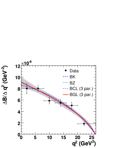
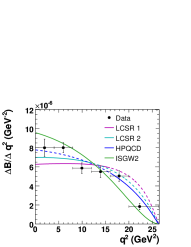
Refer to caption
Refer to caption
Figure 24: Measured Δ/Δq2ΔΔsuperscript𝑞2\Delta{\cal B}/\Delta q^{2} distribution for Bπν𝐵𝜋𝜈B\rightarrow\pi\ell\nu. The vertical error bars correspond to the combined statistical and systematic uncertainties. The positions of the data points have been adjusted to correspond to the mean q2superscript𝑞2q^{2} value in each bin, based on the quadratic BGL ansatz. Left: fits of four different form-factor parameterizations to the Δ/Δq2ΔΔsuperscript𝑞2\Delta{\cal B}/\Delta q^{2} data spectrum. The fit result for the BZ and BCL parameterizations are barely visible, since they overlap almost completely with the BGL result. The shaded band illustrates the uncertainty of the quadratic BGL fit to data. Right: shape comparisons of the data to various Bπν𝐵𝜋𝜈B\rightarrow\pi\ell\nu form-factor predictions (LCSR 1 ball_pi , LCSR 2 Siegen , HPQCD hpqcd04 , ISGW2 isgw2 ), which have been normalized to the measured total branching fraction. The extrapolations of the QCD predictions to the full q2superscript𝑞2q^{2} range are marked as dashed lines.
Refer to caption
Figure 25: (color online) Measured Δ/Δq2ΔΔsuperscript𝑞2\Delta{\cal B}/\Delta q^{2} distribution for Bρν𝐵𝜌𝜈B\rightarrow\rho\ell\nu. The inner and outer error bars correspond to the statistical uncertainty and the combined statistical and systematic uncertainty, respectively. The data are compared with the Bρν𝐵𝜌𝜈B\rightarrow\rho\ell\nu form-factor predictions from LCSR ball_rho and from the ISGW2 quark model isgw2 .

We compare the measured q2superscript𝑞2q^{2} spectra with the shapes predicted by form-factor calculations based on lattice QCD hpqcd04 , light-cone sum rules ball_pi ; Siegen , and the ISGW2 isgw2 relativistic quark model. Among the available calculations for Bπν𝐵𝜋𝜈B\rightarrow\pi\ell\nu decays, the HPQCD lattice calculation agrees best with the data. It should be noted that the LQCD predictions are only valid for q2>16GeV2superscript𝑞216superscriptGeV2q^{2}>16\mathrm{\,Ge\kern-1.00006ptV}^{2}, the earlier LCSR calculation (LCSR 1) for q2<16GeV2superscript𝑞216superscriptGeV2q^{2}<16\mathrm{\,Ge\kern-1.00006ptV}^{2}, and the more recent LCSR calculation (LCSR 2) for q2<12GeV2superscript𝑞212superscriptGeV2q^{2}<12\mathrm{\,Ge\kern-1.00006ptV}^{2}; their extrapolation is impacted by sizable uncertainties.

In Table 11 and Figure 25 we present the results of the fits to the Bρν𝐵𝜌𝜈B\rightarrow\rho\ell\nu samples. The LCSR calculation and the ISGW2 model are in good agreement with the data. However, the errors of the measured Bρν𝐵𝜌𝜈B\rightarrow\rho\ell\nu  partial branching fractions are relatively large, at the level of 15-30%, depending on the q2superscript𝑞2q^{2} interval.

It should be noted that the theoretical calculations differ most for low and high q2superscript𝑞2q^{2}. In these regions of phase space, the measurements are impacted significantly by higher levels of backgrounds, specifically continuum events at low q2superscript𝑞2q^{2} and other BXuν𝐵subscript𝑋𝑢𝜈B\rightarrow X_{u}\ell\nu decays that are difficult to separate from the signal modes at higher q2superscript𝑞2q^{2}. These two background sources have been examined in detail, and the uncertainties in their normalization and shape are included in the systematic uncertainties. For the inclusive BXuν𝐵subscript𝑋𝑢𝜈B\rightarrow X_{u}\ell\nu background, the q2superscript𝑞2q^{2} and the hadronic mass spectra are derived from theoretical predictions that depend on non-perturbative parameters that are not well measured moments . For Bρν𝐵𝜌𝜈B\rightarrow\rho\ell\nu the correlation between the signal and the BXuν𝐵subscript𝑋𝑢𝜈B\rightarrow X_{u}\ell\nu background is so large that they cannot both be fitted simultaneously. Thus the BXuν𝐵subscript𝑋𝑢𝜈B\rightarrow X_{u}\ell\nu background scale factor and shape are fixed to the MC predictions, which have large uncertainties. MC studies indicate that this may introduce a bias affecting the signal yield. The stated errors account for this potential bias.

VIII.3 Determination of |𝑽𝒖𝒃|subscript𝑽𝒖𝒃|V_{ub}|

We choose two different approaches to determine the magnitude of the CKM matrix element Vubsubscript𝑉𝑢𝑏V_{ub}.

First, we use the traditional method to derive |Vub|subscript𝑉𝑢𝑏|V_{ub}|. As in previous publications pilnu_jochen ; pilnu_cleo ; pilnu_cote ; pilnu_babar_tag ; pilnu_belle_tag , we combine the measured partial branching fractions with integrals of the form-factor calculations over a certain q2superscript𝑞2q^{2} range using the relation

|Vub|=Δ(qmin2,qmax2)τ0Δζ(qmin2,qmax2),subscript𝑉𝑢𝑏Δsubscriptsuperscript𝑞2𝑚𝑖𝑛subscriptsuperscript𝑞2𝑚𝑎𝑥subscript𝜏0Δ𝜁subscriptsuperscript𝑞2𝑚𝑖𝑛subscriptsuperscript𝑞2𝑚𝑎𝑥|V_{ub}|=\sqrt{\frac{\Delta{\cal B}(q^{2}_{min},q^{2}_{max})}{\tau_{0}\ \Delta\zeta(q^{2}_{min},q^{2}_{max})}}\ , (34)

where τ0=(1.530±0.009)subscript𝜏0plus-or-minus1.5300.009\tau_{0}=(1.530\pm 0.009) ps is the B0superscript𝐵0B^{0} lifetime and ΔζΔ𝜁\Delta\zeta is defined as

Δζ(qmin2,qmax2)=GF224π3qmin2qmax2pπ3|f+(q2)|2𝑑q2.Δ𝜁subscriptsuperscript𝑞2𝑚𝑖𝑛subscriptsuperscript𝑞2𝑚𝑎𝑥subscriptsuperscript𝐺2𝐹24superscript𝜋3superscriptsubscriptsubscriptsuperscript𝑞2𝑚𝑖𝑛subscriptsuperscript𝑞2𝑚𝑎𝑥superscriptsubscript𝑝𝜋3superscriptsubscript𝑓superscript𝑞22differential-dsuperscript𝑞2\Delta\zeta(q^{2}_{min},q^{2}_{max})=\frac{G^{2}_{F}}{24\pi^{3}}\int\limits_{q^{2}_{min}}^{q^{2}_{max}}p_{\pi}^{3}|f_{+}(q^{2})|^{2}dq^{2}\ . (35)

The values of ΔζΔ𝜁\Delta\zeta are derived from theoretical form-factor calculations for different q2superscript𝑞2q^{2} ranges. Table 13 summarizes the ΔζΔ𝜁\Delta\zeta values, the partial branching fractions and the |Vub|subscript𝑉𝑢𝑏|V_{ub}| results.

Table 13: |Vub|subscript𝑉𝑢𝑏|V_{ub}| derived from Bπν𝐵𝜋𝜈B\rightarrow\pi\ell\nu and Bρν𝐵𝜌𝜈B\rightarrow\rho\ell\nu decays for various q2superscript𝑞2q^{2} regions and form-factor calculations. Quoted errors are experimental uncertainties and theoretical uncertainties of the form-factor integral ΔζΔ𝜁\Delta\zeta. No uncertainties on ΔζΔ𝜁\Delta\zeta for Bρν𝐵𝜌𝜈B\rightarrow\rho\ell\nu are given in Refs. ball_rho and isgw2 .
q2superscript𝑞2q^{2} Range ΔΔ\Delta{\cal B} ΔζΔ𝜁\Delta\zeta |Vub|subscript𝑉𝑢𝑏|V_{ub}|
(GeV2superscriptGeV2\mathrm{\,Ge\kern-1.00006ptV}^{2}) (10-4) (ps-1) (10-3)
Bπν𝐵𝜋𝜈B\rightarrow\pi\ell\nu
LCSR 1 ball_pi 0160160-16 1.10±0.07plus-or-minus1.100.071.10\pm 0.07 5.44±1.43plus-or-minus5.441.435.44{\pm}1.43 3.63±0.120.40+0.59plus-or-minus3.63subscriptsuperscript0.120.590.403.63\pm 0.12^{+0.59}_{-0.40}
LCSR 2 Siegen 0120120-12 0.88±0.06plus-or-minus0.880.060.88\pm 0.06 4.000.95+1.01subscriptsuperscript4.001.010.954.00^{+1.01}_{-0.95} 3.78±0.130.40+0.55plus-or-minus3.78subscriptsuperscript0.130.550.403.78\pm 0.13^{+0.55}_{-0.40}
HPQCD hpqcd04 1626.41626.416-26.4 0.32±0.03plus-or-minus0.320.030.32\pm 0.03 2.02±0.55plus-or-minus2.020.552.02{\pm}0.55 3.21±0.170.36+0.55plus-or-minus3.21subscriptsuperscript0.170.550.363.21\pm 0.17^{+0.55}_{-0.36}
Bρν𝐵𝜌𝜈B\rightarrow\rho\ell\nu
LCSR ball_rho 016.0016.00-16.0 1.48±0.28plus-or-minus1.480.281.48\pm 0.28 13.7913.7913.79 2.75±0.24plus-or-minus2.750.242.75\pm 0.24
ISGW2 isgw2 020.3020.30-20.3 1.75±0.31plus-or-minus1.750.311.75\pm 0.31 14.2014.2014.20 2.83±0.24plus-or-minus2.830.242.83\pm 0.24

For Bρν𝐵𝜌𝜈B\rightarrow\rho\ell\nu, values of ΔζΔ𝜁\Delta\zeta are taken from the LCSR calculation in the range q2<16GeVsuperscript𝑞216GeVq^{2}<16\mathrm{\,Ge\kern-1.00006ptV} and the quark model predictions of ISGW2 over the full q2superscript𝑞2q^{2} range. The results are also presented in Table 13. Estimates of the uncertainties for ΔζΔ𝜁\Delta\zeta are not given in Refs. ball_rho and isgw2 .

Second, we perform a simultaneous fit to the most recent lattice results and BABAR data to make best use of the available information on the form factor from data (shape) and theory (shape and normalization). A fit of this kind was first presented by the FNAL/MILC Collaboration fnal09 using the earlier BABAR results on B0π+νsuperscript𝐵0superscript𝜋superscript𝜈B^{0}\rightarrow\pi^{-}\ell^{+}\nu decays pilnu_cote .

To perform this fit, we translate the f+(q2)subscript𝑓superscript𝑞2f_{+}(q^{2}) predictions from LQCD to 1/(τ0|Vub)|2)Δ/Δq21/(\tau_{0}|V_{ub})|^{2})\Delta{\cal B}/\Delta{q^{2}}. We simultaneously fit this distribution and the Δ/Δq2ΔΔsuperscript𝑞2\Delta{\cal B}/\Delta{q^{2}} distribution from data as a function of q2superscript𝑞2q^{2}. We use the BGL form-factor parameterization as the fit function, with the additional normalization parameter anorm=τ0|Vub|2subscript𝑎normsubscript𝜏0superscriptsubscript𝑉𝑢𝑏2a_{\rm norm}=\tau_{0}|V_{ub}|^{2}, which allows us to determine |Vub|subscript𝑉𝑢𝑏|V_{ub}| from the relative normalization of data and LQCD predictions.

The χ2superscript𝜒2\chi^{2} for this fit is given by

χ2superscript𝜒2\displaystyle\chi^{2} =\displaystyle= χ2(data)+χ2(lattice)superscript𝜒2datasuperscript𝜒2lattice\displaystyle\chi^{2}(\rm data)+\chi^{2}(\rm lattice) (36)
=\displaystyle= i,j=1NbinsΔidata(Vijdata)1Δjdatasuperscriptsubscript𝑖𝑗1subscript𝑁binssuperscriptsubscriptΔ𝑖datasuperscriptsuperscriptsubscript𝑉𝑖𝑗data1superscriptsubscriptΔ𝑗data\displaystyle\sum\limits_{i,j=1}^{N_{\rm bins}}\Delta_{i}^{\rm data}\ (V_{ij}^{\rm data})^{-1}\Delta_{j}^{\rm data}
+\displaystyle+ l,m=1NpointsΔllat(Vlmlat)1Δmlatsuperscriptsubscript𝑙𝑚1subscript𝑁pointssuperscriptsubscriptΔ𝑙latsuperscriptsuperscriptsubscript𝑉𝑙𝑚lat1superscriptsubscriptΔ𝑚lat\displaystyle\sum\limits_{l,m=1}^{N_{\rm points}}\Delta_{l}^{\rm lat}\ (V_{lm}^{\rm lat})^{-1}\Delta_{m}^{\rm lat}

where

ΔidatasuperscriptsubscriptΔ𝑖data\displaystyle\Delta_{i}^{\rm data} =\displaystyle= (ΔBΔq2)idata1Δqi2Δqi2g(q2;α)𝑑q2,subscriptsuperscriptΔ𝐵Δsuperscript𝑞2data𝑖1Δsubscriptsuperscript𝑞2𝑖subscriptΔsubscriptsuperscript𝑞2𝑖𝑔superscript𝑞2𝛼differential-dsuperscript𝑞2\displaystyle\left(\frac{\Delta B}{\Delta q^{2}}\right)^{\rm data}_{i}-\frac{1}{\Delta q^{2}_{i}}\int\limits_{\Delta q^{2}_{i}}g(q^{2};\alpha)dq^{2}\ , (37)
ΔllatsuperscriptsubscriptΔ𝑙lat\displaystyle\Delta_{l}^{\rm lat} =\displaystyle= GF224π3pπ3(ql2)|f+lat(ql2)|2g(ql2;α)subscriptsuperscript𝐺2𝐹24superscript𝜋3superscriptsubscript𝑝𝜋3subscriptsuperscript𝑞2𝑙superscriptsuperscriptsubscript𝑓latsubscriptsuperscript𝑞2𝑙2𝑔subscriptsuperscript𝑞2𝑙𝛼\displaystyle\frac{G^{2}_{F}}{24\pi^{3}}p_{\pi}^{3}(q^{2}_{l})|f_{+}^{\rm lat}(q^{2}_{l})|^{2}-g(q^{2}_{l};\alpha) (38)

and

g(q2;α)𝑔superscript𝑞2𝛼\displaystyle g(q^{2};\alpha) =\displaystyle= GF224π3pπ3(q2)|f+(q2)|2subscriptsuperscript𝐺2𝐹24superscript𝜋3superscriptsubscript𝑝𝜋3superscript𝑞2superscriptsubscript𝑓superscript𝑞22\displaystyle\frac{G^{2}_{F}}{24\pi^{3}}p_{\pi}^{3}(q^{2})|f_{+}(q^{2})|^{2} (41)
×\displaystyle\times {anormfor data1for LQCD,casessubscript𝑎normfor data1for LQCD\displaystyle\left\{\begin{array}[]{cl}a_{\rm norm}&\mbox{for data}\\ 1&\mbox{for LQCD}\end{array}\right.,
f+(q2)subscript𝑓superscript𝑞2\displaystyle f_{+}(q^{2}) =\displaystyle= 1𝒫(q2)ϕ(q2,q02)k=0kmaxak(q02)[z(q2,q02)]k.1𝒫superscript𝑞2italic-ϕsuperscript𝑞2subscriptsuperscript𝑞20superscriptsubscript𝑘0subscript𝑘𝑚𝑎𝑥subscript𝑎𝑘subscriptsuperscript𝑞20superscriptdelimited-[]𝑧superscript𝑞2subscriptsuperscript𝑞20𝑘\displaystyle\frac{1}{{\cal P}(q^{2})\phi(q^{2},q^{2}_{0})}\sum_{k=0}^{k_{max}}a_{k}(q^{2}_{0})[z(q^{2},q^{2}_{0})]^{k}. (42)

Here (ΔB/Δq2)datasuperscriptΔ𝐵Δsuperscript𝑞2data(\Delta B/\Delta q^{2})^{\rm data} is the measured spectrum, f+lat(ql2)superscriptsubscript𝑓latsuperscriptsubscript𝑞𝑙2f_{+}^{\rm lat}(q_{l}^{2}) are the form-factor predictions from LQCD, and (Vijdata)1superscriptsuperscriptsubscript𝑉𝑖𝑗data1(V_{ij}^{\rm data})^{-1} and (Vijlat)1superscriptsuperscriptsubscript𝑉𝑖𝑗lat1(V_{ij}^{\rm lat})^{-1} are the corresponding inverse covariance matrices for (ΔB/Δq2)datasuperscriptΔ𝐵Δsuperscript𝑞2data(\Delta B/\Delta q^{2})^{\rm data} and GF2/(24π3)pπ3(ql2)|f+lat(ql2)|2subscriptsuperscript𝐺2𝐹24superscript𝜋3superscriptsubscript𝑝𝜋3subscriptsuperscript𝑞2𝑙superscriptsuperscriptsubscript𝑓latsubscriptsuperscript𝑞2𝑙2G^{2}_{F}/(24\pi^{3})p_{\pi}^{3}(q^{2}_{l})|f_{+}^{\rm lat}(q^{2}_{l})|^{2}, respectively. The set of free parameters α𝛼\alpha of the fit function g(q2;α)𝑔superscript𝑞2𝛼g(q^{2};\alpha) contains the coefficients aksubscript𝑎𝑘a_{k} of the BGL parameterization and the normalization parameter anormsubscript𝑎norma_{\rm norm}.

From the FNAL/MILC fnal09 lattice calculations, we use only subsets with six, four or three of the twelve predictions at different values of q2superscript𝑞2q^{2}, since neighboring points are very strongly correlated. All chosen subsets of LQCD points contain the point at lowest q2superscript𝑞2q^{2}. It has been checked that alternative choices of subsets give compatible results. From the HPQCD hpqcd04 lattice calculations, we use only the point at lowest q2superscript𝑞2q^{2} since the correlation matrix for the four predicted points is not available. For comparison, we also perform the corresponding fit using only the point at lowest q2superscript𝑞2q^{2} from FNAL/MILC. The data, the lattice predictions, and the fitted functions are shown in Figure 26. Table 14 shows the numerical results of the fit.
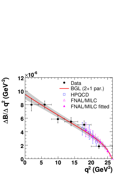
Refer to caption Refer to caption
Figure 26: (color online) Simultaneous fits of the BGL parameterization to data (solid points with vertical error bars representing the total experimental uncertainties) and to four of the twelve points of the FNAL/MILC lattice prediction (magenta, closed triangles). Left: linear (2+1-parameter) BGL fit, right: quadratic (3+1-parameter) BGL fit. The LQCD results are rescaled to the data according to the |Vub|subscript𝑉𝑢𝑏|V_{ub}| value obtained in the fit. The shaded band illustrates the uncertainty of the fitted function. For comparison, the HPQCD (blue, open squares) lattice results are also shown. They are used in an alternate fit.
Table 14: Results of simultaneous fits to data and LQCD calculations, based on the linear or quadratic BGL parameterizations. |Vub|subscript𝑉𝑢𝑏|V_{ub}| is determined from the relative normalization of data and theory prediction.
Parameterization Input χ2superscript𝜒2\chi^{2}/ndf Prob(χ2superscript𝜒2\chi^{2}/ndf) Fit parameters
BGL (2+1 par.) Data 18.2/918.2918.2/9 0.033 a0=(2.07±0.21)×102subscript𝑎0plus-or-minus2.070.21superscript102a_{0}=(2.07\pm 0.21)\times 10^{-2}
+ FNAL/MILC a1/a0=0.78±0.22subscript𝑎1subscript𝑎0plus-or-minus0.780.22a_{1}/a_{0}=-0.78\pm 0.22
(6 points) |Vub|=(3.04±0.38)×103subscript𝑉𝑢𝑏plus-or-minus3.040.38superscript103|V_{ub}|=(3.04\pm 0.38)\times 10^{-3}
BGL (2+1 par.) Data 7.1/77.177.1/7 0.415 a0=(2.16±0.19)×102subscript𝑎0plus-or-minus2.160.19superscript102a_{0}=(2.16\pm 0.19)\times 10^{-2}
+ FNAL/MILC a1/a0=0.93±0.20subscript𝑎1subscript𝑎0plus-or-minus0.930.20a_{1}/a_{0}=-0.93\pm 0.20
(4 points) |Vub|=(2.99±0.32)×103subscript𝑉𝑢𝑏plus-or-minus2.990.32superscript103|V_{ub}|=(2.99\pm 0.32)\times 10^{-3}
BGL (2+1 par.) Data 6.8/66.866.8/6 0.341 a0=(2.17±0.19)×102subscript𝑎0plus-or-minus2.170.19superscript102a_{0}=(2.17\pm 0.19)\times 10^{-2}
+ FNAL/MILC a1/a0=0.93±0.20subscript𝑎1subscript𝑎0plus-or-minus0.930.20a_{1}/a_{0}=-0.93\pm 0.20
(3 points) |Vub|=(2.97±0.32)×103subscript𝑉𝑢𝑏plus-or-minus2.970.32superscript103|V_{ub}|=(2.97\pm 0.32)\times 10^{-3}
BGL (2+1 par.) Data 6.6/46.646.6/4 0.156 a0=(2.23±0.26)×102subscript𝑎0plus-or-minus2.230.26superscript102a_{0}=(2.23\pm 0.26)\times 10^{-2}
+ FNAL/MILC a1/a0=0.94±0.20subscript𝑎1subscript𝑎0plus-or-minus0.940.20a_{1}/a_{0}=-0.94\pm 0.20
(1 point) |Vub|=(2.90±0.36)×103subscript𝑉𝑢𝑏plus-or-minus2.900.36superscript103|V_{ub}|=(2.90\pm 0.36)\times 10^{-3}
BGL (2+1 par.) Data 6.6/46.646.6/4 0.156 a0=(2.19±0.23)×102subscript𝑎0plus-or-minus2.190.23superscript102a_{0}=(2.19\pm 0.23)\times 10^{-2}
+ HPQCD a1/a0=0.94±0.20subscript𝑎1subscript𝑎0plus-or-minus0.940.20a_{1}/a_{0}=-0.94\pm 0.20
(1 point) |Vub|=(2.94±0.34)×103subscript𝑉𝑢𝑏plus-or-minus2.940.34superscript103|V_{ub}|=(2.94\pm 0.34)\times 10^{-3}
BGL (3+1 par.) Data 9.8/89.889.8/8 0.276 a0=(2.31±0.20)×102subscript𝑎0plus-or-minus2.310.20superscript102a_{0}=(2.31\pm 0.20)\times 10^{-2}
+ FNAL/MILC a1/a0=0.71±0.19subscript𝑎1subscript𝑎0plus-or-minus0.710.19a_{1}/a_{0}=-0.71\pm 0.19
(6 points) a2/a0=2.33±0.84subscript𝑎2subscript𝑎0plus-or-minus2.330.84a_{2}/a_{0}=-2.33\pm 0.84
|Vub|=(2.87±0.28)×103subscript𝑉𝑢𝑏plus-or-minus2.870.28superscript103|V_{ub}|=(2.87\pm 0.28)\times 10^{-3}
BGL (3+1 par.) Data 6.6/66.666.6/6 0.355 a0=(2.22±0.21)×102subscript𝑎0plus-or-minus2.220.21superscript102a_{0}=(2.22\pm 0.21)\times 10^{-2}
+ FNAL/MILC a1/a0=0.86±0.23subscript𝑎1subscript𝑎0plus-or-minus0.860.23a_{1}/a_{0}=-0.86\pm 0.23
(4 points) a2/a0=0.97±1.36subscript𝑎2subscript𝑎0plus-or-minus0.971.36a_{2}/a_{0}=-0.97\pm 1.36
|Vub|=(2.95±0.31)×103subscript𝑉𝑢𝑏plus-or-minus2.950.31superscript103|V_{ub}|=(2.95\pm 0.31)\times 10^{-3}
BGL (3+1 par.) Data 6.3/56.356.3/5 0.279 a0=(2.24±0.22)×102subscript𝑎0plus-or-minus2.240.22superscript102a_{0}=(2.24\pm 0.22)\times 10^{-2}
+ FNAL/MILC a1/a0=0.84±0.23subscript𝑎1subscript𝑎0plus-or-minus0.840.23a_{1}/a_{0}=-0.84\pm 0.23
(3 points) a2/a0=1.01±1.40subscript𝑎2subscript𝑎0plus-or-minus1.011.40a_{2}/a_{0}=-1.01\pm 1.40
|Vub|=(2.93±0.31)×103subscript𝑉𝑢𝑏plus-or-minus2.930.31superscript103|V_{ub}|=(2.93\pm 0.31)\times 10^{-3}
BGL (3+1 par.) Data 6.3/36.336.3/3 0.100 a0=(2.24±0.26)×102subscript𝑎0plus-or-minus2.240.26superscript102a_{0}=(2.24\pm 0.26)\times 10^{-2}
+ FNAL/MILC a1/a0=0.82±0.29subscript𝑎1subscript𝑎0plus-or-minus0.820.29a_{1}/a_{0}=-0.82\pm 0.29
(1 point) a2/a0=1.14±1.81subscript𝑎2subscript𝑎0plus-or-minus1.141.81a_{2}/a_{0}=-1.14\pm 1.81
|Vub|=(2.92±0.37)×103subscript𝑉𝑢𝑏plus-or-minus2.920.37superscript103|V_{ub}|=(2.92\pm 0.37)\times 10^{-3}
BGL (3+1 par.) Data 6.3/36.336.3/3 0.100 a0=(2.19±0.23)×102subscript𝑎0plus-or-minus2.190.23superscript102a_{0}=(2.19\pm 0.23)\times 10^{-2}
+ HPQCD a1/a0=0.82±0.29subscript𝑎1subscript𝑎0plus-or-minus0.820.29a_{1}/a_{0}=-0.82\pm 0.29
(1 point) a2/a0=1.14±1.81subscript𝑎2subscript𝑎0plus-or-minus1.141.81a_{2}/a_{0}=-1.14\pm 1.81
|Vub|=(2.99±0.35)×103subscript𝑉𝑢𝑏plus-or-minus2.990.35superscript103|V_{ub}|=(2.99\pm 0.35)\times 10^{-3}

For the nominal fit we use the subset with four FNAL/MILC points and assume a quadratic BGL parameterization. We refer to this fit as 3+1-parameter BGL fit (three coefficients aksubscript𝑎𝑘a_{k} and the normalization parameter anormsubscript𝑎norma_{\rm norm}). As can be seen in Table 12 for the fit to data alone, the data are well described by a linear function with the normalization a0subscript𝑎0a_{0} and a slope a1/a0subscript𝑎1subscript𝑎0a_{1}/a_{0}. This indicates that most of the variation of the form factor is due to well-understood QCD effects that are parameterized by the functions 𝒫(q2)𝒫superscript𝑞2{\cal P}(q^{2}) and ϕ(q2,q02)italic-ϕsuperscript𝑞2superscriptsubscript𝑞02\phi(q^{2},q_{0}^{2}) in the BGL parameterization. If we include a curvature term in the fit, the slope a1/a0=0.82±0.29subscript𝑎1subscript𝑎0plus-or-minus0.820.29a_{1}/a_{0}=-0.82\pm 0.29 is fully consistent with the linear fit; the curvature a2/a0subscript𝑎2subscript𝑎0a_{2}/a_{0} is negative and consistent with zero. Since the z𝑧z distribution is almost linear, we also perform a linear fit (2+1-parameter BGL fit) for comparison. The results of the linear fits are also shown in Table 14.

The simultaneous fits provide very similar results, both for the BGL expansion coefficients, which determine the shape of the spectrum, and for |Vub|subscript𝑉𝑢𝑏|V_{ub}|. The fitted values for the form-factor parameters are very similar to those obtained from the fits to data alone. This is not surprising, since the data dominate the fit results. Unfortunately the decay rate is lowest and the experimental errors are largest at large q2superscript𝑞2q^{2}, where the lattice calculation can make predictions. We obtain from these simultaneous fits

|Vub|subscript𝑉𝑢𝑏\displaystyle|V_{ub}| =\displaystyle= (2.87±0.28)×103FNAL/MILC(6points),plus-or-minus2.870.28superscript103FNALMILC6points\displaystyle(2.87\pm 0.28)\times 10^{-3}\quad{\rm FNAL/MILC~{}(6~{}points)}\ ,
|Vub|subscript𝑉𝑢𝑏\displaystyle|V_{ub}| =\displaystyle= (2.95±0.31)×103FNAL/MILC(4points),plus-or-minus2.950.31superscript103FNALMILC4points\displaystyle(2.95\pm 0.31)\times 10^{-3}\quad{\rm FNAL/MILC~{}(4~{}points)}\ ,
|Vub|subscript𝑉𝑢𝑏\displaystyle|V_{ub}| =\displaystyle= (2.93±0.31)×103FNAL/MILC(3points),plus-or-minus2.930.31superscript103FNALMILC3points\displaystyle(2.93\pm 0.31)\times 10^{-3}\quad{\rm FNAL/MILC~{}(3~{}points)}\ ,
|Vub|subscript𝑉𝑢𝑏\displaystyle|V_{ub}| =\displaystyle= (2.92±0.37)×103FNAL/MILC(1point),plus-or-minus2.920.37superscript103FNALMILC1point\displaystyle(2.92\pm 0.37)\times 10^{-3}\quad{\rm FNAL/MILC~{}(1~{}point)}\ ,
|Vub|subscript𝑉𝑢𝑏\displaystyle|V_{ub}| =\displaystyle= (2.99±0.35)×103HPQCD(1point),plus-or-minus2.990.35superscript103HPQCD1point\displaystyle(2.99\pm 0.35)\times 10^{-3}\quad{\rm HPQCD~{}(1~{}point)}\ ,

where the stated error is the combined experimental and theoretical error obtained from the fit. The coefficients aksubscript𝑎𝑘a_{k} are significantly smaller than 1, as predicted. The sum of the squares of the first two coefficients, k=01ak2=(0.85±0.20)×103superscriptsubscript𝑘01superscriptsubscript𝑎𝑘2plus-or-minus0.850.20superscript103\sum_{k=0}^{1}a_{k}^{2}=(0.85\pm 0.20)\times 10^{-3}, is consistent with the tighter bounds set by Becher and Hill BHill .

Since the total error of 10% on |Vub|subscript𝑉𝑢𝑏|V_{ub}| results from the simultaneous fit to data and LQCD predictions, it is non-trivial to separate the error into contributions from experiment and theory. We have estimated that the error contains contributions of 3%percent33\% from the branching-fraction measurement, 5%percent55\% from the shape of the q2superscript𝑞2q^{2} spectrum determined from data, and 8.5%percent8.58.5\% from the form-factor normalization obtained from theory.

We study the effect of variations of the isospin relations imposed in the combined four-mode fit as stated in Eqs. 30. These relations are not expected to be exact, though the comparison of the single-mode fit results provides no indication for isospin breaking. The isospin-breaking effects are primarily due to π0ηsuperscript𝜋0𝜂\pi^{0}-\eta and ρ0ωsuperscript𝜌0𝜔\rho^{0}-\omega mixing in B+π0+νsuperscript𝐵superscript𝜋0superscript𝜈B^{+}\rightarrow\pi^{0}\ell^{+}\nu and B+ρ0+νsuperscript𝐵superscript𝜌0superscript𝜈B^{+}\rightarrow\rho^{0}\ell^{+}\nu decays, respectively. They are expected to increase the branching fractions of the B+superscript𝐵B^{+} relative to the B0superscript𝐵0B^{0} meson. Given the masses and widths of the mesons involved, the impact of π0ηsuperscript𝜋0𝜂\pi^{0}-\eta mixing is expected to be smaller than that of ρ0ωsuperscript𝜌0𝜔\rho^{0}-\omega mixing.

Detailed calculations have been performed to correct form-factor measurements and to extract Vussubscript𝑉𝑢𝑠V_{us} from semileptonic decays of charged and neutral kaons ckmbook . These calculations account for isospin breaking due to π0ηsuperscript𝜋0𝜂\pi^{0}-\eta mixing and should also be applicable to B+π0+νsuperscript𝐵superscript𝜋0superscript𝜈B^{+}\rightarrow\pi^{0}\ell^{+}\nu decays. For B+π0+νsuperscript𝐵superscript𝜋0superscript𝜈B^{+}\rightarrow\pi^{0}\ell^{+}\nu decays the effect is expected to be smaller by a factor of three, i.e., the predicted increase is (1.5±0.2)plus-or-minus1.50.2(1.5\pm 0.2)vincenzo . For B+ρ0+νsuperscript𝐵superscript𝜌0superscript𝜈B^{+}\rightarrow\rho^{0}\ell^{+}\nu decays, calculations have not been carried out to the same precision. Based on the change in the π+πsuperscript𝜋superscript𝜋\pi^{+}\pi^{-} rate at the peak of the ρ𝜌\rho mass distribution, the branching fraction is predicted to increase by as much as 34% lopez . However, an integration over the resonances weighted by the proper Breit-Wigner function and taking into account the masses and finite ρ𝜌\rho and ω𝜔\omega widths results in a much smaller effect, an increase in the π+πsuperscript𝜋superscript𝜋\pi^{+}\pi^{-} branching fraction of 6% lange .

We have assessed the impact of changes in the ratios of the branching fractions for charged and neutral B𝐵B mesons on the extraction of the differential decay rates due to adjustments of the MC default branching fractions of the B+superscript𝐵B^{+} decays in the combined four-mode fit. For a 1.5% increase in the B+π0+νsuperscript𝐵superscript𝜋0superscript𝜈B^{+}\rightarrow\pi^{0}\ell^{+}\nu branching fraction, the fitted Bπν𝐵𝜋𝜈B\rightarrow\pi\ell\nu partial branching fraction decreases by 0.5%, while the Bρν𝐵𝜌𝜈B\rightarrow\rho\ell\nu rate increases by less than 0.1%. A 6% increase in the B+ρ0+νsuperscript𝐵superscript𝜌0superscript𝜈B^{+}\rightarrow\rho^{0}\ell^{+}\nu branching fraction results in a decrease of the Bρν𝐵𝜌𝜈B\rightarrow\rho\ell\nu rate by 3.1% and a 0.14% increase for the fitted Bπν𝐵𝜋𝜈B\rightarrow\pi\ell\nu rate. We observe a partial compensation to the change in the simulated B+π0+νsuperscript𝐵superscript𝜋0superscript𝜈B^{+}\rightarrow\pi^{0}\ell^{+}\nu rate due to changes in the B+ρ0+νsuperscript𝐵superscript𝜌0superscript𝜈B^{+}\rightarrow\rho^{0}\ell^{+}\nu background contribution, and vice versa. The observed changes in the fitted yields depend linearly on the imposed branching-fraction changes and are independent of q2superscript𝑞2q^{2}.

For a 1.5%percent1.51.5\% variation of the B+π0+νsuperscript𝐵superscript𝜋0superscript𝜈B^{+}\rightarrow\pi^{0}\ell^{+}\nu branching fraction, the value for |Vub|subscript𝑉𝑢𝑏|V_{ub}| extracted from the measured Bπν𝐵𝜋𝜈B\rightarrow\pi\ell\nu spectrum decreases by 0.2%percent0.20.2\%. A +6%percent6+6\% variation of the B+ρ0+νsuperscript𝐵superscript𝜌0superscript𝜈B^{+}\rightarrow\rho^{0}\ell^{+}\nu branching fraction increases the value of |Vub|subscript𝑉𝑢𝑏|V_{ub}| extracted from the same measured spectrum by 0.3%percent0.30.3\%.

IX Conclusions

In summary, we have measured the exclusive branching fractions (B0π+ν{\cal B}(B^{0}\rightarrow\pi^{-}\ell^{+}\nu) and (B0ρ+ν{\cal B}(B^{0}\rightarrow\rho^{-}\ell^{+}\nu) as a function of q2superscript𝑞2q^{2} and have determined |Vub|subscript𝑉𝑢𝑏|V_{ub}| using recent form-factor calculations. We measure the total branching fractions, based on samples of charged and neutral B𝐵B mesons and isospin constraints, to be

(B0π+ν)superscript𝐵0superscript𝜋superscript𝜈\displaystyle{\cal B}(B^{0}\rightarrow\pi^{-}\ell^{+}\nu) =\displaystyle= (1.41±0.05±0.07)×104,plus-or-minus1.410.050.07superscript104\displaystyle(1.41\pm 0.05\pm 0.07)\times 10^{-4}\ ,
(B0ρ+ν)superscript𝐵0superscript𝜌superscript𝜈\displaystyle{\cal B}(B^{0}\rightarrow\rho^{-}\ell^{+}\nu) =\displaystyle= (1.75±0.15±0.27)×104,plus-or-minus1.750.150.27superscript104\displaystyle(1.75\pm 0.15\pm 0.27)\times 10^{-4}\ ,

where the first error is the statistical uncertainty of the fit employed to determine the signal and background yields and the second is the systematic uncertainty. The separate measurements of the branching fractions for charged and neutral B𝐵B mesons are consistent within errors with the assumed isospin relations,

(B0π+ν)(B+π0+ν)×2τ0τ+superscript𝐵0superscript𝜋superscript𝜈superscript𝐵superscript𝜋0superscript𝜈2subscript𝜏0subscript𝜏\displaystyle\frac{{\cal B}(B^{0}\rightarrow\pi^{-}\ell^{+}\nu)}{{\cal B}(B^{+}\rightarrow\pi^{0}\ell^{+}\nu)\times 2\frac{\tau_{0}}{\tau_{+}}} =\displaystyle= 1.03±0.09±0.06,plus-or-minus1.030.090.06\displaystyle 1.03\pm 0.09\pm 0.06\ ,
(B0ρ+ν)(B+ρ0+ν)×2τ0τ+superscript𝐵0superscript𝜌superscript𝜈superscript𝐵superscript𝜌0superscript𝜈2subscript𝜏0subscript𝜏\displaystyle\frac{{\cal B}(B^{0}\rightarrow\rho^{-}\ell^{+}\nu)}{{\cal B}(B^{+}\rightarrow\rho^{0}\ell^{+}\nu)\times 2\frac{\tau_{0}}{\tau_{+}}} =\displaystyle= 1.06±0.16±0.08.plus-or-minus1.060.160.08\displaystyle 1.06\pm 0.16\pm 0.08\ .

We have assessed the sensitivity of the combined branching-fraction measurements to isospin violations due to π0ηsuperscript𝜋0𝜂\pi^{0}-\eta and ρ0ωsuperscript𝜌0𝜔\rho^{0}-\omega mixing in B+superscript𝐵B^{+} decays. Based on the best estimates currently available, the impact on the branching fractions is small compared to the total systematic errors. We refrain from applying corrections, given the uncertainties in the size of the effects.

The measured branching fraction for Bπν𝐵𝜋𝜈B\rightarrow\pi\ell\nu is more precise than any previous measurement and agrees well with the current world average (B0π+ν)=(1.36±0.05±0.05)×104superscript𝐵0superscript𝜋superscript𝜈plus-or-minus1.360.050.05superscript104{\cal B}(B^{0}\rightarrow\pi^{-}\ell^{+}\nu)=(1.36\pm 0.05\pm 0.05)\times 10^{-4} HFAG2009 . The branching fraction for Bρν𝐵𝜌𝜈B\rightarrow\rho\ell\nu is also the most precise single measurement to date based on a large signal event sample, although the Belle Collaboration pilnu_belle_tag has reported a smaller systematic error (by a factor of two), based on a small signal sample of hadronically-tagged events pilnu_belle_tag . The Bρν𝐵𝜌𝜈B\rightarrow\rho\ell\nu branching fraction presented here is significantly lower (by about 2.5σ2.5𝜎2.5~{}\sigma) compared to the current world average (B0ρ+ν)=(2.77±0.18±0.16)×104superscript𝐵0superscript𝜌superscript𝜈plus-or-minus2.770.180.16superscript104{\cal B}(B^{0}\rightarrow\rho^{-}\ell^{+}\nu)=(2.77\pm 0.18\pm 0.16)\times 10^{-4} HFAG2009 . The dominant uncertainty of this Bρν𝐵𝜌𝜈B\rightarrow\rho\ell\nu measurement is due to the limited knowledge of the normalization and shape of the irreducible background from other BXuν𝐵subscript𝑋𝑢𝜈B\rightarrow X_{u}\ell\nu decays.

Within the sizable errors, the measured q2superscript𝑞2q^{2} spectrum for Bρν𝐵𝜌𝜈B\rightarrow\rho\ell\nu agrees well with the predictions from light-cone sum rules ball_rho and the ISGW2 isgw2 quark model. Neither of these calculations includes an estimate of their uncertainties. In the future, it will require much cleaner data samples and considerably better understanding of other BXuν𝐵subscript𝑋𝑢𝜈B\rightarrow X_{u}\ell\nu decays to achieve significant improvements in the measurements of the form factors in B𝐵B decays to vector mesons.

For Bπν𝐵𝜋𝜈B\rightarrow\pi\ell\nu decays, the measured q2superscript𝑞2q^{2} spectrum agrees best with the one predicted by the HPQCD lattice calculations hpqcd04 . The measurement of the differential decay rates is consistent with earlier BABAR measurements pilnu_jochen ; pilnu_cote within the stated errors, though the yield at low q2superscript𝑞2q^{2} is somewhat higher than previously measured. This results in a smaller value of αBKsubscript𝛼𝐵𝐾\alpha_{BK}, the parameter introduced by Becirevic and Kaidalov BK , namely αBK=0.31±0.09subscript𝛼𝐵𝐾plus-or-minus0.310.09\alpha_{BK}=0.31\pm 0.09. Using the BGL ansatz, we determine a value f+(0)|Vub|=(1.08±0.06)×103subscript𝑓0subscript𝑉𝑢𝑏plus-or-minus1.080.06superscript103f_{+}(0)|V_{ub}|=(1.08\pm 0.06)\times 10^{-3}, which is larger than the value, f+(0)|Vub|=(0.91±0.06±0.3)×103subscript𝑓0subscript𝑉𝑢𝑏plus-or-minus0.910.060.3superscript103f_{+}(0)|V_{ub}|=(0.91\pm 0.06\pm 0.3)\times 10^{-3} ball07 , based on the earlier BABAR decay rate measurement pilnu_cote and an average branching fraction of (1.37±0.06±0.07)×104plus-or-minus1.370.060.07superscript104(1.37\pm 0.06\pm 0.07)\times 10^{-4} HFAG2009 .

We determine the CKM matrix element |Vub|subscript𝑉𝑢𝑏|V_{ub}| using two different approaches. First, we use the traditional method to derive |Vub|subscript𝑉𝑢𝑏|V_{ub}| by combining the measured partial branching fractions with the form-factor predictions based on different QCD calculations. The results, presented in Table 13, agree within the sizable uncertainties of the form-factor predictions. For this approach we quote as a result the value of

|Vub|=(3.78±0.130.40+0.55)×103,subscript𝑉𝑢𝑏plus-or-minus3.78subscriptsuperscript0.130.550.40superscript103|V_{ub}|=(3.78\pm 0.13^{+0.55}_{-0.40})\times 10^{-3},

based on the most recent LCSR calculation for q2<12GeV2superscript𝑞212superscriptGeV2q^{2}<12\mathrm{\,Ge\kern-1.00006ptV}^{2}. Second, we extract |Vub|subscript𝑉𝑢𝑏|V_{ub}| from simultaneous fits to data and lattice predictions using the quadratic BGL parameterization for the whole q2superscript𝑞2q^{2} range. These fits to data and the two most recent lattice calculations by the FNAL/MILC fnal09 and HPQCD hpqcd04 Collaborations agree very well. We quote as a result the fitted value of

|Vub|=(2.95±0.31)×103,subscript𝑉𝑢𝑏plus-or-minus2.950.31superscript103|V_{ub}|=(2.95\pm 0.31)\times 10^{-3},

based on the normalization predicted by the FNAL/MILC Collaboration. The total error of 10% is dominated by the theory error of 8.5%. This value of |Vub|subscript𝑉𝑢𝑏|V_{ub}| is smaller by one standard deviation compared to the results of a combined fit to earlier BABAR measurements and the same recent FNAL/MILC lattice calculations fnal09 .

The values of |Vub|subscript𝑉𝑢𝑏|V_{ub}| presented here appear to be sensitive to the q2superscript𝑞2q^{2} range for which theory predictions and the measured spectrum can be compared. LCSR calculations are restricted to low values of q2superscript𝑞2q^{2} and result in values of |Vub|subscript𝑉𝑢𝑏|V_{ub}| in the range of (3.633.78)×1033.633.78superscript103(3.63-3.78)\times 10^{-3} with theoretical uncertainties of %11+16{}^{+16}_{-11}\% and experimental errors of 34%3percent43-4\%. LQCD predictions are available for q2>16GeV2superscript𝑞216superscriptGeV2q^{2}>16\mathrm{\,Ge\kern-1.00006ptV}^{2} and result in |Vub|subscript𝑉𝑢𝑏|V_{ub}| in the range of (2.953.21)×1032.953.21superscript103(2.95-3.21)\times 10^{-3} and experimental errors of 56%5percent65-6\% for both the traditional method and the simultaneous fit to LQCD predictions and the measured spectrum. This fit combines the measured shape of the spectrum over the full q2superscript𝑞2q^{2} range with the lattice QCD form-factor predictions at high q2superscript𝑞2q^{2} and results in a reduced theoretical uncertainty of 8.5%percent8.58.5\%, as compared to %11+17{}^{+17}_{-11}\% for the traditional method.

Both |Vub|subscript𝑉𝑢𝑏|V_{ub}| values quoted as results are also lower than most determinations of |Vub|subscript𝑉𝑢𝑏|V_{ub}| based on inclusive BXuν𝐵subscript𝑋𝑢𝜈B\rightarrow X_{u}\ell\nu decays, which are typically in the range (4.04.5)×1034.04.5superscript103(4.0-4.5)\times 10^{-3}. These inclusive measurements are very sensitive to the mass of the b𝑏b quark, which is extracted from fits to moments of inclusive BXcν𝐵subscript𝑋𝑐𝜈B\rightarrow X_{c}\ell\nu and BXsγ𝐵subscript𝑋𝑠𝛾B\rightarrow X_{s}\gamma decay distributions moments and depends on higher-order QCD corrections. Estimated theoretical uncertainties are typically 6%percent66\%.

Global fits constraining the parameters of the CKM unitarity triangle performed by the CKMfitter CKMfitter and UTfit UTfit Collaborations currently predict values for |Vub|subscript𝑉𝑢𝑏|V_{ub}| that fall between the two results presented here, |Vub|=3.510.16+0.14×10³subscript𝑉𝑢𝑏subscriptsuperscript3.510.140.16superscript103|V_{ub}|=3.51^{+0.14}_{-0.16}\times 10^{-3} and |Vub|=3.41±0.18×10³subscript𝑉𝑢𝑏plus-or-minus3.410.18superscript103|V_{ub}|=3.41\pm 0.18\times 10^{-3}, respectively.

To permit more stringent tests of the CKM framework and its consistency with the standard model of electroweak interactions, further reductions in the experimental and theoretical uncertainties will be necessary. For Bπν𝐵𝜋𝜈B\rightarrow\pi\ell\nu decays this will require a reduction in the statistical errors and improved detector hermeticity to more effectively reconstruct the neutrino, which will reduce backgrounds from all sources. Further improvements in the precision of lattice and other QCD calculations will also be beneficial.

X Acknowledgments

We would like to thank A. Khodjamirian, A. Kronfeld, P. Mackenzie, T. Mannel, J. Shigemitsu, and R. Van de Water for their help with theoretical form-factor calculations. We are grateful for the extraordinary contributions of our PEP-II colleagues in achieving the excellent luminosity and machine conditions that have made this work possible. The success of this project also relies critically on the expertise and dedication of the computing organizations that support BABAR. The collaborating institutions wish to thank SLAC for its support and the kind hospitality extended to them. This work is supported by the US Department of Energy and National Science Foundation, the Natural Sciences and Engineering Research Council (Canada), the Commissariat à l’Energie Atomique and Institut National de Physique Nucléaire et de Physique des Particules (France), the Bundesministerium für Bildung und Forschung and Deutsche Forschungsgemeinschaft (Germany), the Istituto Nazionale di Fisica Nucleare (Italy), the Foundation for Fundamental Research on Matter (The Netherlands), the Research Council of Norway, the Ministry of Education and Science of the Russian Federation, Ministerio de Ciencia e Innovación (Spain), and the Science and Technology Facilities Council (United Kingdom). Individuals have received support from the Marie-Curie IEF program (European Union), the A. P. Sloan Foundation (USA) and the Binational Science Foundation (USA-Israel).

References

  • (1) BABAR Collaboration, B. Aubert et al., Phys. Rev. Lett. 99, 171803 (2007).
  • (2) Belle Collaboration, K. F. Chen et al., Phys. Rev. Lett. 98, 031802 (2007).
  • (3) N. Cabibbo, Phys. Lett. 10, 531 (1963); M. Kobayashi and T. Maskawa, Prog. Theor. Phys. 49, 652 (1973).
  • (4) R. Kowalewski and T. Mannel in Review of Particle Physics, Phys. Lett. B667, 951 (2008).
  • (5) Charge conjugate decay modes are implicitly included.
  • (6) BABAR Collaboration, B. Aubert et al., Phys. Rev. D72, 051102 (2005).
  • (7) Particle Data Group, C. Amsler et al., Phys. Lett. B667, 1 (2008).
  • (8) CLEO Collaboration, S. B. Athar et al., Phys. Rev. D68, 072003 (2003); N. E. Adam et al., Phys. Rev. Lett. 99, 041802 (2007).
  • (9) BABAR Collaboration, B. Aubert et al., Phys. Rev. Lett. 98, 091801 (2007).
  • (10) BABAR Collaboration, B. Aubert et al., Phys. Rev. Lett. 97, 211801 (2006); Phys. Rev. Lett. 101, 081801 (2008).
  • (11) Belle Collaboration, T. Hokuue et al., Phys. Lett. B648, 139 (2007); Belle Collaboration, I. Adachi et al., Measurement of exclusive BXuν𝐵subscript𝑋𝑢𝜈B\rightarrow X_{u}\ell\nu decays using full-reconstruction tagging at Belle, e-Print: arXiv:0812:1414 (2008).
  • (12) M. Neubert, Physics Reports 245, 259 (1994).
  • (13) J. D. Richman and P. R. Burchat, Rev. Mod. Phys. 67, 893 (1995).
  • (14) N. Isgur, D. Scora, B. Grinstein, and M. B. Wise, Phys. Rev. D39, 799 (1989); D. Scora, N. Isgur, Phys. Rev. D52, 2783 (1995).
  • (15) P. Ball and R. Zwicky, JHEP 0110, 019 (2001); Phys. Rev. D71, 014015 (2005).
  • (16) P. Ball, Phys. Lett. B644, 38 (2007).
  • (17) P. Ball and V. M. Braun, Phys. Rev. D58, 094016 (1998); P. Ball and R. Zwicky, Phys. Rev. D71, 014029 (2005).
  • (18) P. Ball and G. Jones, JHEP 08, 025 (2007).
  • (19) G. Duplancic, A. Khodjamirian, T. Mannel, B. Melic and N. Offen, JHEP 804, 14 (2008); private communication, A. Khodjamirian (2010). The extrapolation of this calculation to higher q2superscript𝑞2q^{2} uses a BK parameterization with shape parameter α=0.53𝛼0.53\alpha=0.53, based on a fit to earlier BABAR data.
  • (20) Fermilab Lattice Collaboration, Aida X. El-Khadra et al., Phys. Rev. D64, 014502 (2001).
  • (21) JLQCD Collaboration, S. Aoki et al., Phys. Rev. D64, 114505 (2001).
  • (22) Fermilab Lattice and MILC Collaboration, J. Bailey et al., Phys. Rev. D79, 054507 (2009).
  • (23) HPQCD Collaboration, E. Gulez, et al., Phys. Rev. D73, 074502 (2006) and Erratum ibid. D75, 119906 (2007).
  • (24) C. G. Boyd, B. Grinstein, and R.F. Lebed, Phys. Rev. Lett. 74, 4603 (1995); C.G. Boyd and M.J. Savage, Phys. Rev. D56, 303 (1997).
  • (25) T. Becher and R. J. Hill, Phys. Lett. B633, 61 (2006).
  • (26) D. Becirevic and A. B. Kaidalov, Phys. Lett. B478, 417 (2000).
  • (27) For the BGL parameterization, we choose the value q02=0.65m2superscriptsubscript𝑞020.65superscriptsubscript𝑚2q_{0}^{2}=-0.65m_{-}^{2} as proposed in Ref. fnal09 . For the BCL parameterization, we choose q02=(MB+mπ)(MBmπ)2superscriptsubscript𝑞02subscript𝑀𝐵subscript𝑚𝜋superscriptsubscript𝑀𝐵subscript𝑚𝜋2q_{0}^{2}=(M_{B}+m_{\pi})(\sqrt{M_{B}}-\sqrt{m_{\pi}})^{2}, as proposed in Ref. BCL . For the B𝐵B-meson and pion masses, we use MB=5.279GeVsubscript𝑀𝐵5.279GeVM_{B}=5.279\mathrm{\,Ge\kern-1.00006ptV} and mπ=0.1396GeVsubscript𝑚𝜋0.1396GeVm_{\pi}=0.1396\mathrm{\,Ge\kern-1.00006ptV}.
  • (28) The function ϕ(q2,q02)italic-ϕsuperscript𝑞2superscriptsubscript𝑞02\phi(q^{2},q_{0}^{2}) in the BGL parameterization is given by the expression
    ϕ(q2,q02)italic-ϕsuperscript𝑞2superscriptsubscript𝑞02\displaystyle\phi(q^{2},q_{0}^{2}) =\displaystyle= 132πχJ(0)(m+2q2+m+2q02)132𝜋superscriptsubscript𝜒𝐽0superscriptsubscript𝑚2superscript𝑞2superscriptsubscript𝑚2superscriptsubscript𝑞02\displaystyle\sqrt{\frac{1}{32\pi\chi_{J}^{(0)}}}(\sqrt{m_{+}^{2}-q^{2}}+\sqrt{m_{+}^{2}-q_{0}^{2}})
    ×\displaystyle\times (m+2q2+m+2m2)3/2superscriptsuperscriptsubscript𝑚2superscript𝑞2superscriptsubscript𝑚2superscriptsubscript𝑚232\displaystyle(\sqrt{m_{+}^{2}-q^{2}}+\sqrt{m_{+}^{2}-m_{-}^{2}})^{3/2}
    ×\displaystyle\times (m+2q2+m+2)5superscriptsuperscriptsubscript𝑚2superscript𝑞2superscriptsubscript𝑚25\displaystyle(\sqrt{m_{+}^{2}-q^{2}}+\sqrt{m_{+}^{2}})^{-5}
    ×\displaystyle\times (m+2q2)(m+2q02)1/4superscriptsubscript𝑚2superscript𝑞2superscriptsuperscriptsubscript𝑚2superscriptsubscript𝑞0214\displaystyle\frac{(m_{+}^{2}-q^{2})}{(m_{+}^{2}-q_{0}^{2})^{1/4}}
    with numerical factor χJ(0)=6.889×10⁴superscriptsubscript𝜒𝐽06.889superscript104\chi_{J}^{(0)}=6.889\times 10^{-4}.
  • (29) C. Bourrely, I. Caprini, and L. Lellouch, Phys. Rev. D79, 013008 (2009).
  • (30) BABAR Collaboration, B. Aubert et al., Nucl. Instr. and Methods A479, 1 (2002).
  • (31) BABAR Collaboration, B. Aubert et al., Phys. Rev. D66, 032003 (2002).
  • (32) The current inclusive limit on the branching fraction for non-BB¯𝐵¯𝐵B\kern 1.79993pt\overline{\kern-1.79993ptB}{} decays is 4% at 95 C.L., based on 2fb12𝑓superscript𝑏12fb^{1}: CLEO Collaboration, B. Barish et al., Phys. Rev. Lett. 76, 1570 (1996). Measured exclusive Υ(4S)Υ4𝑆\mathchar 28935\relax{(4S)} branching fractions to Υ(1S)π+πΥ1𝑆superscript𝜋superscript𝜋\mathchar 28935\relax(1S)\pi^{+}\pi^{-}, Υ(2S)π+πΥ2𝑆superscript𝜋superscript𝜋\mathchar 28935\relax(2S)\pi^{+}\pi^{-}, and Υ(1S)ηΥ1𝑆𝜂\mathchar 28935\relax(1S)\eta sum to 4×1044superscript1044\times 10^{-4}: BABAR Collaboration, B. Aubert et al., Phys. Rev. Lett. 96, 342001 (2006); Phys. Rev. D78, 112002 (2008).
  • (33) D. J. Lange, Nucl. Instr. and Methods A462, 152 (2001).
  • (34) GEANT4 Collaboration, S. Agostinelli et al., Nucl. Instr. and Methods, Phys. Res., A506, 250 (2003).
  • (35) E. Barberio and Z. Was, Comput. Phys. Commun. 79, 291 (1994).
  • (36) F. DeFazio and M. Neubert, JHEP 06, 017 (1999).
  • (37) T. Sjöstrand, Comput. Phys. Commun. 82, 74 (1994).
  • (38) O. Buchmüller and H. Flächer, Phys. Rev. D73, 073008 (2006) and Update for LP07, referenced by HFAG in e-Print: arXiv:0808.1297 [hep-ex] (2008).
  • (39) N. Isgur and M. B. Wise, Phys. Lett. 232, 113 (1989); ibid. 237, 527 (1990).
  • (40) I. Caprini, L. Lellouch and M. Neubert, Nucl. Phys. B530 153 (1998).
  • (41) Heavy Flavor Averaging Group, E. Barbieri et al., e-Print: arXiv:0808.1297 [hep-ex], and recent updates.
  • (42) BABAR Collaboration, B. Aubert et al., Phys. Rev. D79, 012002 (2009).
  • (43) BABAR Collaboration, B. Aubert et al., Phys. Rev. Lett. 104, 011802 (2010).
  • (44) BABAR Collaboration, B. Aubert et al., Phys. Rev. D77, 032002 (2008).
  • (45) These branching fractions have been derived from averages for B0superscript𝐵0B^{0} and B+superscript𝐵B^{+} branching fractions obtained from recent updates for HFAG 2008, enforcing isospin relations and scaling the measured BDν𝐵superscript𝐷absent𝜈B\rightarrow D^{**}\ell\nu branching fractions to make up for the missing semileptonic decays.
  • (46) F. Rosenblatt, Psychological Review 65, 386 (1958).
  • (47) R. Fletcher, Practical Methods of Optimization (Wiley, Hoboken, 2000).
  • (48) G. C. Fox and S. Wolfram, Nucl. Phys. B149, 413 (1979), Erratum-ibid. B157, 543 (1979).
  • (49) R. J. Barlow and C. Beeston, Comput. Phys. Commun. 77, 219–228 (1993).
  • (50) E. Richter-Was, Phys. Lett. B303, 163 (1993).
  • (51) E. S. Ginsberg, Phys. Rev. 142, 1035 (1966); D. Atwood and J. W. Marciano, Phys. Rev. D41, 1736 (1990).
  • (52) G. D. McGregor, B Counting at BABAR, MSc Thesis, University of British Columbia, CANADA, SLAC-R-912 (2008), e-Print: arXiv:0812.1954 [hep-ex].
  • (53) A. Höcker and V. Kartvelishvili, Nucl. Instrum. Meth. A37, 469 (1996).
  • (54) H. Leutwyler and M. Roos, Z. Phys. C25, 91 (1984); V. Cirigliano, M. Knecht, H. Neufeld, H. Rubertsberger, and P. Talavera, Eur. Phys. J. C23, 121 (2002); A. Kastner and H. Neufeld, Eur. Phys. J. C57, 541 (2008).
  • (55) This difference accounts for the fact that the K+superscript𝐾K^{+} and the B+superscript𝐵B^{+} are members of different SU3𝑆subscript𝑈3SU_{3} multiplets; private communication, V. Cirigliano (2010).
  • (56) J. L. Diaz-Cruz, G. Lopez Castro, and J. H. Munoz, Phys. Rev. D54, 2388 (1996); G. Lopez Castro, J. H. Munoz, and G. Toledo Sanchez, Phys. Rev. D56, 6025 (1997);
  • (57) D. J. Lange, Rare Exclusive Semileptonic Deacys at CLEO, PhD Thesis, U.C. Santa Barbara; CORNELL-LEPP-THESIS-99-3.
  • (58) CKMfitter Collaboration, J. Charles et al., Eur. Phys. J. C41 1 (2005); Updated results at the 12th International Conference on B-Physics at Hadron Machines, Heidelberg (2009); http://ckmfitter.in2p3.fr.
  • (59) UTfit Collaboration, M. Bona et al., Updated results at the 12th International Conference on B-Physics at Hadron Machines, Heidelberg 2009; http://www.utfit.org/.

XI Appendix

XI.1 Systematic Uncertainties for One-Mode Fits

Table 15: Systematic errors in % for (B0π+ν{\cal B}(B^{0}\rightarrow\pi^{-}\ell^{+}\nu) from the B0π+νsuperscript𝐵0superscript𝜋superscript𝜈B^{0}\rightarrow\pi^{-}\ell^{+}\nu and B+π0+νsuperscript𝐵superscript𝜋0superscript𝜈B^{+}\rightarrow\pi^{0}\ell^{+}\nu one-mode fits.
𝑩𝟎𝝅+𝝂bold-→superscript𝑩0superscript𝝅superscriptbold-ℓ𝝂B^{0}\rightarrow\pi^{-}\ell^{+}\nu 𝑩+𝝅𝟎+𝝂bold-→superscript𝑩superscript𝝅0superscriptbold-ℓ𝝂B^{+}\rightarrow\pi^{0}\ell^{+}\nu
q2superscript𝑞2q^{2} range (GeV2superscriptGeV2\mathrm{\,Ge\kern-1.00006ptV}^{2}) 0-4 4-8 8-12 12-16 16-20 >>20 0-26.4 0-4 4-8 8-12 12-16 16-20 >>20 0-26.4
Track efficiency 2.0 1.7 2.9 1.3 0.1 2.3 1.7 7.3 1.8 3.3 1.6 1.8 6.8 3.7
Photon efficiency 0.7 0.9 1.9 3.5 0.7 1.0 1.6 2.9 1.8 5.3 2.4 8.9 10.2 4.8
Lepton identification 4.1 1.7 1.8 1.8 2.1 2.4 1.8 3.3 1.3 2.2 1.4 2.7 2.8 1.4
KLsubscript𝐾𝐿K_{L} efficiency 1.0 0.1 0.3 3.5 1.2 1.7 1.2 1.2 0.5 2.4 3.6 1.8 1.1 1.8
KLsubscript𝐾𝐿K_{L} shower energy 0.1 0.1 0.1 0.7 1.4 2.8 0.7 2.6 0.5 0.4 0.6 1.4 4.1 1.4
KLsubscript𝐾𝐿K_{L} spectrum 1.1 2.0 2.5 2.6 5.1 1.1 2.4 2.7 0.7 2.0 4.5 4.4 4.2 2.9
BπνFF𝐵𝜋𝜈𝐹𝐹B\rightarrow\pi\ell\nu FF f+subscript𝑓f_{+} 0.5 0.3 0.4 0.5 0.6 0.8 0.5 0.5 0.5 0.6 0.7 1.8 2.6 1.0
BρνFFA1𝐵𝜌𝜈𝐹𝐹subscript𝐴1B\rightarrow\rho\ell\nu FFA_{1} 1.6 1.8 2.0 0.9 2.0 1.5 1.6 2.7 2.2 3.6 2.0 1.6 5.1 2.8
BρνFFA2𝐵𝜌𝜈𝐹𝐹subscript𝐴2B\rightarrow\rho\ell\nu FFA_{2} 1.5 1.7 1.7 0.5 2.1 0.6 1.4 2.5 2.0 3.0 1.4 1.9 2.7 2.2
BρνFFV𝐵𝜌𝜈𝐹𝐹𝑉B\rightarrow\rho\ell\nu FFV 0.3 0.4 0.5 0.3 0.4 0.8 0.4 1.1 0.7 1.2 1.0 0.9 3.0 1.2
(B0ρ+ν)superscript𝐵0superscript𝜌superscript𝜈{\cal B}(B^{0}\rightarrow\rho^{-}\ell^{+}\nu) 0.3 0.2 0.5 0.8 0.7 0.4 0.5 0.4 0.2 0.3 0.4 0.9 1.6 0.5
(B+ω+ν)superscript𝐵𝜔superscript𝜈{\cal B}(B^{+}\rightarrow\omega\ell^{+}\nu) 0.1 0.1 0.1 0.1 0.3 1.4 0.2 0.6 0.3 0.6 0.6 0.9 4.8 1.1
(B+η+ν)superscript𝐵𝜂superscript𝜈{\cal B}(B^{+}\rightarrow\eta\ell^{+}\nu) 0.1 0.1 0.1 0.1 0.1 0.1 0.1 0.1 0.1 0.1 0.1 0.5 0.6 0.2
(B+η+ν)superscript𝐵superscript𝜂superscript𝜈{\cal B}(B^{+}\rightarrow\eta^{\prime}\ell^{+}\nu) 0.1 0.1 0.1 0.1 0.1 0.3 0.1 0.1 0.1 0.1 0.1 0.4 0.7 0.2
(BXuν)𝐵subscript𝑋𝑢𝜈{\cal B}(B\rightarrow X_{u}\ell\nu) 0.1 0.1 0.1 0.1 0.3 0.9 0.2 0.7 0.2 0.3 0.4 1.2 1.4 0.6
BXuν𝐵subscript𝑋𝑢𝜈B\rightarrow X_{u}\ell\nu SF param. 0.4 0.2 0.1 0.4 0.6 2.3 0.5 0.6 0.3 0.4 1.1 1.3 6.2 1.3
BDν𝐵𝐷𝜈B\rightarrow D\ell\nu FF ρD2subscriptsuperscript𝜌2𝐷\rho^{2}_{D} 0.1 0.1 0.4 0.3 0.1 0.3 0.2 0.4 0.1 0.6 0.3 0.2 0.8 0.4
BDν𝐵superscript𝐷𝜈B\rightarrow D^{*}\ell\nu FF R1subscript𝑅1R_{1} 0.2 0.4 0.8 0.9 0.3 0.9 0.6 0.1 0.5 1.3 0.5 0.7 1.8 0.7
BDν𝐵superscript𝐷𝜈B\rightarrow D^{*}\ell\nu FF R2subscript𝑅2R_{2} 0.5 0.1 0.2 0.1 0.1 0.2 0.2 0.5 0.3 0.6 0.5 0.9 1.4 0.6
BDν𝐵superscript𝐷𝜈B\rightarrow D^{*}\ell\nu FF ρD2subscriptsuperscript𝜌2superscript𝐷\rho^{2}_{D^{*}} 0.9 0.4 0.5 1.0 0.2 0.8 0.6 0.7 0.4 0.6 0.6 0.6 2.4 0.8
(BDν)𝐵𝐷𝜈{\cal B}(B\rightarrow D\ell\nu) 0.2 0.1 0.2 0.3 0.4 0.1 0.2 1.1 0.3 0.8 0.3 0.3 0.9 0.6
(BDν)𝐵superscript𝐷𝜈{\cal B}(B\rightarrow D^{*}\ell\nu) 0.5 0.1 0.3 0.4 0.3 0.3 0.3 0.9 0.4 0.6 0.7 1.7 1.8 0.9
(BDν)narrowsubscript𝐵superscript𝐷absent𝜈narrow{\cal B}(B\rightarrow D^{**}\ell\nu)_{\rm narrow} 0.3 0.1 0.1 0.4 0.1 0.1 0.2 0.2 0.2 0.3 0.3 0.2 0.2 0.2
(BDν)broadsubscript𝐵superscript𝐷absent𝜈broad{\cal B}(B\rightarrow D^{**}\ell\nu)_{\rm broad} 0.2 0.1 0.1 0.5 0.1 0.2 0.2 0.3 0.3 0.3 0.4 0.1 0.6 0.3
Secondary leptons 0.8 0.1 0.2 0.1 0.1 0.2 0.2 0.5 0.2 0.3 0.4 0.8 0.9 0.5
Continuum 5.0 1.6 1.6 1.3 1.8 4.1 1.7 8.8 1.8 6.1 4.0 4.8 13.1 4.2
Bremsstrahlung 0.2 0.1 0.1 0.1 0.1 0.2 0.1 0.2 0 0 0.1 0.2 0.2 0.1
Radiative corrections 0.4 0.1 0.1 0.3 0.5 0.9 0.3 0.5 0.1 0.1 0.3 0.5 0.9 0.4
NBB¯subscript𝑁𝐵¯𝐵N_{B\kern 1.25995pt\overline{\kern-1.25995ptB}{}} 1.1 1.2 1.1 1.2 1.2 1.0 1.1 1.2 1.1 1.2 1.2 1.1 1.2 1.2
f±/f00subscript𝑓plus-or-minussubscript𝑓00f_{\pm}/f_{00} 1.5 1.3 1.3 1.3 1.0 0.8 1.3 1.3 1.1 1.0 1.0 0.9 0.2 1.0
Total 7.8 4.8 6.0 6.8 7.1 7.6 4.4 13.7 5.0 11.1 8.6 12.7 22.4 7.5
Table 16: Systematic errors in % for (B0ρ+ν{\cal B}(B^{0}\rightarrow\rho^{-}\ell^{+}\nu) from the B0ρ+νsuperscript𝐵0superscript𝜌superscript𝜈B^{0}\rightarrow\rho^{-}\ell^{+}\nu and B+ρ0+νsuperscript𝐵superscript𝜌0superscript𝜈B^{+}\rightarrow\rho^{0}\ell^{+}\nu one-mode fits.
𝑩𝟎𝝆+𝝂bold-→superscript𝑩0superscript𝝆superscriptbold-ℓ𝝂B^{0}\rightarrow\rho^{-}\ell^{+}\nu 𝑩+𝝆𝟎+𝝂bold-→superscript𝑩superscript𝝆0superscriptbold-ℓ𝝂B^{+}\rightarrow\rho^{0}\ell^{+}\nu
q2superscript𝑞2q^{2} range (GeV2superscriptGeV2\mathrm{\,Ge\kern-1.00006ptV}^{2}) 0-8 8-16 >16absent16>16 0-20.3 0-8 8-16 >16absent16>16 0-20.3
Track efficiency 2.4 0.8 3.0 1.8 2.4 4.0 1.0 2.9
Photon efficiency 1.4 1.5 3.9 2.0 5.5 3.5 3.5 4.2
Lepton Identification 2.6 2.9 4.7 3.0 4.3 3.2 4.6 3.7
KLsubscript𝐾𝐿K_{L} efficiency 8.2 1.0 6.5 4.3 10.1 1.8 5.8 5.2
KLsubscript𝐾𝐿K_{L} shower energy 4.4 0.2 0.4 1.6 1.0 0.7 0.8 0.8
KLsubscript𝐾𝐿K_{L} spectrum 9.3 8.2 9.7 8.8 1.0 5.2 7.3 4.3
Bπν𝐵𝜋𝜈B\rightarrow\pi\ell\nu FF f+subscript𝑓f_{+} 1.2 0.3 2.8 1.1 0.8 0.2 2.4 0.8
Bρν𝐵𝜌𝜈B\rightarrow\rho\ell\nu FF A1subscript𝐴1A_{1} 14.8 8.3 4.8 9.6 14.3 8.3 4.3 9.4
Bρν𝐵𝜌𝜈B\rightarrow\rho\ell\nu FF A2subscript𝐴2A_{2} 11.3 5.1 0.8 6.2 11.0 5.0 0.6 6.0
Bρν𝐵𝜌𝜈B\rightarrow\rho\ell\nu FF V𝑉V 3.7 3.5 3.9 3.6 3.8 3.6 3.5 3.6
(B0π+ν)superscript𝐵0superscript𝜋superscript𝜈{\cal B}(B^{0}\rightarrow\pi^{-}\ell^{+}\nu) 0.8 0.6 1.8 0.9 0.6 0.1 1.5 0.5
(B+ω+ν)superscript𝐵𝜔superscript𝜈{\cal B}(B^{+}\rightarrow\omega\ell^{+}\nu) 0.1 0.4 3.3 0.8 0.9 0.9 3.3 1.4
(B+η+ν)superscript𝐵𝜂superscript𝜈{\cal B}(B^{+}\rightarrow\eta\ell^{+}\nu) 0.1 0.1 0.8 0.2 0.1 0.1 0.6 0.1
(B+η+ν)superscript𝐵superscript𝜂superscript𝜈{\cal B}(B^{+}\rightarrow\eta^{\prime}\ell^{+}\nu) 0.1 0.1 1.2 0.3 1.2 0.8 1.1 1.0
(BXuν)𝐵subscript𝑋𝑢𝜈{\cal B}(B\rightarrow X_{u}\ell\nu) 4.0 5.3 10.3 5.9 7.9 8.0 11.0 8.6
BXuν𝐵subscript𝑋𝑢𝜈B\rightarrow X_{u}\ell\nu SF param. 6.9 6.5 13.1 7.9 10.9 7.8 12.7 9.7
BDν𝐵𝐷𝜈B\rightarrow D\ell\nu FF ρD2subscriptsuperscript𝜌2𝐷\rho^{2}_{D} 0.1 0.2 0.1 0.1 0.6 0.1 0.1 0.2
BDν𝐵superscript𝐷𝜈B\rightarrow D^{*}\ell\nuFF R1subscript𝑅1R_{1} 0.1 0.1 0.2 0.1 0.1 0.1 0.1 0.1
BDν𝐵superscript𝐷𝜈B\rightarrow D^{*}\ell\nuFF R2subscript𝑅2R_{2} 0.2 0.1 0.3 0.2 0.6 0.1 0.2 0.3
BDν𝐵superscript𝐷𝜈B\rightarrow D^{*}\ell\nuFF ρD2subscriptsuperscript𝜌2superscript𝐷\rho^{2}_{D^{*}} 0.4 0.2 0.1 0.2 1.4 0.1 0.2 0.5
(BDν)𝐵𝐷𝜈{\cal B}(B\rightarrow D\ell\nu) 0.6 0.3 0.2 0.4 0.4 0.2 0.2 0.3
(BDν)𝐵superscript𝐷𝜈{\cal B}(B\rightarrow D^{*}\ell\nu) 0.3 0.1 0.2 0.2 0.2 0.1 0.2 0.2
(BDν)narrowsubscript𝐵superscript𝐷absent𝜈narrow{\cal B}(B\rightarrow D^{**}\ell\nu)_{\rm narrow} 0.7 0.1 0.1 0.2 0.6 0.1 0.1 0.2
(BDν)broadsubscript𝐵superscript𝐷absent𝜈broad{\cal B}(B\rightarrow D^{**}\ell\nu)_{\rm broad} 0.9 0.1 0.1 0.3 0.9 0.1 0.1 0.4
Secondary leptons 0.5 0.1 0.2 0.2 0.7 0.1 0.1 0.2
Continuum 5.9 3.4 6.3 3.2 8.2 3.8 6.4 3.4
Bremsstrahlung 0.2 0.1 0.2 0.2 0.2 0.1 0.2 0.2
Radiative corrections 0.6 0.1 0.8 0.4 0.6 0.1 0.8 0.4
NBB¯subscript𝑁𝐵¯𝐵N_{B\kern 1.25995pt\overline{\kern-1.25995ptB}{}} 1.7 1.9 2.9 2.0 2.2 2.1 2.9 2.3
f±/f00subscript𝑓plus-or-minussubscript𝑓00f_{\pm}/f_{00} 1.9 1.4 1.0 1.5 1.6 1.4 0.7 1.3
Total 25.6 16.5 23.9 19.4 27.6 18.0 22.5 17.1

XI.2 Correlation and Covariance Matrices

Table 17 shows the full correlation matrix for all signal and background fit parameters in the four-mode maximum-likelihood fit used to determine the signal yields, described in Section VI. This appendix also contains all statistical, systematic and total correlation and covariance matrices for the Bπν𝐵𝜋𝜈B\rightarrow\pi\ell\nu and Bρν𝐵𝜌𝜈B\rightarrow\rho\ell\nu ΔB/Δq2Δ𝐵Δsuperscript𝑞2\Delta B/\Delta q^{2} measurements. The total correlation matrix is shown before and after unfolding of the q2superscript𝑞2q^{2} spectrum. All covariance matrices are shown after q2superscript𝑞2q^{2} unfolding. The total covariance matrix for Bπν𝐵𝜋𝜈B\rightarrow\pi\ell\nu in Table 28 is used in the form-factor fits described in Eq. 32 or 36.

Table 17: Full correlation matrix of the four-mode maximum-likelihood fit, for all fit parameters (signal and background). The first column indicates the fit parameter that corresponds to a certain row/column of the matrix.
1 2 3 4 5 6 7 8 9 10 11 12 13 14 15 16 17 18 19 20 21 22 23 24 25
pπ±qq¯subscriptsuperscript𝑝𝑞¯𝑞superscript𝜋plus-or-minusp^{q\bar{q}}_{\pi^{\pm}} 1 1.000
pπ±Dνsubscriptsuperscript𝑝superscript𝐷𝜈superscript𝜋plus-or-minusp^{D^{*}\ell\nu}_{\pi^{\pm}} 2 0.147 1.000
pπ±otherBB¯subscriptsuperscript𝑝𝑜𝑡𝑒𝑟𝐵¯𝐵superscript𝜋plus-or-minusp^{otherB\kern 0.88196pt\overline{\kern-0.88196ptB}{}}_{\pi^{\pm}} 3 -0.654 -0.449 1.000
pπ±,1uνsubscriptsuperscript𝑝𝑢𝜈superscript𝜋plus-or-minus1p^{u\ell\nu}_{\pi^{\pm},1} 4 -0.096 -0.449 -0.225 1.000
pπ±,2uνsubscriptsuperscript𝑝𝑢𝜈superscript𝜋plus-or-minus2p^{u\ell\nu}_{\pi^{\pm},2} 5 -0.175 -0.119 0.033 0.214 1.000
p1ρνsubscriptsuperscript𝑝𝜌𝜈1p^{\rho\ell\nu}_{1} 6 0.021 0.197 -0.148 -0.158 -0.080 1.000
p2ρνsubscriptsuperscript𝑝𝜌𝜈2p^{\rho\ell\nu}_{2} 7 0.055 0.060 -0.066 -0.158 -0.111 0.264 1.000
p3ρνsubscriptsuperscript𝑝𝜌𝜈3p^{\rho\ell\nu}_{3} 8 0.033 0.002 -0.015 -0.079 -0.564 0.137 0.189 1.000
p1πνsubscriptsuperscript𝑝𝜋𝜈1p^{\pi\ell\nu}_{1} 9 -0.263 0.134 0.030 -0.013 0.044 -0.144 -0.033 -0.019 1.000
p2πνsubscriptsuperscript𝑝𝜋𝜈2p^{\pi\ell\nu}_{2} 10 -0.105 0.126 -0.007 -0.120 0.032 -0.429 -0.050 -0.033 0.191 1.000
p3πνsubscriptsuperscript𝑝𝜋𝜈3p^{\pi\ell\nu}_{3} 11 0.086 0.150 -0.110 -0.271 -0.044 0.085 -0.156 0.024 0.050 0.089 1.000
p4πνsubscriptsuperscript𝑝𝜋𝜈4p^{\pi\ell\nu}_{4} 12 0.004 -0.073 0.110 -0.232 -0.025 -0.001 -0.267 0.026 -0.005 0.058 0.197 1.000
p5πνsubscriptsuperscript𝑝𝜋𝜈5p^{\pi\ell\nu}_{5} 13 -0.162 0.116 0.244 -0.432 0.216 0.061 0.059 -0.469 0.068 0.085 0.127 0.135 1.000
p6πνsubscriptsuperscript𝑝𝜋𝜈6p^{\pi\ell\nu}_{6} 14 -0.124 0.036 0.079 -0.033 -0.602 0.007 -0.005 0.035 0.057 0.011 0.005 -0.008 0.032 1.000
pπ0qq¯subscriptsuperscript𝑝𝑞¯𝑞superscript𝜋0p^{q\bar{q}}_{\pi^{0}} 15 0.055 -0.015 -0.049 0.029 0.103 0.031 0.037 -0.020 -0.119 0.059 -0.050 0.056 -0.079 -0.163 1.000
pπ0Dνsubscriptsuperscript𝑝superscript𝐷𝜈superscript𝜋0p^{D^{*}\ell\nu}_{\pi^{0}} 16 -0.075 0.104 -0.009 -0.082 -0.043 0.128 -0.019 0.024 0.156 0.109 0.086 -0.021 0.095 0.073 -0.193 1.000
pπ0otherBB¯subscriptsuperscript𝑝𝑜𝑡𝑒𝑟𝐵¯𝐵superscript𝜋0p^{otherB\kern 0.88196pt\overline{\kern-0.88196ptB}{}}_{\pi^{0}} 17 0.003 -0.086 0.092 0.007 -0.082 -0.143 -0.039 0.059 -0.064 -0.127 -0.078 0.033 0.031 0.067 -0.438 -0.532 1.000
pπ0,1uνsubscriptsuperscript𝑝𝑢𝜈superscript𝜋01p^{u\ell\nu}_{\pi^{0},1} 18 0.024 -0.052 -0.045 0.200 0.098 -0.118 -0.119 -0.198 0.006 -0.094 -0.078 -0.177 -0.142 0.028 -0.445 -0.235 0.018 1.000
pπ0,2uνsubscriptsuperscript𝑝𝑢𝜈superscript𝜋02p^{u\ell\nu}_{\pi^{0},2} 19 0.022 -0.002 -0.033 0.066 0.557 -0.077 -0.104 -0.617 0.034 0.003 0.020 -0.052 0.259 -0.377 -0.237 -0.020 -0.089 0.431 1.000
pρ±qq¯subscriptsuperscript𝑝𝑞¯𝑞superscript𝜌plus-or-minusp^{q\bar{q}}_{\rho^{\pm}} 20 -0.006 -0.022 -0.002 0.084 0.015 -0.066 -0.230 -0.019 0.011 -0.013 0.032 -0.007 -0.091 0.001 -0.017 -0.001 0.009 0.060 0.017 1.000
pρ±Dνsubscriptsuperscript𝑝superscript𝐷𝜈superscript𝜌plus-or-minusp^{D^{*}\ell\nu}_{\rho^{\pm}} 21 -0.004 0.113 -0.071 -0.088 -0.002 0.528 0.069 -0.000 -0.063 -0.201 0.076 0.023 0.077 0.005 0.011 0.080 -0.085 -0.048 0.005 -0.145 1.000
pρ±otherBB¯subscriptsuperscript𝑝𝑜𝑡𝑒𝑟𝐵¯𝐵superscript𝜌plus-or-minusp^{otherB\kern 0.88196pt\overline{\kern-0.88196ptB}{}}_{\rho^{\pm}} 22 0.002 -0.109 0.072 0.080 0.064 -0.537 -0.069 -0.111 0.061 0.216 -0.085 -0.006 -0.006 -0.010 -0.001 -0.082 0.076 0.055 0.061 -0.514 -0.671 1.000
pρ0qq¯subscriptsuperscript𝑝𝑞¯𝑞superscript𝜌0p^{q\bar{q}}_{\rho^{0}} 23 -0.004 -0.005 -0.025 0.106 0.040 0.013 -0.353 -0.058 -0.012 -0.049 0.043 0.015 -0.103 -0.001 -0.006 0.015 -0.011 0.068 0.038 0.086 0.027 -0.028 1.000
pρ0Dνsubscriptsuperscript𝑝superscript𝐷𝜈superscript𝜌0p^{D^{*}\ell\nu}_{\rho^{0}} 24 0.012 0.116 -0.093 -0.079 0.020 0.567 0.156 -0.036 -0.082 -0.232 0.041 -0.007 0.075 -0.002 0.026 0.071 -0.097 -0.045 0.027 -0.044 0.304 -0.294 -0.064 1.000
pρ0otherBB¯subscriptsuperscript𝑝𝑜𝑡𝑒𝑟𝐵¯𝐵superscript𝜌0p^{otherB\kern 0.88196pt\overline{\kern-0.88196ptB}{}}_{\rho^{0}} 25 -0.013 -0.119 0.103 0.057 0.022 -0.598 -0.067 -0.043 0.088 0.257 -0.058 0.008 -0.005 -0.002 -0.021 -0.080 0.096 0.044 0.021 0.021 -0.319 0.319 -0.472 -0.781 1.000
Table 18: Statistical (fit) correlation matrix of the Bπν𝐵𝜋𝜈B\rightarrow\pi\ell\nu ΔB/Δq2Δ𝐵Δsuperscript𝑞2\Delta B/\Delta q^{2} measurement for the four-mode fit.
q2superscript𝑞2q^{2} range (GeV2superscriptGeV2\mathrm{\,Ge\kern-1.00006ptV}^{2}) 0-4 4-8 8-12 12-16 16-20 >>20
0-4 1.000 0.191 0.050 -0.005 0.068 0.057
4-8 1.000 0.089 0.058 0.085 0.011
8-12 1.000 0.197 0.127 0.005
12-16 1.000 0.135 -0.008
16-20 1.000 0.032
>>20 1.000
Table 19: Systematic correlation matrix of the Bπν𝐵𝜋𝜈B\rightarrow\pi\ell\nu ΔB/Δq2Δ𝐵Δsuperscript𝑞2\Delta B/\Delta q^{2} measurement for the four-mode fit.
q2superscript𝑞2q^{2} range (GeV2superscriptGeV2\mathrm{\,Ge\kern-1.00006ptV}^{2}) 0-4 4-8 8-12 12-16 16-20 >>20
0-4 1.000 0.521 0.705 0.394 -0.052 0.075
4-8 1.000 0.853 0.687 0.605 0.478
8-12 1.000 0.652 0.366 0.439
12-16 1.000 0.637 0.367
16-20 1.000 0.509
>>20 1.000
Table 20: Total correlation matrix of the Bπν𝐵𝜋𝜈B\rightarrow\pi\ell\nu ΔB/Δq2Δ𝐵Δsuperscript𝑞2\Delta B/\Delta q^{2} measurement for the four-mode fit.
q2superscript𝑞2q^{2} range (GeV2superscriptGeV2\mathrm{\,Ge\kern-1.00006ptV}^{2}) 0-4 4-8 8-12 12-16 16-20 >>20
0-4 1.000 0.337 0.401 0.212 0.015 0.066
4-8 1.000 0.430 0.343 0.272 0.205
8-12 1.000 0.443 0.227 0.219
12-16 1.000 0.350 0.180
16-20 1.000 0.221
>>20 1.000
Table 21: Total correlation matrix of the Bπν𝐵𝜋𝜈B\rightarrow\pi\ell\nu ΔB/Δq2Δ𝐵Δsuperscript𝑞2\Delta B/\Delta q^{2} measurement for the four-mode fit after unfolding of the q2superscript𝑞2q^{2} spectrum.
q2superscript𝑞2q^{2} range (GeV2superscriptGeV2\mathrm{\,Ge\kern-1.00006ptV}^{2}) 0-4 4-8 8-12 12-16 16-20 >>20
0-4 1.000 0.272 0.331 0.216 -0.037 0.045
4-8 1.000 0.390 0.273 0.252 0.172
8-12 1.000 0.475 0.194 0.170
12-16 1.000 0.462 0.042
16-20 1.000 0.195
>>20 1.000
Table 22: Statistical (fit) correlation matrix of the Bρν𝐵𝜌𝜈B\rightarrow\rho\ell\nu ΔB/Δq2Δ𝐵Δsuperscript𝑞2\Delta B/\Delta q^{2} measurement for the four-mode fit.
q2superscript𝑞2q^{2} range (GeV2superscriptGeV2\mathrm{\,Ge\kern-1.00006ptV}^{2}) 0-8 8-16 >>16
0-8 1.000 0.264 0.137
8-16 1.000 0.189
>>16 1.000
Table 23: Systematic correlation matrix of the Bρν𝐵𝜌𝜈B\rightarrow\rho\ell\nu ΔB/Δq2Δ𝐵Δsuperscript𝑞2\Delta B/\Delta q^{2} measurement for the four-mode fit.
q2superscript𝑞2q^{2} range (GeV2superscriptGeV2\mathrm{\,Ge\kern-1.00006ptV}^{2}) 0-8 8-16 >>16
0-8 1.000 0.339 0.692
8-16 1.000 0.296
>>16 1.000
Table 24: Total correlation matrix of the Bρν𝐵𝜌𝜈B\rightarrow\rho\ell\nu ΔB/Δq2Δ𝐵Δsuperscript𝑞2\Delta B/\Delta q^{2} measurement for the four-mode fit.
q2superscript𝑞2q^{2} range (GeV2superscriptGeV2\mathrm{\,Ge\kern-1.00006ptV}^{2}) 0-8 8-16 >>16
0-8 1.000 0.307 0.532
8-16 1.000 0.281
>>16 1.000
Table 25: Total correlation matrix of the Bρν𝐵𝜌𝜈B\rightarrow\rho\ell\nu ΔB/Δq2Δ𝐵Δsuperscript𝑞2\Delta B/\Delta q^{2} measurement for the four-mode fit after unfolding of the q2superscript𝑞2q^{2} spectrum.
q2superscript𝑞2q^{2} range (GeV2superscriptGeV2\mathrm{\,Ge\kern-1.00006ptV}^{2}) 0-8 8-16 >>16
0-8 1.000 0.574 0.380
8-16 1.000 0.389
>>16 1.000
Table 26: Statistical (fit) covariance matrix of the Bπν𝐵𝜋𝜈B\rightarrow\pi\ell\nu ΔB/Δq2Δ𝐵Δsuperscript𝑞2\Delta B/\Delta q^{2} measurement for the four-mode fit after unfolding of the q2superscript𝑞2q^{2} spectrum in units of 1013superscript101310^{-13}.
q2superscript𝑞2q^{2} range (GeV2superscriptGeV2\mathrm{\,Ge\kern-1.00006ptV}^{2}) 0-4 4-8 8-12 12-16 16-20 >>20
0-4 4.039 0.436 -0.134 -0.020 -0.015 0.116
4-8 1.861 0.135 -0.027 0.104 0.018
8-12 1.462 0.404 0.110 -0.018
12-16 1.720 0.534 -0.157
16-20 1.995 0.014
>>20 0.650
Table 27: Systematic covariance matrix of the Bπν𝐵𝜋𝜈B\rightarrow\pi\ell\nu ΔB/Δq2Δ𝐵Δsuperscript𝑞2\Delta B/\Delta q^{2} measurement for the four-mode fit after unfolding of the q2superscript𝑞2q^{2} spectrum in units of 1013superscript101310^{-13}.
q2superscript𝑞2q^{2} range (GeV2superscriptGeV2\mathrm{\,Ge\kern-1.00006ptV}^{2}) 0-4 4-8 8-12 12-16 16-20 >>20
0-4 4.425 0.888 1.836 1.254 -0.176 0.022
4-8 0.931 1.018 0.920 0.653 0.289
8-12 1.666 1.244 0.504 0.338
12-16 2.123 1.091 0.245
16-20 1.228 0.359
>>20 0.488
Table 28: Total covariance matrix of the Bπν𝐵𝜋𝜈B\rightarrow\pi\ell\nu ΔB/Δq2Δ𝐵Δsuperscript𝑞2\Delta B/\Delta q^{2} measurement for the four-mode fit after unfolding of the q2superscript𝑞2q^{2} spectrum in units of 1013superscript101310^{-13}.
q2superscript𝑞2q^{2} range (GeV2superscriptGeV2\mathrm{\,Ge\kern-1.00006ptV}^{2}) 0-4 4-8 8-12 12-16 16-20 >>20
0-4 8.463 1.324 1.702 1.234 -0.191 0.139
4-8 2.792 1.152 0.894 0.757 0.307
8-12 3.129 1.648 0.615 0.320
12-16 3.843 1.625 0.089
16-20 3.223 0.373
>>20 1.138
Table 29: Statistical (fit) covariance matrix of the Bρν𝐵𝜌𝜈B\rightarrow\rho\ell\nu ΔB/Δq2Δ𝐵Δsuperscript𝑞2\Delta B/\Delta q^{2} measurement for the four-mode fit after unfolding of the q2superscript𝑞2q^{2} spectrum in units of 1012superscript101210^{-12}.
q2superscript𝑞2q^{2} range (GeV2superscriptGeV2\mathrm{\,Ge\kern-1.00006ptV}^{2}) 0-8 8-16 >>16
0-8 1.798 0.536 -0.093
8-16 0.543 0.066
>>16 0.269
Table 30: Systematic covariance matrix of the Bρν𝐵𝜌𝜈B\rightarrow\rho\ell\nu ΔB/Δq2Δ𝐵Δsuperscript𝑞2\Delta B/\Delta q^{2} measurement for the four-mode fit after unfolding of the q2superscript𝑞2q^{2} spectrum in units of 1012superscript101210^{-12}.
q2superscript𝑞2q^{2} range (GeV2superscriptGeV2\mathrm{\,Ge\kern-1.00006ptV}^{2}) 0-8 8-16 >>16
0-8 2.500 1.653 1.230
8-16 2.837 0.968
>>16 1.816
Table 31: Total covariance matrix of the Bρν𝐵𝜌𝜈B\rightarrow\rho\ell\nu ΔB/Δq2Δ𝐵Δsuperscript𝑞2\Delta B/\Delta q^{2} measurement for the four-mode fit after unfolding of the q2superscript𝑞2q^{2} spectrum in units of 1012superscript101210^{-12}.
q2superscript𝑞2q^{2} range (GeV2superscriptGeV2\mathrm{\,Ge\kern-1.00006ptV}^{2}) 0-8 8-16 >>16
0-8 4.298 2.188 1.137
8-16 3.381 1.034
>>16 2.086