Entanglement preservation for multilevel systems under non-ideal pulse control

Abstract

We investigate how to effectively preserve the entanglement between two noninteracting multilevel oscillators coupled to a common reservoir under non-ideal pulse control. A universal characterization using fidelity is developed for the behavior of the system based on Nakajima-Zwanzig projection operator technique. Our analysis includes the validity of the approximation method and the decoherence-suppression by the non-ideal pulse control. The power of our strategy for protecting entanglement is numerically tested, showing potential applications for quantum information processing.

Entanglement is a distinctive feature of quantum correlation entanglement and has played a key role in quantum information processing book QIP . However, due to an unavoidable interaction with the surrounding environment book open , the entanglement among realistic quantum systems is fragile or may even disappear completely after a finite interval, known as entanglement sudden death ESD . Thus, seeking entanglement protection among open quantum systems becomes a rewarding but challenging task in quantum information science. Recently, a variety of strategies to combat disentanglement have been proposed, including quantum error correction QEC , decoherence free subspaces DFS , qubits embedded in structured reservoirs structured R , and vacuum-induced coherence on the entanglement interfere . In addition, the most widely used methods in experiments are with dynamical control by external fields, such as quantum feedback control feedback , dynamical decoupling DD , and quantum Zeno effect zeno .

However, most of the above mentioned concerns are focused on the well defined two-level systems, i.e., qubits. For multilevel systems, the interaction between the environment and systems may cause disentanglement due to leakage outside of the protected subspace or even the encoded subspace nonideal control . Although we may in principle suppress the disentanglement by employing ideal bang-bang (BB) control, it could not work well in real physical systems due to the required arbitrarily strong and instantaneous pulse constraints BB .

In this work, we would like to answer following questions: (i) How to describe the leakage induced disentanglement of multilevel systems in a universal form? (ii) Whether and how well can we preserve entanglement of multilevel systems by non-ideal pulse control? For these purposes, we study a model of two noninteracting multilevel oscillators resonantly coupled to a common reservoir under realistic pulse control without the assumption of idealized zero-width pulses. We will develop a universal description using fidelity for the leakage induced disentanglement of the open quantum system based on Nakajima-Zwanzig projection operator technique book open . To our knowledge, it is the first time to present such a universal expression, which is of no particular dependence on the choice of the entangled states to be protected. We will present an example to show how well our strategy can protect entangled states from leakage or decoherence under non-ideal pulse control. Importantly, due to the relatively free constraints for the pulses, our strategy can be well met in a variety of experimental situations.

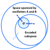
Figure 1: (color online). Leakage induced disentanglement of two noninteracting multilevel oscillators A and B coupled to a common reservoir. The outer, middle, and inner circles represent a set of subspaces spanned by combined oscillators A and B, the encoded subspace, and the entangled state $\sigma$ to be protected (i.e., protected subspace), respectively. The wavy arrows represent leakage.

We first consider two identical multilevel oscillators $A$ and $B$ undergoing longitudinal decay into a common zero-temperature bosonic reservoir. The resonant frequency $\omega_{0}$ and the dipolar coupling to the reservoir can be dynamically modulated by external fields with AC-Stark shifts $\lambda(t)$ and interaction strength $\varepsilon(t)$. The total Hamiltonian of the composite two-oscillator system plus the reservoir can be given by $\mathcal{H}=\mathcal{H}_{S}+\mathcal{H}_{R}+\mathcal{H}_{I},$ where (with $\hbar=1$)

$$\mathcal{H}_{S}=\mathbf{[}\omega_{0}+\lambda(t)\mathbf{]}\left(a_{A}^{{\dagger}}a_{A}+a_{B}^{{\dagger}}a_{B}\right),$$ (1)

$$\mathcal{H}_{R}=\sum_{l}\omega_{l}b_{l}^{\dagger}b_{l},$$ (2)

$$\mathcal{H}_{I}=\left(a_{A}^{{\dagger}}+a_{B}^{{\dagger}}\right)\sum_{l}\varepsilon(t)g_{l}b_{l}+\text{H.c.},$$ (3)

are Hamiltonians of the controlled system, the reservoir and their interaction DD ; book Qoptics . $a_{j}$ $(a_{j}^{{\dagger}})$ $(j=A,B)$ is the annihilation (creation) operator of the $j$th oscillator. $\omega_{l}$ and $a_{l}$ $(a_{l}^{\dagger})$ are, respectively, the frequency and the annihilation (creation) operator of the $l$th mode of the reservoir with the coupling $g_{l}$ to the oscillators. In the interaction picture, the Hamiltonian above is rewritten as

$$\mathcal{H}_{I}(t)=S(t)R(t)+S^{{\dagger}}(t)R^{{\dagger}}(t),$$ (4)

where $S(t)=\mathcal{M}(t)(a_{A}^{{\dagger}}+a_{B}^{{\dagger}})$, with $\mathcal{M}(t)=\varepsilon(t)e^{i\int_{0}^{t}d\xi\lambda(\xi)}$ the modulation function, and $R(t)=\sum_{l}g_{l}b_{l}e^{i(\omega_{0}-\omega_{l})t}.$ The dynamics of the density matrix $\rho(t)$ of the combined system-reservoir is governed by the von Neumann equation,

$$\frac{\partial}{\partial t}\rho(t)=-i[\mathcal{H}_{I}(t),\rho(t)]\equiv\mathcal{L}(t)\rho(t),$$ (5)

with $\mathcal{L}(t)$ the Liouville super-operator book open . It is convenient to check that $\left[\mathcal{H},\mathcal{N}\right]=0$ with the number operator $\mathcal{N}=a_{A}^{{\dagger}}a_{A}+a_{B}^{{\dagger}}a_{B}+\sum_{l}b_{l}^{\dagger}b_{l},$ implying $\mathcal{N}$ to be a conserved quantity. For multilevel oscillators, the system may suffer from disentanglement due to leakage from the protected subspace (or even from the encoded subspace) by the interaction with reservoir [shown in Fig. 1]. For example, we take levels $|0\rangle_{j}$ and $|1\rangle_{j}$ ($j=A,B$) to span the encoded subspace for qubits, and prepare the initial state of the system-reservoir in $(\alpha|11\rangle_{AB}+\beta|00\rangle_{AB})|0\rangle_{R}$, where $|0\rangle_{R}$ denotes the vacuum state of the reservoir. The system will be losing entanglement or even evolving outside the encoded subspace e.g., to the state $|20\rangle_{AB}|0\rangle_{R}$ or $|02\rangle_{AB}|0\rangle_{R}$.

Therefore, our primary aim is to construct a measure for the leakage induced disentanglement. In the present work, we assume the system to be initially prepared in an entangled state $\sigma$, which is to be protected. We need a measure to characterize how far the disentangled state tr${}_{R}\{\rho(t)\}$ is away form the protected state $\sigma$ [i.e., we consider the leakage out of the protected subspace, represented by the dark blue (black) wavy arrows in Fig. 1]. Such a measure can be $\mathcal{F}(\sigma,$tr${}_{R}\{\rho(t)\}),$ where

$$\mathcal{F}(x,y)=\left(\text{tr}\sqrt{\sqrt{x}y\sqrt{x}}\right)^{2},$$ (6)

is the fidelity to measure the distance between the density matrices $x$ and $y$ book QIP ; fidelity .

Our following aim is to seek a master equation for $\varrho(t)=\mathcal{F}(\sigma,$tr${}_{R}\{\rho(t)\})\sigma$, which can be accomplished by employing the Nakajima-Zwanzig projection operator technique book open . To eliminate the system-reservoir coherence, we first define the relevant part of $\rho(t)$ with a super-operator $\mathcal{P}$ note :

$$\mathcal{P}\rho(t)=\mathcal{F}(\sigma,tr_{R}\{\rho(t)\})\sigma\otimes\rho_{R},$$ (7)

where $\rho_{R}$ is supposed to be a stationary state of the reservoir in thermal equilibrium at zero temperature book Qoptics . Since the initial state of the system is prepared in the state $\sigma,$ i.e., $\mathcal{P}\rho(0)=\sigma\otimes\rho_{R},$ we may get a time-local homogeneous master equation of $\mathcal{P}\rho(t)$ as

$$\frac{\partial}{\partial t}\mathcal{P}\rho(t)=\mathcal{K}(t)\mathcal{P}\rho(t).$$ (8)

Here $\mathcal{K}(t)$ describes the time-convolutionless (TCL) generator book open . By restricting Eq. (8) to the second-order expansion of the system-reservoir coupling, i.e., $\mathcal{K}(t)=\int_{0}^{t}ds\mathcal{PL}(t)\mathcal{L}(s)\mathcal{P}$ (the TCL second-order approximation), we thus obtain the equation for $\varrho(t)$ as,

$$\frac{\partial\varrho(t)}{\partial t}=-\int_{0}^{t}ds\mathcal{F}(\sigma,\text{tr}_{R}\{[\mathcal{H}_{I}(t),[\mathcal{H}_{I}(s),\varrho(t)\otimes\rho_{R}]]\})\sigma.$$ (9)

Inserting $\varrho(t)=\mathcal{F}_{tcl}(t)\sigma$ into Eq. (9) with the notation $\mathcal{F}_{tcl}(t)=\mathcal{F}(\sigma,tr_{R}\{\rho(t)\}$, we obtain

$$\mathcal{F}_{tcl}(t)=\exp\left[-\int_{0}^{t}d\tau\int_{0}^{\tau}ds\mathbf{K}(s,\tau)\right],$$ (10)

where $\mathbf{K}(s,\tau)$ is the integral kernel with the form

$$\mathbf{K}(s,\tau)=\mathcal{F}[\sigma,G(s)\Theta(\tau,\tau-s)+\text{H.c.}],$$ (11)

$G(t)=$tr${}_{R}\{R(t)R^{{\dagger}}(0)\rho_{R}\}=\sum_{l}|g_{l}|^{2}e^{i(\omega_{0}-\omega_{l})t}=\int d\omega J(\omega)e^{i(\omega_{0}-\omega)t}$ is the reservoir correlation function with the sum over all transition matrix elements related to mode $\omega_{(l)}$. $J(\omega)$ is the spectral density, characterizing the reservoir spectrum density . We could model $J(\omega)$ by several typical spectrum functions, such as the Lorentzian or from sub-Ohmic to super-Ohmic forms density . In what follows, we consider, as an example, the oscillators interacting resonantly with a common reservoir with Lorentzian spectral distribution

$$J(\omega)=\frac{1}{2\pi}\frac{\gamma_{0}\Gamma^{2}}{(\omega_{0}-\omega)^{2}+\Gamma^{2}},$$ (12)

where $\gamma_{0}$ is the system decay rate in the Markovian limit and $\Gamma$ is the spectral width of the coupling book open , which has been widely employed in quantum optics book Qoptics . In addition, $\Theta(t_{1},t_{2})=[S(t_{1}),S^{{\dagger}}(t_{2})\sigma]=\mathcal{M}(t_{1})\mathcal{M}^{\ast}(t_{2})\bar{\sigma}$, with $\bar{\sigma}=[(a_{A}^{{\dagger}}+a_{B}^{{\dagger}}),(a_{A}+a_{B})\sigma]$ fully depending on the choice of the protected state $\sigma$. Therefore, we have

$$\mathbf{K}(s,\tau)=\frac{\gamma_{0}\Gamma}{2}e^{-\Gamma s}\mathcal{F}\left[\sigma,\mathcal{M}(\tau)\mathcal{M}^{\ast}(\tau-s)\bar{\sigma}+\text{H.c.}\right],$$ (13)

and particularly, if the protected state is a pure state $\sigma=|\chi\rangle\left\langle\chi\right|$, Eq. (13) reduces to

$$\mathbf{K}(s,\tau)=\eta\gamma_{0}\Gamma e^{-\Gamma s}\varepsilon(\tau)\varepsilon(\tau-s)\cos\left[\int_{\tau-s}^{\tau}d\xi\lambda(\xi)\right],$$ (14)

with $\eta=\left\langle\chi\right|\bar{\sigma}|\chi\rangle,$ where we have assumed $\varepsilon(t)$ to be real. Eq. (13) or Eq. (14) is one of the main results in this paper. We mention that Eq. (13) [or Eq. (14)] is universal for any entangled states to be protected. Let us go to some details below with two examples.

Example 1—We consider the oscillators as qubits, i.e., the protected state within $\{|0\rangle_{A},|1\rangle_{A}\}\otimes\{|0\rangle_{B},|1\rangle_{B}\}.$ Specifically, we assume the protected states to be in an extended Werner-like state (EWL) Wener

$$\sigma=r|\epsilon\rangle\left\langle\epsilon\right|+\frac{1-r}{4}\mathbf{1,}$$ (15)

where $r\in[0,1]$ and $|\epsilon\rangle=|\Phi\rangle=\alpha|11\rangle_{AB}+\beta|00\rangle_{AB}$ or $|\Psi\rangle=\alpha|10\rangle_{AB}+\beta|01\rangle_{AB}$. For the sake of conciseness, we consider two extreme cases: (i) For $r=1$, the EWL state reduces to the Bell-like pure state $\sigma=|\epsilon\rangle\left\langle\epsilon\right|$. We can get $\eta=2|\alpha|^{2}$ or $\eta=|\alpha+\beta|^{2}$ when $|\epsilon\rangle=|\Phi\rangle$ and $|\epsilon\rangle=|\Psi\rangle$, respectively. (ii) In the case of $r=0,$ the EWL state becomes totally mixed as $\bar{\sigma}=(|\theta\rangle_{AB}\left\langle 11\right|-|00\rangle_{AB}\left\langle 00\right|)/2$ with $|\theta\rangle=|11\rangle_{AB}+(|02\rangle_{AB}+|20\rangle_{AB})/\sqrt{2}$. The lengthy discussion for the case of $0<r<1$ will be left elsewhere.

Example 2—We consider the oscillators as qutrits, i.e., the protected state within the subspace spanned by $\{|0\rangle_{A},|1\rangle_{A},|2\rangle_{A}\}\otimes\{|0\rangle_{B},|1\rangle_{B},|2\rangle_{B}\}.$ We obtain $\eta=4|\alpha|^{2}+2|\beta|^{2}$ when the protected state is given by $\sigma=|\chi\rangle\left\langle\chi\right|$ with $|\chi\rangle=\alpha|22\rangle_{AB}+\beta|11\rangle_{AB}+$ $\gamma|00\rangle_{AB}.$ It is straightforward to extend the cases to other entangled states or higher dimensional systems, and the only difference will be the value of the coefficient $\mathcal{F}$ (or $\eta$).

It is necessary to check whether and to what extent the second-order TCL approximation can well characterize the dynamics of the two-oscillator system undergoing decay to a common reservoir. For convenience of description, we first ignore the external control, i.e., $\lambda(t)=0$ and $\varepsilon(t)=1$. In order to make a comparison between the exact and TCL solutions, we consider the state of oscillator-reservoir initially prepared in $|\Psi(0)\rangle=(\alpha|10\rangle_{AB}+\beta|01\rangle_{AB})\otimes|0\rangle_{R},$ i.e., at most one excitation of the reservoir at an arbitrary time: $|\Psi(t)\rangle=C_{10}(t)|10\rangle_{AB}|0\rangle_{R}+C_{01}(t)|01\rangle_{AB}|0\rangle_{R}+\sum_{l}C_{l}(t)|00\rangle_{AB}|1_{l}\rangle_{R}$, where $|1_{l}\rangle_{R}=b_{l}^{\dagger}|0\rangle_{R}$ is the reservoir state with one excitation in the mode $l$. Only in this case, is there an exact analytical solution to the fidelity by directly solving the Schrödinger equation $i\frac{\partial|\Psi(t)\rangle}{\partial t}=\mathcal{H}|\Psi(t)\rangle$ one exciton . For simplicity, considering the initial state of the oscillators in $|\Psi\rangle=(|10\rangle_{AB}+|01\rangle_{AB})/\sqrt{2},$ one immediately has

$$\mathcal{F}_{ext}^{|\Psi\rangle}(t)=\frac{1}{2}|C_{10}(t)+C_{01}(t)|^{2},$$ (16)

where $C_{10}(t)=C_{01}(t)=e^{-\Gamma t/2}\left[\cosh(\kappa t/2)+(\Gamma/\kappa)\sinh(\kappa t/2)\right]/\sqrt{2}$ with $\kappa=\sqrt{\Gamma(\Gamma-4\gamma_{0})}$. The corresponding approximate solution reduces to

$$\mathcal{F}_{tcl}^{|\Psi\rangle}(t)=\exp\left[-2\gamma_{0}\left(t+\frac{e^{-\Gamma t}-1}{\Gamma}\right)\right].$$ (17)

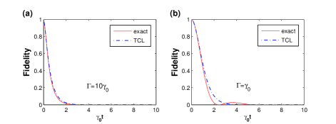
Figure 2: (color online). The fidelity for the initial state $(|10\rangle_{AB}+|01\rangle_{AB})/\sqrt{2}$ as a function of $\gamma_{0}t$ with (a) $\Gamma=10\gamma_{0}$ and (b) $\Gamma=\gamma_{0}.$ The solid (red) lines and dot-dashed (blue) lines represent the exact analytical solution and TCL approximate solution, respectively.

We have plotted Fig. 2 for the validity of TCL approximation, where the TCL approximation is valid in describing the true dynamics of the system in the weak coupling regime, i.e., $\Gamma\gg\gamma_{0}$ [See Fig. 2(a)]. But if $\Gamma$ is comparable or smaller than $\gamma_{0}$, the agreement between the exact analytical and the approximate solutions occurs only for the short-time behavior, e.g., $t\leq\Gamma^{-1}$, as shown in Fig. 2(b).

In what follows, as an illustration, we will concentrate on the entanglement preservation by some non-ideal pulses by means of Eq. (13) or (14) within the short-time regime. Unlike idealized BB control, which requires unrealistic arbitrarily strong and instantaneous control pulses, we are going to employ non-ideal impulse phase modulation with $\varepsilon(t)=1$ and a periodic rectangular interaction pulse nonideal control :

$$\lambda(t)=\begin{cases}\Lambda/\Delta,&for\text{ }nT-\Delta<t<nT,\\ 0,&otherwise,\end{cases}$$ (18)

where $T$, $\Delta$ and $\Lambda=\int_{nT-\Delta}^{nT}\lambda(t)dt$ are the period, width and interaction intensity of pulses, which are also the three main control parameters in the scheme. By numerical treatment, we seek, using the non-ideal quantum control, the solution to the equation $\delta\mathcal{F}_{tcl}(t;T,\Delta,\Lambda)=0$ with respect to all control parameters at time $t$ nonideal control . As an example, we employ the pure entangled state to be protected, and the extension to a general mixed entangled state is straightforward. We assume $\eta=1$ [corresponding to, for example, entangled qubit state $(|11\rangle_{AB}+|00\rangle_{AB})/\sqrt{2}$ or qutrit state $(|22\rangle_{AB}+|11\rangle_{AB}+$ $2|00\rangle_{AB})/\sqrt{6}$] and consider the case with $\Gamma=\gamma_{0}$, which yields the fidelity to be $\mathcal{F}_{tcl}(t)=\exp\left[-\int_{0}^{t}d\tau\int_{0}^{\tau}ds\gamma_{0}^{2}e^{-\gamma_{0}s}\cos(\int_{\tau-s}^{\tau}d\xi\lambda(\xi))\right]$. This makes it possible to study the entanglement preservation on the timescale of $\gamma_{0}^{-1}$.

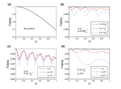
Figure 3: (color online). The fidelity for an initial pure state with $\eta=1$ [e.g., for $(|11\rangle_{AB}+|00\rangle_{AB})/\sqrt{2}$ and $(|22\rangle_{AB}+|11\rangle_{AB}+$ $2|00\rangle_{AB})/\sqrt{6}$] as a function of $\gamma_{0}t$ in non-Markovian regime $\Gamma=\gamma_{0}$, where (a) no external field control is performed; (b) $\sim$(d) non-ideal impulsive phase modulation of the coupling with fixed $\Lambda$, $\Delta;\Lambda$, $T;$ and $T$, $\Delta$, respectively. The solid (black) lines represent the approximate solutions of $\delta\mathcal{F}_{tcl}(t;T,\Delta,\Lambda)=0$ with respect to variable control parameters $T$, $\Delta$, and $\Lambda$ at an arbitrary time $t$, respectively.

To have a comparison, the fidelities of two oscillators undergoing decay with and without external field control are depicted in Fig. 3. It is clear that the fidelity drops fast within the timescale of $\gamma_{0}^{-1}$ in the absence of the pulse control. In contrast, in the presence of pulse control, despite the pulses with difference in pulse period $T$, pulse width $\Delta$ and interaction intensity $\Lambda$, the fidelity would be more or less maintained. We have found that the pulse control works better with $T$ decreasing, provided the fixed $\Lambda$ and $\Delta$. As shown in Fig. 3(b), when $\Lambda=\pi$, $T=\Delta=0.05\gamma_{0}^{-1}$, the fidelity nearly remains to be 1. This may be understood as that the control in this case equals to an addition of a constant frequency $\Lambda/T$ to the oscillator frequency $\omega_{0}$, and thereby $\Theta$ is oscillating fast, i.e., the minimum overlap between the reservoir correlation spectral and the modulation spectral. So the fidelity keeps nearly 1. But for the fixed values of $\Lambda=\pi$ and $T=0.1\gamma_{0}^{-1}$, as plotted in Fig. 3(c), the control seems weakly dependent on the pulse width. Fig. 3(d) demonstrates the dependence of the control effect on the interaction intensity $\Lambda$: the increase of $\Lambda$ leads to a better control.

The above analysis can be extended to oscillators under other modulations with realistic parameters. In addition, in future work we will explore the details of the leakage, which would be helpful for deeply understanding the physical mechanism behind the dynamics of multilevel systems as well as for seeking efficient ways to prevent disentanglement of multilevel systems. Practically, it would be of great interest to test our strategy experimentally by real physical systems, e.g., using two entangled atoms confined in optical microcavities QED .

In conclusion, based on the Nakajima-Zwanzig projection operator technique, we have characterized by fidelity the disentanglement of two multilevel oscillators coupled to a common reservoir. We have developed a universal expression which well fits the exact solution in weak coupling regime and strong coupling regime within a short-time period. We have also investigated the behavior of the oscillators under non-ideal pulse control, which shows that entanglement could be well protected with high fidelity. We expect that our strategy would be useful for better understanding dissipative dynamics of the multilevel open quantum systems and for better operations in quantum information processing.

This work is supported by the National Natural Science Foundation of China under Grant No. 10774163.

References

- (1) R. Horodecki et al., Rev. Mod. Phys. 81, 865 (2009).
- (2) M. A. Nielsen and I. L. Chuang, Quantum Computation and Quantum Information (Cambridge University Press, Cambridge, England, 2000).
- (3) H.-P. Breuer and F. Petruccione, The Theory of Open Quantum Systems (Oxford University Press, Oxford, 2007).
- (4) T. Yu and J. H. Eberly, Science 323, 598 (2009).
- (5) I. Sainz and G. Björk, Phys. Rev. A 77, 052307 (2008).
- (6) J. Kempe et al., Phys. Rev. A 63, 042307 (2001).
- (7) B. Bellomo, R. L. Franco and G. Compagno, Phys. Rev. Lett. 99, 160502 (2007); B. Bellomo et al., Phys. Rev. A 78, 060302(R) (2008).
- (8) S. Das and G. S. Agarwal, e-print arXiv:1004.0564.
- (9) A. R. R. Carvalho and J. J. Hope, Phys. Rev. A 76, 010301(R) (2007); A. R. R. Carvalho et al., ibid. 78, 012334 (2008).
- (10) See, e.g., G. Gordon and G. Kurizki, Phys. Rev. Lett. 97, 110503 (2006); G. Gordon, J. Phys. B 42, 223001 (2009), and references therein.
- (11) S. Maniscalco et al., Phys. Rev. Lett. 100, 090503 (2008).
- (12) L.-A. Wu, G. Kurizki, and P. Brumer, Phys. Rev. Lett. 102, 080405 (2009).
- (13) L. Viola and S. Lloyd, Phys. Rev. A 58, 2733 (1998).
- (14) M. O. Scully and M. S. Zubairy, Quantum Optics (Cambridge University Press, New York, 1997); D. F. Walls and G. J. Milburn, Quantum Optics (Springer-Verlag, Berlin, 2008).
- (15) R. Jozsa, J. Mod. Opt. 41, 2315 (1994).
- (16) Our evaluation of entanglement preservation is not restricted to the use of fidelity, but for any measure of the distance between two density matrices, e.g., trace distance book QIP . However, the definition here provides an intuitive justification: When the protected state is a pure state , we have . So can be taken as a projection operator to project a leaked state to the protected state, which is in agreement with the statement in Ref. nonideal control .
- (17) A. J. Leggett et al., Rev. Mod. Phys. 59, 1 (1987).
- (18) R. F. Werner, Phys. Rev. A 40, 4277 (1989).
- (19) B. M. Garraway, Phys. Rev. A 55, 2290 (1997).
- (20) K. J. Vahala, Nature (London) 424, 839 (2003).