Quest for the control on the second order derivatives: topology optimization with functional includes the state’s curvature

Abstract.

Many physical phenomena, governed by partial differential equations (PDEs), are second order in nature. This makes sense to pose the control on the second order derivatives of the field solution, in addition to zero and first order ones, to consistently control the underlaying process. However, this type of control is nontrivial and to the best of our knowledge there is nigher a theoretic nor a numeric work in this regard. The present work goals to do the first quest in this regard, examining a problem of this type using a numerical simulation.

A distributed parameter identification problem includes the control on the diffusion coefficient of the Poisson equation and a functional includes the state’s curvature is considered. A heuristic regularization tool is introduced to manage codimension-one singularities during the functional analysis. Based on the duality principles, the approximate necessary optimality conditions is found. The system of optimality conditions is solved using a globalized projected gradient method. Numerical results, in two- and three-dimensions, implied the possibility of posing control on the second order derivatives and success of the presented numerical method.

Keywords. adjoint sensitivity, distributed parameter identification, pointwise Hessian constraint, regularization singular integral, second order control.

1. Introduction

Many problems in engineering sciences and physics are modeled by partial differential equations (PDEs). The numerical solution of PDEs provides useful information for design engineers to predict the behaviors of corresponding systems. In the highly competitive world of today, it is no longer sufficient to design a system that performs the required task satisfactorily, but it is desired to find the optimal conditions. The PDE-constrained optimization (cf. [14, 4]) is an effective way to approach this goal.

In the context of PDE-constrained optimal control it is common to pose either pointwise or global control on the state solution and/or state’s derivatives. Most of works in this regard are focused to apply control on the the zero and/or first order derivatives of filed solution.

However, most of the physical phenomena are spatial second order in nature. This means that the behavior of a point is a function of its neighborhood. This make sense to pose control on the second order derivatives of the state solution, in addition to the zero and/or first order derivatives. Moreover, in some cases we may not have sufficient information about the desired conditions in terms of the zero and/or first order information. Lets to give an instance, to make the mentioned problem more clear. In heat transfer problems, hot-centers (the locus of heat flux concentration) are a subset of temperature field critical points, i.e., where the temperature gradient approaches to zero. Now assume we want to control the position of hot centers. It is clear that to pose the control on the state’s gradient does not make a physically consistent design problem, because, the cold-centers and saddle points are also included within the set of mentioned critical points. An effective way to consistently contrast between these three types of points, is to consider the second order information too, i.e., to include the Hessian of the state solution. It is worth mentioning that, some of the currently used design problems could be enriched/regularized by including the second order information in their formulation.

However, to pose the control on the second order information is not an easy task. To the best of our knowledge there is neither a theoretic nor a numeric work in this regard. Since theoretical study on this topic is not easy using available functional analysis tools, we shall perform a numerical quest on this topic here. To be more specific, we consider a topology optimization problem (cf. [4]) in this study. Our problem includes the minimization of an integral functional includes the state’s first and second order derivatives where the sate is governed by a Poisson equation. Moreover the diffusion coefficient of the Poisson equation is the control parameter in this study. In fact we deal with a PDE-constrained distributed parameter identification problem in this study.

2. Problem statement

Consider a simply connected domain $Q\subset\mathbb{R}^{d}$ ($d=$ 2 or 3), with sufficiently regular boundary $\Sigma=\partial Q$, where the optimization problem will take place. Consider the following design problem in steady-state heat (or electrical) conduction: given two isotropic conducting materials, with thermal conductivities $\alpha$ and $\beta$, $0<k_{\beta}<k_{\alpha}$. Suppose that at each spatial point $\textbf{x}\in Q$ the conductivity is given in terms of the $\alpha-$phase characteristic function $\chi=\chi(\textbf{x})$, where $\chi\in\{0,1\}$, as follows:

$$k(\chi)=\chi k_{\alpha}+(1-\chi)k_{\beta}$$ (2.1)

where $k_{\alpha}$ and $k_{\beta}$ denote the thermal (or electrical) conductivity of phases $\alpha$ and $\beta$ respectively. In fact, $\chi(\textbf{x})$ plays the role control or design parameter here. The goal is to find $\chi(\textbf{x})$ configuration which solve the following design problem:

$$\mathtt{(P)}:=\ \ \arg\min_{\chi\in\Upsilon}F(\chi)=\int_{\mathcal{D}}f(\chi,\nabla u,\nabla\nabla u)\ d\Omega$$

subject to:

$$\nabla\cdot\big{(}k(\chi)\nabla u\big{)}=g(\mathbf{x})\ \ \mathtt{in}\ Q,\ \ u=u_{0}\ \ \textrm{on}\ \Sigma$$ (2.2)

where $\mathcal{D}\subseteq\Omega$ denotes the support domain of the integral functional, $d\Omega$ denotes the volume measure induced in $Q$, $u\in X_{u}(Q)$ is the state function, $\nabla u$ is the state gradient, $\nabla\nabla u$ denotes the local Hessian matrix of the state function, i.e., $\nabla\nabla u=[u_{ij}]_{d\times d}$, $i,j\in\{x,y\}$ ($u_{ab}=\frac{\partial^{2}u}{\partial a\partial b}$), $g\in X_{g}(Q)$ is a given source function, $u_{0}(\textbf{x})\in X_{u}(Q)$ denotes the Dirichlet boundary condition and $\Upsilon$ denotes the admissible design space which is defined as follows

$$\Upsilon:=\big{\{}\chi\in X_{\chi}(Q)\ \big{|}\quad\ R_{L}|Q|\leq\int_{Q}\chi d\Omega\leq R_{U}|Q|,\quad\chi\in\{0.1\}\ \big{\}}$$ (2.3)

where $0<R_{L}\leq R_{U}<1$ are given lower and upper bounds on $\alpha$-phase material resource respectively, and $|\Omega|$ denotes the measure of $\Omega$ (volume for $d=3$ and area for $d=2$). In above formulae $X_{u}$, $X_{g}$ and $X_{\chi}$ denotes some appropriate Banach spaces. Since our goal in this study is not to do a rigorous mathematical analysis, we simply assume that these function spaces possess sufficiently regularity required by our analysis. It is well known that optimal design problems like $\mathtt{(P)}$, are ill-posed and do not admit an optimal solution in class of characteristic functions (cf. [8]). The relaxation form of these problem is usually achieved extending the design domain $\Xi$ to the convex and continuous space $\Xi$ which is defined as follows,

$$\Xi=\big{\{}w\in X_{w}(Q)\ \big{|}\quad\ R_{L}|Q|\leq\int_{\Omega}w\ d\textbf{x}\leq R_{U}|Q|,\quad 0\leq w\leq 1\big{\}}$$ (2.4)

where $X_{w}$ is a sufficiently regular Banach space. In fact in the relaxed design problem the material conductivity could varies gradually between phases $\alpha$ and $\beta$ and we have somehow a functionally graded material. The SIMP approach [4] is employed in this study to achieve a near 0-1 topology. In this method the conductivity function (2.1) is replaced by the following function:

$$k(w)=w^{q}(k_{\alpha}-k_{\beta})+k_{\beta}$$ (2.5)

where $q\geq 1$ is a penalization factor which is commonly called as the SIMP power.

In the present study, the function $f$ in $\mathtt{(P)}$ is assumed to have the following form:

$$f:=aw^{b}(\kappa-\kappa_{0})^{c},$$

where $a,b,c\in\mathbb{R}$, $b,c\geq 1$ are some given constants, $\kappa$ is the local mean curvature of state iso-contours, i.e., $\kappa=\nabla\cdot(\nabla u/|\nabla u|)$. It is clear that $\kappa$ is a nonlinear function of both the first and second order derivatives of $u$ (cf. [15]). Therefore, this type of functional it is a fairly good choice for the purpose of this study. Besides it has a clear physical interpretation and has certain applications in practical design problems. For example, a negative curvature with large absolute value is signature of thermal centers in the heat transfer problems (cf. [18]).

3. Regularization of the curvature singularities

Assume $u_{0}$ is a constant function on $\Gamma$, then according to the maximum principles, there is at least a point $\mathbf{x}_{0}\in\Omega$ such that $|\nabla u|=0$). To avoid the curvature singularity in this regard, we simply replace $|\nabla u|$ by $|\nabla u|_{\varepsilon}:=\sqrt{\varepsilon^{2}+|\nabla u|^{2}}$ in the definition of mean curvature. Therefore the regularized mean curvature is defined as follows: $\kappa_{\varepsilon}=\nabla\cdot(\nabla u/|\nabla u|_{\varepsilon})$, where the small number $\varepsilon\in\mathbb{R}^{+}$ is the curvature regularization parameter. For the purpose of convenience we simply use $\kappa$ instead of $\kappa_{\varepsilon}$ henceforth. In practice we use a sufficiently small value ($10^{-20}$ in this study) instead of $\varepsilon$ without any outer iteration on $\varepsilon$ to recover the original problem.

Consider the discretized version of the optimal design problem with the minimum grid size $h$. According to [15], the maximum absolute value of the curvature which can be resolved by such a grid resolution is equal to $\frac{1}{h}$. Therefore, if the computed value of $\kappa$ locates outside of $-\frac{1}{h}\leq\kappa\leq\frac{1}{h}$, we merely replace that value with either $-\frac{1}{h}$ or $\frac{1}{h}$ depending on the sign of curvature.

4. A Local analysis near a shallow gradient regions

Suppose that $u$ is $C^{2}$ near a generic spatial stationary point $\textbf{x}_{0}$, i.e., $|\nabla u|=0$ and $\nabla\nabla u$ is nonsingular there. Consider d-dimensional closed ball $\mathcal{B}_{r}\subset Q$ with radius $r\in\mathbb{R}^{+}$ centered at $\mathbf{x}_{0}$. We would like to study the behavior of the objective functional in $(\mathtt{P})$ restricted to ball $\mathcal{B}_{r}$. In this regard we can restrict ours to case $\kappa_{0}=0$ i.e., to study the behavior of the following functional:

$$F|_{\mathcal{B}_{r}}:=\int_{\mathcal{B}_{r}}aw^{b}\kappa^{c}\ d\Omega$$ (4.1)

Since $\kappa$ is invariant under an Euclidean transformation, we assume $\mathbf{x}_{0}=\mathbf{0}$. Consider an approximation of $u$ in the neighborhood of $\mathbf{x}_{0}$ by the Taylor expansion up to the second order derivatives (recall that $|\nabla u(\mathbf{x}_{0})|=0$):

$$u(\textbf{x})\approx u(\mathbf{x}_{0})+\frac{1}{2}\ \textbf{x}^{T}\cdot\nabla\nabla u(\mathbf{x}_{0})\cdot\textbf{x}$$ (4.2)

Since $\kappa$ is rotationally invariant, we can assume that

$$\nabla\nabla u(\mathbf{x}_{0})=\texttt{diag}(\lambda_{0}(\mathbf{x}_{0}),\cdots,\lambda_{d}(\mathbf{x}_{0}))$$ (4.3)

where $\lambda_{i}(\mathbf{x}_{0})$ denotes the $i$-th eigenvalue of $\nabla\nabla u(\mathbf{x})$ at $\mathbf{x}=\mathbf{x}_{0}$. Therefore, by 4.2 we have

$$u(\textbf{x})\approx u(\mathbf{x}_{0})+\frac{1}{2}\ \sum_{i=1}^{d}\lambda_{i}(\mathbf{x}_{0})x_{i}^{2}$$ (4.4)

The local structure of the solution in the vicinity of $\textbf{x}_{0}$ is a function of relative values of $\lambda_{i}(\mathbf{x}_{0})$. There are four generic types of local structures in this regard: sheet-like, tube-like, blob-like, double-cone-like local structures. Among these local features, the blob (ellipsoidal) and double-cone (hyperbolic) types have the maximum mean curvature concentration. For the ease of analysis, we restrict ours to the blob-like local structures (when $\lambda_{1}\approx\cdots\approx\lambda_{d}$). Assume $\lambda_{1}\approx\cdots\approx\lambda_{d}=\lambda$, i.e., a spherical local structure, using (4.4) and straightforward computations, we have:

$$\kappa=\frac{d-1}{\sqrt{\sum_{i=0}^{d}x_{i}^{2}}}$$ (4.5)

substitution of 4.5 in 4.1 results:

$$F|_{\mathcal{B}_{r}}=\int_{\mathcal{B}_{r}}aw^{b}\bigg{(}\frac{d-1}{\sqrt{\sum_{i=0}^{d}x_{i}^{2}}}\bigg{)}^{c}\ d\Omega$$ (4.6)

Considering the symmetric structure of the blob-like structure and using the spherical coordinate results:

$$F|_{\mathcal{B}_{r}}=\int_{0}^{r}aw^{b}\bigg{(}\frac{d-1}{r}\bigg{)}^{c}\ \pi(2r)^{d-1}dr=\zeta\int_{0}^{r}r^{d-c-1}\ dr$$ (4.7)

where constant $\zeta$ is equal to $2^{(d-1)}(d-1)^{c}\pi aw^{b}$. Considering 4.7, integral functional 4.1 is well-defined in the vicinity of a regular shallow gradient point if $c\leq d-1$. It turns out that we are not free to select the power of the curvature term in our integral functional. For instance, assume we are interested to solve a topology optimization problems subject to pointwise constraints on mean curvature. According to above analysis, in the case of two dimensions, we can not use a quadratic (or higher order) penalty function (cf. [5, ch. 3]) to manage local constraints (it is worth mentioning that using quadratic penalty functions is very common to manage such problems. In the other word we have to use exact penalty functions (cf. [5, ch. 4]) in these cases.

5. Regularization of singular integrals

To derive the first order necessary optimality conditions we have to deal with some singular integrals to continue the analysis. The good of this section is to introduce some (heuristic) regularization tools to manage such cases. Let $f(\textbf{x}):\mathbb{R}^{d}\rightarrow\mathbb{R}$ be a real-valued function defined on the codimension-one $C^{2}$ manifold $\mathcal{M}\subset\mathbb{R}^{d}$ which is embedded within domain $Q$. We are interested to compute the following singular integral:

$$I:=\int_{\mathcal{M}}f(\textbf{x})\ d\Gamma=\int_{Q}f(\textbf{x})\ \delta(\mathcal{M})\ d\Omega$$ (5.1)

where $d\Gamma$ denotes the surface measure induced on $\mathcal{M}$, $\delta(\mathcal{M})$ denotes the delta-distribution concentrated on $\mathcal{M}$. Consider $b_{\mathcal{M}}\in C^{1}(\Omega)$ as the Euclidean signed distance function with respect to manifold $\mathcal{M}$. Assume $(\cdot)^{ext}_{\sigma}$ denotes the smooth extension (along the normal direction) of scaler field $(\cdot)$ defined on $\mathcal{M}$ into $\mathcal{N}(\mathcal{M},\sigma)$, where $\mathcal{N}(\mathcal{M},\sigma)$ denotes $\pm\sigma$-distance neighborhood of $\mathcal{M}$. Moreover assume that the manifold forms the boundaries of $\mathcal{N}(\mathcal{M},\sigma)$ is non-degenerate (there is no self-crossing). Assume that $\mathcal{N}(\mathcal{M},\sigma)$ is spanned by $s\lambda$-system such that $s$ coincides to the iso-contours of the distance function $b_{\mathcal{M}}$ and $\lambda$ coincides to normals on the $b_{\mathcal{M}}$-constant surfaces. Therefore, $ds$ is a $(d-1)$-dimensional (area) metric and $d\lambda$ is a one-dimensional metric. It is obvious that $s\lambda$-system consistently spans $\mathcal{N}(\mathcal{M},\sigma)$, if iso-contours of $b_{\mathcal{M}}$ do not cross each other (which is followed by our assumption). Therefore we can use $s\lambda$-system together with its corresponding d-dimensional volume element, $dsd\lambda$, to compute $d$-dimensional volume integrals. Applying $s\lambda$-system to integral (5.1) results:

$$I_{\sigma}=\int_{\lambda=-\sigma}^{\lambda=+\sigma}\rho_{\sigma}(\lambda)\int_{\mathcal{M}_{b}:\ b_{\mathcal{M}}=\lambda}f^{ext}_{\sigma}(\textbf{x})\ ds\ d\lambda$$ (5.2)

where $\lim_{\sigma\rightarrow 0}I_{\sigma}=I$, the manifold $\mathcal{M}_{b}\subset\mathcal{N}(\mathcal{M},\sigma)$ coincides to an $s$-surface which is located at distance $b$ from $\mathcal{M}$, and the weighting function $\rho_{\sigma}\in C^{\infty}(\mathbb{R})$ is chosen such that the intensity (measure) of $f(\textbf{x})$ be preserved, i.e.,

$$\int_{\lambda=-\sigma}^{\lambda=+\sigma}\rho_{\sigma}(\lambda)\ d\lambda=1$$ (5.3)

the other requirements of function $\rho_{\sigma}$ are: $\rho_{\sigma}(x)\neq 0$ for $x\in(-\sigma,+\sigma)$, $\rho_{\sigma}(x)=0$ for $x\notin(-\sigma,+\sigma)$. In fact, $\rho_{\sigma}$ makes a converging sequence to the classic delta function, $\delta$, in the sense that: $\lim_{\sigma\rightarrow 0}\rho_{\sigma}(x)=\delta(x)$ (cf. [6]). in the present study, the following normalized Gaussian distribution is used as $\rho_{\sigma}$ function:

$$\rho_{\sigma}(\lambda)=\newline \left\{\begin{array}[]{lll}\rho_{\sigma}^{0}\ \sigma^{-d}\ \exp\big{(}\frac{\sigma^{2}}{|\lambda|^{2}-\sigma^{2}}\big{)},&\texttt{if}&|\lambda|<\sigma\\ 0,&\texttt{if}&|\lambda|\geq\sigma\end{array}\right.$$ (5.4)

where $\rho_{\sigma}^{0}$ is determined bases on constraint (5.3). Note that $\rho_{\sigma}$ plays also the role of a regularization kernel in our formulation (cf. [20, 7]). More precisely, for every point $\textbf{x}_{0}\in\mathcal{M}$, $\rho_{\sigma}$ does convolution of $f(\textbf{x}_{0})$ along the line segment $(-\sigma,+\sigma)$ which is normal to $\mathcal{M}$ and passes from $\textbf{x}_{0}$. Therefore, if the extension of $f$ to neighborhood of the desired manifold be not smooth, e.g., there are some equi-distanced points from the manifold surfaces, our method performs well.

Now, lets to back from $s\lambda$-coordinate to our original Cartesian coordinate. The coarea formula [10] is used for this purpose. Assume that the change of variable is global in $\Omega$, the coarea formula can be expressed as:

$$\int_{\Omega}|\nabla b_{\mathcal{M}}|\ d\Omega=\int\ ds\ d\lambda$$ (5.5)

i.e., $|\nabla b_{\mathcal{M}}|\ d\Omega=ds\ d\lambda$ (cf.: [9, ch. 3]). Applying (5.5) to (5.2) results:

$$I_{\sigma}=\int_{\mathcal{N}(\mathcal{M},\sigma)}\rho_{\sigma}(b_{\mathcal{M}}(\textbf{x}))\ f^{ext}_{\sigma}(\textbf{x})\ |\nabla b_{\mathcal{M}}|\ d\Omega$$ (5.6)

since $\rho_{\sigma}=0$ for $\mathbf{x}\in\Omega\setminus\mathcal{N}(\mathcal{M},\sigma)$,

$$I_{\sigma}=\int_{\Omega}\rho_{\sigma}(b_{\mathcal{M}}(\textbf{x}))\ f^{ext}_{\sigma}(\textbf{x})\ |\nabla b_{\mathcal{M}}|\ d\Omega$$ (5.7)

it is worth noticing that a formula similar to (5.7) is derived heuristically (not rigorously) in [15, ch. 1].

The Euclidean signed distance function $b_{\mathcal{M}}$ can be efficiently computed solving the following eikonal equation [16, 15]:

$$|\nabla b_{\mathcal{M}}|=1\ \ \mathtt{in}\ \ Q,\quad b_{\mathcal{M}}=0\ \ \mathtt{on}\ \ \mathcal{M}$$ (5.8)

this equation can be solved efficiently using either the fast marching method [16]. Notice that the solution of (5.8) is a member of $BV(Q)$, i.e., it is not essentially sufficiently smooth. However, due to the application of the regularization kernel $\rho_{\sigma}$ in our formulation, we are not concerned about the smoothness of $b_{\mathcal{M}}$. We also need to extend function $f$ defined on $\mathcal{M}$ along the normal direction into $\mathcal{N}(\mathcal{M},\sigma)$. The following PDE is suggested in [1] to do this job:

$$f^{ext}\cdot\nabla b_{\mathcal{M}}=0\ \ \mathtt{in}\ \ Q,\ \ f^{ext}=f\ \ \mathtt{on}\ \ \mathcal{M}$$ (5.9)

where $f^{ext}$ denotes the extension of $f$ inside $\mathcal{N}(\mathcal{M},\sigma)$. In [1], an efficient fast marching method is suggested to compute $b_{\mathcal{M}}$ and $f^{ext}$ simultaneously. The implementation of this method will be used in this study.

For the convenience in notation, the following notation is used in this study, everywhere required:

$$\int_{\mathcal{M}}(\cdot)\ d\Gamma\equiv\int_{\mathcal{N}(\mathcal{M},\sigma)}\langle\langle\ (\cdot)\ \rangle\rangle\ d\Omega$$ (5.10)

Let $a(\textbf{x})$ and $b(\textbf{x}):\mathbb{R}^{d}\rightarrow\mathbb{R}$ and $\textbf{c}(\textbf{x})$ and $\textbf{d}(\textbf{x}):\mathbb{R}^{d}\rightarrow\mathbb{R}^{d}$ be functions defined on co-dimension one manifold $\mathcal{M}$. To do our sensitivity analysis, we need the following properties for operator $\big{<}\big{<}(\cdot)\big{>}\big{>}$ (note that these relations are not exactly hold however we are hopeful, without proof, to validity of them in the sense of approximation):

$$\int_{(\cdot)}\langle\langle\ a\ b\ \rangle\rangle\ d\Omega \approx \int_{(\cdot)}\langle\langle\ a\ \rangle\rangle\ b\ d\Omega$$ (5.11)

$$\int_{(\cdot)}\langle\langle\ \textbf{c}\cdot\textbf{d}\ \rangle\rangle\ d\Omega \approx \int_{(\cdot)}\langle\langle\ \textbf{c}\ \rangle\rangle\cdot\textbf{d}\ d\Omega$$ (5.12)

6. The first order necessary optimality conditions

There are several methods to solve a distributed parameter identification problem. Due to large number of control parameters, a gradient based method is adapted in this study (cf. [3]). Lets to define the meaning of differentiability on function spaces. There exist several differentiability notions in mathematical programming literature. The notion of Gâteaux derivative is applied here.

Definition 6.1.

(Gâteaux derivative, cf. [3]) Consider Banach spaces $Y$ and $W$ and $U$ as open subset of $Y$. A function $f:U\rightarrow W$ is called to be Gâteaux differentiable at $u\in U$ if for every test function $v\in Y$ the following limit exist:

$$f^{\prime}(u):=\lim_{\zeta\rightarrow 0}\frac{f(u+\zeta v)-f(u)}{\zeta}$$

In this case we show the Gâteaux derivative symbolically by $f^{\prime}(u)$. If $Y$ is a Hilbert space, which is assumed in this study, then $f^{\prime}(u)$ lives on the dual space of $Y$. Therefore using the Riesz representation theorem, there is a unique $e\in Y$ such that $\langle e,v\rangle=f^{\prime}(u)$, where $\langle\cdot,\cdot\rangle$ denotes the inner product on $Y$. In this case, without confusion, it is common to call $e$ as the Gâteaux derivative. We use notation $df(u)$ in this case, i.e., $df(u)=e$. It is easy to verify that under some mild conditions (which usually hold in practice) most of properties for classical derivatives have equivalent extension to Gâteaux derivative. In the case of multi-variable functional, the partial Gâteaux derivative are denoted by $f^{\prime}_{(\cdot)}$, $\partial_{(\cdot)}f(\cdots)$ symbols in this study. For the purpose of convenience the Gâteaux derivative is called as the directional derivative in this study, henceforth. Without confusion, the notation $\langle\cdot,\cdot\rangle_{Q}:=\int_{Q}(\cdot)(\cdot)\ d\Omega$ also used to denote the duality pairing on function spaces in this study.

Consider an arbitrary function $p\in X_{p}(Q)$, where $X_{p}$ is a sufficiently regular Banach space. Lets to introduce the following lagrangian augmenting the inner product of $p$ and the Poisson equation to the objective functional in problem $\mathtt{(P)}$:

$$\mathcal{L}(w,u,p):=F(w,u)+\big{\langle}\nabla\cdot(k\nabla u)-g,\ p\big{\rangle}_{Q}+\big{\langle}u-u_{0},\ p\big{\rangle}_{\Sigma}$$

The set of points satisfy the first order necessary optimality conditions of problem $\mathtt{(P)}$, denoted by $\mathcal{O}$ can be expressed as follows (cf. [3]):

$$\mathcal{O}:=\left\{(w,u,p)\in\big{(}\Xi\times X_{u}(Q)\times X_{p}(Q)\big{)}\ \Bigg{|}\begin{array}[]{r}\partial_{w}\mathcal{L}(w,u,p)=0\ \ \texttt{in}\ Q\ \ (\mathtt{C.1})\\ \partial_{u}\mathcal{L}(w,u,p)=0\ \ \texttt{in}\ Q\ \ (\mathtt{C.2})\\ \partial_{p}\mathcal{L}(w,u,p)=0\ \ \texttt{in}\ Q\ \ (\mathtt{C.3})\end{array}\right\}.$$

where $\partial_{w}\mathcal{L}$, $\partial_{u}\mathcal{L}$ and $\partial_{p}\mathcal{L}$ denote respectively the partial directional derivatives of $\mathcal{L}$ with respect to $w$, $u$ and $p$ along arbitrary test directions $\delta w\in X_{w}(Q)$, $\delta u\in X_{u}(Q)$ and $\delta p\in X_{p}(Q)$ respectively. In fact, $\mathcal{O}$ includes constrained stationary points of augmented lagrangian $\mathcal{L}$. Regarding to $\partial_{w}\mathcal{L}$ in condition $(\mathtt{C.1})$ of set $\mathcal{O}$ we have,

$$\big{\langle}\partial_{w}\mathcal{L},\delta w\big{\rangle}_{Q} =\big{\langle}\partial_{w}f,\ \delta w\big{\rangle}_{\mathcal{D}}+\big{\langle}p\nabla\cdot(\partial_{w}k\nabla u),\ \delta w\big{\rangle}_{Q}:=I_{1}+I_{2}$$ (6.1)

where $\partial_{w}f=abw^{(b-1)}(\kappa-\kappa_{0})^{c}$ and $\partial_{w}k=qw^{(q-1)}(k_{\alpha}-k_{\beta})$. For $I_{2}$ we have,

$$I_{2}=\big{\langle}p\partial_{w}k\nabla u\cdot\mathbf{n},\ \delta w\big{\rangle}_{\Sigma}-\big{\langle}\partial_{w}k\nabla u\cdot\nabla p,\ \delta w\big{\rangle}_{Q}:=I_{3}+I_{4}$$ (6.2)

where $\mathbf{n}$ denotes the outer unit normal on $\Sigma$.

Regarding to $\partial_{u}\mathcal{L}$ in condition $(\mathtt{C.2})$ of set $\mathcal{O}$ we have,

$$\big{\langle}\partial_{u}\mathcal{L},\delta u\big{\rangle}_{Q} =\big{\langle}\partial_{u}f,\ \delta u\big{\rangle}_{\mathcal{D}}+\big{\langle}\nabla\cdot(k\nabla\delta u),\ p\big{\rangle}_{Q}+\big{\langle}\delta u,\ p\big{\rangle}_{\Sigma}:=I_{5}+I_{6}+I_{7}$$ (6.3)

Applying two consecutive times the integration by part followed by the divergence theorem to term $I_{6}$ in (6.3) results:

$$I_{6}=\big{\langle}k\nabla\delta u\cdot\mathbf{n},\ p\big{\rangle}_{\Sigma}-\big{\langle}k\nabla p\cdot\mathbf{n},\ \delta u\big{\rangle}_{\Sigma}+\big{\langle}\nabla\cdot(k\nabla p),\ \delta u\big{\rangle}_{Q}:=I_{8}+I_{9}+I_{10}$$ (6.4)

Since $u$ is fixed on $\Sigma$, we have $\delta u=0$ on $\Sigma$ therefore $I_{8}=I_{9}=0$ in (6.4). For term $I_{5}$ in (6.3) we have:

$$I_{5}=\big{\langle}\partial_{\kappa}f\partial_{u}\kappa,\ \delta u\big{\rangle}_{\mathcal{D}}=\int_{\mathcal{D}}\partial_{\kappa}f\ \nabla\cdot\bigg{(}\frac{\nabla\delta u}{|\nabla u|}-\frac{\nabla u(\nabla u\cdot\nabla\delta u)}{|\nabla u|^{3}}\bigg{)}\ d\Omega:=J_{1}$$ (6.5)

To make expression concise, lets to define the following local operator $P(u)$,

$$P(u):=\mathds{1}_{d}-\frac{\nabla u}{|\nabla u|}\otimes\frac{\nabla u}{|\nabla u|}$$ (6.6)

where $\mathds{1}_{d}\in\mathbb{R}^{d\times d}$ denotes the identity matrix and $\otimes$ denotes the tensor product of $d$-vectors, i.e., $\textbf{a}\otimes\textbf{b}=[a_{i}b_{j}]_{d\times d}$. Using (6.6) in (6.5), $J_{1}$ can be written as follows:

$$J_{1}=\int_{\mathcal{D}}\partial_{\kappa}f\ \nabla\cdot\bigg{(}\frac{\nabla\delta u\cdot P(u)}{|\nabla u|}\bigg{)}\ d\Omega$$ (6.7)

Applying the integration by part and the divergence theorem to (6.7) results:

$$J_{1}=\int_{\partial\mathcal{D}}\frac{\partial_{\kappa}f\ \nabla\delta u\cdot P(u)\cdot\mathbf{m}}{|\nabla u|}\ d\Gamma-\int_{\mathcal{D}}\frac{\nabla\delta u\cdot P(u)\cdot\nabla(\partial_{\kappa}f)}{|\nabla u|}\ d\Omega:=J_{2}-J_{3}$$ (6.8)

where $\mathbf{m}$ denotes the outer unit normal on $\partial\mathcal{D}$ and $\partial\mathcal{D}$ denotes the sufficiently regular codimension-one manifold forms the boundaries of $\mathcal{D}$. Now lets to proceed the derivation, using regularization tools introduced in section 5. For $J_{2}$ in (6.8) we have

$$J_{2} \stackrel{{\scriptstyle\eqref{eq:regdef}}}{{=}}\int_{\mathcal{X}}\bigg{\langle}\bigg{\langle}\frac{\partial_{\kappa}f\ \nabla\delta u\cdot P(u)\cdot\mathbf{m}}{|\nabla u|}\bigg{\rangle}\bigg{\rangle}\ d\Omega\stackrel{{\scriptstyle\eqref{iden:2}}}{{\approx}}\int_{\mathcal{X}}\bigg{\langle}\bigg{\langle}\frac{\partial_{\kappa}fP(u)\cdot\mathbf{m}}{|\nabla u|}\bigg{\rangle}\bigg{\rangle}\cdot\nabla\delta u\ d\Omega$$

$$=\int_{\partial\mathcal{X}}\delta u\ \bigg{\langle}\bigg{\langle}\frac{\partial_{\kappa}fP(u)\cdot\mathbf{m}}{|\nabla u|}\bigg{\rangle}\bigg{\rangle}\cdot\mathbf{k}\ d\Gamma\ -\int_{\mathcal{X}}\nabla\cdot\bigg{\langle}\bigg{\langle}\frac{\partial_{\kappa}fP(u)\cdot\mathbf{m}}{|\nabla u|}\bigg{\rangle}\bigg{\rangle}\delta u\ d\Omega$$

$$:=J_{4}-J_{5}$$ (6.9)

where $\mathcal{X}:=\mathcal{N}(\partial\mathcal{D},\sigma)$ and $\mathbf{k}$ denotes the outer unit normal on boundaries of $\mathcal{X}$. For $J_{4}$ in (6) we have:

$$J_{4} \stackrel{{\scriptstyle\eqref{eq:regdef}}}{{=}}\int_{\mathcal{Y}}\bigg{\langle}\bigg{\langle}\delta u\bigg{\langle}\bigg{\langle}\frac{\partial_{\kappa}fP(u)\cdot\mathbf{m}}{|\nabla u|}\bigg{\rangle}\bigg{\rangle}\cdot\mathbf{k}\bigg{\rangle}\bigg{\rangle}\ d\Omega$$

$$\stackrel{{\scriptstyle\eqref{eq:regdef}}}{{\approx}}\int_{\mathcal{Y}}\bigg{\langle}\bigg{\langle}\bigg{\langle}\bigg{\langle}\frac{\partial_{\kappa}fP(u)\cdot\mathbf{m}}{|\nabla u|}\bigg{\rangle}\bigg{\rangle}\cdot\mathbf{k}\bigg{\rangle}\bigg{\rangle}\ \delta u\ d\Omega:=J_{6}$$ (6.10)

where $\mathcal{Y}:=\mathcal{N}(\partial\mathcal{X},\sigma)$. Applying the integration by part and the divergence theorem to term $J_{3}$ in (6.8) results:

$$J_{3} =\int_{\partial\mathcal{D}}\frac{\delta u\nabla(\partial_{\kappa}f)\cdot P(u)\cdot\mathbf{m}}{|\nabla u|}\ d\Gamma-\int_{\mathcal{D}}\nabla\cdot\bigg{(}\frac{\nabla(\partial_{\kappa}f)\cdot P(u)}{|\nabla u|}\bigg{)}\delta u\ d\Omega:=J_{7}-J_{8}$$

$$\stackrel{{\scriptstyle\eqref{eq:regdef},\eqref{iden:1}}}{{\approx}}\int_{\mathcal{X}}\bigg{\langle}\bigg{\langle}\frac{\nabla(\partial_{\kappa}f)\cdot P(u)\cdot\mathbf{m}}{|\nabla u|}\bigg{\rangle}\bigg{\rangle}\ \delta u\ d\Omega-J_{8}$$ (6.11)

Collecting terms include implicit function $\delta u$, we can solve the following adjoint Poisson equation to enforce the condition $\mathtt{C}.2$ of set $\mathcal{O}$:

$$\nabla\cdot(k(w)\nabla p)=h(u)\ \ \mathtt{in}\ \ Q,\quad p=0\ \ \mathtt{on}\ \ \Sigma$$ (6.12)

where $u$ solves the direct problem (2.2), $h(u)=h_{1}(u)-h_{2}(u)-h_{3}(u)+h_{4}(u)$ and,

$$h_{1}(u) :=\bigg{\langle}\bigg{\langle}\ \bigg{\langle}\bigg{\langle}\frac{\partial_{\kappa}fP(u)\cdot\mathbf{m}}{|\nabla u|}\bigg{\rangle}\bigg{\rangle}\cdot\mathbf{k}\bigg{\rangle}\bigg{\rangle}\ \mathcal{I}_{\mathcal{Y}}(\mathbf{x})$$

$$h_{2}(u) :=\nabla\cdot\bigg{\langle}\bigg{\langle}\frac{\partial_{\kappa}fP(u)\cdot\mathbf{m}}{|\nabla u|}\bigg{\rangle}\bigg{\rangle}\ \mathcal{I}_{\mathcal{X}}(\mathbf{x})$$

$$h_{3}(u) :=\bigg{\langle}\bigg{\langle}\frac{\nabla(\partial_{\kappa}f)\cdot P(u)\cdot\mathbf{m}}{|\nabla u|}\bigg{\rangle}\bigg{\rangle}\ \mathcal{I}_{\mathcal{X}}(\mathbf{x})$$

$$h_{4}(u) :=\nabla\cdot\bigg{(}\frac{\nabla(\partial_{\kappa}f)\cdot P(u)}{|\nabla u|}\bigg{)}\ \mathcal{I}_{\mathcal{D}}(\mathbf{x})$$

where $\mathcal{I}_{\mathcal{D}}(\mathbf{x})$, $\mathcal{I}_{\mathcal{X}}(\mathbf{x})$ and $\mathcal{I}_{\mathcal{Y}}(\mathbf{x})$ denote the characteristic functions of the spatial domains $\mathcal{D}$, $\mathcal{X}$ and $\mathcal{Y}$ respectively, i.e., for instance $\mathcal{I}_{\mathcal{D}}(\mathbf{x})=1$ for all $\mathbf{x}\in\mathcal{D}$ and $\mathcal{I}_{\mathcal{D}}(\mathbf{x})=0$ elsewhere. According to our numerical experiments, $h_{1}(\mathbf{x})\ll h_{i}(\mathbf{x})$ $(i=2,3,4)$ such that $h_{1}$ can be ignored without a sensible loss in the accuracy of numerical solutions. Since $p=0$ on $\Sigma$, integral $I_{3}$ in (6.2) is equal to zero.

It is evident that when $u$ solves the direct Poisson equation (2.2) the condition $\mathtt{C}.3$ holds in $\mathcal{D}$. Putting altogether, the (approximate) first order necessary optimality conditions for optimization problem $\mathtt{(P)}$ can be expressed as follows:$\mathtt{(OC)}$ as follows:

$$\mathtt{(OC)}:=\left\{\begin{array}[]{rll}\nabla\cdot(k(w)\nabla u)=&g(\mathbf{x})&\texttt{in}\quad Q\\ u(\mathbf{x})=&u_{0}(\mathbf{x})&\texttt{on}\quad\Sigma\\ \nabla\cdot(k(w)\nabla p)=&h(\mathbf{x})&\texttt{in}\quad Q\\ p(\mathbf{x})=&0&\texttt{on}\quad\Sigma\\ \mathcal{P}_{\Xi}(w-\partial_{w}\mathcal{L})-w=&0&\texttt{in}\quad Q\end{array}\right.$$

where $\partial_{w}\mathcal{L}(\mathbf{x})=j_{1}(\mathbf{x})-j_{2}(\mathbf{x})$, $j_{1}(\mathbf{x})=\partial_{w}f\ \mathcal{I}_{\mathcal{D}}(\mathbf{x})$, $j_{2}(\mathbf{x})=\partial_{w}k\nabla u\cdot\nabla p$ and operator $\mathcal{P}_{\Xi}(\cdot)$ denotes the orthogonal projection onto the admissible control space $\Xi$. Due to the convexity of $\Xi$ the optimality conditions $\mathtt{(OC)}$ is stated in terms of the projected gradient with respect to the admissible control space. Due to specific structure of $\Xi$ the projection $\mathcal{P}_{\Xi}(\cdot)$ can be computed very efficiently in practice.

It is worth mentioning that in the special case when $\mathcal{D}:=Q$, since $\delta u=0$ on $\Sigma$ we have $J_{2}=J_{7}=0$. Therefor we can solve the adjoint Poisson equation exactly without any regularization tool and optimality system $\mathtt{(OC)}$ is exact in this case.

Consider an orthogonal local curvilinear coordinate system coincides to the principal curvature lines on the $u$-constant surfaces, in fact the local (intrinsic) tangential coordinate systems. Lets to denoted by $\textbf{s}(\textbf{x})$ and $\{\textbf{t}_{i}(\textbf{x})\}_{i=1}^{d-1}$ respectively the unit normal and tangent vector which form the basis vectors of this local curvilinear coordinate system. It is easy to show that (cf. [12, ch. 1]):

$$\mathds{1}_{d}=\textbf{s}(\textbf{x})+\sum_{i=1}^{d-1}\ \textbf{t}_{i}(\textbf{x})$$ (6.13)

considering 6.6 together with 6.13, it turns out that for every $d$-dimensional vector $\mathbf{v}(\mathbf{x})$, $P(u(\mathbf{x}))\cdot\mathbf{v}(\mathbf{x})$ is a $d$-dimensional vector $\mathbf{w}(\mathbf{x})$ such that $\mathbf{w}(\mathbf{x})$ is tangential to $u(\textbf{x})$-constant surfaces, i.e., $P(u(\mathbf{x}))\cdot\mathbf{v}(\mathbf{x})\cdot\nabla u(\mathbf{x})=0$. Therefore, at any $\textbf{x}_{0}$ where $\nabla\delta u(\textbf{x}_{0})$ be orthogonal to the $u(\textbf{x}_{0})$-constant surface, $\delta_{u}\kappa$ will be equal to zero. Therefore in a special case when $\partial\mathcal{D}$ is defined as a $u$-constant surface $h_{1}=j_{2}=h_{3}=0$ and so we can solve the adjoint Poisson equation exactly without any regularization tool.

7. Numerical method

In this section we briefly mention the numerical method used to solve the optimality condition $\mathtt{OC}$. The physical domain is discretized into a uniform Cartesian grid with an $N+1$ grid points along each spatial dimension. The direct and adjoint systems are solved by the cell centered finite volume method (FVM). In this way, we have an $N$ control volumes along each spatial dimension. Each control volume includes a degree of freedom for direct and adjoint fields ni addition to a degree of freedom for the control variable. All degrees of freedom are defined as center of control volumes. The harmonic averaging is used to compute the diffusion coefficient on the faces of control volumes. It is worth mentioning that, according to our experiments and also results reported in [11], the cell-centered FVM is free from the checkerboard-like instability (cf. [4]) which is usually connected to finite element solution of topology optimization problems.

In the present study, the spectral projected gradient method developed in [19] is used to solve the optimality conditions $\mathtt{(OC)}$. To solve the linearized optimality condition $\mathtt{(OC)}$, the value objective function together with its gradient is required which needs solution of direct and adjoint Poisson equations. Due to existence of jump in diffusion coefficient, the condition number of the coefficient matrix related to the direct and adjoint problems will be very large using traditional iterative solvers (in particular for large values of $k_{\beta}/k_{\alpha}$). The multigrid preconditioned conjugate gradient method (MGCG) [17] is used to solve linear systems of equations in this study. The main benefits of this method are its excellent performance in addition to its nearly independent convergence-rate to factor $k_{\beta}/k_{\alpha}$.

8. Results and discussion

The success and performance of the presented approach is studied in this section through several numerical examples. Some of the input parameters are as follows. In all of the examples, the design domain is chosen to be $Q=[-0.5,0.5]^{d}$. The following strict equality resource constraint is considered $R_{L}=R_{U}=0.5$ and the threshold for the projection onto the admissible control domain is taken equal to $1.e-6$. To keep the initial design inside the feasible domain, we start with $w(\textbf{x})=0.5$. The smoothing width of the regularization kernel,$\sigma$, is equal to $3\Delta x$, where $\Delta x$ is the grid spacing. The convergence threshold of MGCG algorithm is $1.e-20$, except where it is given explicitly. The jacobi method is used as our multigrid smoother and the number of smoothing iteration on each grid level (after and before the prolongation and restriction operations) is one. We consider two form of definitions for the support of integral in the objective functional ($\mathcal{D}$). In the first form, $\mathcal{D}$ is defined by a spatial function and in the second form, $\mathcal{D}$ is taken to be a function of the field solution, for instance, we first solve the direct problem and then patch a portion of the spatial domain based on the computed local mean curvature value. In fact, this type of definition can be considered as an ingredient of our ultimate goal which is the pointwise control on the second order derivatives. In this context, the present works plays the role of the sub-problem solver for an augmented lagrangian method (cf. [13]). The optimization cycle is stopped when the difference between two consecutive topologies be below $0.1\%$. All floating point arithmetic is performed to the double precision accuracy. A personal computer with an AMD 2.41 GHz CPU and 2.5GB RAM is used as the computing platform.

8.1. Two dimensional results

The following examples are used to evaluate the presented method in two spatial dimensions. In these examples, the physical domain is divided into a $256\times 256$ uniform Cartesian grid.

Example 8.1.

$k_{\alpha}=2$, $k_{\beta}=1$, $q=1$, $g(\textbf{x})=1$, $u_{0}(\textbf{x})=0$, $a=-1$, $b=0$, $c=1$, $\kappa_{0}=0$, $\mathcal{D}=\{\ \textbf{x}\in[-0.5,0.5]^{2}\ \big{|}\ |x|\leq 0.25,\ |y|\leq 0.25$}, where $\textbf{x}=(x,y)^{T}$.

Example 8.2.

this example is like to 8.1, else $b=1$.

Example 8.3.

this example is like to 8.1, else the conductivity ratio is increased to $200$, i.e., $k_{\alpha}=200$, $k_{\beta}=1$, the SIMP power is also increased to $q=5$ avoid intermediate densities.

Example 8.4.

this example is like to 8.1, else the objective function domain is defined as a function of the state curvature at the start of the optimization, i.e., assuming $\kappa_{0}=-6$ the characteristic function $\chi(\mathcal{D})$ is defined as:

$$\chi(\mathcal{D})=\left\{\begin{array}[]{rrr}1&\texttt{if}&\kappa(\textbf{x})\leq\kappa_{0}\\ 0&\texttt{if}&\kappa(\textbf{x})>\kappa_{0}\end{array}\right.$$

Example 8.5.

this example is like to 8.4, else $b=1$.

Example 8.6.

this example is like to 8.4, else the direction of the optimization is reversed, i.e., $a=1$.

Example 8.7.

this example is like to 8.4, else the conductivity ratio is increased to $200$, i.e., $k_{\alpha}=200$, $k_{\beta}=1$, and the SIMP power is increased to $5$ too.

Example 8.8.

this example is like to 8.7, else the direction of the optimization is reversed, i.e., $a=1$.

Example 8.9.

this example is like to 8.4, else the right hand side of the direct problem is changed to: $g(\textbf{x})=\cos(3\pi x)\cos(3\pi y)$.

Example 8.10.

this example is like to 8.9, else $b=1$.

Example 8.11.

this example is like to 8.9, else the direction of the optimization is reversed, i.e., $a=1$; also $q=10$.

Example 8.12.

this example is like to 8.11, else $b=1$.

Example 8.13.

this example is like to 8.4, else the asymmetric right hand side $g(\textbf{x})=\cos(\pi x)\sin(\pi y)$ is applied.

Example 8.14.

this example is like to 8.13, else $b=1$.

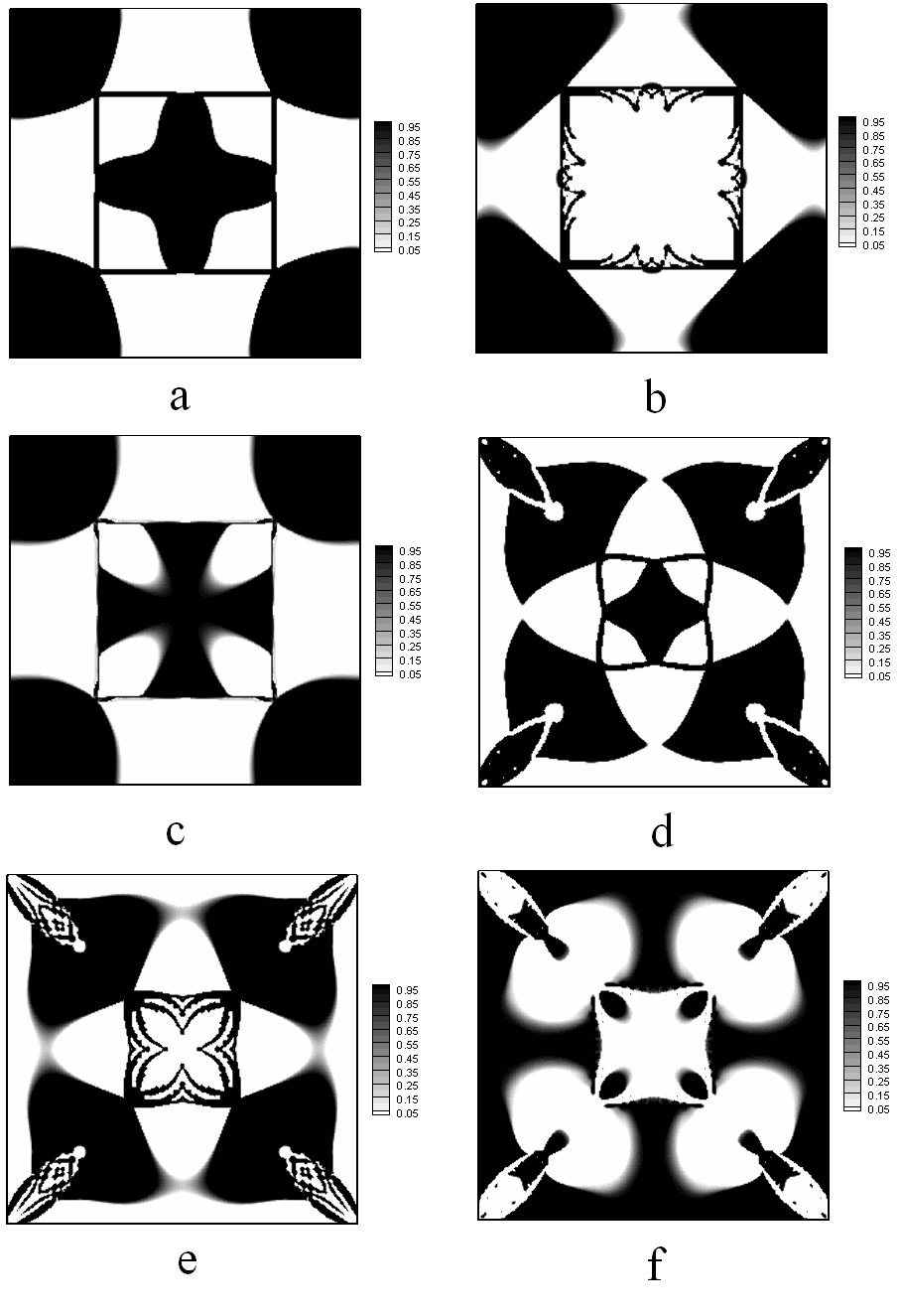
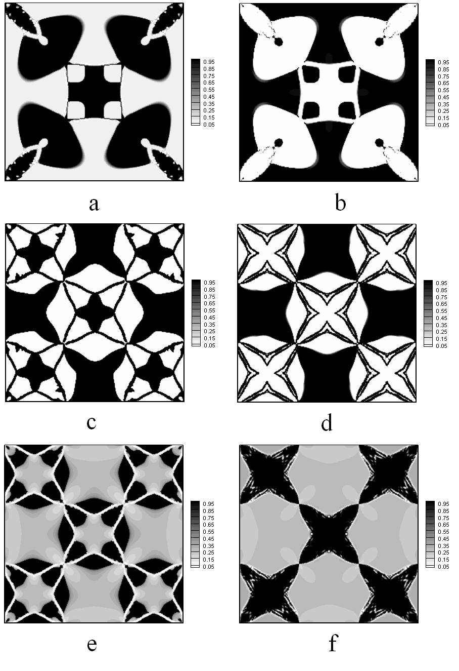
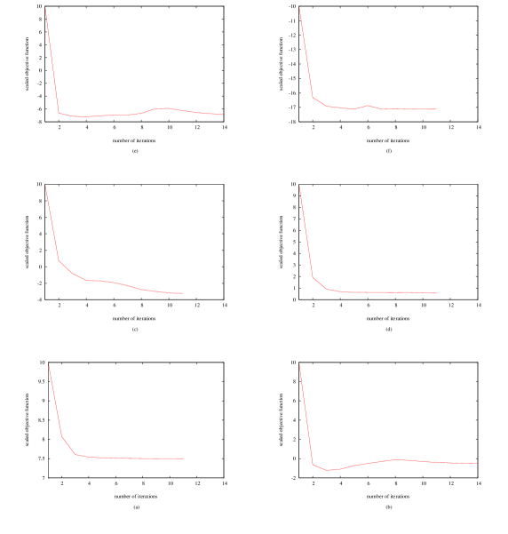
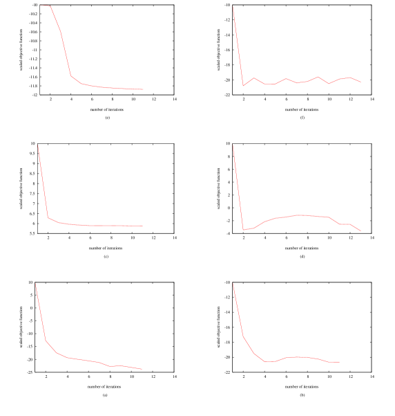
The resulted topologies related to examples 8.1- 8.14 are shown in Figures 1-3. Figures 4-6 show the variation of the objective functional as the optimization proceeds. Plots clearly show that, the presented method is enable to effectively reduce the objective functional in all cases and to move toward the optimal solution (if there be any). Moreover, in most of cases a near 0-1 topology is achieved. Therefore, we can conjecture about the existence of an optimal solution for problem $\mathtt{(P)}$ defined in this study. As it is clear from the plots, we do not have essentially a monotonic reduction in the objective functional value which is an expected result due to the use of a nonmonotonic line-search in our optimization algorithm (cf. [19]).

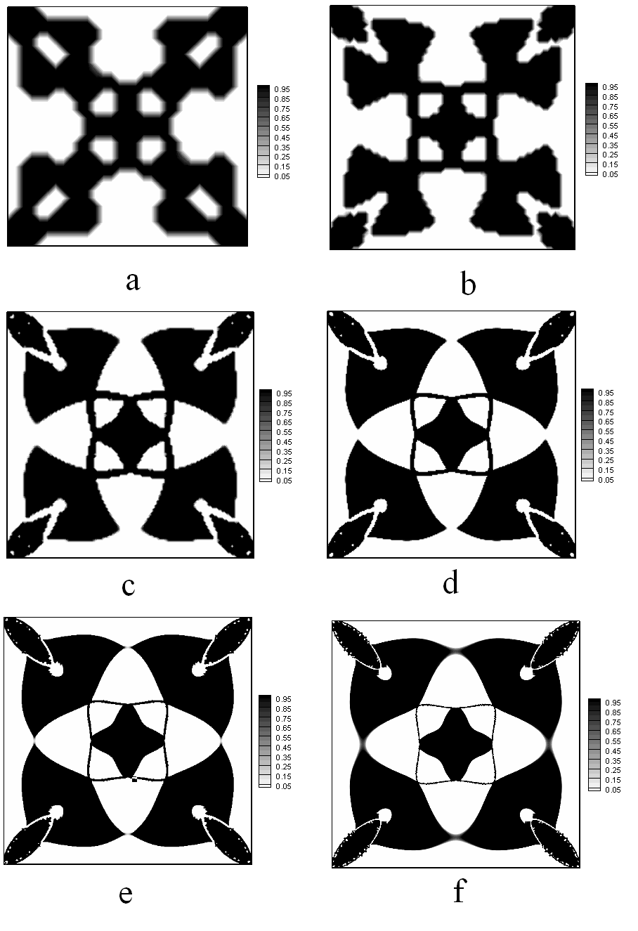
To study the stability and convergence of our method with respect to the grid refinement, example 8.4 is considered with grid resolutions: $2^{n}\times 2^{n},\ n=5,\cdots 10$. The resulted topologies related to this numerical experiment is shown in Figure 7. Plot shows that the macroscopic features of the topology have an excellent convergence. Moreover, the microscopic features follows the same trend without topological instability. Therefore, we can conjecture on the well-posedness and stability of the applied numerical method. Notice that, a micro-scale topological convergence is generally not expected due to this well-known fact that by the grid refinement the optimal solutions tend to form smaller and smaller microstructures (cf. [2]).

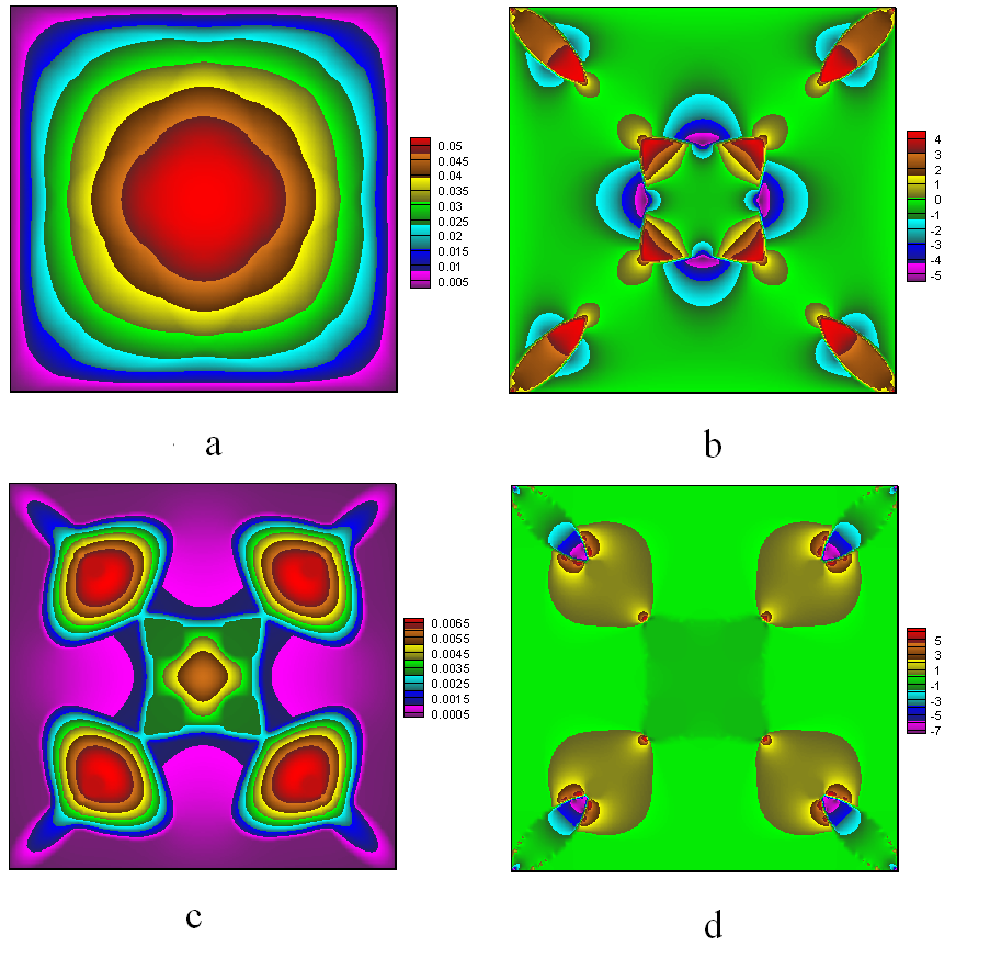
To make sense about the direct and adjoint fields at optimal solutions, the direct and adjoint fields at the optimal solution corresponding to examples 8.4 and 8.8 are plotted in Figure 8.

Figure 1. Optimal design in two spatial dimensions: a-f are related to the final topologies of examples 8.1-8.6 respectively.

Figure 2. Optimal design in two spatial dimensions: a-f are related to the final topologies of examples 8.7-8.12 respectively.

Figure 3. Optimal design in two spatial dimensions: a and b are related to the final topologies of examples 8.13 and 8.14 respectively.

Figure 4. Optimal design in two spatial dimensions: the objective function history, a-f are related to examples 8.1-8.6 respectively.

Figure 5. Optimal design in two spatial dimensions: the objective function history, a-f are related to examples 8.7-8.12 respectively.

Figure 6. Optimal design in two spatial dimensions: the objective function history, a and b are related to examples 8.13 and 8.14 respectively.

Figure 7. Optimal design in two spatial dimensions: the grid resolution study, a-f are related to the final topologies computed on the grid resolutions $2^{n}\times 2^{n}$, $n=5,\cdots,10$ respectively.

Figure 8. Optimal design in two spatial dimensions: the direct (left) and adjoint (right) fields at the final design for examples 8.4 (top) and 8.8 bottom.

To make sense about the computational cost of the presented approach, example 8.4 is considered with different conductivity ratios $\frac{k_{\alpha}}{k_{\beta}}=2,10,100$, and grid resolutions: $2^{n}\times 2^{n},\ n=5,\cdots 11$. Notice that for the conductivity ratio $100$, SIMP power $5$ is considered.

Table 1. Performance analysis: results include total optimization iterations (itero), total functional evaluation (nfunc), total gradient evaluation (ngard), total MGCG iterations (iterm) and total computational cost in second (cpu); for different conductivity ratios ($r_{k}=k_{\alpha}/k_{\beta}$) and different grid resolutions (grid).

grid	$r_{k}$	itero	nfunc	ngrad	iterm	cpu (sec)
$(2^{6})^{2}$	2	10	11	11	462	0.25
$(2^{7})^{2}$	2	10	11	11	484	2.15
$(2^{8})^{2}$	2	10	11	11	486	10.62
$(2^{9})^{2}$	2	11	12	12	528	46.76
$(2^{10})^{2}$	2	11	12	12	542	203.1
$(2^{11})^{2}$	2	13	12	12	612	1180.6
$(2^{6})^{2}$	10	10	11	11	792	0.36
$(2^{7})^{2}$	10	10	11	11	748	3.16
$(2^{8})^{2}$	10	10	11	11	836	16.25
$(2^{9})^{2}$	10	11	12	12	990	78.30
$(2^{10})^{2}$	10	11	12	12	1020	382.4
$(2^{11})^{2}$	10	14	15	15	1172	1905.1
$(2^{6})^{2}$	100	10	11	11	1430	0.56
$(2^{7})^{2}$	100	10	11	11	1716	6.49
$(2^{8})^{2}$	100	10	11	11	1958	35.05
$(2^{9})^{2}$	100	12	13	13	3014	220.7
$(2^{10})^{2}$	100	12	13	13	4940	1573.5
$(2^{11})^{2}$	100	14	15	15	6582	9941.1

Results of this numerical experiment are shown in Table 1. Table illustrates that the number of optimization cycles has a little dependency on the grid resolution and the conductivity ratio. The number of MGCG iterations is increased by increasing the conductivity ratio, $r_{k}$. But for a fixed $r_{k}$, the number of MGCG iterations is almost independent from the grid resolution, which show the reliability of this solver for large-scale problems. The reported computational cost illustrates the excellent performance of the applied numerical strategy in this study. To the best of our knowledge such a large number of design parameters ($2^{22}$) is not reported in literature of topology optimization so far.

8.2. Three dimensional results

In this section we show the success of the presented method in three spatial dimensions. For this purpose the following example is considered on grid resolutions: $2^{n}\times 2^{n}\times 2^{n}$, $n=5,6,7$.

Example 8.15.

$k_{\alpha}=2$, $k_{\beta}=1$, $q=1$, $g(\textbf{x})=1$, $u_{0}(\textbf{x})=0$, $a=-1$, $b=0$, $c=1$, and assuming $\kappa_{0}=-3$, the characteristic function $\chi(\mathcal{D})$ is defined as

$$\chi(\mathcal{D})=\left\{\begin{array}[]{rrr}1&\texttt{if}&\kappa_{\varepsilon}(\textbf{x})\leq\kappa_{0}\\ 0&\texttt{if}&\kappa_{\varepsilon}(\textbf{x})>\kappa_{0}\end{array}\right.$$

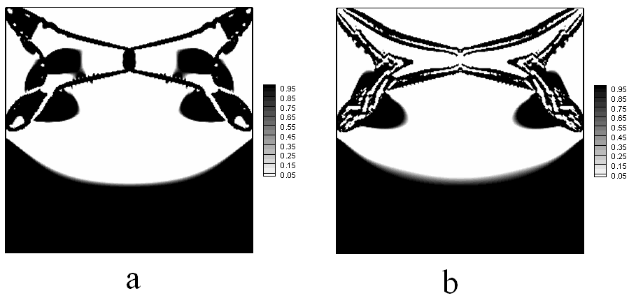
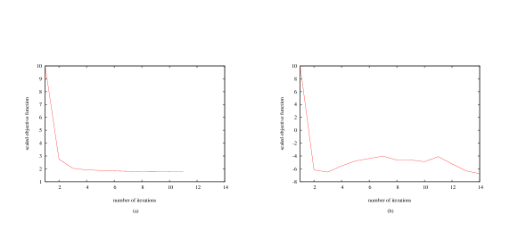
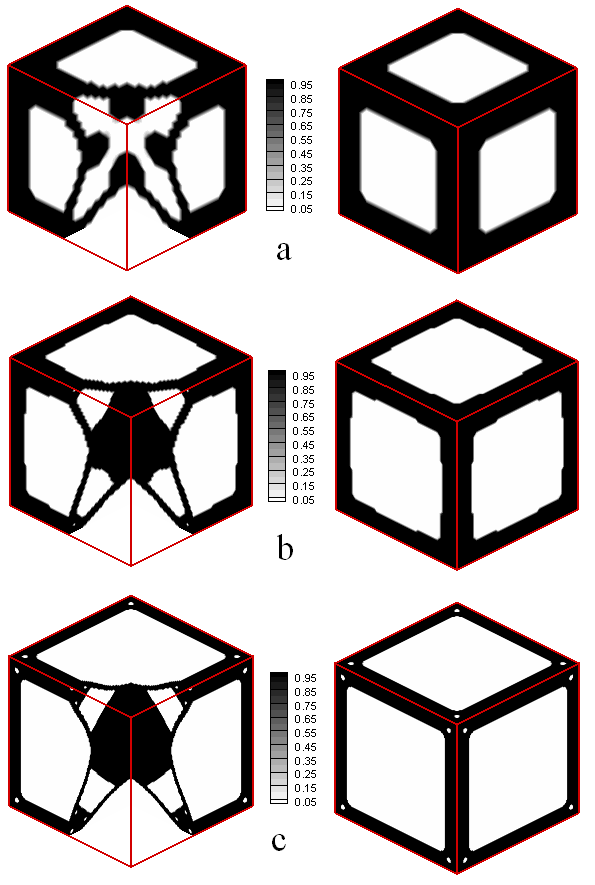
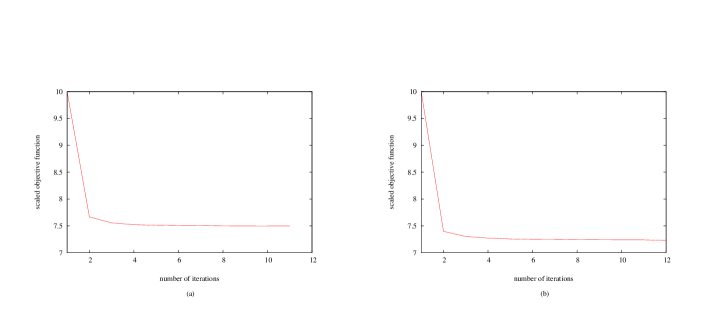
Figures 9 and 10 show the final topologies and objective function history corresponding to three dimensional numerical examples. In all cases the number of optimization iterations was below 13 and the number of objective functional and its gradient evaluation was equal. Plots illustrate the convergence and stability of the presented method in three spatial dimensions too.

Figure 9. Optimal design in three spatial dimensions: a-c are related to the final topologies computed on the grid resolutions $2^{n}\times 2^{n}\times 2^{n}$, $n=5,6,7$ respectively.

Figure 10. Optimal design in three spatial dimensions: the objective function history, a and b are related to grid resolutions $2^{6}\times 2^{6}\times 2^{6}$ and $2^{7}\times 2^{7}\times 2^{7}$ respectively.

9. Summary

The idea of posing control on the second order derivatives of the PDEs solutions is introduced in this study. To be specific, a topology optimization problem corresponding to the Poisson equation in which the objective functional is a nonlinear function of first and second order field derivatives is considered. Introducing some functional regularization tools, the (approximate) first order necessary optimality conditions is derived and is numerical solved using an appropriate gradient descent method. Numerical results are provided for a variety of test cases in two and three spatial dimensions. The Numerical results in this study, confirms the stability, convergence and efficiency of the presented approach. In fact, the numerical results answer to our quest in this study; the possibility of posing some degrees of control on the second order derivatives.

References

- [1] D. Adalsteinsson and JA Sethian. The Fast Construction of Extension Velocities in Level Set Methods. Journal of Computational Physics, 148(1):2–22, 1999.
- [2] G. Allaire. Shape optimization by the homogenization method. New York, Springer-Verlag, 2002., 2002.
- [3] G. Allaire. Numerical analysis and optimization: an introduction to mathematical modelling and numerical simulation. Translated by: Craig, A., Oxford University Press, USA, 2007.
- [4] M.P. Bendsoee and O. Sigmund. Topology Optimization: theory, methods and applications. Springer, 2004.
- [5] D.P. Bertsekas. Constrained optimization and Lagrange Multiplier methods. Academic Press, 1982.
- [6] T.B. Boykin. Derivatives of the Dirac delta function by explicit construction of sequences. American Journal of Physics, 71:462, 2003.
- [7] J.F. Colombeau. Multiplication of distributions. Bull. Amer. Math. Soc, 23:251–268, 1990.
- [8] I. Ekeland and R. Temam. Convex analysis and variational problems. SIAM, 1976.
- [9] L.C. Evans and R.F. Gariepy. Measure Theory and Fine Properties of Functions. CRC Press, 1992.
- [10] W.H. Fleming and R. Rishel. An integral formula for total gradient variation. Archiv der Mathematik, 11(1):218–222, 1960.
- [11] A. Gersborg-Hansen, M.P. Bendsøe, and O. Sigmund. Topology optimization of heat conduction problems using the finite volume method. Structural and Multidisciplinary Optimization, 31(4):251–259, 2006.
- [12] Y. Giga. Surface Evolution Equations: A Level Set Approach. Birkhäuser, 2006.
- [13] K. Ito and K. Kunisch. Lagrange Multiplier Approach to Variational Problems and Applications. SIAM, Philadelphia, 2008.
- [14] J.L. Lions. Optimal Control of Systems Governed by Partial Differential Equations, vol. 170 of Grundlehren Math. Wiss, 1971.
- [15] S. Osher and R.P. Fedkiw. Level Set Methods and Dynamic Implicit Surfaces. Springer, 2003.
- [16] JA Sethian. Fast Marching Methods. SIAM Review, 41(2):199–235, 1999.
- [17] O. Tatebe. The multigrid preconditioned conjugate gradient method. In Sixth Copper Mountain Conference on Multigrid Methods, pages 621–634, 1993.
- [18] R. Tavakoli. On the prediction of shrinkage defects by thermal criterion functions. Arxiv preprint arXiv:1005.2706, 2010.
- [19] R. Tavakoli and H. Zhang. A nonmonotone spectral projected gradient method for large-scale topology optimization problems. Arxiv preprint arXiv:1006.0561, 2010.
- [20] G. Temple. The Theory of Generalized Functions. Proceedings of the Royal Society of London. Series A, Mathematical and Physical Sciences (1934-1990), 228(1173):175–190, 1955.