A counterexample showing the semi-explicit Lie-Newmark algorithm is not variational

Abstract

This paper presents a counterexample to the conjecture that the semi-explicit Lie-Newmark algorithm is variational. As a consequence the Lie-Newmark method is not well-suited for long-time simulation of rigid body-type mechanical systems. The counterexample consists of a single rigid body in a static potential field, and can serve as a test of the variational nature of other rigid-body integrators.

Keywords: rigid body, long-time simulation, Newmark algorithm

MSC 2000: 65P10

1 Introduction

In this paper we will focus on the dynamics of a rigid body in a static potential field. To describe this system, denote by $Q(t)\in\operatorname{SO}(3)$, $W(t)={{\left[W_{1}(t)\ W_{2}(t)\ W_{3}(t)\right]}}^{T}\in\mathbb{R}^{3}$, and $\mathbb{I}=\text{diag}(I_{1},I_{2},I_{3})\in\mathbb{R}^{3\times 3}$ the configuration, body angular velocity and inertia matrix of the body, respectively. Let $\tau:\operatorname{SO}(3)\to\mathbb{R}^{3}$ be the torque acting on the body and $\ \widehat{\,}:\,\mathbb{R}^{3}\to\mathbb{R}^{3\times 3}$ be the hat map

$$\widehat{W}=\begin{bmatrix}0&-W_{3}&W_{2}\\ W_{3}&0&-W_{1}\\ -W_{2}&W_{1}&0\end{bmatrix}\!.$$

In terms of this notation, the governing equations are

$$\dot{Q}\!\!\!\!\!\!\!\!\! =Q\widehat{W}$$ (1)

$$\mathbb{I}\,\dot{W}\!\!\!\!\!\!\!\!\! =\mathbb{I}\,W\times W+\tau(Q),$$ (2)

with initial conditions $Q(0)=Q_{0}\in\operatorname{SO}(3)$ and $W(0)=W_{0}\in\mathbb{R}^{3}$. We assume this rigid body is derivable from a Lagrangian $L:\operatorname{SO}(3)\times\mathbb{R}^{3}\to\mathbb{R}$ of the form

$$L(Q,W)=T(W)-U(Q)\;\hbox{,}$$ (3)

where $T(W)=\frac{1}{2}W^{T}\mathbb{I}\,W$ and $U(Q)$ are the kinetic and potential energy of the body, respectively. This assumption implies that the torque in (2) can be computed from the directional derivative of $U$ at $Q$ in the direction $Q\widehat{y}$:

$$\tau(Q)^{T}y=-\operatorname{\textrm{D}}U(Q)\cdot Q\,\hat{y}\;\hbox{,}~{}~{}~{}y\in\mathbb{R}^{3}\;.$$

Notice that the total energy is separable and $T(-W)=T(W)$. The exact flow of (2) possesses certain structure such as total energy preservation, time-symmetry, and symplecticity. Moreover, the path $Q$ lies on a configuration manifold $\operatorname{SO}(3)$ which possesses a Lie-group structure.

This paper investigates the long-run behavior of two integrators for (2): the Lie-Newmark [SVQ88, SW91] and Lie-Verlet methods [BRM08]. Both methods are semi-explicit, second-order accurate and symmetric. They are also ‘Lie group methods’ because they respect the Lie group structure of the configuration manifold [IMKNZ00]. Moreover, the complexity and implementation of the two methods is quite similar. The main difference between the integrators is that the Lie-Verlet method is designed to be variational, whereas the Lie-Newmark method is not.

Variational integrators are time-integrators adapted to the structure of mechanical systems [MW01, LMOW04a, LMOW04b]. They are symplectic, and in the presence of symmetry, momentum preserving. The theory of variational integrators includes discrete analogues of Hamilton’s principle, Noether’s theorem, the Euler-Lagrange equations, and the Legendre transform. The variational nature of Lie-Verlet guarantees its excellent long-time behavior. In fact, one can prove this. The basic idea of the proof is to show that a trajectory of a variational integrator is interpolated by a level set of a ‘modified’ energy function nearby the true energy [BG94, Rei99, HLW06]. This implies that a trajectory of the variational integrator is confined to these level sets for the duration of the simulation. As a consequence variational integrators nearly preserve the true energy and exhibit linear growth in global error. For these reasons variational integrators are well-suited for long-time simulation.

Even though the Lie-Newmark integrator is not designed to be variational, this does not rule out the possibility that the algorithm is variational in a subtle way like classical Newmark. The classical Newmark family of algorithms are widely used integrators in computational mechanics (for an expository treatment see, e.g., Chapter 9 of [Hug87]). They were first proposed in [New59], but it took more than forty years for their variational nature to be established in [KMOW00]. Specifically, Kane et al. proved that a trajectory of the classical Newmark method is shadowed by a trajectory of a variational algorithm. In other words the Newmark integrators are not symplectic, but conjugate symplectic [HLW06]. The possibility that Lie-Newmark could be analogously variational (or conjugate symplectic) was supported by recent numerical evidence showing that the Lie-Newmark algorithm exhibits excellent behavior akin to classical Newmark [KE05]. Based on these experiments, Krysl and Endres conjectured that the Lie-Newmark algorithm is variational.

This paper disproves this conjecture. In particular, the paper presents a simple numerical counterexample showing that the Lie-Newmark method exhibits systematic energy drift. In contrast, the Lie-Verlet method nearly preserves the true energy and exhibits the qualitative properties one expects of a variational integrator. In summary, the Lie-Verlet method is well-suited for long-time simulation of rigid body-type mechanical systems, while the Lie-Newmark method is not.

The paper is organized as follows. The algorithms used in the paper are stated in §2 and the numerical ‘stress test’ carried out in §3. In §4 we provide concluding remarks including other applications of this numerical ‘stress test.’ Along with this paper, we have released a simple Matlab implementation of the presented algorithms. This release can be retrieved from the Matlab Central File Exchange.

2 Integrators

Lie-Newmark

The Lie-Newmark family of integrators was proposed more than twenty years ago in [SVQ88]. These methods consist of a Newmark-style discretization of (2) and a discretization of (1) that ensures the configuration update remains on $\operatorname{SO}(3)$. These methods were motivated by the need to develop conserving algorithms that can efficiently simulate the structural dynamics of rods and shells. For example, consider simulating large deformations of a three-dimensional finite-strain rod model. The rod is typically discretized using $N$ copies of $\mathbb{R}^{3}\times\operatorname{SO}(3)$ where $N$ is the number of discretization points along the line of centroids of the rod. The configuration of the rod at each point along the line of centroids is specified by an element of $\operatorname{SO}(3)$. The dynamical behavior of the rod can then be estimated by simulating the dynamics of $N$ rigid bodies with torques due to elastic coupling between bodies.

This paper focuses on a specific member of the Lie-Newmark family tested in [KE05]. This member is the Lie group analog of the so-called explicit Newmark method on vector spaces (see Chapter 9 of [Hug87]). In molecular dynamics the explicit Newmark method is known as the Verlet integrator [HLW06]. Given $(Q_{k},W_{k})\in\mathbb{R}^{3}\times\operatorname{SO}(3)$ and time-stepsize $h$, the Lie-Newmark algorithm determines $(Q_{k+1},W_{k+1})$ by the following iteration rule:

$$W_{k+\frac{1}{2}}=W_{k}+\frac{h}{2}\mathbb{I}^{-1}{\left(\mathbb{I}\,W_{k}\times W_{k}+\tau(Q_{k})\right)}\;\hbox{,}$$ (4)

$$Q_{k+1}=Q_{k}\,\text{cay}(hW_{k+\frac{1}{2}})\;\hbox{,}$$ (5)

$$W_{k+1}=W_{k+\frac{1}{2}}+\frac{h}{2}\mathbb{I}^{-1}{\left(\mathbb{I}\,W_{k+1}\times W_{k+1}+\tau(Q_{k+1})\right)}\;.$$ (6)

Here we have introduced the Cayley map $\text{cay}:\mathbb{R}^{3}\to\operatorname{SO}(3)$:

$$\text{cay}(x)=I+\frac{4}{4+|x|}\hat{x}+\frac{2}{4+|x|}{\hat{x}}^{2}\;\hbox{,}~{}~{}~{}x\in\mathbb{R}^{3}\;\hbox{,}$$ (7)

where $I$ is the identity matrix. The Cayley map is a second-order approximation of the exponential map on $\operatorname{SO}(3)$. There are other maps one can use in place of the Cayley map in (5) (see, e.g., [BR07, §5.4]), but the Cayley map is known to be very computationally efficient in practice. This integrator is semi-explicit because (4)-(5) involve explicit updates, and (6) is only implicit in the angular velocity and not in the torque. Hence, the implicitness of the Lie-Newmark method is not severe. It is also symmetric and second-order accurate.

Lie-Verlet

The Lie-Verlet integrator was proposed in [BRM08] and based on the theory of discrete and continuous Euler-Poincaré systems [MPS98, MS93]. The method is closely related to, but different from the RATTLE method for constrained mechanical systems [HLW06].

Given $(Q_{k},W_{k})\in\mathbb{R}^{3}\times\operatorname{SO}(3)$ and time-stepsize $h$, the Lie-Verlet algorithm determines $(Q_{k+1},W_{k+1})$ by the following iteration rule:

$$W_{k+\frac{1}{2}}\!=\!W_{k}+\frac{h}{2}\mathbb{I}^{-1}\!\!{\left[\mathbb{I}\,W_{k+\frac{1}{2}}\!\times\!W_{k+\frac{1}{2}}-\frac{h}{2}{\left(W_{k+\frac{1}{2}}^{T}\mathbb{I}\,W_{k+\frac{1}{2}}\right)}W_{k+\frac{1}{2}}+\tau(Q_{k})\right]}\;\hbox{,}$$ (8)

$$Q_{k+1}=Q_{k}\,\text{cay}(hW_{k+\frac{1}{2}})\;\hbox{,}$$ (9)

$$W_{k+1}\!=\!W_{k+\frac{1}{2}}\!\!+\!\frac{h}{2}\mathbb{I}^{-1}\!\!{\left[\mathbb{I}\,W_{k+\frac{1}{2}}\!\!\times\!W_{k+\frac{1}{2}}\!+\!\frac{h}{2}\!{\left(W_{k+\frac{1}{2}}^{T}\mathbb{I}\,W_{k+\frac{1}{2}}\right)}\!W_{k+\frac{1}{2}}\!\!+\tau(Q_{k+1})\right]}\!.$$ (10)

Similar to the Lie-Newmark method, this algorithm is symmetric, semi-explicit and second-order accurate. In particular, the updates in (9) and (10) are explicit, and the implicitness in (8) does not involve the torque. We emphasize the Lie-Verlet integrator is variational and refer the reader to [BRM08] for a proof of this result.

3 Numerical Counterexample

This section describes a numerical experiment showing that the semi-explicit Lie-Newmark integrator (6) exhibits systematic drift in total energy. Such drift implies that the method is not a conjugate symplectic integrator for (2), and hence, is not variational. The numerical counterexample we discuss is strongly inspired by a numerical experiment reported in [FHP04, §4.4]. That paper shows systematic energy drift along an orbit of a fourth-order accurate, implicit, and symmetric Lobatto IIIB integrator when applied to a spring pendulum with exterior forces.

Preliminaries

Let $I\in\operatorname{SO}(3)$ be the identity matrix, and in terms of which, define the function $\textrm{dist}:\operatorname{SO}(3)\times\operatorname{SO}(3)\rightarrow\mathbb{R}$ as

$$\textrm{dist}(Q_{1},Q_{2})\stackrel{{\scriptstyle\mbox{\tiny def}}}{{=}}\sqrt{2\,\textrm{tr}(I-Q_{1}^{T}Q_{2})}\,.$$ (11)

Let $\|\cdot\|_{F}$ denote the Frobenius matrix norm. We recall that $\|A\|_{F}:=\sqrt{\textrm{tr}(A^{T}A)}$ for $A\in\mathbb{R}^{n\times n}$. It is straightforward to verify that $\textrm{dist}(\cdot,\cdot)$ is a metric on $\operatorname{SO}(3)$ induced by the Frobenius norm using the identity

$$\|Q_{2}-Q_{1}\|^{2}_{F}=2\,\textrm{tr}(I-Q_{1}^{T}Q_{2})\,.$$

For the numerical experiment, consider a single rigid body in a static field defined by the potential energy function $U_{\alpha}:\operatorname{SO}(3)\rightarrow\mathbb{R}$ given by:

$$U_{\alpha}(Q)=\bigl{(}\textrm{dist}(Q,I)-1\bigr{)}^{2}-\frac{\alpha}{\textrm{dist}(Q,Q_{m})}\;.$$ (12)

The first term in the right hand side of (12) is a bounded potential which attains its minimum value at $Q\in\operatorname{SO}(3)$ satisfying $\textrm{dist}(Q,I)=1$. The second term is an unbounded potential that generates an attraction toward the configuration $Q_{m}\in\operatorname{SO}(3)$. The parameter $\alpha$ is a tuning parameter.

For $\alpha=0$, the potential energy $U_{\alpha=0}$ achieves its minimum value on the two-dimensional surface

$$S\stackrel{{\scriptstyle\mbox{\tiny def}}}{{=}}\{Q\in\operatorname{SO}(3):\textrm{dist}(Q,I)=1\}\;.$$

This implies that the set $S\times\{0\}\subset\operatorname{SO}(3)\times\mathbb{R}^{3}$ is a (locally) stable set in the sense of Lyapunov for the dynamics of the rigid body. One proves this fact using as Lyapunov function the energy

$$E(Q,W)=T(W)+U_{\alpha=0}(Q)$$

and noting that the set $\{(Q,W)\in\operatorname{SO}(3)\times\mathbb{R}^{3}\;|\;E(Q,W)\leq\bar{E}\}$ is compact for every $\bar{E}\geq 0$.

For $\alpha>0$, the set $S$ gets perturbed by the unbounded attractive potential. On this perturbed energy landscape, the rigid body experiences an attraction toward the configuration $Q_{m}$. Yet, if we place the attraction point $Q_{m}$ sufficiently far from the set $S$ and choose the tuning parameter $\alpha>0$ sufficiently small, the set $S$ gets only slightly perturbed into a new set, that we label $S_{\alpha}$. Furthermore, the set $S_{\alpha}\times\{0\}\subset\operatorname{SO}(3)\times\mathbb{R}^{3}$ is locally Lyapunov stable like the unperturbed set $S\times\{0\}$.

In summary, we can design $U_{\alpha}$ so that the true solution conserves a compact energy function when initialized in a neighborhood of the set $S_{\alpha}\times\{0\}$. This conserved quantity implies that the true solution is confined to this neighborhood. This property will be preserved by the Lie-Verlet integrator since it is variational. Recall that a variational integrator is interpolated by a level set of a ‘modified’ energy function nearby the true energy [BG94, Rei99, HLW06]. This implies that a trajectory of the variational integrator is confined to a neighborhood of $S_{\alpha}\times\{0\}$ for the duration of the simulation. Next we show that the Lie-Newmark integrator exhibits systematic drift in this energy function.

Numerical ‘Stress Test’

Now we are in position to describe the numerical counterexample. Select the inertia matrix to be

$$\mathbb{I}=\begin{bmatrix}2&0&0\\ 0&2&0\\ 0&0&4\end{bmatrix}\;\hbox{,}$$

and the tuning parameter to be $\alpha=0.3$. Place the attraction point at

$$Q_{m}=\mathop{\hbox{\rm{exp}}}\nolimits(v_{m})\;\hbox{,}~{}~{}~{}v_{m}=\frac{1}{\sqrt{2}}\begin{bmatrix}2.5\\ 0\\ 2.5\end{bmatrix}\;.$$

Here $\mathop{\hbox{\rm{exp}}}\nolimits:\mathbb{R}^{3}\to\operatorname{SO}(3)$ is the exponential map

$$\mathop{\hbox{\rm{exp}}}\nolimits(x)=I+\frac{\mathop{\hbox{\rm{sin}}}\nolimits(|x|)}{|x|}\hat{x}+\frac{1-\mathop{\hbox{\rm{cos}}}\nolimits(|x|)}{|x|^{2}}\hat{x}^{2}\;\hbox{,}~{}~{}~{}x\in\mathbb{R}^{3}\;.$$

The initial condition $(Q_{0},W_{0})\in\mathbb{R}^{3}\times\operatorname{SO}(3)$ is selected so that $\textrm{dist}(Q_{0},I)$ is nearly one. Specifically, select the initial configuration and angular velocity to be

$$Q_{0}=\mathop{\hbox{\rm{exp}}}\nolimits(v_{0})\;\hbox{,}~{}~{}~{}v_{0}=\begin{bmatrix}0\\ 0.7227\\ 0\end{bmatrix}\;\hbox{,}~{}~{}~{}W_{0}=\begin{bmatrix}0\\ 0\\ 0.625\end{bmatrix}\;.$$

In the numerical experiment we test the two integrators, Lie-Newmark (NMB) and velocity Lie-Verlet (VLV), on a long time interval $[0,15000]$. The energy error obtained with a time-stepsize $h=0.125$ is shown in Figure 1(a). The experiment was repeated with a time-stepsize $h=0.25$ and results are reported in Figure 1(b). A systematic drift for the NMB scheme can be observed in both cases. The drift appears linear in the time span $T$ and quadratic in the time-stepsize $h$. We abbreviate this fact by saying the total energy error behaves like $\mathcal{O}(Th^{2})$. No energy drift is observed for the VLV scheme. We have also tested the Lie-Newmark method with the Cayley map in (5) replaced by the exponential map. Systematic energy drift is observed in that case too.

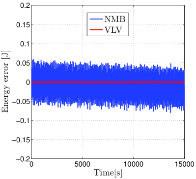
(a) h = 0.125

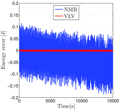
(b) h = 0.25

Figure 1: This figure shows the energy error of the Lie-Newmark (NMB) and velocity Lie-Verlet (VLV) algorithms for the rigid body in the potential energy landscape defined by (12) for two different timesteps. NMB exhibits a systematic energy drift. On the other hand, the energy error of VLV method remains bounded as predicted by theory. The initial conditions and parameters used are provided in the text.

The trajectory generated by Lie-Newmark for time-stepsize $h=0.25$ is shown in the axis/angle representation of $\operatorname{SO}(3)$ in Figure 2. The semi-transparent surfaces correspond to isosurfaces of the potential energy (12).

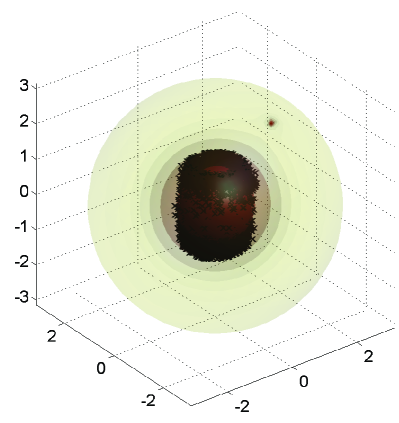
Figure 2: This figure shows a trajectory generated by the Lie-Newmark integrator operated at time-stepsize $h=0.25$ projected on the axis/angle representation of $\operatorname{SO}(3)$. The initial conditions and parameters used are provided in the text. The semi-transparent surfaces are level sets of the potential energy (12). The darker shading corresponds to lower potential energy. The dot in the figure corresponds to the attraction point $Q_{m}\in\operatorname{SO}(3)$ of the potential energy.

The time-precision diagrams, shown in Figures 3(a) and 3(b) confirm that NMB and VLV are second-order accurate. Observe from the figures that the slope of the two lines denoting the global error is $\mathcal{O}(h^{2})$. The diagrams have been generated by computing the global error in the configuration and angular velocity evaluated at $T=5$. The simulations have been performed for a variety of time-stepsizes as indicated in the figures. The reference solution was computed using the function ode45 in Matlab, with an absolute tolerance $10^{-14}$ and relative tolerance $2\cdot 10^{-14}$.

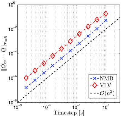
(a) Configuration.

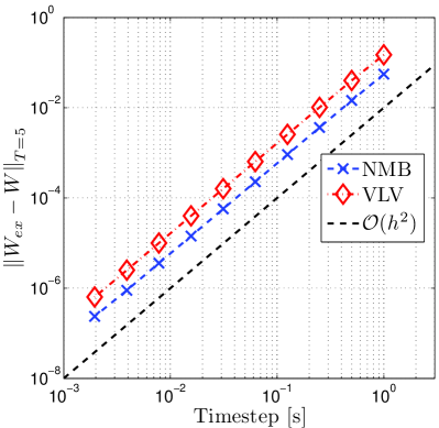
(b) Body angular velocity.

Figure 3: This figure shows the global error of the Lie-Newmark (NMB) and velocity Lie-Verlet (VLV) algorithms. The global error is evaluated in configuration and body angular velocity at a physical time of $T=5$ for a variety of time-stepsizes. We use as a reference solution an integration of (2) using the Matlab function ode45 with low tolerance. Observe that both integrators are second-order accurate.

4 Conclusion

The Lie-Newmark method was proposed as a generalization of the explicit Newmark algorithm to Lie groups [SVQ88]. However, unlike its counterpart on vector spaces, this paper shows that the Lie-Newmark method does not possess excellent long-time behavior when applied to a rigid body in a potential force field. In particular, the paper presents a numerical experiment showing the Lie-Newmark integrator exhibits systematic energy drift with an $\mathcal{O}(Th^{2})$ behavior. In contrast, the Lie-Verlet method, which is variational by construction, does not exhibit energy drift as predicted by theory. Since the two methods are semi-explicit, symmetric and computationally similar to implement, we conclude that the Lie-Verlet method is better suited for long-time simulation of rigid body-type systems.

As a final remark, we note that the numerical example appearing in this paper can serve as a test for symplecticity of other rigid body integrators. For instance, in Appendix A we show non-symplecticity of the ‘explicit’ Lie-Midpoint algorithm proposed in [Kry05].

Appendix A Non-Symplecticity of Explicit Lie-Midpoint Algorithm

In this section the LIEMID[EA] algorithm is subjected to the numerical ‘stress test’ described in §3. This algorithm was thought to be a symplectic-momentum integrator in [Kry05]. However, the test reveals that the integrator is not conjugate symplectic.

Given $(Q_{k},W_{k})\in\mathbb{R}^{3}\times\operatorname{SO}(3)$ and time-stepsize $h$, the LIEMID[EA] algorithm determines $(Q_{k+1},W_{k+1})$ by the following iteration rule:

$$\Theta_{k+\frac{1}{2}}\!=\frac{h}{2}\mathbb{I}^{-1}\mathop{\hbox{\rm{exp}}}\nolimits(-\frac{1}{2}\widehat{\Theta}_{k+\frac{1}{2}})(\mathbb{I}W_{k}+\frac{h}{2}\tau(Q_{k}))\;\hbox{,}$$ (13)

$$Q_{k+\frac{1}{2}}=Q_{k}\mathop{\hbox{\rm{exp}}}\nolimits(\widehat{\Theta}_{k+\frac{1}{2}})\;\hbox{,}$$ (14)

$$W_{k+\frac{1}{2}}\!=\!\mathbb{I}^{-1}\mathop{\hbox{\rm{exp}}}\nolimits(-\widehat{\Theta}_{k+\frac{1}{2}})(\mathbb{I}W_{k}+\frac{h}{2}\tau(Q_{k}))\;\hbox{,}$$ (15)

$$\Theta_{k+1}=\frac{h}{2}\mathbb{I}^{-1}\mathop{\hbox{\rm{exp}}}\nolimits(-\frac{1}{2}\widehat{\Theta}_{k+1})(\mathbb{I}W_{k+\frac{1}{2}})\;\hbox{,}$$ (16)

$$Q_{k+1}\!=Q_{k+\frac{1}{2}}\mathop{\hbox{\rm{exp}}}\nolimits(\widehat{\Theta}_{k+1})\;\hbox{,}$$ (17)

$$W_{k+1}\!=\!\mathbb{I}^{-1}(\mathop{\hbox{\rm{exp}}}\nolimits(-\widehat{\Theta}_{k})\mathbb{I}W_{k+\frac{1}{2}}+\frac{h}{2}\tau(Q_{k+1}))\!\;.$$ (18)

This integrator is more implicit than the semi-explicit Lie-Newmark and Lie-Verlet methods introduced in §2. In particular, the updates (13) and (16) are both implicit. Hence, the algorithm involves two nonlinear solves per step, unlike the Lie-Newmark and Lie-Verlet methods which involve one nonlinear solve per step. The four remaining updates are explicit. This algorithm was derived as a composition of a half-step of a first-order Lie-midpoint method and its adjoint [Kry05]. As an immediate consequence, the method is symmetric and second-order accurate. However, the numerical ‘stress test’ shows that this integrator is not conjugate symplectic.

The stress test described in §3 is carried out on LIEMID[EA]. The parameter values and initial conditions provided in §3 are used. The time interval of integration is set to be $[0,15000]$. The energy error obtained on this time interval with a time-stepsize $h=0.125$ is shown in Figure 4(a). The experiment was repeated with a time-stepsize $h=0.25$ and results are reported in Figure 4(b). A systematic drift for the LIEMID[EA] scheme can be observed in both cases. The drift appears linear in the time span $T$ and quadratic in the time-stepsize $h$. We note that the drift of LIEMID[EA] is smaller than the drift exhibited by NMB. The time-precision diagrams, shown in Figures 5(a) and 5(b) confirm that LIEMID[EA] is second-order accurate.

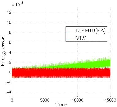
(a) h = 0.125

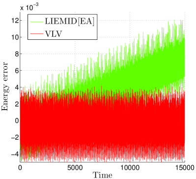
(b) h = 0.25

Figure 4: This figure shows the energy error of the Explicit Lie-Midpoint (LIEMID[EA]) and velocity Lie-Verlet (VLV) algorithms for the rigid body in the potential energy landscape defined by (12) for two different timesteps. LIEMID[EA] exhibits a systematic energy drift. On the other hand, the energy error of VLV method remains bounded as predicted by theory. The initial conditions and parameters used are provided in the text.

(a) Configuration.

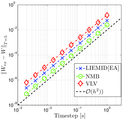
(b) Body angular velocity.

Figure 5: This figure shows the global error of the Explicit Lie-Midpoint (LIEMID[EA]), Lie-Newmark (NMB) and velocity Lie-Verlet (VLV) algorithms. The global error is evaluated in configuration and body angular velocity at a physical time of $T=5$ for a variety of time-stepsizes. We use as a reference solution an integration of (2) using the Matlab function ode45 with low tolerance. Observe that all the integrators are second-order accurate.

References

- [BG94] G. Benettin and A. Giorgilli. On the Hamiltonian interpolation of near to the identity symplectic mappings with applications to symplectic integration algorithms. J. Statist. Phys. 74, (1994), 1117–1143.
- [BR07] N. Bou-Rabee. Hamilton-Pontryagin Integrators on Lie Groups. Ph.D. thesis, California Institute of Technology, 2007.
- [BRM08] N. Bou-Rabee and J. E. Marsden. Hamilton-Pontryagin integrators on Lie groups. Foundations of Computational Mathematics 9, (2008), 197–219.
- [FHP04] E. Faou, E. Hairer, and T. Pham. Energy conservation with non-sympletic methods: examples and counter-examples. BIT Numerical Mathematics 44, (2004), 699–709.
- [HLW06] E. Hairer, C. Lubich, and G. Wanner. Geometric Numerical Integration, vol. 31 of Springer Series in Computational Mathematics. Springer, 2006.
- [Hug87] T. J. R. Hughes. The Finite Element Method. Prentice-Hall, 1987.
- [IMKNZ00] A. Iserles, H. Z. Munthe-Kaas, S. P. Nørsett, and A. Zanna. Lie-group methods. Acta Numerica 9, (2000), 1–148.
- [KE05] P. Krysl and L. Endres. Explicit Newmark/Verlet algorithm for time integration of the rotational dynamics of rigid bodies. International Journal for Numerical Methods in Engineering 62, (2005), 2154–2177.
- [KMOW00] C. Kane, J. E. Marsden, M. Ortiz, and M. West. Variational integrators and the Newmark algorithm for conservative and dissipative mechanical systems. Int. J. Numer. Methods Eng. 49, (2000), 1295–1325.
- [Kry05] P. Krysl. Explicit momentum-conserving integrator for dynamics of rigid bodies approximating the midpoint lie algorithm. International Journal for Numerical Methods in Engineering 63, (2005), 2171 2193.
- [LMOW04a] A. Lew, J. E. Marsden, M. Ortiz, and M. West. An overview of variational integrators. In Finite Element Methods: 1970s and Beyond, 98–115. 2004.
- [LMOW04b] A. Lew, J. E. Marsden, M. Ortiz, and M. West. Variational time integrators. Int. J. Numer. Methods Eng. 60, (2004), 153–212.
- [MPS98] J. E. Marsden, S. Pekarsky, and S. Shkoller. Discrete Euler-Poincaré and Lie-Poisson equations. Nonlinearity 12, (1998), 1647–1662.
- [MS93] J. E. Marsden and J. Scheurle. The reduced Euler-Lagrange equations. Fields Inst. Comm. 1, (1993), 139–164.
- [MW01] J. E. Marsden and M. West. Discrete mechanics and variational integrators. Acta Numerica 10, (2001), 357–514.
- [New59] N. M. Newmark. A method of computation for structural dynamics. ASCE J. of the Engineering Mechanics Division 36, (1959), 67–94.
- [Rei99] S. Reich. Backward error analysis for numerical integrators. SIAM J. Num. Anal. 36, (1999), 1549–1570.
- [SVQ88] J. C. Simo and L. Vu-Quoc. On the dynamics in space of rods undergoing large motions - a geometrically exact approach. Computer Methods in Applied Mechanics and Engineering 66, (1988), 125–161.
- [SW91] J. C. Simo and T. S. Wong. Unconditionally stable algorithms for rigid body dynamics that exactly preserve energy and momentum. International Journal for Numerical Methods in Engineering 31, (1991), 19–52.