Fast quantum algorithms for traversing paths of eigenstates
Abstract
Consider a path of non-degenerate eigenstates , , of unitary operators or Hamiltonians with minimum eigenvalue gap . The eigenpath traversal problem is to transform one or more copies of into . Solutions to this problem have applications ranging from quantum physics simulation to optimization. For Hamiltonians, the conventional way of doing this is by applying the adiabatic theorem. We give “digital” methods for performing the transformation that require no assumption on path continuity or differentiability other than the absence of large jumps. Given sufficient information about eigenvalues and overlaps between states on the path, the transformation can be accomplished with complexity , where is the angular length of the path and is a specified bound on the error of the output state. We show that the required information can be obtained in a first set of transformations, whose complexity per state transformed has an additional factor that depends logarithmically on a maximum angular velocity along the path. This velocity is averaged over constant angular distances and does not require continuity. Our methods have substantially better behavior than conventional adiabatic algorithms, with fewer conditions on the path. They also improve on the previously best digital methods and demonstrate that path length and the gap are the primary parameters that determine the complexity of state transformation along a path.
I Introduction
Most quantum algorithms exhibiting speedups are based on one of a small number of basic tools for quantum problem solving. These tools include phase estimation, which underlies quantum factoring, and amplitude amplification, which can be used to solve search problems. Another such tool is adiabatic state transformation (AST). Before finding applications in quantum algorithms, AST was used in classical algorithms for quantum physics simulation amara:qc1993a ; finnila:qc1994a ; kadowaki:qc1998a . It is now a key method for accessing low-energy states in proposed quantum simulations of physics, both in “digital” quantum algorithms based on the circuit model ortiz:qc2001a ; aspuru-guzik:qc2005a and in “analog” simulation techniques involving direct realization of Hamiltonians in systems such as optical lattices (see Ref. lewenstein:qc2007a ). The potential of AST was recognized in quantum computer science when it was proposed as a powerful heuristic for solving satisfiability problems farhi_quantum_2000 ; farhi:qc2001a . This led to the idea of adiabatic quantum computing (AQC), which involves encoding the output of any quantum algorithm in an adiabatically accessible ground state farhi_quantum_2000 ; aharonov_adiabatic_2003 . More recently, it has been shown that AST can be used for quantum speedups of Monte-Carlo algorithms somma_quantum_2008 ; wocjan_speedup_2008 .
We consider AST problems that involve transforming into , where these states are the endpoints of a path of states for . The are eigenstates of operators , which may be unitary or Hermitian. For simplicity, we focus on the unitary case . If is Hermitian, we define . The eigenphase of with respect to is and is assumed to be non-degenerate. The gap to the nearest other eigenphase is denoted by . We make no continuity assumptions on or . Thus, our formulation of the AST problem can accommodate cases where the path is discrete, parameterized by integers . It suffices to define for .
The complexity of the AST problem depends on the available capabilities and what we know about the path. We assume that we can prepare copies of , and that we can apply quantum-controlled instances of , both at unit cost. Additional information such as lower bounds on the gaps, eigenphase ranges and overlaps between the may be available. An important consequence of our results is that the main parameter that determines the complexity of an AST problem is the angular length of the path, which is defined as
| (1) |
If is differentiable in , then . For the purpose of making complexity statements, let . Given sufficient information about the overlaps between nearby states on the path, we show that the complexity of an AST problem is , where is a specified bound on the error with which is prepared. (Our complexity statements hide constants that apply uniformly for all , and .) The dependence on and is within a factor of at most of optimal. That is, there are classes of AST problems for which every algorithm uses applications of the boixo:qc2009b . With less information, we provide algorithms whose complexities have an additional factor that depends on a maximum locally averaged angular velocity
| (2) |
where is the angular length of the path restricted to , and is a constant. In order for to be finite, the path must not have jumps of angular distance or more. The average velocity over the whole path is . If the set in the definition of is empty, set . We find that, in general, the transformation can be accomplished with complexity per copy of produced, where . Implicit in this bound is an extra factor of . It is required only when it is necessary to transform multiple copies at the same time, which is the case when sufficiently small ranges for the eigenphases are not yet known. The error bound then applies to the state of all copies together, not each copy separately. All our complexities can be refined if the gap varies over the path in a known way, allowing faster traversals of parts of the path where the gap is large. We provide general tools to analyze this situation.
Many problems require the production of a large number of copies of , for example to obtain good precision on expectations of observables or values of correlation functions. In these cases, the first set of transformations can be used to get the overlap information needed to optimize future transformations. Thus, except for a first set of transformations, the complexity does not depend on .
We can compare the complexities obtained here to those of other techniques for solving AST problems. In the case where the operators are Hamiltonians, , the best known technique is based on the adiabatic approximation and involves evolving under , changing slowly enough to ensure the desired transformation. This technique works well in analog approaches to solving physics simulation problems. Analyses of the adiabatic approximation avron_adiabatic_1987 ; childs_quantum_2002 ; hagedorn_elementary_2002 ; aharonov_adiabatic_2003 ; ambainis_elementary_2004 ; jansen_bounds_2007 ; lidar_adiabatic_2008 ; amin_consistency_2009 ; oreshkov_adiabatic_2010 show that the total evolution time required to obtain with error bounded by satisfies , where is the operator norm. This assumes sufficient differentiability of . The dependence on is much better if is highly differentiable and turned on/off slowly at the beginning and end of the path. The path length satisfies . Examples can be constructed where , so the bound on has a term that may approach . Besides requiring differentiability, this complexity has at least an extra factor of . In the absence of differentiability, it is possible to randomize the evolution under for an average complexity of somma_quantum_2008 ; boixo:qc2009a given a discretization of the path with sufficiently uniform angular step sizes. This technique can also be applied in an analog setting. In general, the factor of in the complexities can be improved to if we can verify by checking its eigenvalue with respect to .
The randomized methods in Ref. boixo:qc2009a are also applicable to paths of unitaries. The paths must have a discretization with asymptotically small angular distances between adjacent states, implying a continuous underlying path. A method with better complexity is in Ref. wocjan_speedup_2008 . It is based on Grover’s fixed point search and if applied to our formulation of AST has a complexity of , given an appropriate discretization of the path. This method was not analyzed for arbitrary paths, but a discretization with sufficiently large overlaps between successive states on the path works, so continuity is not required. Our work improves on this complexity, and perhaps more importantly, shows that good complexity can be obtained even when overlaps between states on the path and eigenphase ranges are unknown. It suffices to have lower bounds on the gaps, and in the least informed case, be assured that a certain eigenphase dominance condition (to be defined below) applies.
The most salient complexities are summarized in Table 1. It is worth noting that many applications of AST to search and optimization problems satisfy that , in which case the complexity is dominated by with additional logarithmic factors in and . For example, this holds in the direct application to Grover’s search problem, where linearly interpolates between projectors onto the initial and final states, respectively. In this case we have sufficient knowledge of the eigenphases. If we apply our methods without using knowledge of the local behavior of the gap or the rate of change of the states, then our complexities have the expected quadratic speedup over classical search except for a logarithmic factor due to the speedup of the path near where the gap is minimal. However, in this case we are lucky: The maximum speed is attained in the exact middle of the path, which is at an angular distance of almost from either end. Because the algorithms use equal subdivision to recursively implement the state transformation (Sect. V), the transformation succeeds more quickly than expected, and the extra logarithmic factor is dropped. For applications to search and optimization there is no reason to transform more than one copy.
After we outline the conventions used in this paper, we introduce a number of basic oracles that encapsulate the elementary operations that we need to perform the state transformations. The oracles are defined to be error-free. Their actual implementations in terms of the are based on standard phase-estimation techniques with well understood error behavior. In Sect. IV we develop several procedures for transforming an input state into in one step. The procedures depend on how much is known about the two states and their overlap. In Sect. V we compose these steps for transformations along a path. When overlaps are not known, this requires an analysis of a recursively defined tree of intervals, which we perform in sufficient detail to enable cost estimates that are sensitive to variations in the gap along the path. Most of our algorithms are described with components whose number of steps is random and the primary complexity given is the average number of steps. To ensure that reversible versions of our algorithms can be constructed with no change in complexity, we keep track of the tail behavior of the number of steps, which always has an exponential decay. The reversible implementations have a built-in deterministic stopping criterion that is a multiple of the average. Sect. VI summarizes the complexities of our state transformation algorithms in a table and considers how our results can be generalized to the situation where the eigenphases are degenerate, and the goal is to transform a state in an eigenspace of into some unspecified state in a corresponding eigenspace of .
II Conventions
Kets are normalized states unless explicitly stated otherwise. When writing states such as for real numbers , we assume that are orthonormal states for distinct . The numbers are to be expressed in terms of labels of computational basis states for a finite system in a reasonable way. For instance, could be written in binary, with the digits corresponding to basis states of qubits. The precision used should be appropriate for the context.
When writing linear expressions involving eigenphases, we always intend them to be valid modulo . For example, when constraining an eigenphase by , it is intended to be read with the expression “” appended.
For a number of parameters (such as , , eigenphases and error bounds), we require that they have “reasonable” values. For example, eigenphase gaps should be less than and error bounds less than . We normally take such constraints for granted without specifying them explicitly. In most cases, it suffices to replace the parameter by a nearby sensible value if the parameter is out of range.
To transform states along an eigenpath of a path of unitary operators, we ultimately use controlled forms of these unitary operators and their inverses. However, we initially provide algorithms calling on idealized operators defined in terms of the unitary operators and their eigenstates of interest. We refer to these operators as oracles. When analyzing the complexity of algorithms, we do not distinguish between controlled and uncontrolled applications of unitary operators or oracles and their inverses. In general, we do not explicitly mention the adjective “controlled” or the term “inverse”, leaving them implied.
When specifying the behavior of an oracle or subroutine, we use the expression “combination of states” to refer to any superposition and/or mixture of the given states. Formally, a combination of the states is a state of the form , where are unnormalized states of and is a system independent of previously introduced ones. When we say that is an operator that transforms into a combination of the states , we mean that , where is a system introduced by and are unnormalized states of . The total state associated with the combination is normalized. We always define such operators so that orthogonal states are transformed into distinguishable combinations, and require to act isometrically. The implicitly introduced system is different for each instance of in an algorithm. The particulars of the combination may also vary with instance. Thus, if an operator or oracle has been defined in terms of combinations of states for a family of input states, the symbol refers to an arbitrary operator satisfying the definition each time it is used. Formally, one can achieve this effect by transforming expressions as follows: For each occurrence of replace it with an occurrence-specific new symbol and prefix the expression with “for some operator satisfying the definition of ”.
We intend to be reversible. In the absence of true decoherence processes, this can always be achieved. We may use semi-classical language to describe various computational actions such as setting a newly introduced register to a particular state, but implicitly rely on such actions having reversible forms. If the reverse of immediately follows , the system is effectively eliminated by being returned to an initial state. If we performed some other action before reversing , may play a decohering role. Note that since is implicit in the definition of , it is not accessible to actions not involving . If reversals are used, which instance of is reversed needs to be stated if it is not clear from context. When reversals are not used, the statement that maps to a combination of states is equivalent to the statement that is a quantum operation satisfying that the support of is in the span of the . Besides allowing for reversals of instances of , defining combinations in terms of implicit systems enables amplitude-based error bounds.
We may want to compare to an implementation . Suppose has been defined on input states as above. We say that the error amplitude of with respect to is if transforms the input states into the specified combinations up to a term of absolute amplitude at most . (We omit the adjective “absolute” if it is clear from context.) That is, , where . Note that the error amplitude is defined as an upper bound, not an exact error or distance. We use the fact that error amplitudes are subadditive under composition of in-principle reversible processes. Specifically, this holds whenever the processes can be realized unitarily by addition of ancillary systems. This may require replacing explicit measurements by steps that reversibly record the measurement outcome in the ancillary systems, and performing steps that are conditioned on previous measurement outcomes by the appropriate quantum-controlled steps. After this change, subadditivity of the error amplitudes follows by writing the final state as a combination of the error free state and the errors introduced by each step propagated through the subsequent ones. Observe that subsequent steps do not change the amplitude of the propagated error.
Most of the procedures that we analyze are not explicitly formulated in reversible form, and the primary complexity measure is an average cost. Because state transformation procedures have applications as subroutines in larger quantum algorithms, it is desirable to have reversible versions that can exploit quantum parallelism without introducing unwanted decoherence. However, the average cost is determined with respect to stopping criteria associated with measurements. When the procedure is reversified, one cannot have a stopping criterion that is input dependent. In principle, this may require running the procedure much longer than suggested by the average cost to ensure that all possible computation paths terminate. Suppose the average cost is . If we allow for some error amplitude, we can set an absolute termination criterion by stopping when the total cost has exceeded . This can be done in a reversible way and introduces an error amplitude bounded by (Markov’s inequality for non-negative random variables converted to amplitude). This bound is undesirably large and, without additional assumptions, can be approached. So we seek procedures where the probability distribution of decays exponentially after some multiple of . If for some and , then the error amplitude for is bounded by . This implies that for an error amplitude of , we can set , so that the error dependence of the cost has an additive term that is only logarithmic in .
In order to keep track of the exponential decay of costs, we use the large-deviation technique of bounding the expectation of . Thus, whenever it matters, we specify the tail behavior of the probability distribution of by an inequality of the form for . Rather than trying to optimize the inequality, we generally choose convenient, simple expressions for and , ensuring that is bounded by a constant multiple of the average cost. This suffices for stating bounds on complexities while having reasonable estimates for the hidden constants. Given such a bound, we can use Markov’s inequality to show that . This is of the desired form, with . When proving tail bounds, we liberally use the fact that is log-convex in . In particular, if for some , then this inequality automatically holds for all between and .
The main reason to use the large-deviation technique of the previous paragraph is to simplify the estimation of tail bounds for total costs of compositions of procedures. For this purpose we have the following lemmas:
Lemma II.1.
Consider a sequence of procedures with costs satisfying for . Define and . Then for .
For random variables and , the expression used in the lemma denotes the conditional expectation of given .
Proof.
The proof is by induction on using a standard large-deviations approach. Let denote the measure for the probability distribution of its arguments.
∎
Lemma II.1 implies that if each component procedure has exponentially decaying cost above a multiple of the average, so does the composition. The next lemma generalizes this result to the case where the number of invoked is not deterministic. In the lemma’s statement, the binary random variable can be thought of as “ was successful”. The lemma is intended to be applied when depends only on which of the with where successful. For a sequence of random variables , we write .
Lemma II.2.
Consider a sequence of procedures with costs . Let be a binary random variable such that and are conditionally independent of given . Let if and otherwise. Define and suppose that for and for . Then for .
The proof is given in Appendix A.
III Oracles
We introduce four oracles implementing idealized quantum operations. We can implement versions of these oracles with low error amplitude in terms of subroutines with full access to the unitary operators defining the eigenpath.
We say that an oracle is -controlled if it commutes with any that commutes with and acts on the same system as . Such an oracle necessarily preserves eigenstates of in the sense that it transforms to a state of the form for any state of other systems. In particular, if an instance of the oracle is reversed on a state of the form where is an eigenstate of and is arbitrary, the result is of the form . A strictly -controlled oracle is obtained if it is implemented solely in terms of controlled- operations. The implementations described for oracles below that are required to be -controlled satisfy this property.
Our oracle implementations have a specified error amplitude but are still strictly -controlled when this is required. It is worth noting that for strictly -controlled implementations, if a bound on the error amplitude is specified only for eigenstates of , then it holds in general. To see that it holds for arbitrary superpositions of eigenstates, it is necessary to use the fact that the error amplitudes for orthogonal eigenstates are orthogonal. This holds because of being -controlled: For eigenstate inputs, the decomposition of the output state into an error-free part and the error amplitude results in both being a product of the eigenstate with states of other systems. We note that in general, given error amplitudes only for a basis of the state space, errors in a superposition can add as amplitudes rather than probabilities. This may result in a error enhancement, where is the dimension.
Definition III.1.
Given a unitary operator and resolution , a phase estimation oracle is an isometry that transforms eigenstates of with eigenphase into a combination of states of the form
| (3) |
where . We require that is -controlled. We can implement with error amplitude using applications of .
To implement it suffices to use a high-confidence version of phase estimation. Such a phase estimation technique and its analysis are in Ref. knill_expectation_2007 . is -controlled because all actions involving ’s system are ancilla-controlled operations.
Definition III.2.
Given a unitary operator , a phase and a resolution , a phase detection oracle is an isometry that acts on eigenstates of with eigenphase or as
| (4) |
where if and otherwise. Eigenstates not satisfying the eigenphase constraint are mapped to arbitrary combinations of states of the form . We require that is -controlled. We can implement with error amplitude using applications of .
To implement the phase detection oracle with the stated complexity, apply , labeling its output register . Reversibly set register to if , otherwise set it to . Then reverse the instance of used.
Definition III.3.
Given a unitary operator , a phase and a resolution , a reflection oracle is an isometry that acts on in the subspace spanned by eigenstates of with eigenphase or as
| (5) |
where if and otherwise. Eigenstates not satisfying the eigenphase constraint are mapped to a combination of . We require that is -controlled. We can implement with error amplitude using applications of .
To implement the reflection oracle with the stated complexity, apply . Conditionally on the bit in register change the phase of the input state. Then reverse the instance of used.
A reflection oracle preserves eigenstates but can decohere the phases for eigenstates not satisfying the constraint by correlating them with the instance-dependent system implied by our convention for combinations.
We note that the implementation of the reflection oracle is a special case of the functional calculus of implemented via phase estimation. For functions preserving the unit circle in the complex plane and slowly varying except in known eigenphase gaps, one can implement by using phase estimation with sufficient resolution, changing the phase according to and reversing the phase estimation. The error can be bounded in terms of the resolution used. A version of this observation for more general (which requires postselection) but not using high-confidence phase estimation can be found in Ref. harrow:qc2008a .
Definition III.4.
Given states , , an overlap threshold and a resolution , an overlap detection oracle is an isometry that transforms into a combination of states of the form
| (6) |
where the following holds: If , then and . If , then and . Otherwise, is in the subspace spanned by and . We can implement with error amplitude using applications of reflections around and .
Let and be reflections around and , respectively. The overlap oracle is implemented by applying the phase estimation oracle . The operator preserves the subspace spanned by and , and its two eigenvalues on this subspace are . We set register to if the phase returned by the phase estimation oracle satisfies , and to otherwise. We then reverse the instance of used. See Ref. knill_expectation_2007 for more details.
If the reflections required for the overlap oracle are implemented in terms of reflection oracles with resolution , the overall complexity for an error amplitude of has a factor of . We generally aim for a dependence on of , which requires bypassing direct uses of overlap oracles.
IV One-step state transformations
Suppose we are given a system in the eigenstate of and we wish to transform into the eigenstate of . We denote the eigenphases by and , respectively. We assume that the eigenstates are unique for the eigenphases and that the gaps to the nearest other eigenphases are bounded below by . The overlap probability is denoted by . Define . The methods for transforming the states depend on what is known about the eigenphases, gaps and overlaps. Given reflection oracles and bounded away from and , we can use ideas developed for fixed point quantum search tulsi_fixedpoint_2006 and QMA amplification marriott_quantum_2005 ; nagaj_fast_2009 for a transformation using a constant number of reflections on average. Define reflection operators by and . Each reflection operator can be implemented with one call to the appropriate reflection oracle. The transformation from into is accomplished by repeatedly applying the circuit of Fig. 1 until the measurement outcome is , indicating that has been prepared.
The effect of is to apply a reflection around followed by a projection onto if the measurement outcome is , or a projection onto the orthogonal complement otherwise. The subspace spanned by and is preserved by the process. Let be the state orthogonal to in this subspace. If the subspace is one-dimensional, choose any orthogonal state. The procedure for transforming the states can be analyzed as a Markov chain on the states , and . We consider a slightly more general procedure that can be applied to any initial state in the subspace spanned by and . Define . The first step of the procedure consists of the circuit for with the reflection around omitted. Next, is applied until the measurement outcome on the ancilla qubit is , indicating that has been prepared. The transition probabilities for this procedure are shown in Fig. 2.
In general, when we describe a step of a procedure as a measurement of a state , this is intended to be implemented by means of a controlled reflection around as in the second part of . The effect is a projection onto or the orthogonal complement, depending on the measurement outcome.
To simplify the notation, we omit arguments of procedures such as and when they are sufficiently clear from context. The arguments are typically passed on to appropriate oracle calls. We may therefore use any set of alternative arguments that are sufficient for specifying these oracles.
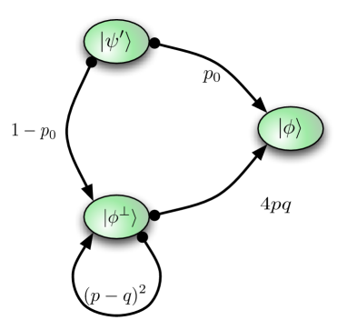
Lemma IV.1.
We can transform any state in the subspace spanned by and into with a procedure using reflections around the states on average. For , define by the equation . We then have .
Proof.
The procedure is as described above. Consider the process of Fig. 2. Define to be the number of reflections used after the first step, if the first step resulted in state . We have . If the first step failed, the second step can either succeed or return to . In the first case, we used reflections. In the second case, the expected number of reflections yet to be used is again . This implies the equation . Thus and .
Similarly, we can calculate by solving the equations and . This gives . The last inequality follows because . ∎
According to Lemma IV.1, the number of reflections used satisfies an exponential decay with a fixed base less than provided that is bounded away from both and . In order to obtain a better behaved transformation that only requires to be bounded away from , we use an overlap-suppression trick to modify . We first add an ancilla in the state . Write and . Reflections around and in the extended statespace can be implemented with properly controlled reflections around and . We can therefore transform into using After we are done, we discard the ancilla to extract the desired state . The overlap-suppression trick leads to the following lemma:
Lemma IV.2.
If , we can transform into with a procedure whose average number of reflections satisfies . For , we have .
Proof.
With the technique just described, the overlap probability is changed from to . Given the assumed lower bound, this ranges from to . Here, . From Lemma IV.1, the average number of reflections used is at most .
To prove the bound on , it suffices to show that for , and apply the last inequality of Lemma IV.1. The function is symmetric in and and achieves its maximum of for the allowed values of at . Using the inequality for and , we get
Since , we conclude that . The constraints on and imply that , so . ∎
The constants used for Lemma IV.2 have been chosen for convenience and have not been optimized. Changing the lower bound on or the parameters of the ancilla state when redefining changes the bounds in the lemma but does not affect the complexities to be derived later.
To deal with the problem of low overlap probability , we extend to a procedure with the property that the initial state is transformed if is large enough and unchanged for too small.
Lemma IV.3.
We can implement a procedure that transforms into a combination of states of the form and , where register is if and if . requires one overlap oracle call with a resolution of , a reflection around , and, in the case where the state is transformed into , one instance of with guaranteed to be at least .
Proof.
To implement , we use the overlap oracle once to obtain a combination of with in the span of and . We then use a reflection around to measure . If the state is determined to be or if , we apply . The properties of the overlap oracle and the choice of parameters ensure that this happens only if . It always happens if . ∎
The procedure provides bounds on the overlap at the cost of calling an overlap oracle. As noted in Sect. III, this results in unwanted overhead when accounting for error amplitudes. This can be avoided if one does not seek guaranteed overlap bounds and accepts the possibility that even at high overlap, the transformation may not succeed.
Lemma IV.4.
We can implement a procedure that transforms into a combination of states of the form and , where register is with probability , and the number of reflections around and is bounded by , where and for .
Register ’s contents indicate whether the transformation succeeded.
Proof.
To implement , we apply a -measurement followed by at most two applications of , stopping if is detected in the measurement. If after this, the state is (as indicated by the last measurement), we alternately make - and -measurements until either or is detected. Register is set to if was detected in the last measurement made. The probability that register is is at least the probability that the first three steps of the process of Fig. 2 terminate at , which is (see the proof of Lemma IV.1). We can improve this by noting that conditional on the failure of these steps, the probability of success in the sequence of alternating measurements is . Multiplying by and adding to we get the overall probability of successful preparation of .
The first part of the procedure uses at most five reflections. The probability of failure to produce an acceptable outcome in a given measurement in the second part is . Thus, if the first part fails, the expected number of reflections used in the second part is . Setting to the number of reflections used if the first part fails (event ), we have . To obtain the last statement of the lemma, it suffices to solve this equation. ∎
For later use, we note the following refinement of the lemma:
Corollary IV.5.
When is invoked on state , the distribution of the number of reflections used by and whether succeeds is independent of any previous events. We also have for , where indicates success or failure of .
Proof.
Let and be the events that the first part of fails and or are eventually obtained, respectively. The probability of is . Conditional on , is even, , and we get
Similarly, conditional on , is odd, and . The claim follows because . ∎
For concreteness, we give the following corollary:
Corollary IV.6.
For , transforms into with probability at least . For , the average number of reflections satisfies , and for , where indicates success or failure of .
Proof.
We use the lower bound for the probability of success. The minimum of for is at , and one can check that the value is above . Since , achieves its maximum on at . We show the last bound for , which is sufficient by log-convexity. In this case and, since , Cor. IV.5 gives the bound. ∎
We let be the procedure obtained by combining the overlap-suppression trick with . The procedures , , , and can be implemented in terms of the reflection oracles when the states and are specified to be eigenstates of and with isolated eigenphases known to satisfy and , and with gaps lower bounded by . Here and are assumed to be known, but not and . In this situation, we say that we know -ranges for the eigenvalues. The instances of the reflection oracles used by the procedures are given by and . We choose the third parameter to be as large as possible, because this decreases the complexity of implementing the reflection oracles in terms of the unitary operators. For the rest of this paper, whenever we use one of , and , we assume that the reflections used are based on reflection oracles with the third argument given by a known lower bound on the minimum gap, by default .
We are interested in the situation where the overlap probability is bounded away from , but we do not know a sufficiently small range for the eigenphase of with respect to its defining operator to use the requisite reflection oracle. We show that a sufficiently small eigenphase range can be obtained with low error if we transform many copies of in parallel into , provided is sufficiently large. The statement of the lemma includes an optional projection such that . This is later used in the context of the overlap-suppression trick so the eigenvalue of the modified unitary does not get confused with the original phases (for instance, see Lemma IV.8).
Lemma IV.7.
Suppose that with , and , where is a projector that we can use to control other operations and . Then, using instances of phase estimation oracles , we can implement an isometry with the following property up to an error amplitude of : transforms into a combination of states of the form
| (7) |
where and .
Proof.
Use system label for the ’th copy of . We can modify the phase estimation oracles so that the eigenphase register contains a non-eigenphase if the input state is in the support of . We implement by first using these modified phase estimation oracles independently on each , placing the eigenphase in register . We can express as . By definition, the ’th instance of acts as for some and some instance-specific additional system .
If we make conceptual -measurements, we detect with probability . Thus, with probability at least (Hoeffding’s inequality hoeffding:qc1963a ), of the values in registers are in . Consider this case. Because of the gap condition, other eigenphases are outside . Thus, there is a with the property that more than half of the are in , and we are guaranteed that is within of . Furthermore, any within of is associated with and therefore within of .
We do not make the measurements of the previous paragraph. Instead we reversibly (and unitarily) determine whether an interval containing more than half of the exists. Except for an error amplitude of , the state satisfies the condition, which we now assume. We reversibly compute the number and the median of the in the interval found. As discussed in the previous paragraph, and is within of . We place in register and in register and reverse all classical reversible computations that were required since invoking the phase estimation oracles. Next we reorder systems so that for , the ’th group is in state and for , it is in the state . Here may be different from because of possible correlations with . The states have not changed because the eigenphases encoded in these states have no correlation with .
For the last step of , we reverse the appropriate instance of on each register . In order to do this we need to have computed the reordering permutation into an additional register, which we retain only if we need to reverse this instance of . The desired combination of states has now been obtained. ∎
From the proof of Lemma IV.7, it can be seen that the error is such that the input systems’ state remains in the tensor product of the span of and .
To complete the transformation from to after applying without using an excessive number of reflections when is close to , we can use the overlap-suppression trick.
Lemma IV.8.
Suppose that with given. Then there is a procedure that transforms into a combination of states of the form up to an error amplitude of , where . uses less than instances of and an average of reflections. We have for .
Proof.
We begin by adding ancilla qubits in state . Define and . For the purposes of using , let , where the second factor acts on the ancilla. We apply and, provided , we use (defined in IV.1) on the registers whose state is now indicated to be . The number of instances of applied is less than . The bounds on the number of reflections used follow by Lemmas IV.2 and II.1. ∎
We need a method for transforming states as in Lemma IV.8 that is well-behaved even for small . In order for the method to work we require that the probabilities of eigenphases other than in have a boundedness property. This will ensure that if has a big overlap with an eigenstate of , then this eigenstate is .
Definition IV.9.
We say that is a -dominant eigenphase of in if for every and associated projector onto eigenspaces of with eigenphases in , implies . We refer to as the resolution at which is dominant and take to be zero-dimensional if it is not specified.
performs the transformation in the following steps. The first determines whether it is possible to confidently find a small interval for without changing each of the copies of by much. We then measure each copy so as to project it onto or . We ensure that the probability of recovering a large number of copies of is high. If some are found or if we found that can be determined sufficiently well, we use the recovered copies of to learn a small interval containing and then transform the states. The first step is encapsulated by the next lemma.
Lemma IV.10.
Suppose that is a -dominant eigenphase of in , where is a projector that we can use to control other operations, , and . Let . Then, using instances of phase estimation oracles and reflections around , we can implement an isometry with the following property up to an error amplitude of : transforms into a combination of states of the form
| (8) |
where if , then and ; if , then and ; and otherwise .
Proof.
We use the notation introduced in the proof of Lemma IV.7 and apply instances of to accommodate the special subspace associated with . We look (reversibly) for the first interval , , containing at least of the phases in registers . If no such interval exists, we set the state of to , else we set it to . Any temporary storage required in the reversible classical computation of the content of is erased. We then reverse the instances of used and make -measurements to determine which of the input registers are in state . Finally, we move the registers in this state to the front and set the state of to .
As in the proof of Lemma IV.7, after phase estimation, for some set the state is a combination of products of for and for . There exists such that . Suppose that we conceptually measure the registers before the reversal of the phase estimation oracles. Let be the number of measured phases that are in . Because , . In particular, the measured phases in principle determine the members of . (We can use this for the analysis but not for the procedure.) We consider the three cases , and . First, if , then, from Hoeffding’s inequality applied to , the probability that is at least . Hence, with error amplitude at most , there is a , and register contains before the reversals of the phase estimation oracles. The reversals successfully restore the initial state up to the given error.
Consider next . The probability that is bounded by . We show that the probability of finding a is small. For this purpose, consider the set of such that . For , any measured phase in is associated with an eigenphase in and therefore different from . Because , the dominance condition ensures that such eigenphases occur with probability at most in . To obtain a good bound on the mentioned probability, we consider the ’s according to ’s location in a small partition of . For any , let be the set of eigenvalues of in and the total probability of eigenphases in in . We claim that we can in principle partition such that . First note that because each eigenphase occurs in at most of the . We can construct the greedily. Initialize and set . Then step through . If , add to and proceed to the next . If not, because , either or . If , initialize , update to and proceed to the next . If , set , reset to , update to and proceed to the next . At the end of the procedure, for all . As we observed above, for all , , and the claim follows. Let be the number of measured phases that are in . Because these phases are due to eigenphases in , it follows from Hoeffding’s inequality that with probability at most . If satisfies that , then the measured phases in are associated with . This is because . Probabilistic reasoning can be applied, so we conclude that the probability of is at most . Thus, with an error amplitude of at most , register contains before the phase estimation reversals, and the reversals successfully restore the initial state.
Finally, consider . Because , the probability that is at least . Therefore, except for an error amplitude of at most , and . We now assume this condition. After reversing the phase estimation oracles, the ’th system is in state if and otherwise. Let be the number of observed in the -measurements. The probability of detecting when the state is or is and , respectively. The average value of is , since and . By Hoeffding’s inequality, for fixed , the probability of the event that is bounded by . To determine a bound on the overall probability of , we must use amplitude addition over different . Thus . There are possible , so the worst case sum of the is . Therefore, . We set and use to see that the amplitude for having is bounded by . By amplitude addition, the overall error amplitude is bounded by , since .
To complete the proof, it suffices to determine the maximum error amplitude. The maximum error bound comes from the second case and is given by . ∎
As we noted for the error amplitude in Lemma IV.7, the error in Lemma IV.10 is such that the input systems’ state remains in the tensor product of the span of and .
The last lemma of this section gives the properties of the parallel state transformation procedure that we outlined above.
Lemma IV.11.
Assume that is a -dominant eigenphase of in with . Then there is a procedure that transforms into a combination of and , where , ’s state is if and if , and the error amplitude is bounded by . The procedure uses less than instances of , where , and an average number of reflections bounded by . We have for .
Note that the procedure implicitly provides overlap information. That is, if the transformation succeeds, the overlap satisfies .
Proof.
We use the overlap suppression trick and change each copy of to and define . Let . We apply the procedure of the previous Lemma. If the first output register (system A in Eq. (8)) contains or if the second register (system B in Eq. (8)) has , we continue. Otherwise we set the return register to and stop.
To continue the procedure, we apply (defined in IV.8) to the first registers (that now contain ), omitting the initial overlap-suppressing steps as they have already been done. The specification of and the assumption ensures that the overlap is big enough to apply , which returns . We then apply the appropriate instances of (defined in IV.1) to the remaining registers to transform into . The reflections around implicitly require . To finish we return the registers and .
The error amplitudes associated with the different steps must be added. From the application of we get to which adds at most .
The number of instances of phase estimation oracles used comes from the application of and . The average number of reflections is bounded by the sum of (from applying ), (from applying ), and at most (from using instances of as in Lemma IV.2). The reflections in are from applications of at most instances of . The total number of instances of is bounded by . To get the tail bounds, apply the bounds from Lemmas IV.2 and II.1, with an additional offset of for the first set of reflections. ∎
V State transformations along a path
We consider paths of eigenstates of unitary operators with eigenphases and gaps as defined in the introduction. We assume the ability to apply any and to prepare . If the exact gaps are difficult to obtain, we take the to be known lower bounds on the gaps. We define . The goal is to transform copies of the initial state into the final state . The transformations’ complexities depend on what is known about the overlaps and the eigenphases along the path. They are designed to provide such information if it is not already known, so that future transformations can be performed more efficiently.
Theorem V.1.
Suppose that we know a subsequence of such that , and phases satisfying . We can then transform to with reflections where and for .
Proof.
Given sufficiently large overlaps, the phases can be inferred to sufficient precision during a parallel state transformation. Note that the eigenphase of for can be determined to within by one call to a phase estimation oracle with resolution and input state . We therefore assume that a phase sufficiently close to is known and reflections around can be applied.
Theorem V.2.
Suppose that we know a subsequence of such that with . We can then transform into with an error amplitude of . The transformation requires instances of phase estimation and an average of reflections . Furthermore for . The transformation provides phases satisfying for .
Proof.
The number of underlying calls to phase estimation oracles per copy of produced by the procedure of Thm. V.2 is within a constant factor of that of Thm. V.1 (where phase estimation is used for the implementation of the reflections). The implementations of the oracles in the former case have an additional overhead to achieve the error goal, see Sect. VI.
Theorems V.1 and V.2 suggest that we can obtain state transformations along paths with complexities bounded by the path length. In particular, if the overlap probabilities are bounded above by , the path length is at least . Although it is possible for to be much smaller than the path length due to shortcuts, generically we do not expect this. If the angular rate along the path is defined and constant, , then regularly spaced ensure that the overlap conditions for the theorems above are satisfied and . On the other hand, if many overlaps are close to , could be large compared to . We can eliminate this possibility if we have sufficient information about the overlaps, or after the first transformation by checking overlaps during the transformation, as the next lemma shows.
Lemma V.3.
Let with be given. Consider a procedure for transforming copies of into copies of in steps, where the steps transform from to with . Neither nor the need to be deterministic, but we assume that after has been reached, information required to perform reflections and call overlap oracles for states with is available. We can then modify the procedure so that it outputs a sequence satisfying for all and for so that . To do so requires calls to overlap oracles , explicit reflections on and invocations of with .
The procedures we describe satisfy that the information required to call reflection and overlap oracles is available when needed by the modification in the lemma.
Proof.
The are elements of . We begin by setting . We ensure that at the end of the ’th step () of the modified procedure, the last that has been determined satisfies the invariant . To do so, let be the last member of that has been determined before the ’th step. If , set . Else, after the transformation into copies of has been accomplished, call the overlap oracle on the first copy of . Then use a reflection around to determine whether the state was preserved. If not, or if the overlap oracle returned , set . If the state was not preserved, then call to restore it. This completes the modification of the ’th step and ensures the desired properties for the determined so far and the invariant. The lower bound on the length follows by adding up the lower bounds on the angular distances between successive for . ∎
When the overlaps or the angular rates are unknown, the state transformation requires a recursive procedure to find a sequence of successive states with sufficiently high overlap. We assume that such states can be found, more specifically, we require that there are no jumps of angular distance equal to some given constant or greater. Our recursive state transformations involve binary subdivision of intervals. To transform the state from to , we check whether we can do it directly at a cost of . If not, we recursively transform from to and then from to . We are interested in the total cost of the transformation. For our purposes, the cost is the number of times the unitaries are used. This is determined by the number of times phase-estimation is used either directly or indirectly when applying reflections. The resolution required is typically the gap, and the cost is related to the inverse gap (Sect. III), which can depend on the position along the path. To enable taking this into account we provide general tools for analyzing the complexity of recursive path transformations based on binary subdivision in Appendix B.
We define the symmetric binary interval tree on , , as the set of intervals constructed by starting with and recursively adjoining and to for every in . We also define the cost of as
| (9) |
With the appropriate choice of the cost function , this is the cost of a recursive state transformation procedure, and we show that it depends linearly on length and at worst logarithmically on the ratio of maximum to average angular rates. For simplicity, we use this estimate to state complexity bounds for state transformations where relevant, with the understanding that local-cost-sensitive estimates can be obtained if needed.
Let , and . If , define .
Lemma V.4.
If for , then
| (10) |
The proof is given in Appendix B.
Let and be as defined in Lemma V.4, where by default , and is clear from context if not specified. Note that finiteness of requires that the path has no jumps of angular distance or more.
Theorem V.5.
Suppose that is a -dominant eigenphase of in for all , where . Let , and . Then we can transform into with an error amplitude bounded by with at most instances of phase estimation oracles with precision at least , an average number of reflections bounded by and for .
Proof.
To implement the transformation, we apply of Lemma IV.11 recursively to the intervals of the BIT, terminating at intervals where the transformation succeeds. The lemma guarantees that the transformation succeeds if the angular length of the interval being tried is less than .
To determine the complexity of the transformation, we need to consider a modified tree cost. Let if and otherwise. Define
| (11) |
This accounts for the fact that the shortest intervals in the tree that require action can be associated with arbitrarily short angular lengths. It is their parents whose angular length must be too long for terminating the recursion. With , is an upper bound on the number of intervals for which transformation is attempted. According to Lemma V.4, this is bounded by . The rest follows by multiplying the complexities in Lemma IV.11 by and applying Lemma II.1. For the error amplitude we used amplitude addition. ∎
The next theorem can be applied when little information on overlaps is available, but we know sufficient eigenphase ranges for performing the necessary reflections. For this we need to consider the case where the transformation has probability of success when . In this case, the process of subdividing may continue indefinitely. For , the expected number of intervals considered is finite with an exponentially decreasing tail probability. This follows from the theory of Galton-Watson processes, but in Appendix C we give a statement and proof sufficient for our purposes.
Theorem V.6.
Let . Suppose that we know phases satisfying . We can transform into using reflections, with for .
Proof.
To implement the transformation, we apply to the intervals of the BIT recursively. ( is defined after Cor. IV.6.) The recursion terminates when a transformation succeeds. For the intervals of angular length greater than , Cor. IV.6 characterizes the distribution of the number of reflections used whether or not the transformation succeeds. For intervals of angular length at most , the number of subintervals that need to be tried is characterized by Lemma C.1, where the success probability satisfies . Whether an interval needs to be tried depends only on whether any of the intervals containing it (that is, above it in the BIT) succeeded. Because of Cor. IV.5, Lemma II.2 can be applied. Thus, according to Cor. IV.6, the total number of reflections used in our transforming across satisfies and for . To finish the proof, as was noted in the proof of Thm. V.5, the number of intervals of the BIT whose parents have angular length greater than is bounded by . These intervals form a subtree . Every reflection can be associated with the smallest interval in for whose traversal it was used. The statistics of the number of reflections associated with each such node are bounded by the ones we obtained for intervals of angular length at most . Thus, we can apply Lemma II.1 to complete the proof. ∎
VI Summary of Complexities
The most salient complexities are summarized in Table 1. The bounds apply uniformly for , , and . We also define . In order to obtain the bounds, it is necessary to take into account the error amplitudes contributed by two sources and make sure they do not exceed the error goal of the algorithm. The first is in the implementation of phase estimation and reflection oracles, and the second in our multi-copy transformations. Calls to either oracle in our algorithms require uses of the underlying unitary operator for error amplitude . If the state transformation requires phase estimations or reflections, then we can set to ensure that the total error is bounded by , since error amplitudes are sub-additive. Thus the complexity in terms of uses of the relevant unitary operators is . The additional error in our multi-copy state transfer algorithm is bounded by per state transformation attempt and is given explicitly in Theorems V.2 and V.5. In our algorithms, the number of phase estimation and reflection oracle calls per copy is linearly related to the number of state transformation attempts. The latter determines the total error from this contribution, which is . Thus, for an error goal of we can set . This requires total phase estimation and reflection oracle calls. After accounting for the error in the implementation of these oracle calls, we obtain a complexity per copy of .
| Knowledge assumed | ||||||||
| Overlap | Overlap | Eigenphase | Eigenphase | Cost per copy | Number of copies | Reference | ||
| approx- | lower | ranges? | dominance? | required | ||||
| imations? | bounds? | |||||||
| 1 |
|
|||||||
| Thm. V.2 | ||||||||
| 1 | Thm. V.6 | |||||||
| Thm. V.5 | ||||||||
The formal meaning of the columns in Table 1 for assumed knowledge can be determined from the statements of the referenced lemmas and theorems. Having knowledge of overlap approximations means knowing enough about the to be able to pick such that is large but bounded away from . This ensures that transforming along the is possible and efficient in terms of path length. Knowing overlap lower bounds ensures the former only. When we say that eigenphase ranges are known, we mean that for all , we know an interval (or more generally, a set) containing such that the distance from this interval to every other eigenphase of is at least . This is sufficient for implementing the reflections with low error. The eigenphase dominance condition ensures that we can statistically distinguish the wanted eigenphase when using multiple copies of the states to infer adequate eigenphase ranges. The formal definition for a path is in Thm. V.5 based on Def. IV.9.
Lemma V.3 can be used to preprocess the transformation steps so that the complexity of the first row of Table 1 applies to subsequent transformations. Use of Lemma V.3 requires calls to overlap oracles, where is the number of actual transformation steps used. Thus, the complexity has an additive term of , according to the note after Def. III.4. However, if the recursive subdivision technique is used as in the last two rows of the table, the use of overlap oracles can be avoided.
We have given the key complexities in terms of global quantities that are simple to state. The complexities actually depend on local aspects of the path. In particular, if the gaps are typically large compared to the minimum, sections of the path can be traversed much more quickly. This can be taken into account by a finer complexity analysis, for example by taking advantage of Lemma B.2.
Our analyses apply to paths of non-degenerate eigenstates, but much of it can be extended to paths of eigenspaces as follows. Suppose that the path is characterized by a family of spaces consisting of a union of eigenspaces of whose set of eigenphases have a minimum distance to all eigenphases of states orthogonal to . The multi-copy transformation algorithms used when we have insufficient information about the eigenphases require that is an eigenspace. Reflections around can be implemented with the functional calculus of as noted after Def. III.3. The goal is to transform an arbitrary initial state into some . To generalize our analysis, it is necessary to redefine the path length. Let be the projector onto . We define , where and . Note that having no large jumps in the path implies that the dimension of is non-decreasing. The basic transformation steps are the same, but their analysis requires the observation that the reflections around the subspaces and are a direct sum of reflections on two-dimensional subspaces of the space spanned by and , see Ref. szegedy_quantum_2004 . Within each such subspace, the transformation behaves as expected. The relevant overlaps now depend on the relationship between the reflection axes in the mentioned two-dimensional subspaces.
Acknowledgements.
We thank A. Harrow for discussions regarding the algorithm in the unknown-eigenphase case. This research was supported by the Perimeter Institute for Theoretical Physics, by the Government of Canada through Industry Canada and by the Province of Ontario through the Ministry of Research and Innovation. Contributions to this work by NIST, an agency of the US government, are not subject to copyright laws. This work was supported by the National Science Foundation under grant PHY-0803371 through the Institute for Quantum Information at the California Institute of Technology. We also thank the Laboratory Directed Research and Development Program at Los Alamos National Laboratory for support.Appendix A Proof of Lemma II.2
Let be the measure for the probability distribution of its arguments. The conditional independence assumption is equivalent to having the and generated via the sequence of probabilistic transitions . It follows that is conditionally independent of the for given . Formally we have
where the omitted identities involve applying the first steps recursively to the last term.
Given the constraints on , we obtain
because is a function of . To get the desired bound, we let , use the monotone convergence theorem, and apply the bound on with :
Appendix B Recursive transformations complexity
Let be the length of the path from to . Define and . We have and the state is constant on the open interval . The functions and are monotone. Given and a distance scale , we define a local maximum speed variation at by
| (12) |
If the set under the supremum is empty, let . To justify the description of as a speed variation, we define average speeds between and by and , allowing for constant sections on the path. A more direct local speed variation is
| (13) |
If the set under the supremum is empty, let . The description of as a speed variation at at scale comes from the observation that
Lemma B.1.
For all intervals
| (14) |
with equality if , the path is continuous and has no constant intervals.
Proof.
The set in the definition of is empty iff or . If the latter holds, then the set in the definition of is empty. If not, then either is empty or . In this case with . Consider , with as in Eq. 12. Let and define , and choose , such that , . Then
For the reverse inequality, given arbitrarily small, choose such that . The constraint on implies that , so . Let be arbitrarily small. Let for and for . Continuity implies that . If , then and we let . Else and we let . Unassigned are set to . The assumptions imply that for small enough, the satisfy the constraints in Eq. 12, showing that . Letting gives the desired result. ∎
The next lemma gives a bound on the cost of a symmetric binary interval tree that is sensitive to local variations.
Lemma B.2.
If for , then
where .
Proof.
The bound is obtained in three steps. First we separately sum over intervals in the tree in each length class . Second, we uniformly, randomly assign the cost to the open interval between and and integrate over the length variable. Third, we use bounds on costs and numbers of intervals in the tree spanning the value of the length variable. The steps are implemented in the following sequence of identities and inequalities:
To finish the proof, note that the number in parenthesis in the last line,
is the size of a set of nested intervals in the tree. Let be the biggest and the smallest of these intervals. Because of the way the tree is constructed, the number of these intervals is given by
where the inequality follows from the definition of . ∎
Finally, we give the proof of Lemma V.4 stated in the text.
Proof of Lemma V.4.
We begin by bounding for in terms of the maximum and average angular rates. If , then so the integral is . Assume and let be arbitrarily small. For every , choose such that the following hold: The satisfy the constraints given in the definition of (see Eq. 12), , and the are measurable functions. We can now bound
Jensen’s inequality, applied to the concave function, gives
We bound the denominator inside the integral with the inequality , which does not depend on the variable of integration, so we can continue by bounding the integral of the numerator. We first change the order of integration
If , then . Similarly, . It follows that the inner integral is bounded by . This gives the bound
Combining the bounds and letting go to , we obtain
Substituting into the bound of Lemma B.2, we get
as desired. ∎
Appendix C A Galton-Watson lemma
Lemma C.1.
Consider the random process starting from which is defined recursively as follows: For all in , replace with with and with probability add and to . Let be the possibly infinite set obtained by running this process countably many times. For , the expected size of is and for .
Proof.
We outline the proof, omitting some necessary existence arguments. Either , which happens with probability , or , where and are independent with the same statistics as . The latter happens with probability . Thus , or . Similarly, using the independence of and again, we find . This is solved by
The relevant solution is the negative branch, as can be seen by checking that . The maximum value of for which it is defined is . For this , . The following sequence of inequalities together with log-convexity completes the proof:
at the maximum . ∎
Appendix D Angular rate estimation
Here are some tools for estimating average angular rates for paths of eigenstates of normal operators.
Lemma D.1.
Let be a normal operator with eigenstate having eigenvalue . Suppose is normal and has an eigenspace with eigenvalue gapped by . Then the maximum angle from to is bounded by .
Proof.
Let be the projector onto the orthogonal complement of . It suffices to show that for all . We can use the “resolvent trick” to express
where the integral is over a circle of radius less than around . Thus
The result follows by letting go to . ∎
Corollary D.2.
Let be a family of normal operators, with all objects differentiable at . Let . If the eigenvalues are gapped with gap in a neighborhood of , then
| (20) |
Proof.
It suffices to apply first-order perturbation theory to Lemma D.1, noting that and . ∎
References
- [1] D. Aharonov and A. Ta-Shma. Adiabatic quantum state generation and statistical zero knowledge. Proceedings of the 35th Annual ACM STOC, pages 20–29, 2003.
- [2] P. Amara, D. Hsu, and J. E. Straub. Global energy minimum searches using an approximate solution of the imaginary time schroedinger equation. The J. of Phys. Chem., 97:6715–6721, 1993.
- [3] A. Ambainis and O. Regev. An elementary proof of the quantum adiabatic theorem. arXiv:quant-ph/0411152, 2004.
- [4] M. H. S. Amin. Consistency of the adiabatic theorem. Phys. Rev. Lett., 102(22):220401–4, 2009.
- [5] A. Aspuru-Guzik, A. D. Dutoi, P. J. Love, and M. Head-Gordon. Simulated quantum computation of molecular energies. Science, 309:1704–1707, 2005.
- [6] J. E. Avron, R. Seiler, and L. G. Yaffe. Adiabatic theorems and applications to the quantum hall effect. Commun. Math. Phys., 110(1):33–49, 1987.
- [7] S. Boixo, E. Knill, and R. D. Somma. Eigenpath traversal by phase randomization. Quantum Inf. and Comp., 9:833–855, 2009.
- [8] S. Boixo and R. D. Somma. Necessary condition for the quantum adiabatic approximation. Phys. Rev. A, 81(3):032308, 2010.
- [9] A. M. Childs, E. Deotto, E. Farhi, J. Goldstone, S. Gutmann, and A. J. Landahl. Quantum search by measurement. Phys. Rev. A, 66:032314, 2002.
- [10] E. Farhi, J. Goldstone, S. Gutmann, J. Lapan, A. Lundgren, and D. Preda. A quantum adiabatic evolution algorithm applied to random instances of an NP-complete problem. Science, 292:472–476, 2001.
- [11] E. Farhi, J. Goldstone, S. Gutmann, and M. Sipser. Quantum computation by adiabatic evolution. arXiv:quant-ph/0001106, 2000.
- [12] A. B. Finnila, M. A. Gomez, C. Sebenik, C. Stenson, and J. D. Doll. Quantum annealing: A new method for minimizing multidimensional functions. Chem. Phys. Lett., 219:343–348, 1994.
- [13] G. A. Hagedorn and A. Joye. Elementary exponential error estimates for the adiabatic approximation. J. Math. Anal. Appl., 267(1):235–246, 2002.
- [14] A. W. Harrow, A. Hassidim, and S. Lloyd. Quantum algorithm for solving linear systems of equations. arXiv:0811.3171, 2008.
- [15] W. Hoeffding. Probability inequalities for sums of bounded random variables. J. Am. Stat. Assoc., 58:13–30, 1963.
- [16] S. Jansen, M-B Ruskai, and R. Seiler. Bounds for the adiabatic approximation with applications to quantum computation. J. Math. Phys., 48(10):102111–15, 2007.
- [17] T. Kadowaki and H. Nishimori. Quantum annealing in the transverse ising model. Phys. Rev. E, 58:5355–5363, 1998.
- [18] E. Knill, G. Ortiz, and R. Somma. Optimal quantum measurements of expectation values of observables. Phys. Rev. A, 75:012328, 2007.
- [19] M. Lewenstein, A. Sanpera, V. Ahufinger, B. Damski, A. Sende, and U. Sen. Ultracold atomic gases in optical lattices: Mimicking condensed matter physics and beyond. Adv. in Phys., 56:243–379, 2007.
- [20] D. A Lidar, A. T Rezakhani, and A. Hamma. Adiabatic approximation with better than exponential accuracy for many-body systems and quantum computation. J. Math. Phys., page 102106, 2009.
- [21] C. Marriott and J. Watrous. Quantum Arthur–-Merlin games. Computational Complexity, 14(2):122–152, 2005.
- [22] D. Nagaj, P. Wocjan, and Y. Zhang. Fast amplification of QMA. Quant. Inf. Comp., 9:1053, 2009.
- [23] O. Oreshkov and J. Calsamiglia. Adiabatic markovian dynamics. arXiv:1002.2219, 2010.
- [24] G. Ortiz, J. E. Gubernatis, E. Knill, and R. Laflamme. Quantum algorithms for fermionic simulations. Phys. Rev. A, 64:022319/1–14, 2001.
- [25] R. D. Somma, S. Boixo, H. Barnum, and E. Knill. Quantum simulations of classical annealing processes. Phys. Rev. Lett., 101:130504–4, 2008.
- [26] M. Szegedy. Quantum speed-up of markov chain based algorithms. Foundations of Computer Science, 2004. Proceedings. 45th Annual IEEE Symposium on, pages 32–41, 2004.
- [27] T. Tulsi, L. Grover, and A. Patel. A new algorith for fixed point quantum search. Quant. Inf. Comp., 6:483, 2006.
- [28] P. Wocjan and A. Abeyesinghe. Speedup via quantum sampling. Phys. Rev. A, 78(4):042336, 2008.
