Characteristics of solar meridional flows during solar cycle 23

Abstract

We have analyzed available full-disc data from the Michelson Doppler Imager (MDI) on board SoHO using the “ring diagram” technique to determine the behavior of solar meridional flows over solar cycle 23 in the outer 2% of the solar radius. We find that the dominant component of meridional flows during solar maximum was much lower than that during the minima at the beginning of cycles 23 and 24. There were differences in the flow velocities even between the two minima. The meridional flows show a migrating pattern with higher-velocity flows migrating towards the equator as activity increases. Additionally, we find that the migrating pattern of the meridional flow matches those of sunspot butterfly diagram and the zonal flows in the shallow layers. A high latitude band in meridional flow appears around 2004, well before the current activity minimum. A Legendre polynomial decomposition of the meridional flows shows that the latitudinal pattern of the flow was also different during the maximum as compared to that during the two minima. The different components of the flow have different time-dependences, and the dependence is different at different depths.

1 Introduction

Meridional flow plays a key role in the operation of solar dynamo. Even as early as the 1970s, these flows were recognized as important in explaining the solar dynamo and differential rotation (e.g., Durney 1975; Bogart & Gierasch 1979). It is believed to be responsible for transporting magnetic elements towards the poles (Wang et al. 1989). It also plays a role in generation of differential rotation and its temporal variations (Glatzmaier & Gilman 1982; Spruit 2003). The meridional flows are also invoked as a means to transport flux towards the equator near the base of the convection zone in some solar dynamo models (e.g., Choudhuri et al. 1995; Dikpati & Charbonneau 1999). There are no measurements of the meridional flow in the deeper layers of the Sun and hence, near-surface measurements, along with other assumptions, can be used to constrain solar dynamo theories.

There is a rich history of the study of the meridional component of flows on the solar surface. (e.g., Schröter & Wöhl 1975; Howard 1979; Topka et al. 1982; Ribes et al. 1985). However, because the meridional-flow speed (about 20 m s^-1) is more than an order of magnitude smaller than other flows at the solar surface, the early observations did not give a clear picture of these flows. Thanks to the improvements in observational techniques, the meridional flow has been reliably measured at the solar surface using both magnetic elements as tracers (Komm et al. 1993; Hathaway & Rightmire 2010) and Doppler velocities (e.g., Hathaway 1996). These observations show a general flow towards the poles in both hemispheres that is roughly antisymmetric about the equator.

The development of local helioseismic techniques enabled the study of meridional flow inside the Sun. Using the time-distance technique Giles et al. (1997) showed that meridional flow persists in the subsurface layers. Schou & Bogart (1998), Basu et al. (1999), Haber et al. (2000) and others applied the ring diagram technique to study the meridional flow in the subsurface layers up to a depth of about 15 Mm below the surface. The local helioseismic techniques used in these studies do not give any information about the deeper layers. In particular, these could not study the layers close to the base of the solar convection zone which is believed to be the region of the return flow from the poles to the equator. On the other hand, global modes that can give information about deeper layers are rather insensitive to meridional flow (Roth & Stix 2008; Chatterjee & Antia 2009) and hence are not useful for this purpose. Nevertheless, even the behavior of meridional flow in the immediate sub-surface layers can give useful information to constrain dynamo models. Some models of zonal flows (Spruit 2003) predict a steep variation with depth in the meridional flow near the surface and hence these models too can be tested with the available seismic data.

The availability of seismic data over a full solar cycle has made it also possible to study the time variations of the meridional flows. There have been such studies with data that cover only a part of the solar cycle (Chou & Dai 2001; Haber et al. 2002; Basu & Antia 2003; González Hernández et al. 2006, 2008, 2010; Zaatri et al. 2006; etc.). All these studies have found significant temporal variations in the meridional flows, though they are not always in complete agreement with each other (see Antia & Basu 2007). Among the results that stand out is that the meridional flow speed is slower at maximum activity than at the minimum (Chou & Dai 2001; subsequently confirmed by Hathaway & Rightmire 2010). Additionally the pattern of the meridional flow also shows bands of fast or slow flows similar to well known zonal flows (Beck et al. 2002; González Hernández et al. 2010).

In this work we use data from the Michelson Doppler Imager (MDI) on board SoHO to study how the sub-surface meridional flows changed over solar cycle 23. We use the ring diagram technique to study the temporal, latitudinal and depth variations in meridional flow. We chose to use MDI data since it samples the entire solar cycle and hence, may give a clear picture of the temporal variations. It may be noted that although MDI instrument has been functioning through the entire cycle 23, except for a short break around 1998, the ring diagram data are available only during the so-called “dynamics runs”, which typically cover only 2-3 months every year, earlier during the cycle and for shorter periods since 2003 when SoHo’s high-gain antenna started malfunctioning. Thus although the entire solar cycle is sampled by the ring diagram data, the coverage is not continuous and the fill factor is rather low. Data from the Global Oscillation Network Group (GONG) are available for the declining phase of cycle 23 only. These have been analyzed by González Hernández et al. (2010). GONG data has the advantage of continuous coverage in time from July 2001 onwards. MDI magnetic field data have been used by Hathaway & Rightmire (2010) to study surface meridional flows.

2 Data

The basic data set consists of ‘ring diagrams’ obtained from full-disk Dopplergrams from the MDI instrument. Ring diagrams (Hill 1988) are three-dimensional (3D) power spectra of short-wavelength modes in a small region of the Sun. High-degree (short-wavelength) modes can be approximated as plane waves over a small area of the Sun as long as the horizontal wavelength of the modes is much smaller than the solar radius. Ring diagrams are obtained from a time series of Dopplergrams of a specific area of the Sun tracked at the mean rotation velocity. A detailed description of the ring diagram technique is given by Patrón et al. (1997), Basu et al. (1999) and Antia & Basu (2007). Ring diagram analysis has the advantage that, unlike global-mode analysis, it can be used to study the horizontal components of solar flows as a function of latitude, longitude, depth and time. In the present work, we average the spectra over longitudes and study the variation of meridional flow as a function of latitude, depth and time.

We use publicly available MDI ring diagrams for this work. Each ring diagram was obtained from a time series of 1664 images covering 16^∘ in longitude and latitude. These square regions are then apodized to circular regions of diameter $15^{\circ}$. Successive spectra are separated by 15^∘ in heliographic longitude of the central meridian. These data are available for fifteen latitudes from 52.5^∘S to 52.5^∘N in steps of 7.5^∘. Wherever possible, we have averaged power spectra for each latitude over one full Carrington rotation. This has not always been possible since MDI operates in the dynamics mode only for a small fraction of the time. These incomplete sets were chosen to get a reasonable sampling of the different phases of cycle 23. Averaging over a number of spectra improves the statistics and reduces the error estimates in the inferred velocity components. Characteristics of the sets used are listed in Table 1. Also listed in the table is the 10.7 cm radio flux as an indicator of the solar activity over the period covered by the data. The 10.7 cm radio flux is obtained from the NOAA, National Geophysical Data Center. Results obtained from some of these data sets had been presented by Basu & Antia (2003), however, we reanalyzed those sets in order to be consistent in our analysis.

Each ring diagram is fitted with the model described by Basu & Antia (1999). The parameter that describes the frequency shift due to meridional flow was then inverted using the methods of Optimally Localized Averages (OLA) and Regularized Least Squares (RLS) to determine the variation of meridional velocity with depth. The inversion results are generally reliable in the depth range of about 1 to 14 Mm ($r=0.98R_{\odot}$ to $0.999R_{\odot}$) as seen by the averaging kernels (Antia & Basu 2007), and the match between OLA and RLS results.

3 Results

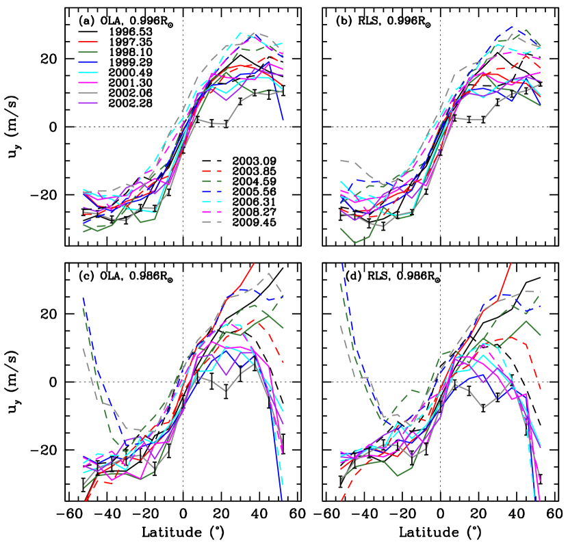
Figure 1: The solar meridional flow velocities as obtained from the both OLA and RLS inversions at depths of 2.8 Mm ($r=0.996R_{\odot}$) and 9.8 Mm ($r=0.986R_{\odot}$) are plotted as a function of latitude. The curves are labeled by the central time for each data set. Positive values indicate northward velocities and negative indicate southward velocities. For the sake of clarity, error bars are plotted on only one curve.

The meridional flow velocities at depths of 2.8 Mm ($r=0.996R_{\odot}$) and 9.8 Mm ($r=0.986R_{\odot}$) obtained from our analysis are shown in Figure 1. We show both OLA and RLS results. Note that both results are by and large similar, giving added confidence in the results. In some cases (e.g., 2009.45 at $r=0.996R_{\odot}$) there are some differences between RLS and OLA results at high latitudes, but these are still within about $3\sigma$ of each other. Considering the large number of results shown in the figure a few differences of this order are to be expected. Furthermore, most of the large differences are at high latitudes where projection effects become important. This effect is not included in the errorbars which in turn results in an underestimation of errors at high latitudes. Thus in real terms, the significance of the differences are even less than what they appear to be from Figure 1. There is a clear temporal variation in the meridional flow velocities. While the dominant flow is from the equator towards the poles in both hemispheres, in some cases there appears to be a flow across the equator. Such flows can be an artifact of position-angle errors (see e.g., Giles et al. 1997), and hence, we ignore these in our analysis and concentrate only on the component that is antisymmetric about the solar equator. The antisymmetric component is obtained by taking an average over both hemispheres, with sign of velocities in the south hemisphere reversed, i.e. $(u_{N}-u_{S})/2$.

The north-south antisymmetric component of the meridional flow at four different depths is shown in Figure 2. Note that the behavior is different at different depths and at different epochs. The flow velocities appear to be the lowest at the shallowest depth that we could probe. However, it is not clear if the flow speed increases below a depth of 4.2 Mm ($r=0.994R_{\odot}$).

The time and latitudinal dependences of the flows is seen more clearly in Figure 3. To give a symmetric appearance we have flipped the sign of flow velocities in the southern hemisphere. It is clear from the figure that the latitudinal dependence of the flows is a function of time and is different at different depths. In particular, in the shallower layers one can see clearly that the flow velocities were smallest when the Sun was most active. As activity during cycle 23 rose, the flows in the higher latitudes started to slow down first and the behavior very quickly migrated to the lower latitudes. The increase in flow-speed with decreasing levels of activity is seen first in the high-latitude regions. This gain in speed is subsequently seen at lower and lower latitudes. Furthermore, the general level of the meridional flow speed in the shallow layers is larger during the current minimum as compared to that during the previous minimum. The behavior is much more complicated in the deeper layers that we can probe reliably, though the general pattern of the higher latitudes reacting first appears to hold.

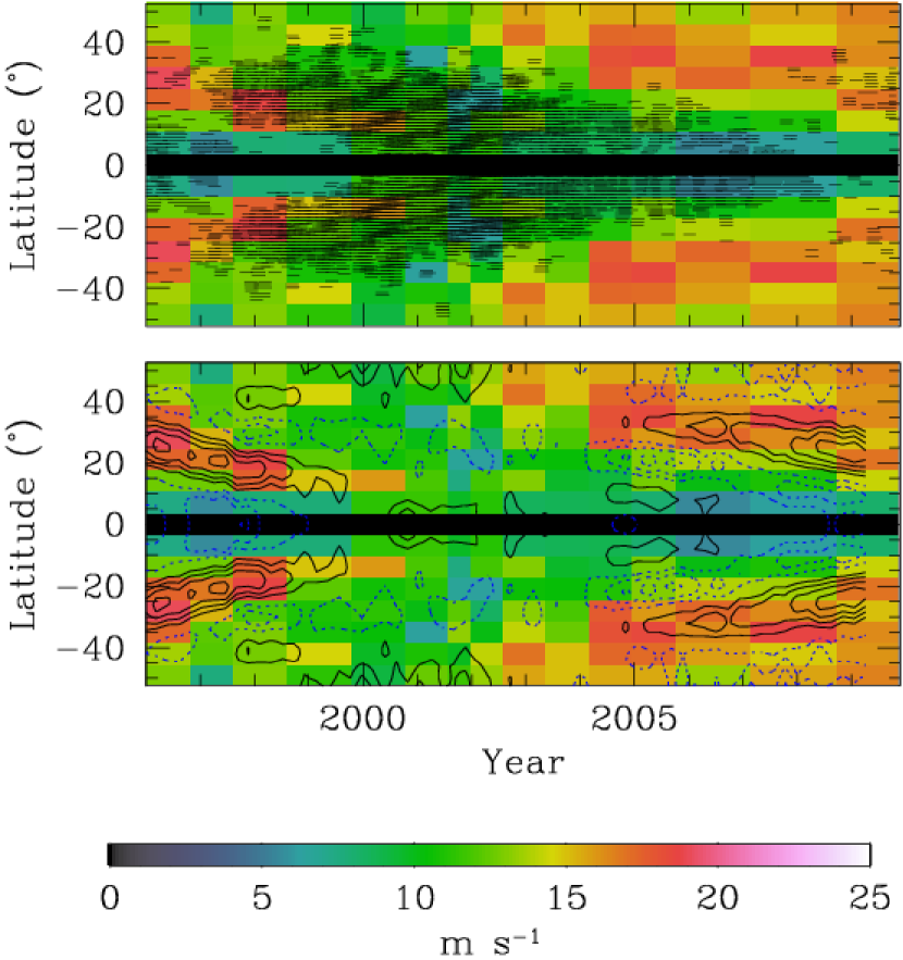
Figure 4: The antisymmetric component of meridional flow plotted as a function of time and latitude at a depth of 1.4 Mm ($r=0.998R_{\odot}$) (cf., Fig. 3) over-plotted with the position of sunspots (upper panel) and contours showing zonal flow velocities (lower panel). The solid contours are for prograde velocities, dashed for retrograde. In the lower panel contours are spaced at intervals of 1m s^-1 and the zero-velocity contour has not been plotted.

The migration of the meridional flows is very similar to the butterfly diagram, as can be seen from Figure 4, where we have over-plotted the position of sunspots during cycle 23 on the meridional flow pattern. As can be seen, there is a good match between the positions of the sunspots and the region of low-speed meridional flows. The concordance is not perfect, but that could be a result of the poor time and latitude resolution of the meridional flow data. Figure 4 also shows the solar zonal flow velocities at the same depth over-plotted on the meridional flows. Again there is a match between the migrating pattern of the meridional flow with that of the zonal flow. The zonal flow velocities were obtained using MDI global mode data (Antia et al. 2008). The bands of high meridional flows coincides with those of high zonal flows. A high speed branch, presumably corresponding to the next solar cycle has started at high latitudes around 2004, well before the current minimum.

To study the detailed behavior of the meridional flows, we obtain a polynomial decomposition of the flow in the manner described by Hathaway (1996)

$$u_{y}(r,\theta,t)=-\sum_{i}C_{i}(r,t)P^{1}_{i}(\cos\theta),$$ (1)

where $P^{1}_{i}$ are associated Legendre polynomials of degree $i$ and order 1, and $\theta$ is the angle from the north pole. We used the standard normalization for the $P^{1}_{i}(\cos\theta)$. Durney (1993) had suggested the presence of components beyond $i=2$. It should be noted that Hathaway (1996) was using only surface Doppler measurements and hence, the expansion-coefficients did not include any $r$ dependence. In Eq. (1), and all our figures, positive $u_{y}(r,\theta,t)$ is the flow towards the solar north pole. In this expansion, the odd-degree coefficients represent the symmetric component of the flows and we ignore those in this work, while the even-degree polynomials are the antisymmetric component, and those are what we concentrate on.

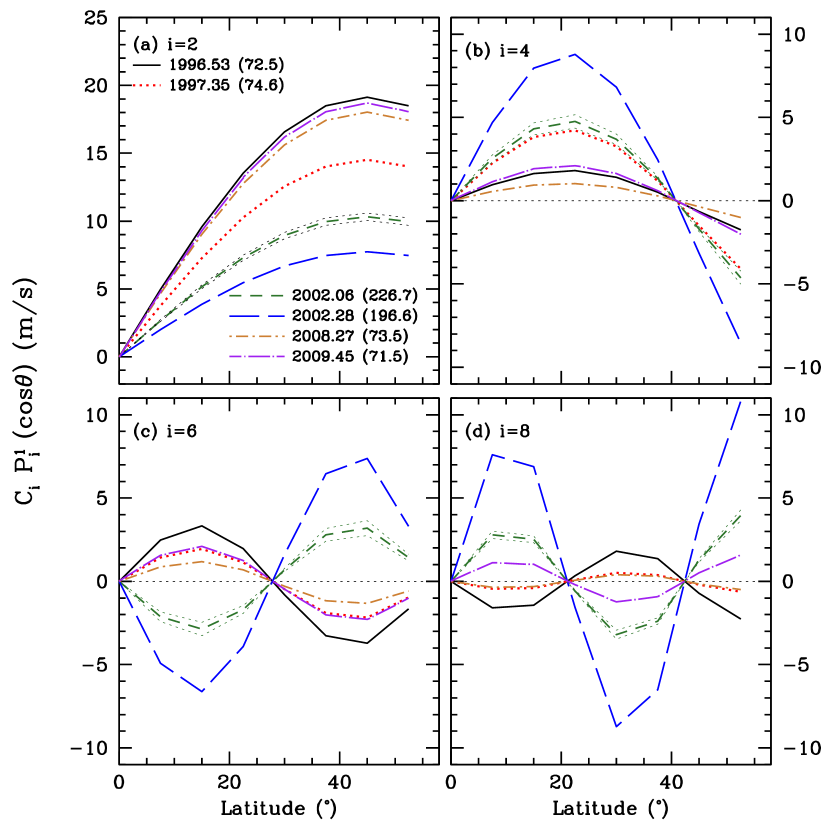
Figure 5: The first 4 antisymmetric Legendre components (see Eq. 1) of the meridional flow at a depth of 1.4 Mm ($r=0.998R_{\odot}$) plotted as a function of latitude. We have plotted results of only six sets to highlight the difference in the flows between solar minimum and maximum and the differences between the minimum before cycle 23 and that before cycle 24. $1\sigma$ error limits are shown for one epoch, the errors are similar for the others. The six sets are labeled by the central time for each data set. The numbers in brackets in the legend indicate the 10.7 cm flux in SFUs.

Figure 5 shows the first four even-degree Legendre components for six epochs — two for the beginning of cycle 23, two near the maximum and two at the beginning of cycle 24. We plot the components for the flow at a depth of 1.4 Mm ($r=0.998R_{\odot}$). Two features stand out from the figures: first, the flow at solar maximum is not merely slower than the flows at solar minimum, they also have different latitudinal dependencies; and second, the flows at the beginning of cycle 24 are different from the flows at the beginning of cycle 23 for comparable levels of global solar activity. The speed of the dominant Legendre component ($i=2$) of the flows shows that the meridional flow was slower at the maximum than at the minimum, though the behavior is by no means monotonic with activity. Perhaps the more interesting component is $i=6$, where there is a clear sign reversal of the flows between minimum and maximum activity. It is also clear that the higher order components make a significant contribution to the flow.

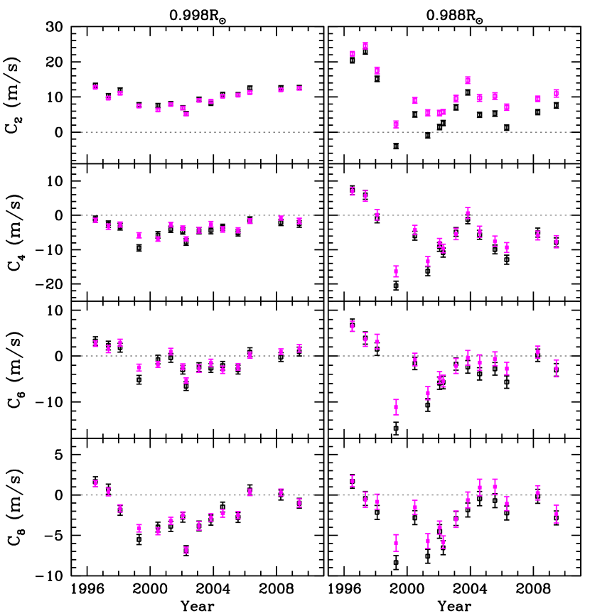
Figure 6: Coefficients of the Legendre decomposition plotted as a function of time for two depths. The black points are RLS results, the magenta (gray in the print version) are OLA results. Note that the pattern of time dependence is different for different coefficients and also for different radii.

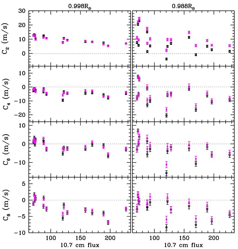
Figure 8: The same as Figure 6, but plotted as a function of the 10.7 cm radio flux expressed in solar flux units.

The behavior of the coefficients at two different depths is plotted as a function of time in Figure 6 and the behavior as a function of depth for six different epochs is plotted in Figure 7. It is clear from the figures that (a) the coefficients changed with time, (b) different coefficients had different time-dependences, (c) that the coefficients were very different during the solar maximum as compared to those at the two minima, and (d) coefficients at different depths show different time dependence. Since each component has a different temporal and depth dependence, the resulting pattern shows a more complex behavior. The same data are plotted as a function of the global solar activity index (the 10.7 cm radio flux) in Figure 8. There appears to be a reasonable correlation (rather an anti-correlation) between the $C_{2}$ coefficient and activity index at a depth of 1.4 Mm ($r=0.998R_{\odot}$), the correlation is less strong for the higher-order coefficients. The pattern is however, much more confused in the deeper layers. While the $C_{2}$ coefficient is almost flat, the higher-order coefficients show two branches. The rising phase of cycle 23 appears to populate the lower branch, while the declining phase and the cycle 24 minimum populates the upper, almost flat branch.

An alternative representation of the meridional flows can be obtained by assuming that the flow is periodic with the period of the solar cycle. Under this assumption we can expand the flow as:

$$u_{y}(r,\theta,t)=u_{a}(r,\theta)+u_{1}(r,\theta)\sin(\omega t)+u_{2}(r,\theta)\cos(\omega t),$$ (2)

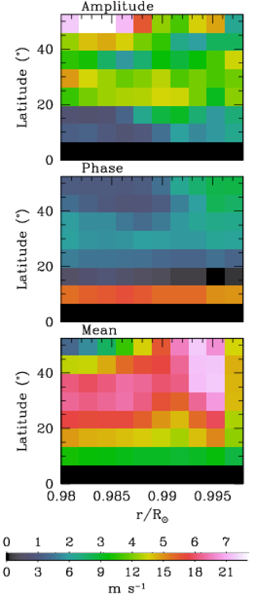
Figure 9: The (temporal) mean meridional velocity as well as the amplitude and phase of the oscillatory part of the meridional flows (see Eq. 2) are shown as a function of depth and latitude. The lower scale on the color bar refer to the mean velocity, while the upper one refers to the amplitude (in m s^-1) and phase of the oscillatory component.

where $\omega=2\pi/T$ is the frequency of the solar cycle. We have used $T=11.8$ years, which is the value we obtain from solar zonal flow studies. The coefficients $u_{a},u_{1},u_{2}$ are calculated at each value of $r$ for each $\theta$. The last two coefficients thus give the amplitude and the phase of the time-varying component. The results are shown in Figure 9. Since we only consider the antisymmetric component of the flow, only results for the northern hemisphere are shown. It can be seen that the time-averaged flow speed, $u_{a}$, is maximum at intermediate latitudes. This mean velocity is small at the outermost layer considered in this work, i.e., a depth of 1.4 Mm ($r=0.998R_{\odot}$), but increases steeply with depth, and appears to decrease marginally in deeper layers. The amplitude of the oscillatory part increases with latitude, while the phase appears to show a complicated behavior. At the latitude of $7.5^{\circ}$ the phase appears to be very large, but that is because we have constrained the value of the phase to be between 0 and $2\pi$. Alternately, we can interpret the phase to be marginally negative at this latitude. It then becomes positive and increases with latitude. Given that we are only showing the antisymmetric component, 7.5^∘ is the lowest latitude for which we have data.

4 Discussion

We have studied solar meridional flows and their variations from June 1996 to April 2009 using the ring diagram technique applied to full-disc Dopplergrams from MDI. This period covers the solar cycle 23 in its entirety. The striking feature that we find is that the flows not only vary with depth, and latitude, but that the time-dependence of the variation is a function of both depth and latitude.

The meridional flows show a migrating pattern, very similar to that of the zonal flows. This result was first seen in time-distance measurements of Beck et al. (2002) and they had concluded that there is a strong correlation between the time-dependent part of the meridional flows and the torsional oscillations (zonal flows). This was later confirmed using GONG data by González Hernández et al. (2010). However, Beck et al. (2002) only had data for the rising part of the cycle, while González Hernández et al. (2010), using GONG data, could only study the declining phase of cycle 23. As a result, it was not completely clear whether the meridional flow pattern matches the zonal flow bands. Our results confirm the migrating pattern, and also that close to the surface the migration mimics the migration of the zonal flows. We find that a band of faster flow at high latitudes has appeared around 2004, long before the current minimum, this is also seen with GONG data (González Hernández et al. 2010). However, we find that although the pattern of the zonal flow is similar from the surface down to a radius of $0.90R_{\odot}$ (e.g. Antia et al. 2008), the meridional flow pattern changes rapidly with depth. It is possible that flow pattern at the deeper levels reflects the magnetic field pattern at those levels, however, the question then would be the lack of the change in the zonal flows. It is, however, not completely clear if the differences in the depth-dependence of the zonal and meridional flow patterns is of a fundamental nature, or simply a results of the fact that ring diagram results have a higher radial resolution near the solar surface compared to global mode analyses used to study zonal flows.

Svanda et al. (2008) have studied the effects of solar active regions on meridional flows and claim that a part of the temporal variation at low latitudes could be explained by flows around active regions. This could explain the shifting pattern of the meridional flows, but not all of the observed temporal variation. However, by masking out active regions González Hernández et al. (2008) showed that while the resultant flow velocity that they obtain changes in the process, there is a second component that still shows a decreasing amplitude as magnetic activity increases. Thus what we are seeing is not merely a local effect of sunspot magnetic fields. In addition to sunspots, there is some evidence to suggest that the variation in the B-angle, $B_{0}$. with time also may cause apparent temporal variation in meridional flows (Zaatri et al. 2006). This has been argued to be the reason why some results showed presence of counter cells in layers below the surface (Haber et al. 2002; González Hernández et al. 2006). However, in this work we have used only the antisymmetric component of the meridional flow, which minimizes the effect of $B_{0}$ angle variation. Thus we do not expect our results to be significantly affected by variation in $B_{0}$. The fact that we see a consistent variation in the meridional-flow velocity supports this conclusion.

In order to get a better understanding of the flow pattern, we decompose the latitudinal dependence in terms of associated Legendre polynomials. This decomposition of meridional flows shows that higher degree components also make a significant contribution. These components do not have the same sign at all latitudes in a given hemisphere, and hence, they give rise to a complex pattern of variation in the resulting flows. These components, in particular, the $P^{1}_{6}$ and $P^{1}_{8}$ components, change sign with time and are reversed during the solar maximum with respect to the flow during the solar minimum. While the higher order components show a time-variation, the changes are not clearly correlated to solar activity. This is probably the result of the fact that global activity indices are obtained by averaging over the disc while the higher components of flows have a complex latitudinal dependence.

The dominant component of meridional flow ($P_{2}^{1}(\cos\theta)$) shows a clear variation with time that is anti-correlated with global solar activity. Chou & Dai (2001) also found similar results. Basu & Antia (2003) had also found similar variations but the result was not very clear with the limited data available at that time. The extended minimum before cycle 24 clearly shows up in the variation of coefficient $C_{2}$ in the shallower layers. There is no sign until the last data set (June 2009) of $C_{2}$ starting to decrease. Our results indicate that the magnitude of this component is similar between the two minima of cycles 23 and 24. Our results are qualitatively similar to those found by Hathaway & Rightmire (2010) from magnetic-field observations made by MDI, though the amplitude they find is consistently lower than what we find after correcting for the difference in normalization. We get $C_{2}$ values of $12.8\pm 0.4$ m s^-1, $6.9\pm 0.4$ m s^-1 and $12.5\pm 0.5$ m s^-1 respectively, for mid-1996, early 2002 and mid 2009 at a depth of 1.4 Mm ($r=0.998R_{\odot}$). It should be noted that Hathaway & Rightmire (2010) report the amplitude of the $2\sin\theta\cos\theta$ term while we use $P_{2}^{1}(\cos\theta)=-3\sin\theta\cos\theta$. Thus our $C_{2}$ should be multiplied by 1.5 before comparing with their values. Hathaway & Rightmire (2010) also find the coefficient $C_{2}$ to be larger during the current minimum as compared to that during the previous minimum. We however, do not find a significant difference at the lowest activity levels that we have access to, however $C_{2}$ during slightly higher activity levels (albeit still low activity) are somewhat different during the minimum of cycle 24 compared with those of cycle 23. The differences are clearly seen in the coefficients of the higher order components in Legendre decomposition. As can be seen from Table 1, the activity level during the first set in our list is the same as that during the last set. Unfortunately, we do not have data for December 2008, when solar activity was lowest. It is quite possible that the difference between our results and those of Hathaway & Rightmire (2010) is because we are looking at different depths, or because of the different observables and techniques used in the two studies. Our results show a rapid variation of flow amplitudes with depth and it is not clear what depth is probed by the magnetic features used by Hathaway & Rightmire (2010).

The strength of the solar meridional flow is believed to play an important role in transporting magnetic flux. Devore et al. (1984) show that the meridional flows play a significant role in magnetic field distribution at low activity. A lower meridional flow speed tends to give stronger polar fields (Sheeley et al. 1989). Our results (see Figure 3) would imply a weaker polar field during the minimum of cycle 24. That is indeed the case. Wang et al. (2009) find that the polar fields during the minimum of cycle 24 were about 40% weeker than that during the earlier minimum.

As mentioned earlier, we find that the meridional flow speed increases with depth. The increase in meridional flow amplitudes with depth in the near-surface layers is seen in ad hoc models of the solar meridional flow (e.g., Roth et al. 2002; Chatterjee & Antia 2009). In these models the increase can be attributed to the boundary condition of radial velocity vanishing at the top boundary and the small density scale heights in the subsurface layers. In these models the meridional velocity has a maximum close to the surface, around a depth of 3.5 Mm ($r=0.995R_{\odot}$), and then decreases becoming significantly less below a depth of 14 Mm ($r=0.98R_{\odot}$). Since these features are essentially a result of the continuity equation, similar variations may be seen in more realistic profiles or in the Sun. On the other hand, Spruit (2003) has proposed a model for torsional oscillations as a geostrophic flow due to lower subsurface temperatures in active regions. This model also gives rise to a meridional flow. However, it predicts that the meridional flow amplitude would decrease with depth, which is opposite to what we find. If this trend is confirmed, such models will be ruled out.

Our results are for very shallow layers of the Sun; we can only probe the outer 2% of solar radius with any reliability. There would be considerable scientific return if the analysis could be extended to deeper layers not covered in this work. González Hernández et al (2006) have tried getting results for deeper layers of the Sun using ring diagrams of regions of size 32^∘ (in contrast, this and other ring diagram work use 16^∘ regions) and find they can cover the outer 5% of the Sun. However, this technique has the drawback that it necessarily degrades the latitudinal resolution. Perhaps a combination of rings-diagrams of different sizes is required to get a good coverage. Time-distance helioseismology could, in principle, give us information of flows in the deeper layer, but again there would be a tradeoff in terms of latitudinal resolution. Data from the Helioseismic and Magnetic Imager (HMI) on board the recently launched Solar Dynamics Observatory will undoubtedly provide us with a better picture of solar meridional flows, though analyzing meridional flows in the deeper layers will remain a problem. The data, however, will allow us to study cycle-to-cycle variations of the flows. The higher resolution of HMI will also allow us to extend helioseismic meridional flow studies to higher latitudes.

Table 1: Data sets analyzed

Carrington	Dates	10.7 cm Flux
Rotation		(SFU)1
1910	1996:06:01 – 1996:06:28	$\phantom{0}71.7\pm 0.3$
1922	1997:04:24 – 1997:05:22	$\phantom{0}74.6\pm 0.6$
1932	1998:01:22 – 1998:02:18	$\phantom{0}87.9\pm 1.5$
1948	1999:04:04 – 1999:05:01	$120.4\pm 2.5$
1964	2000:06:13 – 2000:07:10	$188.9\pm 3.8$
1975	2001:04:09 – 2001:05:06	$169.9\pm 4.6$
1985	2002:01:11 – 2002:02:02	$226.7\pm 3.1$
1988	2002:03:30 – 2002:04:26	$196.6\pm 3.1$
1999	2003:01:25 – 2003:02:10	$128.0\pm 2.1$
2009	2003:10:22 – 2003:11:17	$158.4\pm 13.7$
2019	2004:07:22 – 2004:08:18	$122.1\pm 5.2$
2032	2005:07:11 – 2005:08:08	$\phantom{0}92.9\pm 2.4$
2042	2006:04:10 – 2006:05:08	$\phantom{0}88.2\pm 1.6$
2068-69	2008:03:24 – 2008:04:27	$\phantom{0}73.5\pm 0.9$
2083-84	2009:05:20 – 2009:06:16	$\phantom{0}71.5\pm 0.3$

Figure 2: The velocity of the north-south antisymmetric component of the meridional flows plotted for four depths as a function of latitude. Only OLA inversion results are shown, RLS results are very similar. As in Figure 1, error bars are shown only on one curve.

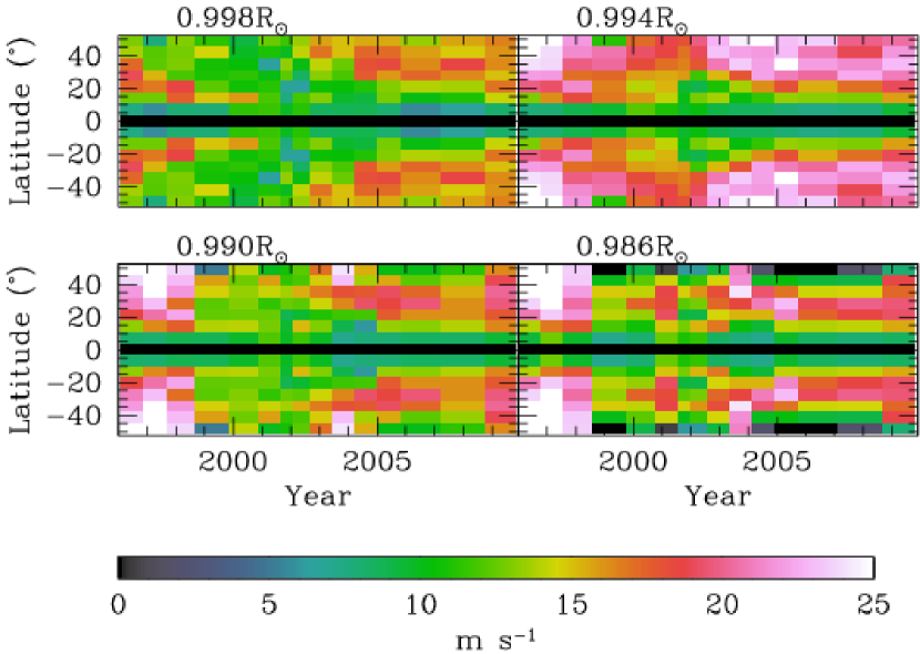
Figure 3: The speed of the antisymmetric component of the meridional flows plotted as a function of latitude and time at four depths. To make the plot symmetric, the sign of flow has been reversed in the southern hemisphere. Thus positive velocity points towards the poles in both hemispheres. Each data point is assumed to represent the time interval between the mid-points with neighboring sets. The actual time covered by each set (which is typically one Carrington rotation) is usually much smaller than the interval between the sets.

Figure 7: Coefficients of the Legendre decomposition plotted as a function of depth for the six epochs plotted in Figure 5. The colors and line-styles in this figure are the same as those in Figure 5. $1\sigma$ error limits are shown only for one epoch, the errors for the others are similar.

References

- Antia & Basu (2007) Antia, H. M., & Basu, S. 2007, AN, 328, 257
- Antia et al. (2008) Antia, H. M., Basu, S., & Chitre, S. M. 2008, ApJ 681, 680
- Basu, Antia & Tripathy (1999) Basu, S., Antia, H. M., & Tripathy, S. 1999, ApJ, 512, 458
- Basu & Antia (1999) Basu, S., & Antia, H. M. 1999, ApJ 525, 517
- Basu & Antia (2003) Basu, S., Antia, & H. M. 2003, ApJ 585, 553
- Beck et al. (2002) Beck, J. G., Gizon, L., & Duvall, T. L., Jr. 2002, ApJ 575, L47
- Bogart & Gierasch (1979) Bogart, R. S., & Gierasch, P. J. 1979, ApJ 228, 624
- Chatterjee & Antia (2009) Chatterjee, P., & Antia, H. M. 2009, ApJ 707, 208
- Chou & Dai (2001) Chou, D.-Y., & Dai, D.-C. 2001, ApJ 559, L175
- Choudhuri et al. (1995) Choudhuri, A. R., Schüssler, M., & Dikpati, M. 1995, A&A, 303, 29
- Devore et al. (1984) Devore, C. R., Boris, J. P., & Sheeley, N. R., Jr. 1984, Solar Physics, 92, 1
- Dikpati & Charbonneau (1999) Dikpati, M., & Charbonneau, P. 1999, ApJ 518, 508
- Durney (1975) Durney, B. R. 1975, ApJ 199, 761
- Durney (1993) Durney, B. R. 1993, ApJ 407, 367
- Giles et al. (1997) Giles, P. M, Duvall, T. L., Jr., Scherrer, P. H., & Bogart, R. S. 1997, Nature 390, 52
- Glatzmaier & Gilman (1982) Glatzmaier, G. A., Gilman, P. A. 1982, ApJ 256, 316
- González Hernández et al. (2006) González Hernández, I., Komm, R., Hill, F., Howe, R., Corbard, T., & Haber, D. A. 2006, ApJ 638, 576
- González Hernández et al. (2008) González Hernández, I., Kholikov, S., Hill, F., Howe, R., & Komm, R. 2008, Sol. Phys. 252, 235
- González Hernández et al. (2010) González Hernández, I., Howe, R., Komm, R., & Hill, F. 2010, ApJ 713, L16
- Haber et al. (2000) Haber, D. A., Hindman, B. W., Toomre, J., Bogart, R. S., Thompson, M. J., & Hill, F. 2000, Solar Phys. 192, 335
- Haber et al. (2002) Haber, D. A., Hindman, B. W., Toomre, J., Bogart, R. S., Larsen, R. M., & Hill, F. 2002, ApJ 570, 855
- Hathaway (1996) Hathaway, D. H. 1996, ApJ, 460, 1027
- Hathaway & Rightmire (2010) Hathaway, D. H., & Rightmire, L. 2010, Science 327, 1350
- Hill (1988) Hill, F. 1988, ApJ 333, 996
- Howard (1979) Howard, R. 1979, ApJ 228, L45
- Komm et al. (1993) Komm, R. W., Howard, R. F. & Harvey, J. W. 1993, Solar Phys., 147, 207
- Patrón et al. (1997) Patrón, J., et al. 1997, ApJ 485, 869
- Ribes et al. (1985) Ribes, E., Mein, P., & Mangeney, A. 1985, Nature 318, 170
- Roth & Stix (2008) Roth, M., & Stix, M. 2008, Solar Phys., 251, 77
- Roth et al. (2002) Roth, M., Howe, R., & Komm, R. 2002, A&A, 396, 243
- Schou & Bogart (1998) Schou, J., & Bogart, R. S. 1998, ApJ 504, L131
- Schröter & Wöhl (1975) Schröter, E H., & Wöhl, H. 1975, Sol. Phys. 42, 3
- Sheeley et al. (1989) Sheeley, N. R., Jr., Wang, Y.-M., & Devore, C. R. 1989, Solar Phys., 124. 1
- Spruit (2003) Spruit, H. C. 2003, Sol. Phys. 213, 1
- Svanda et al. (2008) Svanda, M., Kosovichev, A. G., & Zhao, J. 2008, ApJ 680, L161
- Topka et al. (1982) Topka, K., Moore, R., Labonte, B. J., & Howard, R. 1982, Sol. Phys. 79, 231
- Wang et al. (1989) Wang, Y.-M., Nash, A. G., & Sheeley, N. R., Jr. 1989, Science 245, 712
- Wang et al. (2009) Wang, Y.-M., Robbrecht, E., & Sheeley, N. R., Jr. 2009, ApJ 707, 1372
- Zaatri et al. (2006) Zaatri, A., Komm, R., González Hernández, I., Howe, R., & Corbard, T. 2006, Solar Phys. 236, 227