The VLT LBG Redshift Survey I: Clustering and Dynamics of $\approx 1000$ Galaxies at $z\approx 3$

Abstract

We present the initial imaging and spectroscopic data acquired as part of the VLT VIMOS Lyman-break galaxy Survey. $UBR$ (or $UBVI$) imaging covers five $\approx 36\arcmin\times 36\arcmin$ fields centred on bright $z>3$ QSOs, allowing $\approx 21,000$ $2<z<3.5$ galaxy candidates to be selected using the Lyman-break technique. We performed spectroscopic follow-up using VLT VIMOS, measuring redshifts for 1020 $z>2$ Lyman-break galaxies and 10 $z>2$ QSOs from a total of 19 VIMOS pointings. From the galaxy spectra, we observe a $625\pm 510~{}{\rm kms}^{-1}$ velocity offset between the interstellar absorption and Ly$\alpha$ emission line redshifts, consistent with previous results. Using the photometric and spectroscopic catalogues, we have analysed the galaxy clustering at $z\approx 3$. The angular correlation function, $w(\theta)$, is well fit by a double power-law with clustering scale-length, $r_{0}=3.19^{+0.32}_{-0.54}~{}h^{-1}{\rm Mpc}$ and slope $\gamma=2.45$ for $r<1~{}h^{-1}{\rm Mpc}$ and $r_{0}=4.37^{+0.43}_{-0.55}~{}h^{-1}{\rm Mpc}$ with $\gamma=1.61\pm 0.15$ at larger scales. Using the redshift sample we estimate the semi-projected correlation function, $w_{p}(\sigma)$ and, for a $\gamma=1.8$ power-law, find $r_{0}=3.67^{+0.23}_{-0.24}~{}h^{-1}{\rm Mpc}$ for the VLT sample and $r_{0}=3.98^{+0.14}_{-0.15}~{}h^{-1}{\rm Mpc}$ for a combined VLT$+$Keck sample. From $\xi(s)$ and $\xi(\sigma,\pi)$, and assuming the above $\xi(r)$ models, we find that the combined VLT and Keck surveys require a galaxy pairwise velocity dispersion of $\approx 700~{}{\rm kms}^{-1}$, higher than the $\approx 400~{}{\rm kms}^{-1}$ assumed by previous authors. We also measure a value for the gravitational growth rate parameter of $\beta(z=3)=0.48\pm 0.17$, again higher than previously found and implying a low value for the bias of $b=2.06^{+1.1}_{-0.5}$. This value is consistent with the galaxy clustering amplitude which gives $b=2.22\pm 0.16$, assuming the standard cosmology, implying that the evolution of the gravitational growth rate is also consistent with Einstein gravity. Finally, we have compared our Lyman-break galaxy clustering amplitudes with lower redshift measurements and find that the clustering strength is not inconsistent with that of low-redshift $L^{*}$ spirals for simple ‘long-lived’ galaxy models.

1 Introduction

Observations of the $z\sim 3$ galaxy population present a valuable tool for studying cosmology and galaxy formation and evolution. For cosmology, the interest is in measuring the galaxy clustering amplitudes and redshift space distortions at high redshift. They both lead to virtually independent estimates of the bias whose consistency leads to a test of the standard cosmological model. For theories of galaxy formation and evolution, this is a key period in the history of the Universe in which significant levels of star formation shape both galaxies and the inter-galactic medium (IGM) around them. An especially vital direction of study is the effect of galactic winds at this epoch. Such winds have been directly observed at low (Heckman et al., 1990; Lehnert et al., 1999; Martin, 2005, 2006) and high (Pettini et al., 2001; Adelberger et al., 2003; Wilman et al., 2005; Adelberger et al., 2005a) redshift and are invoked to explain a range of astrophysical phenomena.

A basic item of cosmological interest is the spatial clustering of the $z\approx 3$ galaxy population itself. In $\Lambda$CDM, structure in the Universe is known to grow hierarchically through gravitational instability (e.g. Mo & White 1996; Jenkins et al. 1998; Springel et al. 2006) and testing this model requires the measurement of the clustering of matter in the Universe across cosmic time (e.g. Springel et al. 2005; Orsi et al. 2008; Kim et al. 2009). Surveys of matter at $z\approx 3$ currently focus on two main populations, LBGs and Lyman-$\alpha$ emitters (LAEs). A number of measurements of galaxy clustering are available at $z\approx 3$. For example, Adelberger et al. (2003) and da Ângela et al. (2005a) use the Keck LBG sample with spectroscopic redshfits of Steidel et al. (2003) to measure LBG clustering clustering lengths of $r_{0}=3.96\pm 0.29~{}h^{-1}{\rm Mpc}$ and $r_{0}=4.48^{+0.17}_{-0.18}~{}h^{-1}{\rm Mpc}$ respectively. Further surveys of LBGs at $z\approx 3$ have produced a range of results with, for example, Foucaud et al. (2003) measuring a clustering length for a photometric sample selected from the CFHT Legacy Survey of $r_{0}=5.9\pm 0.5~{}h^{-1}{\rm Mpc}$, Adelberger et al. (2005b) measured $r_{0}=4.0\pm 0.6~{}h^{-1}{\rm Mpc}$ at $\langle z\rangle=2.9$ using a different photometric sample whilst Hildebrandt et al. (2007) measured a value of $r_{0}=4.8\pm 0.3~{}h^{-1}{\rm Mpc}$ from an LBG sample taken from GaBoDS data.

da Ângela et al. (2005a) go on to use the Keck LBG sample to investigate, via redshift space distortions, the gravitational growth rate of the galaxy population at $z\approx 3$, measuring an infall parameter of $\beta(z=3)=0.25^{+0.05}_{-0.06}$. The infall parameter, $\beta$, quantifies the large-scale infall towards density inhomogeneities (Hamilton, 1992; Hawkins et al., 2003) and is defined as $\beta(z)=\Omega_{m}(z)^{0.6}/b(z)$, where $\Omega_{m}(z)$ is the matter density and $b(z)$ is the bias of the galaxy population. The 2dF Galaxy Redshift Survey (2dFGRS) measurement of the infall parameter nearer the present epoch gave $\beta(z\approx 0.1)=0.49\pm 0.09$ (Hawkins et al., 2003), similar to values obtained by previous local measurements (e.g. Ratcliffe et al. 1998). There have also been dynamical measurements of $\beta$ at intermediate redshifts using Luminous Red Galaxies where Ross et al. (2007) found $\beta(z=0.55)=0.4\pm 0.05$. da Ângela et al. (2005b) used the combined 2dF and 2SLAQ QSO redshift surveys to find $\beta(z=1.5)=0.60\pm 0.14$. Finally, Guzzo et al. (2008) used the VVDS galaxy redshift survey to measure $\beta(z=0.77)=0.70\pm 0.26$. As emphasised by Guzzo et al. (2008), if there are independent estimates of $b(z)$ for each redshift sample, then the standard model prediction for the evolution with redshift of the gravitational growth rate of $f=\Omega_{m}(z)^{0.6}$ can be tested against alternative gravity models. Here, we shall follow da Ângela et al. (2005a, b); Hoyle et al. (2002) in making their version of the redshift-space distortion cosmological test which also incorporates the Alcock & Paczynski (1979) geometric cosmological test.

From redshift-space distortions, we can also determine the small-scale dynamics of the galaxy population which are usually simply modelled as a Gaussian velocity dispersion, measured from the length of the ‘fingers-of-God’ (Jackson, 1972; Kaiser, 1987) in redshift space clustering. This velocity dispersion will generally also include the effects of velocity measurement error. Although da Ângela et al. (2005a) had to assume a fixed value of $<w_{z}^{2}>^{1/2}=400~{}{\rm kms}^{-1}$ for the mean pairwise velocity dispersion when making their LBG measurement of $\beta(z=3)$, in bigger surveys it is possble to fit for $<w_{z}^{2}>^{1/2}$ and $\beta$ simultaneously. Thus in 2dFGRS at $z\approx 0.1$, Hawkins et al. (2003) measured a pairwise velocity dispersion of $<w_{z}^{2}>^{1/2}\approx 500~{}{\rm kms}^{-1}$. As well as being of interest cosmologically, the intrinsic galaxy-galaxy velocity dispersion is interesting in terms of establishing the group environment for galaxy formation. Furthermore, these random peculiar velocities dominate at the smallest spatial scales, significantly affecting clustering measurements on scales $r\lesssim 5~{}h^{-1}{\rm Mpc}$. They influence both the observed galaxy-galaxy clustering and the observed correlation between galaxy positions and nearby Ly$\alpha$ forest absorption from the IGM (as measured in Adelberger et al. 2003, 2005a and Crighton et al. 2010). To interpret galaxy-IGM clustering results we shall see that measurements of the small scale dynamical velocity dispersion of the galaxy population are very important.

Galactic winds powered by supernovae are a crucial ingredient in models of galaxy formation (Dekel & Silk, 1986; White & Frenk, 1991). Such negative feedback is required to quench the formation of small galaxies and make the observed faint-end of the galaxy luminosity function much flatter than the low-mass end of the dark-matter mass function, see for example the semi-analytical model of Cole et al. (2000). Simulations without such strong feedback tend to produce galaxies with too massive a bulge, which consequently do not lie on the observed Tully-Fisher relation (Steinmetz & Navarro, 1999; Governato et al., 2010). Such winds can also remove a significant fraction of baryons from the forming galaxy, thereby explaining why galaxies are missing most of their baryons (Bregman et al., 2009), and hence are much fainter in X-ray emission than expected (Crain et al., 2010). In addition, observations of the IGM as probed with QSO sightlines reveal the presence of metals even in the low density regions producing Ly$\alpha$ forest absorption (Songaila & Cowie, 1996; Pettini et al., 2003; Aguirre et al., 2004; Aracil et al., 2004). Other than enrichment from galactic scale winds, it is difficult to see from where these metals originate and this is confirmed by simulations (e.g. Wiersma et al. 2009).

Direct evidence for outflows in high redshift galaxies came from the Keck LBG survey spectra analysed by Adelberger et al. (2003) and Shapley et al. (2003) who found evidence for offsets in the positions of ISM absorption lines, Ly$\alpha$ emission and rest-frame optical emission lines (see also Pettini et al. 2000, 2002). Shapley et al. (2003) present a model in which the optical emission lines arise in nebular star-forming HII regions, giving the intrinsic galaxy redshift, whilst the ISM absorption lines originate from outflowing material surrounding the stellar/nebular component. Ly$\alpha$ emission arises in the stellar component, but outflowing neutral material scatters and absorbs the blue Ly$\alpha$ wing, leaving a peak redshifted with respect to the intrisic galaxy redshift (e.g. Steidel et al., 2010). One of our prime aims here is to test the observations underpinning this model in an independent sample of LBGs.

In this paper, we present the first instalment of data of a $z\sim 3$ survey of LBGs within wide ($\approx 30^{\prime}$) fields centred on bright $z\sim 3$ QSOs. We discuss the imaging and spectroscopic observations, the latter including a search for redshift offsets in the LBG spectra, followed by an analysis of the clustering and dynamics of the LBG galaxy populations in our fields. In a further paper (Crighton et al., 2010), we present the analysis of the relationship between LBGs and the surrounding IGM via QSO sight-lines, with the intent of further investigating the extent and impact of galactic winds on the IGM.

The structure of this paper is as follows. We provide the details of our imaging survey in section 2, covering observations and data reduction. In section 3, we present VLT VIMOS spectroscopic observations, describing the data reduction and object identification processes. Section 4 presents a clustering analysis of the photometrically and spectroscopically identified objects and we finish with our conclusions and summary in section 5. Unless stated otherwise, we use an $\Omega_{m}=0.3$, $\Omega_{\Lambda}=0.7$, $H_{0}=100h~{}{\rm kms}^{-1}\rm{Mpc}^{-1}$ flat $\Lambda$CDM cosmology, whilst all magnitudes are quoted in the Vega system.

2 Imaging

2.1 Target fields

The full VLT survey comprises 45 VIMOS pointings across nine quasar fields. In this paper we analyse an initial sample of 19 pointings across 5 fields, where we have reduced and identified LBG spectra. The remaining LBG observations will be presented in a future paper. High-resolution optical spectra are available for all of the QSOs, which are at declinations appropriate for observations from the VLT at Cerro Paranal. The selected quasars for this paper are Q0042-2627 (z=3.29), SDSS J0124+0044 (z=3.84), HE0940-1050 (z=3.05), SDSS J1201+0116 (z=3.23) and PKS2126-158 (z=3.28). Q0042-2627 has been observed by Williger et al. (1996) using the Argus multifibre spectrograph on the Blanco 4m telescope at Cerro Tololo Inter-American Observatory (CTIO) and as part of the Large Bright QSO Survey (LBQS) using Keck/HIRES (Hewett et al., 1995). Pichon et al. (2003) observed HE0940-1050 and PKS2126-158 using the Ultraviolet and Visual Echelle Spectrograph (UVES) on the VLT and SDSS J0124+0044 has been observed by Péroux et al. (2005) also using UVES. Finally, SDSS J1201+0116 has been observed by the SDSS team using the SLOAN spectrograph and by O’Meara et al. (2007) using the Magellan Inamori Kyocera Echelle (MIKE) high resolution spectrograph on the Magellan 6.5m telescope at Las Campanas Observatory.

2.2 Observations

The imaging for our 5 selected fields was obtained using a combination of the MOSAIC Imager on the Mayall 4-m telescope at KPNO, the MOSAIC-II Imager on the Blanco 4-m at CTIO and VLT VIMOS in imaging mode. Q0042-2627, HE0940-1050 and PKS2126-158 were all observed at CTIO between January 2004 and April 2005. J0124+0044 and J1201+0116 were observed at KPNO in September 2001 and April 2006 respectively. All of these fields were observed with the broadband Johnson $U$ (c6001) filter and the Harris $B$ and $R$ filters, except for J0124+0044, which was observed with the Harris $B$, $V$ and $I$ broadband filters but not the Harris $R$. A full description of the observations is given in Table 1.

We note that during the observations of the HE0940-1050 field, there was a malfunction of one of the 8 CCDs leaving a gap of $\approx 8\arcmin\times 18\arcmin$ in the field of view. The remaining CCDs provided unaffected data however, which we use here.

Table 1: Details of the imaging data acquired in each of our five target fields. Coordinates are given for the imaging centre, which is not necessarily the same as the position of the bright corresponding QSO.

Field	$\alpha$	$\delta$	Facility	Band	Exp time	Seeing	Depth
	(J2000)				(s)		50% comp.	3$\sigma$
Q0042-2627	00:46:45	-25:42:35	CTIO/MOSAIC2	$U$	12,600	1.8$\arcsec$	24.09	26.16
				$B$	3,300	1.8$\arcsec$	25.15	26.93
			VLT/VIMOS	$R$	235	1.1$\arcsec$	24.72	25.79
J0124+0044	01:24:03	+00:44:32	KPNO/MOSAIC	$U$	13,400	$1.5\arcsec$	…	25.60
				$B$	2,800	$1.5\arcsec$	…	26.44
				$V$	3,100	$1.4\arcsec$	…	26.14
				$I$	7,500	$1.1\arcsec$	24.48	25.75
HE0940-1050	09:42:53	-11:04:25	CTIO/MOSAIC2	$U$	29,000	1.3$\arcsec$	25.69	26.75
				$B$	4,800	1.3$\arcsec$	25.62	26.66
				$R$	2,250	1.0$\arcsec$	25.44	26.24
J1201+0116	12:01:43	+01:16:05	KPNO/MOSAIC	$U$	9,900	1.6$\arcsec$	24.50	26.11
				$B$	6,000	2.4$\arcsec$	24.43	26.56
			VLT/VIMOS	$R$	235	0.7$\arcsec$	25.47	26.24
PKS2126-158	21:29:12	-15:38:42	CTIO/MOSAIC2	$U$	26,400	1.3$\arcsec$	25.08	26.97
				$B$	7,800	1.6$\arcsec$	24.94	27.49
				$R$	6,400	1.5$\arcsec$	24.65	26.79

The MOSAIC Imagers each have a field of view of $36\arcmin\times 36\arcmin$, covered by 8 $2048\times 4092$ CCDs. Adjacent chips are separated by a gap of up to $12\arcsec$ and we have therefore performed a dithered observing strategy for the acquisition of all our imaging data. For all observations we took bias frames, sky flats (during twilight periods), dome flats and also observed Landolt (1992) standard-star fields with each filter on each night of observation for the calibration process.

In the Q0042-2627 and J1201+0116 fields, we also use imaging from the VLT VIMOS instrument with the broadband R filter. VIMOS consists of 4 CCDs each covering an area of $7\arcmin\times 8\arcmin$, with gaps of $2\arcmin$ between adjacent chips. The fields were observed with 4 separate pointings, with $<1\arcmin$ overlap between adjacent pointings.

2.3 Data Reduction

All data taken using the MOSAIC Imagers were reduced using the MSCRED package within IRAF, in accordance with the NOAO Deep Wide-Field Survey guidelines of Januzzi et al. (2003). Bias images were created using ZEROCOMBINE and dome and sky-flats were processed using CCDPROC. Removal of the “pupil-ghost” artifact was performed for the $U$-band calibration and science images using MSCPUPIL.

The science images were processed using CCDPROC. Cosmic ray rejection was performed with CRAVERAGE in the early data-reductions (HE0940-1050 and PS2126-158), whilst in the later reductions, CRREJECT was used. The FIXPIX task was used to remove marked bad-pixels and cosmic-rays from the images, using the interpolation setting.

Deprojection of the images was performed using the MSCIMAGE task, with optimization of the astrometry conducted using MSCCMATCH. Large-scale sky-variations were removed from science images using MSCSKYSUB and the resultant final images were combined using MSCIMATCH and MSCSTACK.

For the HE0940-1050 and PKS 2126-158, short exposure imaging was obtained. These were used in the selection of QSO candidates (at brighter magnitudes than the LBG candidates) in these fields and were reduced and combined in the same way as the long exposure images described above. As there are typically only one or two short exposures per filter, the gaps between the CCDs still exist in the final short images, and no extra effort was made to remove blemishes by hand.

The data reduction for the $R$-band imaging from VLT VIMOS was performed using the VIMOS pipeline. Again bias frames were subtracted and the images were flat fielded using dome flats acquired on the night of observation. Individual exposures were then deprojected and stacked using the SWARP software (Bertin et al., 2002).

2.4 Photometry

We performed object extraction using SEXTRACTOR, with a detection threshold of 1.2$\sigma$ and a minimum object size of 5 pixels. Object detection was performed on the $R$-band images and fluxes were calculated in all bands using Kron, fixed-width (with a diameter of twice the image seeing FWHM) and isophotal width apertures. Zeropoints for each of the observations were calculated from the Landolt standard-star field observations made during the observing runs and we correct the photometry for galactic extinction using the dust maps of Schlegel et al. (1998). Each of the standard-star field images were processed using the same method as for the science frames. The depths reached in the $U$, $B$ and $R$ bands for each field are given in table 1. We quote the $3\sigma$ depths, which give the limit for detecting an object 5 pixels in size with a signal of $3\times$ the background RMS detection, and the $50\%$ completeness level. The $50\%$ completeness levels are calculated by systematically placing simulated point-source objects in the final stacked images at different magnitudes. The $50\%$ level is then the magnitude at which we are able to recover $50\%$ of simulated sources.

The $U$, $B$ and $R$ number counts from the 4 fields are plotted in Figs. 1 to 3. In general the counts turnover at $\sim 0.5\mbox{mag}$ brighter than the 50% completeness limits, consistent with the counts being dominated by extended sources (whilst the completeness limits are estimated using simulated point-sources). We plot for comparison the number counts of Metcalfe et al. (2001). All counts are from our MOSAIC data except for the R band counts of Q0042-2627 and J1201+0116, which are from the VLT VIMOS. The imaging in the J1201+0116 field was taken during relatively poor seeing conditions during observations at CTIO and so reaches shallower depths than the other fields. For these plots, stars have been removed using the SEXTRACTOR CLASS_STAR estimator with a limit of CLASS_STAR $<0.8$.

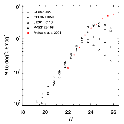
Figure 1: $U$-band number counts from the four fields Q0042-2627 (black crosses), HE0940-1050 (diamonds), J1201+0116 (triangles) and PKS2126-158 (squares). The counts of Metcalfe et al. (2001) from the William Herschel Deep Field are shown for comparison (red crosses).

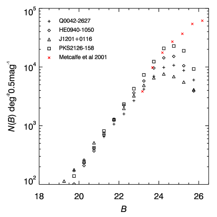
Figure 2: $B$-band number counts from the four fields Q0042-2627 (black crosses), HE0940-1050 (diamonds), J1201+0116 (triangles) and PKS2126-158 (squares). The counts of Metcalfe et al. (2001) from the William Herschel Deep Field are shown for comparison (red crosses).

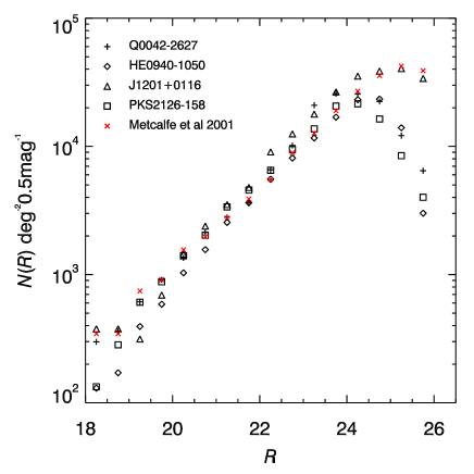
Figure 3: $R$-band number counts from the four fields Q0042-2627 (black crosses), HE0940-1050 (diamonds), J1201+0116 (triangles) and PKS2126-158 (squares). The counts of Metcalfe et al. (2001) from the William Herschel Deep Field are shown for comparison (red crosses).

2.5 Selection Criteria

We perform a photometric selection based on that of Steidel et al. (1996, 2003), but applied to the $U$, $B$ and $R$ band imaging available from our imaging survey. As in Steidel et al. (2003) our selection takes advantage of the Lyman-Break at 912Å and the Ly$\alpha$-forest passing through the $U$-band and into the $B$-band in the redshift range $2.0<z<3.5$. To establish the selection in the Vega $UBR$ system, we convert from the Steidel et al. (2003) selections using the photometric transformations of Steidel & Hamilton (1993), moving from the $U_{n}G{\cal R}$ AB system to the Johnson-Morgan/Kron-Cousins Vega photometry. The approximate transformations (Steidel & Hamilton, 1993) are as follows: $U_{n}=U+0.75$, $G=B-0.17$ and ${\cal R}=R+0.14$ and transform the Steidel et al. (2003) selection to $(B-R)\leq 1.51$ and $(U-B)\geq(B-R)-0.23$.

We also take into account model colour tracks calculated using GALAXEV (Bruzual & Charlot, 2003). The tracks are shown in Figs. 4 and 5 (solid black curves). We use a Salpeter initial mass-function, assuming solar metallicity with a galaxy formed at $z=6.2$ (i.e. with an age of 12.6 Gyr at $z=0$) and a $\tau=9$ Gyr exponential SFR. The three different curves show the effect of dust extinction with a model given by (left to right) $\tau_{\nu}=0.5$, $\tau_{\nu}=1.0$ and $\tau_{\nu}=2.0$, where $\tau_{\nu}=2.0$, where $\tau_{\nu}$ is the effective absorption (Charlot & Fall, 2000). The models agree well with the transformation of the Steidel et al. (2003) selection criteria, although the dustier models do suggest a greater extension of the $z>3$ population to higher values of $(B-R)$ than the Steidel et al. (2003) criteria.

Based on the models and the Steidel et al. (2003) criteria, we develop a number of selection criteria in the $UBR$ system. The key modifications that we make from our initial colour-cut estimates based on the Steidel et al. (2003) cuts are to extend the selection further redwards in $(B-R)$ and to align the $(U-B)-(B-R)$ axis with the stellar locus in the $UBR$ plane, which has a slope of $(U-B)\sim 1.25(B-R)$. We note that the first of these modifications risks increasing the number of contaminants in the form of M-stars (Steidel & Hamilton, 1993) and the second increases the risk of contaminants in the form of lower redshift galaxies. However, given the large number of slits available to us with the VLT VIMOS spectrograph, we deem the risk of increased levels of contamination acceptable, whilst extending the colour-cuts can allow the observation of dusty $z>3$ objects as well as $z\approx 3$ galaxies which may be scattered out of the primary selection area due to photometric errors on these faint objects. As such we use four selection criteria with different priorities for spectroscopic observation (taking advantage of the object priority system in arranging the VIMOS slit masks). These selection criteria are as follows:

• LBG_PRI1

  1. $23<R<25.5$

  2. $U-B>0.5$

  3. $B-R<0.8(U-B)+0.6$

  4. $B-R<2.2$

• LBG_PRI2

  1. $23<R<25.5$

  2. $U-B>0.0$

  3. $B-R<0.8(U-B)+0.8$

  4. $B-R<2.8$

• LBG_PRI3

  1. $23<R<25.5$

  2. $-0.5<U-B<0.0$

  3. $B-R<0.8(U-B)+0.6$

• LBG_DROP

  1. $23<R<25.5$

  2. No U detection

  3. $B-R<2.2$

LBG_PRI1 is our primary sample and selects candidates that are expected to be the most likely $2.5<z<3.0$ galaxies. The LBG_PRI2 sample targets objects with colours closer to the main sequence of low-redshift galaxies than the LBG_PRI1 objects. This sample is therefore expected to include a greater level of contamination from low redshift galaxies. In addition, based on the path of the evolution tracks in Figs. 4 and 5, we also expect the $z>2.5$ population that this selection samples to have, on average, a lower redshift than the LBG_PRI1 sample. The next selection sample, LBG_PRI3, takes this further and is intended to target a $2.0<z<3.0$ galaxy redshift based on the evolution tracks. Finally, we select a sample of $U$-dropout objects (LBG_DROP) with detections in only our $B$ and $R$ band data.

In none of the above samples do we attempt to remove stellar-like objects due to the risk of losing good LBG candidates. The half-light radius of $z\approx 3$ LBGs has been shown to be on average $0.4\arcsec$ and so will not be resolved in our data, which is mostly taken under conditions of $>0.8\arcsec$ seeing.

We apply these selection criteria to four of our QSO fields: Q0042-2627, HE0940-1050, J1201+0116 and PKS2126-158. The candidate selection for the J0124+0044 field was performed separately and is discussed in Bouché & Lowenthal (2004). Figs. 4 and  5 show the four selection criteria applied to these four fields. The selection boundaries are shown by the red, green and blue lines for the LBG_PRI1, LBG_PRI2 and LBG_PRI3 selections respectively. Objects selected as candidates by each criteria set are shown by red, green, blue and cyan points for the LBG_PRI1, LBG_PRI2, LBG_PRI3 and LBG_DROP selections respectively. The grey contours in each plot show the extent of the complete galaxy population in each of the fields.

Returning to the depths of our fields, we now compare these to those of previous studies in the selection of LBGs. We note that Steidel et al. (2003) used photometry with mean 1$\sigma$ depths of $\left<\sigma(U_{n})\right>=28.3$, $\left<\sigma(G)\right>=28.6$ and $\left<\sigma({\cal R})\right>=28.0$, whilst their imposed ${\cal R}$ band limit was ${\cal R}=25.5$. Using the transformations of Steidel & Hamilton (1993), the Steidel et al. (2003) 1$\sigma$ limits correspond to $U=27.55$, $B=28.77$ and $R=27.86$ in the Vega system. Comparing this to the average depths in our own fields, we have mean $3\sigma$ depths of $U=26.2$, $B=26.8$ and $R=26.3$, which equate to $1\sigma$ depths of $U=27.4$, $B=28.0$ and $R=27.5$, largely comparable to the Steidel et al. (2003) imaging data.

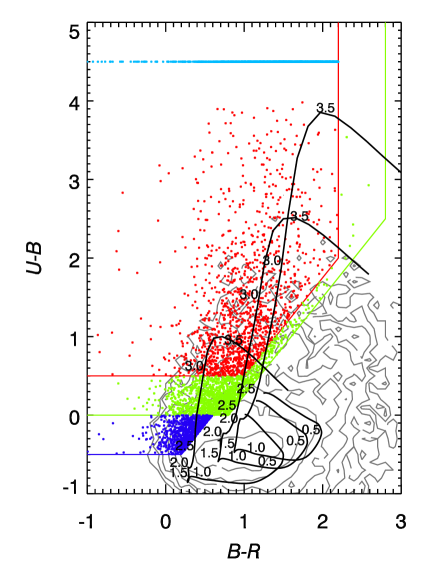
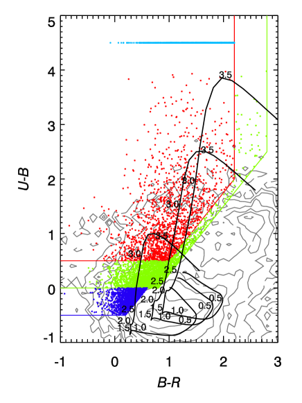
Figure 4: Our selection criteria in $UBR$ colour space shown for the Q0042-2627 (left) and HE0940-1050 (right). The red line and points show the LBG_PRI1 selection, the green line and points show the LBG_PRI1 selection, the blue line and points show the LBG_PRI3 selection and the cyan line at $U-B=4.5$ shows the LBG_DROP selection. The grey contours show the entire galaxy population in the fields. The black lines show the galaxy evolution model for a galaxy with a $\tau=9$Gyr exponential SFR formed at $z=6.2$ and are labelled with values of observed redshift from $z=3.83$ to $z=0$.

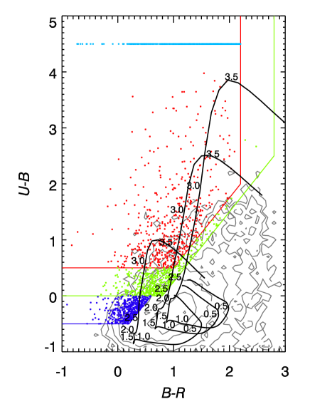
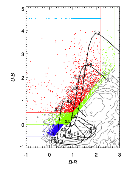
Figure 5: As in Fig. 4 but for the J1201+0116 and PKS2126-158 fields (left to right).

The numbers of objects selected by each selection for each field are given in Table 2. These candidate selections were used as the basis for the spectroscopic work which is described in the following sections.

Table 2: Number of candidate high redshift objects in each of the selected fields. Note that candidates in the J0124+0044 were selected as described in Bouché & Lowenthal (2004) and not using the four selection criteria sets described in this paper.

Field	LBG_PRI1	LBG_PRI2	LBG_PRI3	LBG_DROP	Total
Q0042-2627	1,366	1,381	650	1,390	4,787
J0124+0044					3,679
HE0940-1050	1,646	2,249	741	1,042	5,678
J1201+0116	477	487	469	606	2,029
PKS2126-158	1,380	2,119	713	667	4,879
Total	4,869	6,236	2,573	3,705	21,062
Observed spectroscopically	730	569	256	999	2,554

2.6 QSO Candidate Selection

At redshifts of $z\approx 3$, the observed optical spectra of QSOs and galaxies exhibit similar shapes, both being heavily influenced by the Lyman break feature. We therefore add to our targets a number of QSO candidates in each field (except J0124+0044) using the following selection, which is closely based on our high-priority $z\approx 3$ LBG selection:

1. CLASS_STAR $>0.8$

2. $U-B>0.5$

3. $B-R<0.8(U-B)+0.8$

4. $0.0<B-R<2.2$

The magnitude limits used with this selection were $20<R<23$ in the Q0042-2627 and J1201+0116 fields and $18<R<22$ in the HE0940-1050 and PKS2126-158 fields for which we had obtained shallow imaging and could therefore select brighter objects more reliably.

As with the LBGs, QSOs at $z>2$ may be selected by the passage of the Lyman-break through the $U$-band (e.g. Richards et al. 2009). This selection is therefore based on the LBG selection, but constrained to brighter magnitudes and stellar-like objects only. This selection gives 71, 39, 15 and 38 QSO candidates in the Q0042-2627, HE0940-1050, J1201+0116 and PKS2126-158 fields respectively. Note that only a small number of these have actually been observed spectroscopically as the LBG candidates remained the higher priority.

3 Spectroscopy

3.1 Observations

We observed our LBG candidates using the VIMOS instrument on the VLT UT3 (Melipal) between September 2005 and March 2007. As described earlier, the VIMOS camera consists of four CCDs, each with a field of view of $7\arcmin\times 8\arcmin$, arranged in a square configuration, with $2\arcmin$ gaps between the field-of-views of adjacent chips. Each observation therefore covers a field of view of $16\arcmin\times 18\arcmin$ with $224~{}{\rm arcmin}^{2}$ being covered by the CCDs. The instrument was set up with the low-resolution blue grating (LR_Blue) in conjunction with the OS_Blue filter, giving a wavelength coverage of 3700Å to 6700Å and a resolution of 180 with $1\arcsec$ slits, corresponding to 28Å FWHM at 5000Å. The dispersion with this setting is 5.3Å per pixel. We note that this configuration also projects the zeroth diffraction order onto the CCDs.

Given the size of our imaging fields ($36\arcmin\times 36\arcmin$) it was possible to target 4 distinct sub-fields with the VIMOS field of view. We have therefore observed a total of 19 sub-fields across our 5 fields, i.e. 4 sub-fields in each field except for HE0940-1050 in which only 3 sub-fields were achievable due to the CCD malfunction during the imaging observations. Each sub-field was observed with $10\times 1,000$s exposures, apart from sub-field three of the PKS2126-158, which was observed with only $4\times 1,000$s due to time constraints in the VIMOS schedule. All observations were performed during dark time, with $<0.8\arcsec$ seeing and $<1.3$ air mass.

Slit masks for each quadrant of each sub-field were designed using the standard VIMOS mask software, VMMPS. We used minimum slit lengths of $8\arcsec$, which equates to 40 pixels given the pixel scale of $0.205\arcsec/\textrm{pixel}$. With the effectively point-like nature of our sources and our maximum seeing constraint of $0.8\arcsec$ this allows us a minimum of $\approx 7\arcsec$ for sky spectra per slit (with which to perform the sky-subtraction when extracting the spectra). Using the VMMPS software with the LR_Blue grism we were able to target up to $\approx 60-70$ objects per quadrant (i.e. $\approx 250$ objects per sub-field), depending on the sky density of the candidate objects. For the spectroscopic observations, we predominantly used the selections as given in section 2.5, however to optimize the spectroscopic observations some flexibility was employed in including small numbers of objects outside the selection criteria. However, we note that the LBG_PRI3 selection was not employed in the spectroscopic observations in the first observations (i.e. the observations of HE0940-1050 and PKS2126-158), whilst the magnitude limit used for selecting objects to observe for later fields was reduced from $R=25.5$ to $R=25$. The total number of spectroscopically observed objects was 3,562.

Table 3: Details of the spectroscopic data acquired in each of our five target fields. Coordinates are given for the targeting centre of each sub-field.

Field	Sub-field	$\alpha$	$\delta$	Dates	Exp time	Seeing
		(J2000)	(J2000)		(s)
Q0042-2627	f1	00:45:11.14	-26:04:22.0	8-10,15/08/2007	$10,000$	$0.6-1.0\arcsec$
Q0042-2627	f2	00:43:57.30	-26:04:22.0	18-19/08/2007 & 5-6/09/2007	$10,000$	$0.9-1.0\arcsec$
Q0042-2627	f3	00:45:10.35	-26:19:06.9	11-12/09/2007	$10,000$	$0.9-1.0\arcsec$
Q0042-2627	f4	00:43:55.97	-26:19:16.1	7,10/09/2007	$10,000$	$0.9-1.0\arcsec$
J0124+0044	f1	01:24:41.82	+00:52:18.8	1-2,4/11/2005	$10,000$	$0.8-0.9\arcsec$
J0124+0044	f2	01:23:32.06	+00:52:13.1	5,29,31/10/2005	$10,000$	$0.6-1.0\arcsec$
J0124+0044	f3	01:23:31.29	+00:37:02.0	19-20/09/2007	$10,000$	$0.8-1.0\arcsec$
J0124+0044	f4	01:24:41.86	+00:36:51.4	4/12/2005 & 22/08/2006	$10,000$	$0.8-0.9\arcsec$
HE0940-1050	f1	09:42:08.02	-11:08:14.2	26-27,29/01/2006	$10,000$	$0.5-0.8\arcsec$
HE0940-1050	f2	09:43:21.53	-11:08:35.0	30-31/01/2006, 1,25/02/2006 & 1/03/2006	$10,000$	$0.5-1.0\arcsec$
HE0940-1050	f3	09:43:21.58	-10:54:31.8	14,19/12/2007 & 31/01/2008	$10,000$	$0.6-1.0\arcsec$
J1201+0116	f1	12:02:14.01	+01:09:09.9	13-15/04/2007 & 17/04/2007	$10,000$	$0.6-1.0\arcsec$
J1201+0116	f2	12:01:10.01	+01:09:09.9	23/04/2007 & 8,11,14/05/2007	$10,000$	$0.4-0.9\arcsec$
J1201+0116	f3	12:01:10.04	+01:24:09.8	16-17/05/2007	$10,000$	$0.5-0.9\arcsec$
J1201+0116	f4	12:02:14.07	+01:24:08.0	18/05/2007 & 6,8,10/02/2008	$10,000$	$0.6-0.7\arcsec$
PKS2126-158	f1	21:29:59.57	-15:31:30.2	17/08/2006 & 1,21-26/09/2006	$10,000$	$0.7-1.0\arcsec$
PKS2126-158	f2	21:28:46.20	-15:31:29.9	5-6/08/2005	$10,000$	$0.6-1.0\arcsec$
PKS2126-158	f3	21:30:00.41	-15:47:18.3	27/09/2006	$4,000$	$0.8-1.0\arcsec$
PKS2126-158	f4	21:28:46.27	-15:47:11.9	9-11,25,29/08/2005	$10,000$	$0.7-0.9\arcsec$

3.2 Data reduction

Bias frames were obtained by the VLT service observers at the beginning of each night of observations. Lamp-flats were also taken with each of the masks with the observation setup in place (i.e. the OS_Blue filter and LR_Blue grism). These were also taken by the service observers at the beginning of each night’s observation. Arc frames were taken during the night with each of the masks with the LR_Blue grism and OS_Blue filter.

Data reduction was performed using the VIMOS pipeline software, ESOREX. Firstly the bias frames were combined to form a master bias using VMBIAS. The flat frames were then processed and combined using the VMSPFLAT recipe. VMSPCALDISP was then used to process (bias subtract and flat-field) the arc lamp exposure and to determine the spectral distortions of the instrument. We measured a mean RMS on the inverse dispersion solution (IDS) of $2.3\pm 0.6$ Å. With the bias, flat and arc exposures all processed, the object frames were reduced and combined using the VMMOSOBSSTARE recipe to produce the reduced 2-D spectra. The spectra have not been fully flux calibrated, however we have applied the master response curves for the LR_Blue grism to correct for the effects of the grism as a function of wavelength.

We extract the 1-D spectra using purpose-written IDL routines. For each spectrum, we first fit the shape of the spectrum across the slit. This is implemented by binning the 2-D aperture along the dispersion axis and then fitting a Gaussian profile to each bin to find the centre of the object signal in each bin. We then fit the resultant spread in the central pixel with a 4th order polynomial function. We then lay an object aperture with a width of $n_{ap}$ pixels over the object and a sky aperture covering all of the usable sky region in the slit. The object and sky spectra are then taken as being the mean over the widths of their respective apertures. Finally, we subtract the sky spectrum from the object spectrum to produce the final object spectrum. The dominant remaining sky-contamination after sky-subtraction were the strong sky emission lines [OI]5577 Å  [NaI]5890 Å and [OI]6300 Å.

Figure 6: Mean signal-to-noise per resolution element (28Å) in the wavelength range 4100Å$<\lambda<$5300Å as a function of $R$-band magnitude in our VLT VIMOS spectra with integration times of 10,000s.

We estimate the signal-to-noise by taking the RMS of the sky aperture in each wavelength bin and dividing by $\sqrt{n_{ap}}$, where $n_{ap}$ is the width of the aperture used to extract the 1-D spectrum of a given object. Fig. 6 shows the mean signal-to-noise per resolution element (i.e. 28Å) in the wavelength range 4100Å$<\lambda<$5300Å in our sky-subtracted spectra as a function of source $R$-band magnitude. The selected range covers many of the key emission and absorption lines exhibited in LBGs in the redshift range $2.5<z<3.5$, whilst excluding the strong sky lines. The points in Fig. 6 show the mean spectrum SNR per resolution element, whilst the error bars show the standard deviation within each bin. In the faintest bin ($25.25<R<25.5$), we achieve a mean continuum signal-to-noise of $\approx 3.5$. This rises to a continuum signal-to-noise $\approx 9$ for our brightest objects ($23<R<23.25$).

3.3 Object Identification

We perform the object identification for each slit individually by eye. Given the wavelength range covered by the LR_Blue grism combined with the redshift range of our targets, $2<z<3.5$, there are several key spectral features that facilitate the identification of those targets. These are primarily:

• Lyman limit, 912Å;

• Ly$\beta$ emission/absorption, 1026Å

• OVI 1032Å, 1038Å;

• Ly$\alpha$ forest, $<$1215.67Å;

• Ly$\alpha$ emission/absorption, 1215.67Å;

• Inter-stellar medium (ISM) absorption lines:

  • SiII 1260.4Å;

  • OI$+$SiII 1303Å;

  • CII 1334Å;

  • SiIV doublet 1393Å & 1403Å;

  • SiII 1527Å;

  • FeII 1608Å;

  • AlII 1670Å;

• CIV doublet absorption/emission, 1548-1550Å.

The most prominent of these features is most frequently the Ly$\alpha$ emission/absorption feature at 1215Å. However, as discussed by Shapley et al. (2003), the observed optical (rest-frame UV) absorption and emission features are thought to originate from an outflowing shell of material surrounding the core nebular region of the galaxy. These features do not therefore represent the redshift of the rest-frame of the galaxy but in fact of these outflows.

For each confirmed LBG we measure independently the redshift of the Ly$\alpha$ emission/absorption feature and the redshift of the ISM absorption features. In order to measure the Ly$\alpha$ redshift, we fit the feature with a Gaussian function allowing the amplitude, central wavelength and width to be free parameters. From these we determine the redshift and line-width of the feature. We note that absorption blue-wards of the emission wavelength produces an asymmetry in the observed emission line, however given the modest resolution of our observations the Gaussian fit is preferred to any more complex asymmetric fitting to the emission line.

We have performed an estimate of the accuracy of our redshift results by repeating the spectral line fitting method with mock spectra. Each mock spectrum consists of a single Gaussian emission line (i.e. $f=Ae^{-(\lambda-\lambda_{\circ})^{2}/2\sigma^{2}}$) at a random redshift in the range $2.5<z<3.5$ and a FWHM of $1680~{}{\rm kms}^{-1}$ corresponding to a Gaussian width of $\sigma=850~{}{\rm kms}^{-1}$ (equivalent to the resolution of the instrument). Gaussian random noise was then added to the basic emission line shape to give the required signal-to-noise. For each mock spectrum, we then performed the Gaussian fitting, iteratively performing the process for a total of $10^{4}$ mock spectra at a given signal-to-noise. The difference between the input redshift and the Gaussian line fitting redshift was then measured for each of the iterations and the error estimated from the distribution of this difference in input and measurement. The process was repeated, increasing the emission line peak flux from 1 to 20$\times$ the Gaussian noise width.

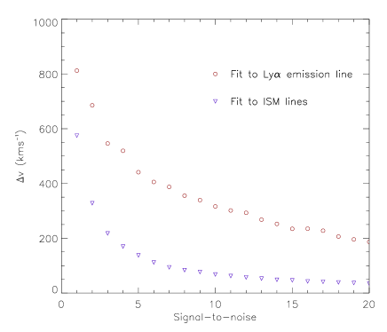
Figure 7: Estimate of the accuracy of the Gaussian line-fitting based on iteratively fitting mock spectra with Gaussian random noise. The open circles show the results of applying the fitting method to a single emission line spectrum with a range of signal-to-noise (where the signal-to-noise is defined as the ratio between the peak signal and the width of the Gaussian noise). The blue triangles show the result of the same method applied to a simple absorption line spectrum including the ISM lines: SiII (1260Å), OI+SiII (1303Å), CII (1336Å) and SiIV (1393Å, 1402Å).

The results are given in Fig. 7, where the measured accuracy is plotted as a function of the calculated signal-to-noise (red circles). Further to this, we measure the distribution of Ly$\alpha$ emission peak signal-to-noise in our galaxy sample, which is shown in Fig. 8 as a percentage of the total number of LBGs exhibiting Ly$\alpha$ emission. If we now compare these two plots, we see that $\approx 90\%$ of our emission line LBGs have an emission line signal-to-noise of $>3$, which suggests that $90\%$ of the Ly$\alpha$ emission line redshifts have velocity errors of less than $\approx 550~{}{\rm kms}^{-1}$. Further, the median Ly$\alpha$ emission line signal-to-noise is $\approx 5.5$ which gives a velocity error of $\approx 400~{}{\rm kms}^{-1}$. Our higher quality spectra (i.e. the top $20\%$) however, are estimated to achieve velocity errors on the Ly$\alpha$ emission line redshifts as small as $\approx 200~{}{\rm kms}^{-1}$.

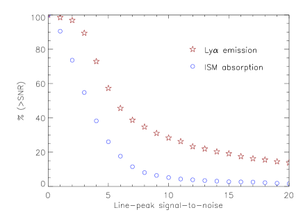
Figure 8: The distribution of Ly$\alpha$ emission line (red stars) and ISM absorption line (blue circles) signal-to-noise measurements in our LBG sample. The calculated signal-to-noise is the ratio between the emission/absorption line peak (after subtracting the continuum) and the measured noise. The final ISM signal-to-noise value is taken as the median of the calculated values for the ISM lines used. See Fig. 7 for the estimated velocity errors based on the feature signal-to-noise.

Where feasible, we also attempt to measure the redshift of the ISM absorption lines based on the SiII, OI+SiII, CII and SiIV doublet (despite being a mixture of high and low ionization lines we note that they are all measured to have comparable velocity offsets in Shapley et al. 2003, at least within the resolution constraints afforded by our observations). We primarily use absorption lines between $1215\mbox{\AA}\lesssim\lambda_{rest}\lesssim 1500\mbox{\AA}$ as these remain within the wavelength coverage of the low-resolution blue grism over the full redshift range (i.e. $2\lesssim z\lesssim 3.5$) of our survey. Measuring the individual absorption lines in most of our spectra is difficult given the SNR of the absorption features in our spectra, however our ability to estimate the redshift of the ISM lines can be greatly improved by attempting to determine the mean ISM redshift by fitting the five lines simultaneously.

To evaluate this method we repeat the iterative error analysis performed for the Ly$\alpha$ emission line fitting, but fitting five absorption lines (with $\sigma_{ISM}=850~{}{\rm kms}^{-1}$) simultaneously. Again we measure the offset between the input redshift and the output redshift measured from the Gaussian line fitting. The result is again plotted in Fig. 7 (blue triangles), whilst the distribution of ISM signal-to-noise measurements in the data is again given in Fig. 8. This suggests that we may reasonably expect a significant improvement in the estimated redshift compared to measuring just a single line. We now predict an accuracy of $\approx 200~{}{\rm kms}^{-1}$ at a signal-to-noise of $\approx 3$, which based on Fig. 8 accounts for $55\%$ of our sample.

With the Ly$\alpha$ and ISM redshifts determined, we estimated the intrinsic redshifts, $z_{\mathrm{int}}$, of our LBG sample using the relations of Adelberger et al. (2005a). These relations were derived from a sample of 138 LBGs observed spectroscopically in both the optical and the near infrared and are based on the offsets found between the Ly$\alpha$ plus ISM lines and the nebular emission lines, [OII]3727Å, H$\beta$, [OIII]5007Å and H$\alpha$. These lines are all associated with the central star-forming regions of LBGs as opposed to the outflowing material and are thus expected to be more representative of the intrinsic redshift of a given LBG. The relations of Adelberger et al. (2005a) that we use here are as follows:

For LBGs with only a redshift from the Ly$\alpha$ emission line we used:

$$z_{\mathrm{int}}=z_{\mathrm{Ly}\alpha}-0.0033-0.0050(z_{\mathrm{Ly}\alpha}-2.7)$$ (1)

For objects with Ly$\alpha$ absorption and a measurement of $z_{\mathrm{ISM}}$ we used:

$$z_{\mathrm{int}}=z_{\mathrm{ISM}}+0.0022+0.0015(z_{\mathrm{ISM}}-2.7)$$ (2)

And for objects with redshifts measured from both the Ly$\alpha$ emission line and the ISM absorption lines we used:

$$z_{\mathrm{int}}=\overset{\_}{z}+0.070\Delta z-0.0017-0.0010(\overset{\_}{z}-2.7)$$ (3)

where $\overset{\_}{z}$ is the mean of the Ly$\alpha$ redshift ($z_{\mathrm{Ly}\alpha}$) and the ISM absorption line redshift ($z_{\mathrm{ISM}}$) and $\Delta z\equiv z_{\mathrm{Ly}\alpha}-z_{\mathrm{ISM}}$. Adelberger et al. (2005a) quote rms scatters of $\sigma_{z}=0.0027$ ($200~{}{\rm kms}^{-1}$), $0.0033$ ($250~{}{\rm kms}^{-1}$) and $0.0024$ ($180~{}{\rm kms}^{-1}$) respectively for each of the above relations based on their application to their optical and IR spectroscopic sample of LBGs.

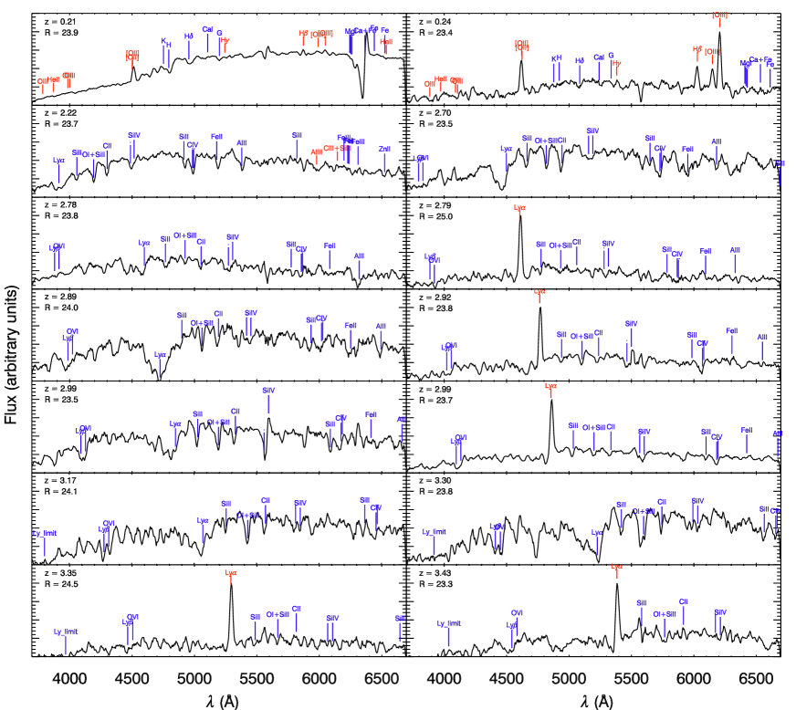
Figure 9: Example spectra taken using 10,000s integration time with the LR_Blue grism on the VLT VIMOS instrument. The top two spectra are examples of contaminating low-redshift galaxies. The remaining 12 panels show LBG spectra exhibiting both Ly$\alpha$ emission and absorption over the redshift range $2<z<3.5$. ISM lines are also clearly identifiable in the individual LBG spectra as is the Lyman limit. Both galaxy redshift and apparent $R$-band magnitude (Vega) are quoted for each object. Note that all the above spectra have been binned to $\approx 16$Å.

As well as $z\approx 3$ galaxies, our selection also samples a number of contaminating objects. These consist of low-redshift emission line galaxies (identified by [OII]3727Å, H$\beta$, [OIII]5007Å and H$\alpha$ emission), low-redshift Luminous Red Galaxies (LRGs - identified by [OII]3727Å emission, Ca H, K absorption and the 4000Å break) and faint red stars (mostly M and K-type stars). We show examples of the spectra of several LBGs and contaminant low-redshift galaxies taken with the VLT VIMOS in this survey in Fig. 9 (note that these are not flux-calibrated spectra).

All identified objects, including stars and low-redshift galaxies, were assigned a quality rating, q, based on the confidence of the identification. The value of q was assigned on a scale of 0 to 1, with 1 being the most confident and 0 being unidentified. All objects with $q<0.5$ were rejected as spurious identifications and are not included in the spectroscopic catalogue used in the remainder of this work. LBGs were generally classified as follows:

• 0.5 - Ly$\alpha$ emission or absorption line evident plus some ’noisy’ ISM absorption features.

• 0.6 - Ly$\alpha$ emission or absorption plus some ISM absorption features.

• 0.7 - Ly$\alpha$ emission or absorption plus most ISM absorption features.

• 0.8 - Clear Ly$\alpha$ emission or absorption plus all ISM absorption features.

• 0.9 - Clear Ly$\alpha$ emission or absorption plus high signal-to-noise ISM features.

With this classification scheme, we have identified 392, 254, 170, 111 and 93 $z>2$ galaxies with $q=$0.5, 0.6, 0.7, 0.8 and 0.9 respectively.

3.4 Sky Density, Completeness & Distribution

We summarize the numbers of objects observed in Table 4. Our mean sky density for successfully identified LBGs is $0.24\text{arcmin}^{-2}$, whilst the percentage of $z>2$ galaxies in the entire observed sample (the success rate given in table 4) is 27.5%. The remaining observed objects are a mix of low-redshift galaxies, stars and unidentified objects (generally very low-signal to noise spectra). In the worst case field (J1201+0116), we have a greater number of low-redshift galaxies than high redshift detections. We attribute this to the relatively poor depth of the imaging observations in this field. We also note that the PKS2126-158 field is at a relatively low galactic latitude and thus was a higher proportion of contamination by galactic stars. However, the field still shows a high proportion of $z>2$ galaxies.

Table 4: Summary of objects identified in the VLT VIMOS observations. The success rate is the number of successfully identified LBGs divided the total number objects observed. Example spectra of the high-redshift and low-redshift galaxies are shown in Fig. 9. All 10 identified $z>2$ QSO spectra are provided in Fig. 16.

Field	Subfields	Slits	Galaxies	QSOs	Galaxies	Stars	Success rate
			$z>2$	$z>2.0$	$z<2.0$
Q0042-2627	4	876	264 ($0.29\text{arcmin}^{-2}$)	1	106	5	30.1%
J0124+0044	4	832	264 ($0.29\text{arcmin}^{-2}$)	0	54	18	31.7%
HE0940-1050	3	501	169 ($0.25\text{arcmin}^{-2}$)	1	48	36	33.7%
J1201+0116	4	699	120 ($0.13\text{arcmin}^{-2}$)	5	144	72	17.2%
PKS2126-158	4	654	203 ($0.23\text{arcmin}^{-2}$)	3	49	126	31.0%
Total	19	3562	1020 ($0.24\text{arcmin}^{-2}$)	10	401	257	28.6%

In Fig. 10 and Table 5 we summarize the redshift distributions of each of our sample selections in our observed fields. The overall redshift distribution across all fields is shown in the bottom panel of Fig. 10, with the black histogram showing the redshift distribution from $UBVI$ selected objects from J0124+0044 and the red, green, blue and cyan histograms showing the LBG_PRI1, LBG_PRI2, LBG_PRI3 and LBG_DROP selections respectively. The overall mean redshift for our confirmed LBG sample is $\overset{\_}{z}=2.85\pm 0.34$. It is evident from the redshift distributions that the separate selection sets give slightly differing (but overlapping) segments in redshift space. As may be expected, the LBG_DROP selection is the most biased towards the higher end of our redshift distribution, with an overall mean redshift across all our samples of $\overset{\_}{z}=2.99$. The LBG_PRI1 selection provides a redshift range of $2.90\pm 0.32$, whilst the LBG_PRI2 and LBG_PRI3 give comparable redshift distributions of $2.67\pm 0.26$ and $2.67\pm 0.31$ respectively. We also show the redshift distributions for each individual field in the top five panels of Fig. 10, with the LBG_PRI1, LBG_PRI2, LBG_PRI3 and LBG_DROP identically to that in the ’all fields’ plot. In each field we again see that the LBG_PRI3 and LBG_PRI2 selections preferentially select the lowest redshift ranges followed by LBG_PRI1 and LBG_DROP showing the highest redshift range (although this is less pronounced in the J1201+0116 field in which the imaging depths were least faint).

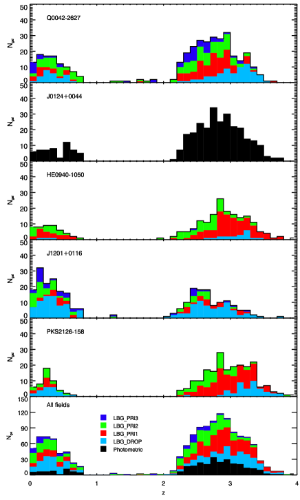
Figure 10: Differential redshift distribution in each of our fields and summed over all fields. We show the number counts split by selection criteria: LBG_DROP (cyan histograms), LBG_PRI1 (red histograms), LBG_PRI2 (green histograms) and LBG_PRI3 (blue histograms). The mean redshifts for each selection are given in table 5.

Table 5: Redshift ranges of $z>2$ galaxies identified from each of our photometric selections.

Field	LBG_PRI1	LBG_PRI2	LBG_PRI3	LBG_DROP
Q0042-2627	$2.74\pm 0.28$	$2.66\pm 0.26$	$2.67\pm 0.30$	$3.04\pm 0.28$
J0124+0044	$2.86\pm 0.34$
HE0940-1050	$3.02\pm 0.33$	$2.67\pm 0.29$	$2.85\pm 0.39$	$3.10\pm 0.21$
J1201+0116	$2.71\pm 0.29$	$2.45\pm 0.41$	$2.61\pm 0.29$	$2.74\pm 0.33$
PKS2126-158	$2.98\pm 0.29$	$2.72\pm 0.27$	n/a	$3.30\pm 0.29$
All fields	$2.90\pm 0.32$	$2.66\pm 0.28$	$2.67\pm 0.30$	$2.99\pm 0.36$

We illustrate the distribution of our spectroscopic LBG sample in each of our 5 fields in Fig. 11. The fields are ordered by R.A. top to bottom and all identified $z>2$ galaxies (filled blue circles) are shown along with all known $z>2$ QSOs identified from the NASA Extragalactic Database. We also plot the positions of QSOs identified in our VIMOS observations and AAOmega QSO survey, which is described further in Crighton et al. (2010).

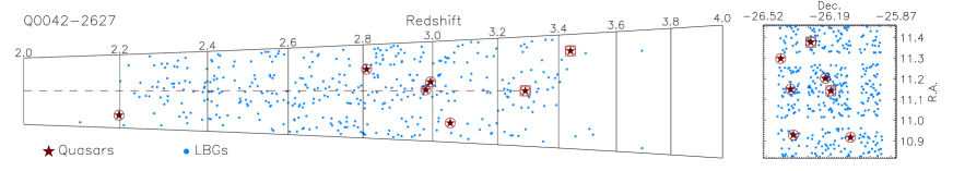
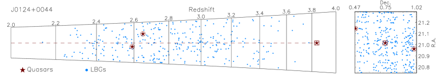
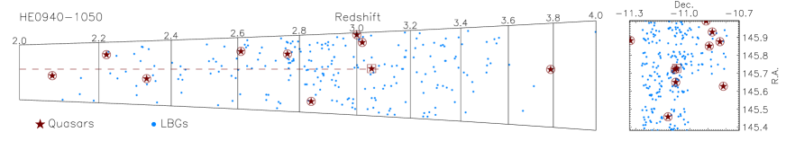
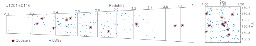
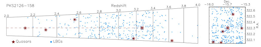
Figure 11: Distribution in R.A., Declination and redshift for each of our five fields. Spectroscopically confirmed LBGs are marked by blue filled circles and known QSOs by dark red stars. We also identify those QSOs with low-resolution spectra available (red circles, i.e. VLT VIMOS and AAT AAOmega), medium-resolution spectra (red crosses, i.e. SDSS - SDSS J1201+0116 only) and high-resolution spectra (red squares, i.e. VLT UVES, Keck HIRES).

In Fig. 12 we plot the number of identified LBGs in magnitude bins for each of our fields. The filled histograms show the cumulative numbers of successfully identified objects (including interlopers as well as $z>2$ galaxies) split by their selection criteria. LBG_DROP selected objects are shown by the cyan histogram, LBG_PRI1 by the red histogram, LBG_PRI2 by the green histogram and LBG_PRI3 by the blue histogram. The distribution of all spectroscopically observed objects is given by the solid line histogram in each case. As the J0124+0044 objects were not selected using the same selection criteria, these are simply left as a single group shown by the filled black histogram. In all fields, we see that we are successfully identifying objects down to the magnitude limit of R$=25.5$ (I$=25$ in the case of J0124+0044), although a significant number of objects remain unidentified in each field at the fainter magnitudes as spectral features become more difficult to discern in the spectra. We note also that the shapes of the overall magnitude distributions are biased more towards brighter objects in the Q0042-2627 and J1201+0116 fields in which a greater number of LBG_PRI3 objects are included (and also the imaging depths achieved in these fields are shallower than in the other fields).

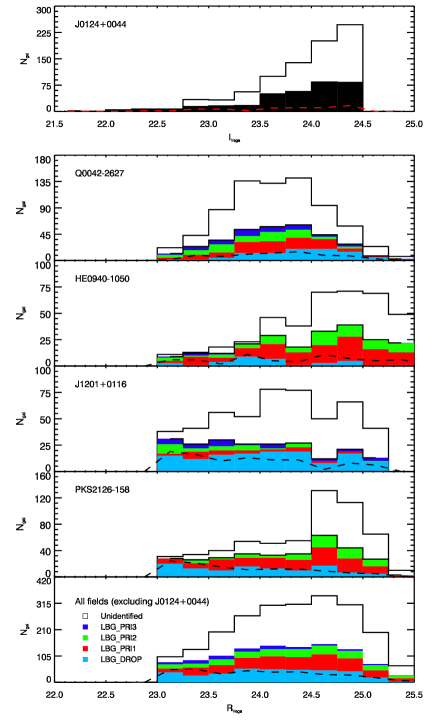
Figure 12: Number counts as a function of R_Vega magnitude for all fields, except for J0124+0044 in which I_Vega is used. The shaded histograms show the numbers of successfully identified objects with the colour coding the same as in Fig. 10: the cyan histogram shows counts of LBG_DROP objects, the red shows LBG_PRI1 objects, the green shows LBG_PRI2 objects and the blue shows LBG_PRI1 objects. The unshaded histogram shows the total number of candidates observed with VLT-VIMOS in each field (i.e. the gap between the shaded regions and solid line shows the number of unidentified objects as a function of magnitude). Contamination levels from stars and low-redshift galaxies for each field are given by the dashed line in each panel.

In Fig. 13, we show the number counts of our photometrically selected LBGs (open red circles) and the estimated number counts of LBGs (filled red circles) derived from the candidate number counts and the success rate as a function of magnitude (i.e. the number of confirmed LBGs divided by the number of observed candidates). At faint magnitudes we correct the counts for incompleteness in the spectroscopic observations, however we have not made any correction for incompleteness in the original photometry. The number counts of Steidel et al. (2003) are also plotted, showing their candidate number counts (open blue triangles) and number counts corrected for contamination (filled blue triangles). The two data-sets show good agreement over the magnitude ranges sampled.

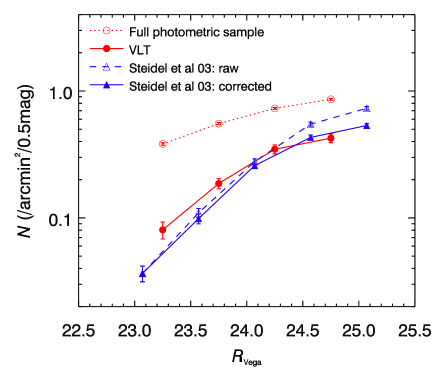
Figure 13: Sky densities of the LBG sample as a function of $R_{\mathrm{Vega}}$ magnitude. The red open circles give the total densities of objects in our LBG_PRI1, LBG_PRI2 and LBG_DROP photometric selections. The ‘VLT’ densities (filled red circles) are estimated using the total photometric densities multiplied by the fraction of successfully identified LBGs from the VLT spectroscopic observations and are corrected for incompleteness in the spectroscopic sample at faint magnitudes. Raw (open blue triangles) and corrected (filled blue triangles) number counts are also shown from Steidel et al. (2003). Note that we transform the Steidel et al. (2003) AB system ${\cal R}$ magnitudes by $-0.14$ to convert to $R_{\mathrm{Vega}}$ (Steidel & Hamilton, 1993).

3.5 Velocity Offsets and Composite spectra

The galaxy spectra contain a wealth of information as illustrated by the work of Shapley et al. (2003). We now look at how our spectra compare to previous work in terms of the velocity offsets between the different spectral features. For the galaxies that exhibit both measurable Ly$\alpha$ emission and ISM absorption lines, we calculate the velocity offsets between these lines, $\Delta v=v_{em}-v_{abs}$. The distribution of $\Delta v$ for our galaxy sample is shown in Fig. 14. The distribution of velocity offsets exhibits a strong peak with a mean of $\left<\Delta v\right>=625$ with a dispersion of $510~{}{\rm kms}^{-1}$. This compares to a value measured by Shapley et al. (2003) of $650~{}{\rm kms}^{-1}$.

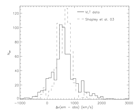
Figure 14: Distribution of the velocity offsets between ISM absorption lines and the Ly$\alpha$ emission line in individual galaxies from our redshift survey (solid histogram). We measure a mean velocity offset between Ly$\alpha$ emission and the ISM lines of $\overset{\_}{\Delta V}=625\pm 510~{}{\rm kms}^{-1}$. The result of Shapley et al. (2003), which has a mean of $650~{}{\rm kms}^{-1}$ is shown by the dashed histogram.

We have produced composite spectra in several Ly$\alpha$ equivalent width bins in order to produce spectra with increased signal-to-noise compared to the individual galaxy spectra. The Ly$\alpha$ profile can be very complex, consisting of both emission and absorption features and this combination often leads to asymmetric profiles with a significant amount of absorption blue-wards of the emission line (Shapley et al., 2003; Kornei et al., 2010). For the purposes of producing composite spectra of the LBGs, we take a relatively simple approach to the measurement of the equivalent widths of our galaxy sample. For a given spectrum, we measure an equivalent width for the emission line if clearly identifiable and if not we make a measurement of the absorption profile. To do this, we fit a polynomial to the continuum and a Gaussian fit to the Ly$\alpha$ line profile and estimate the equivalent width from these fits.

The individual LBG spectra were normalized prior to constructing the composite, using the median of the rest-frame UV continuum in the range $1300\mbox{\AA}\lesssim\lambda_{rest}\lesssim 1500\mbox{\AA}$. After this normalization, we rescale the LBG spectra to the rest-frame and re-binned the spectra before combining the samples to produce the final composite spectra. We note that all the spectra were calibrated using the VIMOS master response curves prior to this process.

The composite spectra are shown in Fig. 15 and are split into (from bottom to top) equivalent width ranges of W$<-20$Å (50 galaxies), -20Å$<$W$<$0Å (134 galaxies), 0Å$<$W$<$5Å (166 galaxies), 5Å$<$W$<$10Å (218 galaxies), 10Å$<$W$<$20Å (181 galaxies), 20Å$<$W$<$50Å (112 galaxies) and W$>$50Å (60 galaxies). Between them, the composites incorporate a total of 921 of the galaxy sample, excluding any objects with $q<0.5$ or with significant contamination, for example from zeroth order overlap. The key emission and absorption features are marked and we can immediately identify both absorption and weak emission for the ISM lines: SiII, OI+SiII, CII, SiIV and CIV. All the features have been marked at $z=0$. The offset between the line centres of the Ly$\alpha$ emission and the ISM absorption lines is evident in these composite spectra, a result of the asymmetry of the Ly$\alpha$, potentially combined with an intrinsic difference between the velocities of the sources of the Ly$\alpha$ emission and the ISM absorption features.

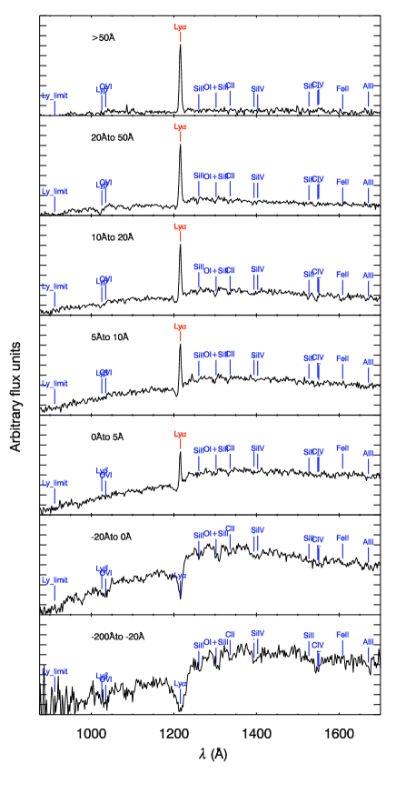
Figure 15: Composite spectra collated from our VLT VIMOS sample. Each spectrum shows the composite of a sub-sample of the LBGs, grouped by Ly$\alpha$ equivalent width measurements. The key UV spectral features discussed in the text (i.e. Ly$\alpha$ and Ly$\beta$ emission/absorption, ISM absorption lines) are all evident in these composite spectra.

3.6 VLT AGN and QSO observations

As discussed earlier, we also targeted a small number of $z\approx 3$ QSO candidates selected from our $UBR$ photometry. In combination with this, due to the similarity in the shape of the spectra of LBGs and QSOs, the LBG selections also produced a handful of faint QSOs and AGN. We present the spectra of these in Fig. 16, whilst the numbers of QSOs in each field are given in table 4. The positions of the observed QSOs are also shown in Fig. 11.

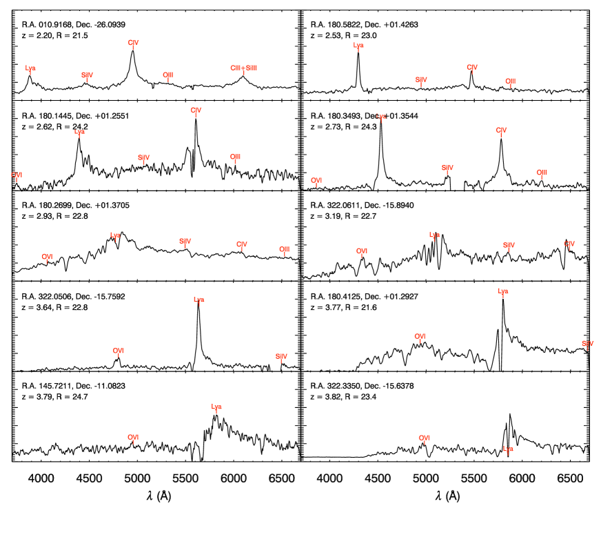
Figure 16: Spectra of the $z>2$ QSOs observed as part of the VLT VIMOS LBG survey. Redshifts and $R$-band magnitudes are given for each QSO and significant broad emission features are marked.

4 Clustering

In this section we present the clustering analysis of the $z\approx 3$ galaxy sample, incorporating estimates of the angular auto-correlation function for our complete LBG candidates catalogue and the redshift space auto-correlation function of our spectroscopically confirmed sample. Developing from these estimates, we use a combined sample of the VLT VIMOS LBG data-set and the Steidel et al. (2003) data-set to evaluate the 2-D correlation function and place constraints on the infall parameter, $\beta$, and the bias paremeter, $b$. Finally, we relate the clustering properties of the $z\approx 3$ sample to those of lower-redshift samples.

4.1 Angular Auto-correlation Function

We now evaluate the clustering properties of our candidate and spectroscopically confirmed LBGs. Using all five of our imaging fields, we begin by calculating the angular correlation function of the LBG candidates. We use all LBG candidates selected using the LBG_PRI1, LBG_PRI2, LBG_PRI3 and LBG_DROP selections plus the candidates from the J0124+0044 field. The total number of objects is thus 18,489 across an area of 1.8deg². First we create an artificial galaxy catalogue consisting of a randomly generated spatial distribution of points within the fields. The angular auto-correlation function is then given by the Landy-Szalay estimator (Landy & Szalay, 1993):

$$w(\theta)=\frac{\left<DD\right>-2\left<DR\right>+\left<RR\right>}{\left<RR\right>}$$ (4)

where $DD$ is the number of galaxy-galaxy pairs at a given separation, $\theta$, $DR$ is the number of galaxy-random pairs and $RR$ is the number of random-random pairs. The random catalogues were produced within identical fields of view to the data and with sky densities of $100\times$ the real object sky densities, in order to make the noise contribution from the random catalogue negligible. We estimated the statistical errors on the $w(\theta)$ measurement using the jack-knife estimator.

Measurements of $w(\theta)$ in small fields are subject to a bias known as the integral constraint (e.g. Groth & Peebles, 1977; Peebles, 1980; Roche et al., 1993). This is given by:

$$\sigma^{2}=\frac{1}{\Omega^{2}}\int\int w(\theta)\rm{d}\Omega_{1}\rm{d}\Omega_{2}$$ (5)

where the ‘true’ $w(\theta)$ is then:

$$w(\theta)=\left<w_{meas}(\theta)\right>+\sigma^{2}$$ (6)

where $\left<w_{meas}(\theta)\right>$ is the measured correlation function, averaged across the observed fields, and $w(\theta)$ is the correct correlation function. As in Roche et al. (2002), we evaluate the integral constraint using the numbers of random-random pairs in our fields:

$$\sigma^{2}=A\frac{\sum N_{RR}(\theta)\theta^{-\delta}}{\sum N_{RR}(\theta)}$$ (7)

The results of the $w(\theta)$ calculation for the full photometrically selected LBG sample are shown in Fig. 17 (open red stars).

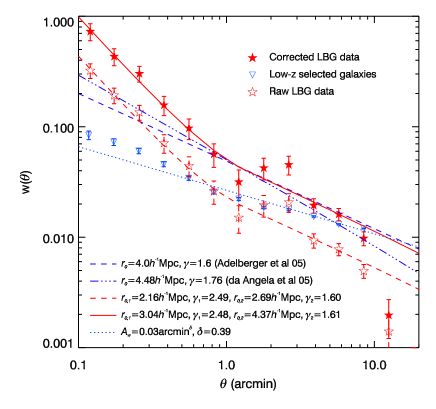
Figure 17: The angular correlation function, $w(\theta)$, from our imaging fields. The open stars show the correlation function for the photometrically selected sample, whilst the filled stars show the same correlation function corrected for stellar and $z<2$ galaxy contamination as described in the text. The dashed red and solid red lines show the double power law models fitted to the raw and contamination corrected correlation functions respectively. We also show a model determined from the $r_{0}$, $\gamma$ measurements of da Ângela et al. (2005a) - dash-dot blue line. The blue triangles and dotted line show the correlation function and best fitting power law model for the photometrically selected $z<2$ galaxy population. The blue dash line gives the result of Adelberger et al. (2005b), with $r_{0}=4.0~{}h^{-1}{\rm Mpc}$ and $\gamma=1.57$.

Additionally we show the correlation function, estimated in the same way, for the remaining $23<R<25.5$ galaxy population (i.e. all galaxies in the given magnitude range not selected by the LBG colour selection - blue triangles). This gives an estimate of the clustering for the $z<2$ galaxy population in the LBG fields. Based on the spectroscopic results, we estimate that $60\%$ of the photometric selection consists of $z>2$ galaxies whilst the remaining $40\%$ consists of contaminant $z<2$ galaxies and galactic stars. In order to determine more accurately the clustering of our selected $z>2$ galaxy population, we therefore correct the $w(\theta)$ measurement for the effects of contamination. The correction is given by:

$$w_{\mathrm{meas}}(\theta)=w_{z<2}(\theta)f_{z<2}^{2}+w_{\mathrm{LBG}}(\theta)f_{\mathrm{LBG}}^{2}$$ (8)

where $w_{\mathrm{meas}}$ is the total measured correlation function, $w_{z<2}(\theta)$ is the correlation function of the contaminant galaxies, $f_{z<2}$ is the fraction of contaminant galaxies, $w_{\mathrm{LBG}}(\theta)$ is the correlation function of the $z>2$ galaxies and $f_{\mathrm{LBG}}$ is the fraction of $z>2$ galaxies. We therefore use the measured correlation function (i.e. open red stars in Fig. 17) and the measured $z<2$ correlation function (i.e. blue triangles in Fig. 17) along with the spectroscopically measured fractions of $z>2$ and $z<2$ galaxies to estimate the $z>2$ galaxy correlation function (i.e. $w_{\mathrm{LBG}}$). The result is shown by the filled red stars in Fig. 17. At all scales we find a higher measurement of the $z>2$ correlation function after applying this correction. We note that the $w_{\mathrm{LBG}}(\theta)$ measurement shows signs of a change in slope at $\theta\sim 0.6-1\arcmin$, suggestive of the combination of one and two halo terms used in Halo Occupation Distribution modeling (HOD, e.g. Abazajian et al. 2005; Zheng et al. 2005; Wake et al. 2008; Zheng et al. 2009).

We now quantify the clustering amplitude of the raw and corrected $w(\theta)$ measurements using a simple power-law fit, with constants $A_{w}$ and $\delta$ such that:

$$w(\theta)=A_{w}\theta^{-\delta}$$ (9)

Fitting to the data to the large scale clustering ($0.8\arcmin<\theta<10\arcmin$) for the uncorrected $w(\theta)$ we obtain best fit parameters of $A_{w}=1.08\pm 0.27\times 10^{-3}\text{deg}^{\delta}$ and $\delta=0.76^{+0.07}_{-0.17}$. Using the same angular range with the corrected $w(\theta)$ gives parameters of $A_{w}=1.85^{+0.41}_{-0.21}\times 10^{-3}\text{deg}^{\delta}$ and $\delta=0.82^{+0.11}_{-0.12}$. We also perform a fit to the $z<2$ correlation function. In this case, the clustering is fit by a power law with $A_{w}=2.31^{+0.58}_{-0.58}\times 10^{-3}\text{deg}^{\delta}$ and $\delta=0.57^{+0.01}_{-0.01}$ (dotted blue line in Fig. 17).

We now estimate the real-space correlation function, $\xi(r)$, from our measurement of $w(\theta)$ using Limber’s formula (Phillipps et al., 1978) with our measured redshift distribution (Fig. 10). This is performed for both the raw $w(\theta)$ and the contamination-corrected $w(\theta)$ with a double power-law form of $\xi(r)$ given by:

$$\xi_{1}=\left(\frac{r_{0,1}}{r}\right)^{-\gamma_{1}}(r<r_{b})$$ (10)

$$\xi_{2}=\left(\frac{r_{0,2}}{r}\right)^{-\gamma_{2}}(r\geq r_{b})$$ (11)

where $r_{b}$ is the break at which the power-law is split between the two power-laws, $r_{0}$ is the clustering length and $\gamma$ is the slope (which is given by $\gamma=1+\delta$). We perform $\chi^{2}$ fitting over the $r_{0}$-$\gamma$ parameter space to both the uncorrected and corrected $w(\theta)$ results. Firstly for the uncorrected result, we find $r_{0,2}=3.14^{+0.17}_{-0.36}~{}h^{-1}{\rm Mpc}$ and $\gamma_{2}=1.81^{+0.09}_{-0.14}$. For the corrected $w(\theta)$, we determine a clustering length above the break of $r_{0,2}=4.37^{+0.43}_{-0.55}~{}h^{-1}{\rm Mpc}$, with a slope of $\gamma_{2}=1.61\pm 0.15$. The full results are given in table 6 and the best-fitting $w(\theta)$ models are plotted in Fig. 17. We note that for continuity in the double power-law function, the break is found to be at $r_{b}\approx 1.5~{}h^{-1}{\rm Mpc}$.

Table 6: Clustering results based on the raw $w(\theta)$ and the $w(\theta)$ corrected for stellar and low-redshift galaxy contamination.

	$A_{w}$	$\delta$	$r_{0,1}$	$\gamma_{1}$	$r_{0,2}$	$\gamma_{2}$
	($\times 10^{-3}$degδ)		($~{}h^{-1}{\rm Mpc}$)		($~{}h^{-1}{\rm Mpc}$)
Uncorrected data	$1.08^{+0.27}_{-0.27}$	$0.76^{+0.07}_{-0.17}$	$2.16^{+0.24}_{-0.30}$	$-2.49^{+0.09}_{-0.12}$	$2.69^{+0.20}_{-0.26}$	$-1.60\pm 0.11$
Contamination-corrected	$1.85^{+0.41}_{-0.21}$	$0.82^{+0.11}_{-0.12}$	$3.04^{+0.33}_{-0.34}$	$-2.48^{+0.10}_{-0.11}$	$4.37^{+0.43}_{-0.55}$	$-1.61\pm 0.15$

Comparing our result to previous results, da Ângela et al. (2005a) obtained a clustering length of $r_{0}=4.48^{+0.09}_{-0.14}~{}h^{-1}{\rm Mpc}$ with a slope of $\gamma=1.76^{+0.08}_{-0.09}$ and Adelberger et al. (2003) obtained $r_{0}=3.96\pm 0.15~{}h^{-1}{\rm Mpc}$ and $\gamma=1.55\pm 0.29$, both using a single power-law function fit ($\xi(r)=(r/r_{0})^{-\gamma}$) to the same $z\approx 3$ LBG data (Steidel et al., 2003). Our sample appears to have a comparable clustering strength, which is slightly higher when corrected for stellar/low-redshift galaxy contamination. A further comparison can be made with the work of Foucaud et al. (2003), who measured an amplitude of $r_{0}=5.9\pm 0.5~{}h^{-1}{\rm Mpc}$ from the $w(\theta)$ of a sample of 1294 $20.0<R_{\mathrm{AB}}<24.5$ LBG candidates in the Canada-France Deep Fields Survey (McCracken et al., 2001). Hildebrandt et al. (2007) measure the clustering of LBGs in the GaBoDS data and find a clustering length of $r_{0}=4.8\pm 0.3~{}h^{-1}{\rm Mpc}$ for a sample of $22.5<R_{\mathrm{Vega}}<25.5$ galaxies. Subsequently to this, Hildebrandt et al. (2009) measured the clustering properties of LBGs selected in the $ugr$ filters from the CFHTLS data and measured a clustering length of $r_{0}=4.25\pm 0.13~{}h^{-1}{\rm Mpc}$ with a magnitude limit of $r_{AB}<25$ and using redshift estimates based on the HYPERZ photometric code (Bolzonella et al., 2000). Our contamination-corrected result appears consistent with most previous work, although lower than the result of Foucaud et al. (2003).

4.1.1 Slit Collisions

After calculating the angular correlation function, we next use the redshift information from our spectroscopic survey in order to confirm the clustering properties of the LBGs. However, before we do this we need to evaluate the extent to which we are limited in observing close-pairs by the VIMOS instrument set up. With the LR_Blue grism, each dispersed spectrum covers a length of 570 pixels on the CCD. Further to this each slit has a length (perpendicular to the dispersion axis) in the range of 40-120 pixels. Given the VIMOS camera pixel scale of 0.205$\arcsec/\textrm{pixel}$, each observed object therefore covers a minimum region of $\approx 120\arcsec\times 8.2\arcsec$, in which no other object can be targeted.

In order to evaluate this effect, we calculate the angular auto-correlation function for only those candidate objects that were targeted in our spectroscopic survey, $w_{slits}(\theta)$. To do so we require a tailored random catalogue that accounts for the geometry of the VIMOS CCD layout. We therefore create random catalogues for each sub-field using a mask based on the layout of the four VIMOS quadrants, excluding any objects that fall within the $2\arcmin$ gaps between adjacent CCDs. The sky-density of randoms in each sub-field is set to be $20\times$ the sky-density of data points in the corresponding parent field. From this subset, which consists of $\approx 3400$ targeted objects, we calculate $w_{slits}(\theta)$ using the Landy-Szalay estimator (equation 4). The ratio of $1+w_{slit}(\theta)$ to the original measurement of $1+w(\theta)$ (prior to correction for contamination) is shown in Fig. 18 (open circles). At $\theta>2\arcmin$ the two correlation functions follow each other closely and give a ratio of $\approx 1$. However at separations of $\theta<2\arcmin$ we see an increasingly significant loss of clustering showing the effect of the instrument setup. At redshifts of $z\approx 3$, the $2\arcmin$ threshold of the effect corresponds to a comoving separation of $r\approx 2.6~{}h^{-1}{\rm Mpc}$.

Figure 18: Effect of ’slit collisions’ on the measurement of the angular correlation function, $w_{\theta}$. We show the ratio between the clustering of the entire photometric sample, given by $1+w(\theta)$, and the clustering measured from only those objects that have been spectroscopically observed using VLT VIMOS, $1+w_{slits}(\theta)$. The observational constraints incurred due to the constraint of preventing the dispersed spectra from overlapping on the instrument CCD lead to a significant reduction in the clustering measurement at $\theta<2\arcmin$. The dashed line shows our parameter fit (equation 12) to the measured ratio, which we use to correct subsequent clustering measurements made using the spectroscopic galaxy sample.

The dashed line in Fig. 18 shows a fit to the ratio between the slit-affected clustering measurement and the original measurement. We use this fit to provide a weighting factor dependent on angular separation, $W_{slit}(\theta)$, which is given by:

$$W_{slit}(\theta)=\frac{1}{1-0.0738\theta^{-1.052}}$$ (12)

Applying this weighting function to DD pairs at separations of $\theta<2\arcmin$ then allows the recovery of the original correlation function from the VIMOS sub-sample correlation function down to separations of $\theta\approx 0.1\arcmin$. Below $\theta\approx 0.1\arcmin$ however we are unable to recreate the original candidate correlation function as no close pairs can be observed below this scale due to the slit lengths ($8\arcsec<\theta<24\arcsec$) used in the VIMOS masks.

4.2 Semi-Projected Correlation Function, $w_{p}(\sigma)$

We next present the semi-projected correlation function $w_{p}(\sigma)$ for the 1020 $q\geq 0.5$ VLT LBGs. Here, $\sigma$ is the transverse separation given by the separation on the sky, whilst $\pi$ will be its orthogonal, line-of-sight component. We first estimate $w_{p}(\sigma)$ for the full VLT LBG sample using (Davis & Peebles, 1983):

$$w_{p}(\sigma)=2\int^{\infty}_{0}\xi(\sigma,\pi)d\pi$$ (13)

We perform the integration over the line of sight range from $\pi=0$ to $100~{}h^{-1}{\rm Mpc}$. This encompasses much of the bulk of the significant signal in the correlation function and performing the calculation over a range of reasonable limits showed the result to be robust. The VLT $w_{p}(\sigma)$ is shown in Fig. 19 with the best fit clustering model determined by a $\chi^{2}$ fit to the data shown as a dotted line. For the projected correlation function a simple power law form of $\xi(r)$ gives:

$$w_{p}(\sigma)/\sigma=r_{0}^{\gamma}\sigma^{-\gamma}\left(\frac{\Gamma\left(\frac{1}{2}\right)\Gamma\left(\frac{\gamma-1}{2}\right)}{\Gamma\left(\frac{\gamma}{2}\right)}\right),$$ (14)

where $\Gamma()$ is the Gamma function. We perform the fit to the data using a fixed value for the slope of the function of $\gamma=1.8$. With this value, we obtain $r_{0}=3.67^{+0.23}_{-0.24}~{}h^{-1}{\rm Mpc}$ for the full VLT sample. Comparing to the initial estimate from the $w(\theta)$ measurement in Fig. 18, we find the $w_{p}(\sigma)$ measurement gives a somewhat lower value for $r_{0}$. The difference is at the $\lesssim 2\sigma$ level and given the level of contamination in the photometric sample, we expect the $w_{p}(\sigma)$ measurement to be the more reliable.

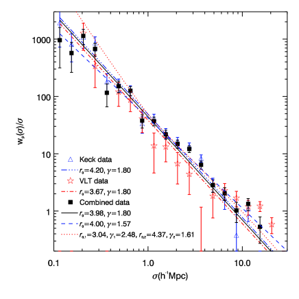
Figure 19: Projected correlation function, $w_{p}(\sigma)$ of the full VLT, Keck (Steidel et al., 2003) and the combined samples. The blue dash-triple-dot line represents our best-fit (with $\gamma=1.8$) to the Keck data of $r_{0}=4.20^{+0.14}_{-0.15}~{}h^{-1}{\rm Mpc}$. The dot-dashed line represents the best $\gamma=1.8$ fit to the VLT sample with $r_{0}=3.67^{+0.23}_{-0.24}~{}h^{-1}{\rm Mpc}$. The solid line represents the best $\gamma=1.8$ fit to the combined VLT$+$Keck sample with $r_{0}=3.98^{+0.23}_{-0.24}~{}h^{-1}{\rm Mpc}$ and the dotted line represents the double-power-law model fitted to the VLT $w(\theta)$. The dashed line gives the result of Adelberger et al. (2005b), with $r_{0}=4.0~{}h^{-1}{\rm Mpc}$ and $\gamma=1.57$.

We next compare the VLT result to the LBG Keck sample of Steidel et al. (2003). This sample consists of 940 LBGs in the redshift range $2.0\lesssim z\lesssim 3.9$, with a mean redshift of $\left<z\right>=2.96\pm 0.29$ (compared to $2.0\lesssim z\lesssim 4.0$ and $\left<z\right>=2.87\pm 0.34$ for the VLT LBG survey). The survey is based on observations within 17 individually observed fields, with most of these being $\approx 8\arcmin\times 8\arcmin$ with a few exceptions (the largest field being $\approx 15\arcmin\times 15\arcmin$). The Keck spectroscopic data covers a total area of $0.38{\rm deg}^{2}$, with just a small number of the fields being adjacent. The median rest-frame UV absolute magnitude is $M_{1700}=-17.92\pm 0.02$, based on the commonly used transformations to $M_{1700}$ using the observed magnitudes ${\cal R}$ and $G$ (e.g. Sawicki & Thompson, 2006; Reddy et al., 2008). With the same method (and the transformations to ${\cal R}$ and $G$ AB magnitudes given by Steidel & Hamilton 1993), we estimate a median rest-frame UV absolute magnitude of $M_{1700}=-18.19\pm 0.03$ for our VLT sample. The samples appear broadly compatible, with the Keck sample having a marginally fainter average absolute magnitude, most likely due to the greater number of fainter objects (${\cal R}\gtrsim 25$) observed with the deeper spectroscopy obtained for the Keck sample.

Combining the two spectroscopic data-sets gives a total of 1,980 LBGs over a total area of $1.56{\rm deg}^{2}$. In Fig. 19 we further present the Keck and combined results for $w_{p}(\sigma)$. The VLT results are slightly lower than for the Keck data in the range $1<\sigma<7~{}h^{-1}{\rm Mpc}$. The result for the combined sample is dominated by Keck pairs for $\sigma<7~{}h^{-1}{\rm Mpc}$ and VLT pairs at larger scales. The solid line represents the $r_{0}=4.20^{+0.14}_{-0.15}~{}h^{-1}{\rm Mpc}$, $\gamma=1.8$ fit for the Keck data. The dashed line represents $r_{0}=3.98^{+0.13}_{-0.12}~{}h^{-1}{\rm Mpc}$, which gives the best $\gamma=1.8$ fit to the VLT$+$Keck combined $w_{p}$ data. Also shown is the best $\gamma=1.8$ fit to the full VLT sample with $r_{0}=3.67^{+0.23}_{-0.24}~{}h^{-1}{\rm Mpc}$.

To calculate $w_{p}(\sigma)$ for the double power-law $\xi(r)$ that we fitted above to the VLT $w(\theta)$ we used the relation

$$w_{p}(\sigma)=2\int_{\sigma}^{\infty}\frac{r\xi(r)}{\sqrt{r^{2}-\sigma^{2}}}dr$$ (15)

The dot-dashed line in Fig. 19 then shows that this model also gives a good fit to the combined $w_{p}(\sigma)$.

4.3 Redshift-Space Correlation Function

The redshift-space correlation function, $\xi(s)$, is an estimator of the clustering of a galaxy population as a function of the redshift-space distance, $s$, which is given by $s=\sqrt{\sigma^{2}+\pi^{2}}$. Now, using the full VLT sample of 1,020 $q\geq 0.5$ spectroscopically confirmed $z>2$ galaxies, we estimate $\xi(s)$ using the simple estimator $\xi(s)=DD(s)/DR(s)-1$. Again the random catalogues were produced individually for each field to match the VIMOS geometry and with $20\times$ the number of objects as in the associated data catalogues. The DD pairs were then corrected for slit collisions using the angular weighting function (equation 12) applied to pairs with separations of $\theta<2\arcmin$. The result is shown in Fig. 20 (filled circles) with Poisson error estimates. The accuracy of these errors is supported by analysis of mock catalogues generated from N-body simulations (da Ângela et al., 2005a; Hoyle et al., 2000). Plotted for comparison is the Keck result as analysed by da Ângela et al. (2005a). Also shown is the combined VLT$+$Keck $\xi(s)$ result.

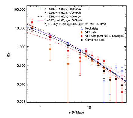
Figure 20: Redshift-space clustering function, $\xi(s)$, calculated from 1020 spectroscopically identified LBGs in the full VLT, Keck and combined samples. Also shown is the result from the 529 LBGs in the high S/N VLT sample. The models generally adopt the $\gamma=1.8$, $\xi(r)$ amplitudes fitted to $w_{p}(\sigma)$. Thus the combined VLT$+$Keck model assumes $r_{0}=3.98~{}h^{-1}{\rm Mpc}$ and expected velocity dispersions of $<w_{z}^{2}>^{1/2}=720~{}{\rm kms}^{-1}$ (VLT) and $<w_{z}^{2}>^{1/2}=400~{}{\rm kms}^{-1}$ (Keck). Also shown is a model with $r_{0}=3.67~{}h^{-1}{\rm Mpc}$ from the full VLT $w_{p}(\sigma)$ result and $<w_{z}^{2}>^{1/2}=1000~{}{\rm kms}^{-1}$, improving the VLT fit. A further model with $r_{0}=4.2~{}h^{-1}{\rm Mpc}$ from the Keck $w_{p}(\sigma)$ gives a good fit to the Keck $\xi(s)$ with $<w_{z}^{2}>^{1/2}=600~{}{\rm kms}^{-1}$. Finally, we show the 2-power-law VLT $w(\theta)$ model, assuming $<w_{z}^{2}>^{1/2}=1000~{}{\rm kms}^{-1}$. All models assume $\beta=0.48$ (see Sect. 4.4.)

The VLT and Keck samples show good agreement at separations of $s>8~{}h^{-1}{\rm Mpc}$, however the VLT sample shows a significant drop in clustering strength at $1<s<8~{}h^{-1}{\rm Mpc}$ compared to the Keck measurement. This seems at odds with the $w(\theta)$ result, which points to the two samples having similar clustering strengths. However, we note that the estimate of the line-of-sight distances is sensitive to any intrinsic peculiar velocities and also errors on the redshift estimate, which will have a consequent effect on the measured redshift space correlation function. In addition to this, the peculiar velocities are an important element in the cross-correlation between the galaxy population and the Ly$\alpha$forest, which is presented with this galaxy sample in Crighton et al. (2010). We therefore now estimate the effect of our redshift errors on this result. The error on a given LBG redshift is a combination of the mean error on the spectral feature measurements, which is given by the measurement error on the Ly$\alpha$ emission line from Fig. 7, (i.e. $\approx\pm 450~{}{\rm kms}^{-1}$ given average spectral S/N=5.5 in the full VLT sample) combined with the error on the estimation of the redshift from the measurement of the outflow features ($\approx\pm 200~{}{\rm kms}^{-1}$). In addition, there will be some contribution from intrinsic peculiar velocities. We estimate this contribution based on the work of (Tummuangpak et al., In prep). Tummuangpak et al. (In prep) use the Galaxies-Intergalactic Medium Interactions Calculation (GIMIC, Crain et al., 2009), which samples a number of sub-grids of the Millennium Simulation Springel et al. (2005), populating these with baryons using hydrodynamic simulations. Tummuangpak et al. (In prep) measure a mean intrinsic peculiar velocity based on galaxies in the GIMIC simulations in redshift slices at $z=3.06$ and find a value of $\approx 140~{}{\rm kms}^{-1}$. Combining this in quadrature with the estimated measurement errors gives an overall velocity dispersion of $\sigma_{z}=\sqrt{(450~{}{\rm kms}^{-1})^{2}+(200~{}{\rm kms}^{-1})^{2}+(140~{}{\rm kms}^{-1})^{2}}\approx 510~{}{\rm kms}^{-1}$. The expected overall VLT pairwise velocity dispersion is therefore $<w_{z}^{2}>^{1/2}=\sqrt{2}\times 510\approx 720~{}{\rm kms}^{-1}$. Substituting a Ly$\alpha$ emission-line velocity error of $\pm 150~{}{\rm kms}^{-1}$ (based on a measurement error of $\Delta z\approx 0.002$ from Steidel et al., 2003) in the above expression similarly implies an expected $<w_{z}^{2}>^{1/2}\approx 400~{}{\rm kms}^{-1}$ for the Keck pairwise velocity dispersion.

On small scales, the above random pair-wise velocity dispersion leads to the well known ‘finger-of-god’ effect on redshift-space maps and correlation functions. On larger scales, bulk infall motion towards over-dense regions becomes a significant factor and causes a flattening in the line-of-sight direction in redshift space. We now model these two effects to see if the $\xi(r)$ estimates measured from the LBG semi-projected correlation function, $w_{p}(\sigma)$, and the angular correlation function, $w(\theta)$, are consistent with the measured LBG redshift-space correlation function, $\xi(s)$. Following Hawkins et al. (2003), we use the real-space prescription for the large scale infall effects given by Hamilton (1992) whereby the 2-D infall affected correlation function is given by:

$$\xi^{\prime}(\sigma,\pi)=\xi_{0}(s)P_{0}(\mu)+\xi_{2}(s)P_{2}(\mu)+\xi_{4}(s)P_{4}(\mu)$$ (16)

where $P_{l}(\mu)$ are Legendre polynomials, $\mu=cos(\theta)$ and $\theta$ is the angle between $r$ and $\pi$. For a simple power-law form of $\xi(r)$ the forms of $\xi_{l}(s)$ are:

$$\xi_{0}(s)=\left(1+\frac{2\beta}{3}+\frac{\beta^{2}}{5}\right)\xi(r)$$ (17)

$$\xi_{2}(s)=\left(\frac{4\beta}{3}+\frac{4\beta^{2}}{7}\right)\left(\frac{\gamma}{\gamma-3}\right)\xi(r)$$ (18)

$$\xi_{4}(s)=\frac{8\beta^{2}}{35}\left(\frac{\gamma(2+\gamma)}{(3-\gamma)(5-\gamma)}\right)\xi(r)$$ (19)

where $\gamma$ is the slope of the power-law form of the real-space correlation function: $\xi(r)=(r/r_{0})^{-\gamma}$. For the 2-power-law model case we use the equivalent expressions derived by da Ângela et al. (2005a). As in Hawkins et al. (2003), the infall affected clustering, $\xi^{\prime}(\sigma,\pi)$ is then convolved with the random motion (in this case the pair-wise motion combined with the measurement uncertainties):

$$\xi(\sigma,\pi)=\int_{-\infty}^{\infty}\xi^{\prime}(\sigma,\pi-v(1+z)/H(z))f(v)dv$$ (20)

where $H(z)$ is Hubble’s constant at a given redshift, $z$, and $f(v)$ is the profile of the random velocities, $v$, for which we use a Gaussian with width equal to the pair-wise velocity dispersion, $<w_{z}^{2}>^{1/2}$.

With this form of $f(v)$, we take the expected pair-wise velocity dispersion, $<w_{z}^{2}>^{1/2}=720~{}{\rm kms}^{-1}$ for the full VLT sample and $<w_{z}^{2}>^{1/2}=400~{}{\rm kms}^{-1}$ for the Keck sample. Now taking an estimate of $\beta=0.48$ (see Section 4.4), we may model the effect of these velocity components on the LBG sample $\xi(\sigma,\pi)$, first using the single power-law fit to the combined sample $w_{p}(\sigma)$ with $r_{0}=3.98~{}h^{-1}{\rm Mpc}$ and $\gamma=1.8$. The form of $\xi(s)$ estimated from the resultant $\xi(\sigma,\pi)$ is plotted in Fig. 20 (solid line). While the model with $<w_{z}^{2}>^{1/2}=400~{}{\rm kms}^{-1}$ gives a good fit to the Keck data, the model with $<w_{z}^{2}>^{1/2}=720~{}{\rm kms}^{-1}$ appears to overestimate the VLT correlation function at $s<8~{}h^{-1}{\rm Mpc}$. Even increasing the velocity dispersion to $1000~{}{\rm kms}^{-1}$ did not significantly improve the fit. We also analysed the LBG sub-sample defined by having spectral $S/N>5$. We found that $\xi(s)$ for this subsample did rise and would require a pair-wise velocity dispersion of $\approx 1000~{}{\rm kms}^{-1}$ for the model to fit the data. This is significantly more than the predicted pair-wise velocity dispersion of $\approx 600~{}{\rm kms}^{-1}$, calculated by replacing the velocity error of $450~{}{\rm kms}^{-1}$ for the full sample by $350~{}{\rm kms}^{-1}$ in this case, corresponding to average S/N=8.25 in Fig. 7. The fact that the points at $s<1~{}h^{-1}{\rm Mpc}$ and those at $s>8~{}h^{-1}{\rm Mpc}$ agree with the model argues against an even larger velocity dispersion.

The other possibility is that the $r_{0}=3.98~{}h^{-1}{\rm Mpc}$ model may be too high for the VLT $\xi(r)$. Certainly the amplitude of $\xi(r)$ from the VLT $w_{p}(\sigma)$ appears lower than either that from the VLT $w(\theta)$ or the Keck $w_{p}(\sigma)$. Fig. 20 shows that the fit improves for the full VLT samples and the high S/N subsample if the correlation function amplitude reduces to $r_{0}=3.67~{}h^{-1}{\rm Mpc}$ as fitted to the VLT $w_{p}(\sigma)$, coupled with the velocity dispersion increasing to $<w_{z}^{2}>^{1/2}=1000~{}{\rm kms}^{-1}$.

The combined VLT$+$Keck sample is very similar to the Keck sample at small scales. Even for the Keck sample we find that an increased pairwise velocity dispersion of $<w_{z}^{2}>^{1/2}\approx 600~{}{\rm kms}^{-1}$ is needed to fit $\xi(s)$ if $r_{0}=4.2~{}h^{-1}{\rm Mpc}$. For the Keck LBGs, the velocity error ($\pm 150~{}{\rm kms}^{-1}$, Steidel et al. 2003) $+$ intrinsic outflow error ($\pm 200~{}{\rm kms}^{-1}$, Adelberger et al. 2003) combines in quadrature to give $\pm 250~{}{\rm kms}^{-1}$ as the error for the line measurement. Subtracting from $\pm 600/\sqrt{2}~{}{\rm kms}^{-1}$ would imply $\approx 340~{}{\rm kms}^{-1}$ for the pairwise intrinsic velocity dispersion. Clearly for the VLT samples the implied velocity dispersion would be even larger.

We have also used the double power-law $\xi(r)$ indicated by the VLT $w(\theta)$ to predict $\xi(s)$. Since the steepening takes place at $r<3~{}h^{-1}{\rm Mpc}$, this means that we would need even higher velocity dispersions to fit $\xi(s)$. Fig. 20 shows that the double power-law model needs at least a velocity dispersion of $\approx 1000~{}{\rm kms}^{-1}$ to fit the VLT$+$Keck combined sample.

We conclude that the low $\xi(s)$ we find in the full VLT sample may be caused by a statistical fluctuation in the LBG clustering due to a lower than average $r_{0}$ and a higher than average velocity dispersion. The VLT sample is designed to improve correlation function accuracy at large scales, particularly in the angular direction, and the somewhat noisy result for $\xi(s)$ at the smallest scales reflects this. Overall, we conclude that the velocity dispersions required by $\xi(s)$ are bigger than reported previously for the Keck data ($400~{}{\rm kms}^{-1}$ by da Ângela et al., 2005a) with the Keck and VLT samples now being fitted by $<w_{z}^{2}>^{1/2}=600-1000~{}{\rm kms}^{-1}$, close to what is expected from estimates of the redshift errors.

4.4 Estimating the LBG infall parameter, $\beta(z=3)$

The infall parameter, $\beta$, quantifies the extent of large scale coherent infall towards overdense regions via the imprint of the infall motion on the observed redshift space distortions. Given its dependence on the distribution of matter, measuring $\beta$ can provide a useful dynamical constraint on $\Omega_{m}(z)$ (Hamilton, 1992; Heavens & Taylor, 1995; Hawkins et al., 2003; da Ângela et al., 2008; Cabré & Gaztañaga, 2009). It relates the real-space clustering and redshift-space clustering as outlined in the previous section (see equations 16 to 19).

We shall measure $\beta(z=3)$, using the combination of our VLT LBG data and the LBG data of Steidel et al. (2003). As noted above, the VLT and Keck samples complement each other in the wide range of separation, $\sigma$, in the angular direction for the VLT sample and the high sky densities of the Keck samples, which help define the clustering better at small scales. As discussed in section 4.3, the two samples possess comparable real-space clustering strengths, with measured clustering lengths of $r_{0}=3.67^{+0.23}_{-0.24}~{}h^{-1}{\rm Mpc}$ and $r_{0}=4.20^{+0.14}_{-0.15}~{}h^{-1}{\rm Mpc}$ for the VLT and Keck LBG samples respectively. The higher estimated velocity error of the VLT sample at $\pm 450~{}{\rm kms}^{-1}$ compared to the Keck $\pm 300~{}{\rm kms}^{-1}$ will make little difference due to the further contributions of the outflow errors and intrinsic velocity dispersions, the dominance of the Keck data at small scales and the smaller effect of velocity errors at large spatial scales where the VLT data is dominant. We shall therefore combine the two samples in the two methods we use to measure $\beta$.

We first estimate $\beta$ by simply comparing the amplitude of $\xi(s)$ and $\xi(r)$ and using equation 17 at large scales. Fig. 21 shows the $\xi(s)$ from the combined VLT and Keck samples divided by the best fit model for $\xi(r)$ from the semi-projected correlation function, $w_{p}(\sigma)$, with $r_{0}=3.98^{+0.13}_{-0.12}~{}h^{-1}{\rm Mpc}$ and $\gamma=1.8$. Equation 17 applies only in the linear regime, so we do not expect it to fit at small separations. We therefore fit at $s>10~{}h^{-1}{\rm Mpc}$. Fitting in the ranges $10<s<25~{}h^{-1}{\rm Mpc}$ and $10<s<60~{}h^{-1}{\rm Mpc}$ gives the two dashed lines in Fig. 21, which correspond to $\beta(z=3)=0.51^{+0.20}_{-0.23}$ and $\beta(z=3)=0.38^{+0.19}_{-0.23}$ with the difference between these two giving a further estimate of the uncertainty in $\beta$ from this method.

Figure 21: The redshift space correlation function, $\xi(s)$ divided by the real space correlation function, $\xi(r)$, with the latter assuming $r_{0}=3.98~{}h^{-1}{\rm Mpc}$ and $\gamma=1.8$. The short and long dashed lines represent the best fit to the data in the ranges $10<s<25~{}h^{-1}{\rm Mpc}$ and $10<s<60~{}h^{-1}{\rm Mpc}$, which correspond to $\beta(z=3)=0.51^{+0.20}_{-0.23}$ and $\beta(z=3)=0.38^{+0.19}_{-0.23}$ from equation 17.

We next estimate $\beta$ using the shape of the 2-point correlation function, $\xi(\sigma,\pi)$, to measure the effect of redshift space distortions. We calculate $\xi(\sigma,\pi)$ for the combined sample. As with our determination of $\xi(s)$, we use the simple $DD/DR$ estimator taking randoms tailored to each individual field, with errors again calculated using the Poisson estimate. The resultant $\xi(\sigma,\pi)$ is plotted in Fig. 22. The elongation in the $\pi$ dimension, due to the pair-wise velocity dispersion and redshift errors, is clearly evident at small scales.

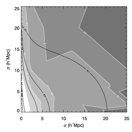
Figure 22: $\xi(\sigma,\pi)$ projected correlation function calculated from the spectroscopically confirmed LBGs from the combined Steidel et al. (2003) and VLT VIMOS LBG samples. The best fit model contours are marked as solid lines with $\beta(z=3)=0.48$ and $<w_{z}^{2}>^{1/2}=700~{}{\rm kms}^{-1}$.

Now using this measurement of $\xi(\sigma,\pi)$, we make an estimate of the infall parameter, $\beta$. For this we use the single power-law model of $\xi(r)$ with $r_{0}=3.98~{}h^{-1}{\rm Mpc}$ and $\gamma=1.8$ based on the semi-projected correlation function of the combined data in Fig. 19. With these parameters set, we calculate the model outlined in equations 16 to 20 over a range of values of $<w_{z}^{2}>^{1/2}$ and $\beta$. We then perform a simple $\Delta\chi^{2}$ fitting analysis and jointly estimate $<w_{z}^{2}>^{1/2}=700\pm 100~{}{\rm kms}^{-1}$ and infall parameter of $\beta_{\mathrm{LBG}}(z\approx 3)=0.48\pm 0.17$ for our combined LBG sample. The contour plot of $\Delta\chi^{2}$ for the fit in the $<w_{z}^{2}>^{1/2}:\beta$ plane is given in Fig. 23.

We note that if we allow the amplitude of $\xi(r)$ to be fitted as well as the other two parameters, then the results move to $\beta=1.1\pm 0.4$ and $<w_{z}^{2}>^{1/2}=800\pm 100~{}{\rm kms}^{-1}$ for a best fit $\gamma=1.8$ value of $r_{0}=3.64~{}h^{-1}{\rm Mpc}$. Taking the Keck sample on its own, we again find $\beta=0.9-1.5$ and $<w_{z}^{2}>^{1/2}=650-750~{}{\rm kms}^{-1}$ if $r_{0}$ is not or is allowed to float respectively. The Keck fits have to be resticted to $s<25~{}h^{-1}{\rm Mpc}$ because of the small $\sigma$ range in the angular direction and if we apply the same cut to the combined sample, values of $\beta$ again rise to $\beta=0.8-1.1$ and $<w_{z}^{2}>^{1/2}\approx 800~{}{\rm kms}^{-1}$, similar to the results for the Keck sample. Although the errors are clearly still significant, we prefer values of $\beta\approx 0.5-0.6$ given by the amplitude of $\xi(s)$ and the shape of $\xi(\sigma,\pi)$ for the combined sample which seems best to exploit the advantages of the Keck sample at small scales and the VLT sample at large scales.

We have also checked the effect of assuming the double power-law model fitted to the LBG $w(\theta)$ in Fig. 17 with $r_{0,1}=3.19~{}h^{-1}{\rm Mpc}$, $\gamma_{1}=2.45$, $r_{0,2}=4.37~{}h^{-1}{\rm Mpc}$, $\gamma_{2}=1.61$ and $r_{b}=1~{}h^{-1}{\rm Mpc}$. The best $\xi(\sigma,\pi)$ fits are then given by $\beta=0.20\pm 0.2$ and $<w_{z}^{2}>^{1/2}=750\pm 150~{}{\rm kms}^{-1}$. The reduced $\chi^{2}$ was 3.44 compared to 3.16 for the single power-law model. However, allowing the $\xi(r)$ amplitude to vary gave $\beta=0.48^{+0.24}_{-0.33}$ and $<w_{z}^{2}>^{1/2}=725^{+175}_{-150}~{}{\rm kms}^{-1}$ with fitted amplitudes $\approx 80$% below those estimated from $w(\theta)$. The small scale rise at $r<1~{}h^{-1}{\rm Mpc}$ will not affect our fit much because of the lack of statistical power at small separations. Also, the models we are using are expected to be accurate only in the linear regime at larger scales. The 80% reduction of the amplitude to the large scale power-law implies an $r_{0}=4.05~{}h^{-1}{\rm Mpc}$ which is close to the $r_{0}=3.98~{}h^{-1}{\rm Mpc}$ value assumed for our single power-law fits above, leading to similar fitted values for $\beta$ and $<w_{z}^{2}>^{1/2}$ in these two cases. The lower $\beta$ from the actual 2 power-law model is simply a result of the high $\xi(r)$ amplitude implied by $w(\theta)$ forcing $\beta$ down in the $\xi(\sigma,\pi)$ fit according to equation 17.

Comparing our result of $\beta=0.48\pm 0.17$ to previous estimates of $\beta(z\sim 3)$, we generally find somewhat higher values than da Ângela et al. (2005a), who estimate a value of $\beta=0.15^{+0.20}_{-0.15}$. This is partly because we have assumed $\Omega_{m}(z=0)=0.3$ and fitted for the velocity dispersion $<w_{z}^{2}>^{1/2}$ whereas da Ângela et al. (2005a) assumed $<w_{z}^{2}>^{1/2}=400~{}{\rm kms}^{-1}$ and fitted for $\Omega_{m}(z=0)$. If we assume $<w_{z}^{2}>^{1/2}=400~{}{\rm kms}^{-1}$ for the VLT $+$ Keck samples, our estimate of $\beta$ reduces to $\beta=0.18$ for the combined sample. The assumption of $<w_{z}^{2}>^{1/2}=400~{}{\rm kms}^{-1}$ seems to be the main factor that drove $\beta$ to lower values, also helped by the different model for $\xi(r)$ assumed by da Ângela et al. (2005a), a 2-power law model with $\gamma_{1}=1.3$ and $\gamma_{2}=3.29$ with $r_{b}=9~{}h^{-1}{\rm Mpc}$ motivated by fitting the form of $\xi(s)$. The contours in the $<w_{z}^{2}>^{1/2}:\beta$ plane in Fig. 23 show that $\beta$ and $<w_{z}^{2}>^{1/2}$ are degenerate - higher $\beta$ implies more flattening in the $\pi$ direction which can be counteracted by fitting a higher $<w_{z}^{2}>^{1/2}$ to produce elongation in $\pi$. A flatter small scale slope for $\xi(r)$ also allows a smaller $<w_{z}^{2}>^{1/2}$ to be fitted which can then allow lower values of $\beta$ to be fitted. We have also fitted our combined data with a further 2-power-law form for $\xi(r)$, now with $r_{0,1}=3.98~{}h^{-1}{\rm Mpc}$, $\gamma_{1}=1.8$, $r_{0,2}=5.99~{}h^{-1}{\rm Mpc}$, $\gamma_{2}=2.6$ and $r_{b}=15~{}h^{-1}{\rm Mpc}$ but we find that the results for $<w_{z}^{2}>^{1/2}$ and $\beta$ from the combined sample are similar to those for the single power-law model.

As well as the higher value of $\beta$, we note that we are also fitting higher velocity dispersion values to the combined sample. Again the degeneracy between $<w_{z}^{2}>^{1/2}$ and $\beta$ may be the cause. However, the need for high velocity dispersions was also noted in the small scale fits to $\xi(s)$ particularly for the VLT sample but also for the Keck sample. Even $<w_{z}^{2}>^{1/2}=600~{}{\rm kms}^{-1}$ for the Keck sample implies an intrinsic velocity dispersion of $<w_{z}^{2}>^{1/2}\approx 440~{}{\rm kms}^{-1}$ taking into account velocity and outflow errors on the redshift, much higher than $<w_{z}^{2}>^{1/2}=200~{}{\rm kms}^{-1}$ expected from the simulations. If our velocity errors were underestimated then this could be a cause but they would have to be underestimated in both the Keck and VLT datasets. Larger velocity errors are also contradicted by the consistent widths of the emission-absorption difference histograms in Fig. 14. For example, assuming $\pm 450~{}{\rm kms}^{-1}$ for the VLT emission velocity error is consistent with $\pm 200~{}{\rm kms}^{-1}$ for the outflow error and $\pm 130~{}{\rm kms}^{-1}$ for the absorption line error.

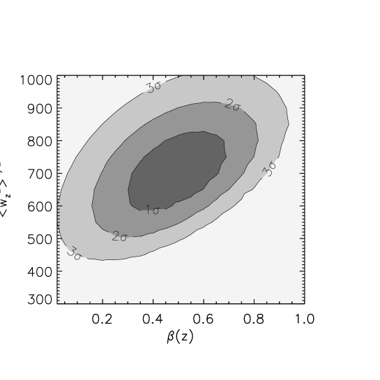
Figure 23: LBG pairwise velocity dispersion ($<w_{z}^{2}>^{1/2}$)-infall parameter($\beta$) $\Delta\chi^{2}$ contours for the VLT$+$Keck sample, fitting to $\xi(\sigma,\pi)$ with $s<40~{}h^{-1}{\rm Mpc}$. The best fit values are $\beta=0.48\pm 0.17$ and $<w_{z}^{2}>^{1/2}=700\pm 100~{}{\rm kms}^{-1}$, assuming $r_{0}=3.98~{}h^{-1}{\rm Mpc}$ and $\gamma=1.8$.

We conclude that for $\Omega_{m}(z=0)=0.3$, the combined survey is best fitted by $<w_{z}^{2}>^{1/2}=700\pm 100~{}{\rm kms}^{-1}$ with $\beta=0.48\pm 0.17$ for a single power-law model with $\gamma=1.8$ and $r_{0}=3.98~{}h^{-1}{\rm Mpc}$. Based on the $\beta=0.49\pm 0.09$ value, $r_{0}=5.05~{}h^{-1}{\rm Mpc}$ and $\gamma=1.8$ values found for 2dFGRS (Hawkins et al., 2003) linear theory predicts $\beta(z=3)=0.22$ in the $\Omega_{m}=1$ case and $\beta=0.37$ in the $\Omega_{m}(z=0)=0.3$ case, with $r_{0}=3.98~{}h^{-1}{\rm Mpc}$ for the latter and transformed appropriately for $\Omega_{m}=1$. Our measurements appear to produce values of $\beta$ that are marginally more acceptable with $\Omega_{m}(0)=0.3$ than $\Omega_{m}(0)=1$ but neither case is rejected at high significance; $\beta=0.22$ with $<w_{z}^{2}>^{1/2}=600~{}{\rm kms}^{-1}$ is rejected only at $1.5\sigma$ in Fig. 23. More importantly, these measurements provide a useful check of the impact of small- and large-scale dynamics on our measurement of the clustering of our $z\approx 3$ galaxies. The estimates of $<w_{z}^{2}>^{1/2}$ will also be useful in interpreting the effect of star-formation feedback from our LBGs on the IGM as measured by the Lyman-alpha forest in background QSOs (Crighton et al., 2010).

4.5 Estimating the LBG bias parameter, $b(z=3)$

We can now estimate the bias, $b$, of the VLT$+$Keck LBG sample from our $\beta$ measurements. The bias gives the relationship between the galaxy clustering and the underlying dark matter clustering:

$$\overset{\_}{\xi}_{g}=b^{2}\overset{\_}{\xi}_{DM}$$ (21)

where $\overset{\_}{\xi}_{DM}$ is the volume averaged clustering of the dark matter distribution and $\overset{\_}{\xi}_{g}$ is the volume averaged clustering of a given galaxy distribution. In a spatially flat universe, the relationship between the bias, $b$, and the infall parameter, $\beta$, can be approximated by (Lahav et al., 1991):

$$\beta=\frac{\Omega_{m}^{0.6}}{b}$$ (22)

Using this relation with our estimate of $\beta=0.48\pm 0.17$ and assuming that $\Omega_{m}(z=0)=0.3$ and then given that $\Omega_{m}(z=3)=0.98$, this implies $b(z=3)=2.06^{+1.12}_{-0.53}$.

We now compare this to an estimate of the bias from our earlier clustering analysis using equation 21. To do this we calculate the dark matter clustering using the CAMB software incorporating the HALOFIT model of non-linearities (Smith et al., 2003). From this we determine a second estimate of the bias using equation 21 and calculating the volume averaged clustering function (Peebles, 1980) within a radius, x, for our galaxy sample and the dark matter:

$$\overset{\_}{\xi}(x)=\frac{3}{x^{3}}\int_{0}^{x}r^{2}\xi(r)dr$$ (23)

where $\xi(r)$ is the 2-point clustering function as a function of separation, $r$. We use an integration limit of $x=20~{}h^{-1}{\rm Mpc}$, ensuring a significant signal, whilst still being dominated by linear scales. Taking the volume averaged non-linear matter clustering, with the volume averaged clustering of our galaxy sample (with $r_{0}=3.98~{}h^{-1}{\rm Mpc}$ and $\gamma=1.8$, from the VLT$+$Keck $w_{p}(\sigma)$ measurement) and determining the bias using equation 21, we find $b=2.22\pm 0.16$, consistent with the estimate from the bulk flow measurement of $\beta=0.48\pm 0.17$ which implies $b=2.06^{+1.12}_{-0.53}$. Both values are somewhat lower than the measurement of the bias of a sample of LBGs from the Canada-France Deep Survey by Foucaud et al. (2003) who measured a value of $b=3.5\pm 0.3$.

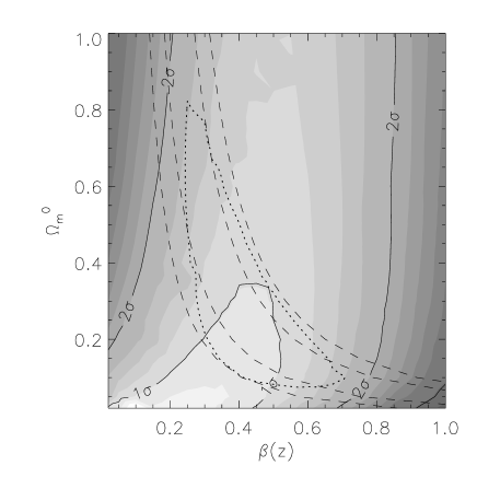
Figure 24: The shaded regions are the $\Omega_{m}^{0}$-$\beta(z)$ contours for the VLT$+$Keck sample, fitting to $\xi(\sigma,\pi)$ with $s<40~{}h^{-1}{\rm Mpc}$. The dashed lines are the 1- and 2-$\sigma$ contours from comparing the $z\approx 3$ LBG and the 2dFGRS $z\approx 0.1$ clustering amplitudes and also using the 2dFGRS $\beta(z\approx 0.1)=0.49\pm 0.09$ result. The dotted line is the $1-\sigma$ joint contour from applying both of these constraints.

We now estimate the mass of typical host haloes for the $z\approx 3$ LBG sample using the Sheth et al. (2001) prescription for the relation between halo mass and bias, determining a host halo mass of $M_{DM}=\times 10^{11.1\pm 0.1}h^{-1}\rm{M_{\odot}}$. Comparing this to other LBG samples, Foucaud et al. (2003), Hildebrandt et al. (2007) and Yoshida et al. (2008) measure halo masses of bright $z\approx 3$ LBG samples of $M_{DM}\sim 10^{12}h^{-1}\rm{M_{\odot}}$. This difference in mass estimates reflects the deeper magnitude limits of our survey compared to a number of the above results and also a slightly lower redshift range that contribute to our LBG selection sampling a lower mass range. Work using the Steidel et al. (2003, 2004) data, which is closer to our own in redshift and depth, report halo masses of $M_{DM}\sim 10^{11.5}h^{-1}\rm{M_{\odot}}$ (Adelberger et al., 2005b; Conroy et al., 2008), which is closer to the estimate presented here, although our result is still somewhat low.

4.6 Further test of the standard cosmology

Following the analysis of da Ângela et al. (2005a) we can make a further test of the standard cosmology by directly comparing the independent values of the bias from the z-space distortion and the LBG clustering amplitude. Whereas in the above case we assumed the DM clustering for the standard model, here we simply assume the 2dFGRS clustering scale length which we approximate as $r_{0}=5.0~{}h^{-1}{\rm Mpc}$ and $\gamma=1.8$. We also assume their value of $\beta(z\approx 0.1)=0.49\pm 0.09$ from redshift space distortions. In similar fashion to da Ângela et al. (2005a) we can then for any $\Omega_{m}^{0}$, find the mass clustering amplitude at $z=3$ and then we can find the LBG bias, $b(z=3)$, by comparing this to the amplitude of LBG clustering given by $r_{0}=3.98~{}h^{-1}{\rm Mpc}$ and $\gamma=1.8$. This can then be converted to $\beta(z=3)$ by using the value for $\Omega_{m}(z=3)$ implied by the assumed $\Omega_{m}^{0}$ and therefore the $\beta(z):\Omega_{m}^{0}$ relation can be drawn. The 1- and 2-$\sigma$ upper and lower limits on this relation are shown in Fig. 24. These are overlaid on the $\Delta\chi^{2}$ contours (greyscale) from a similar redshift-space distortion analysis as seen in Fig. 23 but now allowing $\Omega_{m}^{0}$ and $\beta(z=3)$ to vary while keeping $<w_{z}^{2}>^{1/2}=700~{}{\rm kms}^{-1}$ constant. In this case we have also allowed the LBG clustering amplitude to be fitted within a 50% range; this is to ensure that the dynamical constraint is as independent as possible of the other constraint which is directly taken from the LBG clustering amplitude. We see that although the best fit from redshift-space distortions has now moved to lower $\Omega_{m}^{0}$ and lower $\beta(z=3)$, there is still a good overlap between the $\pm 1-\sigma$ regions of both constraints. The $1-\sigma$ joint contours from both constraints are shown by the dotted line with the best joint-fit being $\Omega_{m}^{0}=0.2$ and $\beta(z=3)=0.45$. Thus there is certainly no inconsistency with the standard $\Lambda$CDM model although, as before, the $\Omega_{m}^{0}=1$ model is still rejected at less than the $2\sigma$ level. With the values of $\Omega_{m}^{0}$ in a reasonable range, there appears no inconsistency with the evolution of gravitational growth rates as predicted by Einstein gravity, extending the results presented by Guzzo et al. (2008) to $z\approx 3$.

4.7 Clustering Evolution

The space density and clustering evolution of LBGs have frequently been used to infer their descendant galaxy populations at the present day. Initially, their relatively high clustering amplitudes were taken to mean that they would evolve on standard halo models into luminous red galaxies in the richest galaxy clusters at $z=0$ (Steidel et al., 1996; Governato et al., 1998; Adelberger et al., 2005b). On the other hand, Metcalfe et al. (1996, 2001) noted that the comoving density of LBGs was close to that of local spirals. Indeed, they showed that a simple, Bruzual & Charlot (1996), pure luminosity evolution model with e-folding time, $\tau=9$Gyr, plus a small amount of dust, could explain the LBG luminosity function at $z\approx 3$. Recently, more detailed merger tree models have been used to interpret LBG space densities and clustering. For example, Conroy et al. (2008) have concluded on this basis that the descendants are varied, with LBGs evolving to become both blue and red $L^{*}$ and sub-$L^{*}$ galaxies.

We now qualitatively compare the clustering strength of our LBG samples to that of lower redshift galaxies. We first determine the volume-averaged correlation function at $20~{}h^{-1}{\rm Mpc}$ using the single power-law form of the clustering of both our own and the Keck LBG sample as prescribed in equation 23. The $\overset{\_}{\xi}(20)$ measured for the VLT LBG sample is shown in Fig. 25, compared to a number of measures of the clustering of other galaxy samples across a range of redshifts. The VLT$+$Keck result ($r_{0}=3.98~{}h^{-1}{\rm Mpc}$, $\gamma=1.8$, $z=2.87$) is shown by the filled star. We also show the measure for the Keck LBG sample alone (open star) and the Foucaud et al. (2003) LBG sample (cross). The apparent $B$-band magnitude range of the VLT$+$Keck sample is $B=25.69\pm 0.76$. Using the overall redshift range of the sample ($z=2.87\pm 0.34$) and K$+$e corrections determined using the Bruzual & Charlot (2003) stellar population evolution, this equates to an absolute $B$-band magnitude of $M_{B}\approx-21.5\pm 1.1$.

For comparison with our data, we have also plotted the estimated volume-averaged correlation function values for a number of low and high redshift galaxy samples. The open and filled red triangles show the LRG samples of Sawangwit et al. (2009), giving the clustering for a $2L^{*}$ and $3L^{*}$ sample respectively (and having absolute i-band magnitudes of $M_{i(AB)}=-22.4\pm 0.5$ and $M_{i(AB)}=-22.6\pm 0.4$). The open squares show the clustering of late-type galaxies from the 2dFGRS as given by Norberg et al. (2002) with the individual points giving the clustering of galaxies in the absolute magnitude ranges of $-18>M_{bj}>-19$, $-19>M_{bj}>-20$, $-20>M_{bj}>-21$ and $-20.5>M_{bj}>-21.5$ (in order of lowest to highest clustering data-points). In addition we plot the blue spiral galaxies of Bielby et al. (2010) with the open upside-down triangles and Blake et al. (2010) with filled upside-down triangles, plus the sBzKs (open blue diamond) of Hayashi et al. (2007).

As an illustration of how we may expect the clustering of the samples to evolve with time, we first consider a model based on the simulated merger history of dark matter haloes (dot-dot-dot-dash line) calculated from the simulations of González & Padilla (2010), whilst the method used to follow the merger trees is described in Padilla et al. (2010). The simulation was performed using parameter values of $\Omega_{m}=0.26$, $\Omega_{\Lambda}=0.74$, $\sigma_{8}=0.80$ and $n_{s}=1.0$ and consisted of a box size of $L_{box}=123~{}h^{-1}{\rm Mpc}$ containing $512^{3}$ particles with a particle mass of $10^{9}h^{-1}\rm{M_{\odot}}$. The normalization to the LBG data was performed by finding the halo mass ($10^{11.12\pm 0.08}h^{-1}\rm{M_{\odot}}$) for which the halo $\overset{\_}{\xi}_{20}$ matches the $\overset{\_}{\xi}_{20}$ measurement for the VLT LBG sample at its mean redshift. We see that the model predicts little change in the clustering amplitude at $z=1$ and then stronger evolution to a higher clustering amplitude at $z=0$. The amplitude of the clustering at z=0 appears consistent with that of late-type galaxies in the 2dFGRS survey (Norberg et al., 2002). The predicted descendant number density at $z=0$ based on the halo merger tree model is $\mbox{log}_{10}(n/(h^{3}\mbox{Mpc}^{-3}))=-3.49_{-0.51}^{+0.59}$ and is also consistent with number density of the Norberg et al. (2002) $-20.5>M_{bj}>-21.5$ late-type population, which is equal to $\mbox{log}_{10}(n/(h^{3}\mbox{Mpc}^{-3}))=-3.64_{-0.01}^{+0.01}$. These models are able to estimate the transition scale between the 1-halo and 2-halo terms in the correlation function of $0.71^{+1.80}_{-0.51}~{}h^{-1}{\rm Mpc}$, consistent with the transition scale of $r_{b}\approx 1.5\pm 0.3~{}h^{-1}{\rm Mpc}$ in our measured LBG $w(\theta)$. Overall, these conclusions are not dissimilar to those of Conroy et al. (2008). However, Conroy et al. (2008) predicted higher clustering amplitudes, $r_{0}\approx 5-6$h^-1Mpc or $\overset{\_}{\xi}(20)=0.21-0.29$, at $z\approx 1$ and $r_{0}\approx 6-7$h^-1Mpc or $\overset{\_}{\xi}(20)=0.29-0.38$, at $z\approx 0$ for the LBG descendants. Given these differences between the merger-tree models of Padilla et al. (2010) and Conroy et al. (2008), we conclude the results appear somewhat model dependent.

We next compare the $\overset{\_}{\xi}(20)$ results to simpler clustering models. This approach is partly motivated by the interpretation of Metcalfe et al. (1996, 2001) whose passive luminosity evolution (PLE) models connected the LBG population at $z\approx 3$ to the late-type population at $z\approx 0$. Such models assume that the comoving density of the LBG/late-types remains constant with time and the clustering models considered here also make this assumption. Although the models do not take into account halo mergers, it has been shown that in the case of Luminous Red Galaxies, such models can still provide useful phenomenological fits to LRG clustering out to significant redshifts (Wake et al., 2008; Sawangwit et al., 2009). Therefore we first plot in Fig. 25 three simple clustering evolution models: the long-lived model (dashed blue lines), stable clustering (dot-dashed cyan lines), and no evolution of the comoving-space clustering (short-dashed line). All the models have been normalised to the VLT LBG clustering amplitudes.

The long-lived model is equivalent to assuming that the galaxies have ages of order the Hubble time. The clustering evolution is then governed by their motion within the gravitational potential and assuming no merging (Fry, 1996; Croom et al., 2005). The bias evolution is thus governed by:

$$b(z)=1+\frac{b(0)-1}{D(z)}$$ (24)

where $D(z)$ is the linear growth rate and is determined using the fitting formulae of Carroll et al. (1992). We evaluate $\overset{\_}{\xi}(20)$ using the bias evolution in conjunction with the dark matter clustering evolution, again determined using the CAMB software incorporating the HALOFIT model. This is then normalized to the measured LBG clustering at the appropriate redshift.

The stable clustering model represents the evolution of virialized structures and is characterised by (Peacock, 1999):

$$\overset{\_}{\xi}(r,z)\propto r^{-\gamma}\propto(1+z)^{\gamma-3}$$ (25)

where r is the comoving distance.

Finally, the no-evolution model simply assumes that there is no evolution of the clustering in comoving coordinates. From Eq 24, this model can be thought of as a long-lived model in the limit of very high bias, ($b(0)>>1$) since then $b(z)\approx b(0)/D(z)$.

Evaluating the clustering evolution of the LBGs, first using the stable clustering prescription, we would expect the clustering of the $z\approx 3$ galaxies to evolve to a level comparable to that of low-redshift LRG galaxy samples (Sawangwit et al., 2009), giving a highly clustered modern day population. However, as argued by Conroy et al. (2008), the number density of luminous, early-type galaxies may not match that of LBGs at $z\approx 3$ as required by this virialised clustering model. Alternatively, on the basis of the long-lived model, the LBG descendants could either be lower luminosity red galaxies or higher luminosity blue galaxies. The space density of such galaxies is probably more consistent with that of the LBG population. This assumes the $\Lambda$CDM cosmology and its specific value of $\sigma_{8}=0.80$. For a lower mass clustering amplitude the long-lived model would have higher bias and the $z=0$ predicted amplitude would reduce to more resemble the no-evolution model. In this case, the descendants of high redshift LBGs could even be the relatively poorly clustered, star-forming galaxies of Blake et al. (2010). Thus the long-lived models tend to make LBGs the progenitors of bluer, or lower-luminosity red galaxies at the present day, similar to the conclusion from the merger-tree model of Conroy et al. (2008). The no-evolution (or long-lived, high bias) model would suggest LBGs are the progenitors of bluer galaxies with lower clustering amplitudes, more similar to the conclusions of the merger-tree models of Padilla et al. (2010) or the simple pure luminosity evolution models of Metcalfe et al. (1996, 2001).

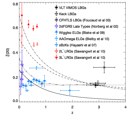
Figure 25: The volume-averaged correlation function, $\overset{\_}{\xi}(20)$, is plotted for our LBG sample alongside $\overset{\_}{\xi}(20)$ measurements for several other galaxy populations, including LRGs at $z<1$ (Sawangwit et al., 2009), star-forming galaxies at $z<1$ (Norberg et al., 2002; Bielby et al., 2010; Blake et al., 2010) and $z\sim 2$ and other LBG populations (Adelberger et al., 2003; Foucaud et al., 2003). Further to the observational data, the solid line shows the estimated evolution of the underlying dark-matter clustering using the CAMB software (Lewis et al., 2000), whilst the horizontal dotted line, dashed line and dot-dash line show the clustering evolution given no evolution in comoving coordinates, the long-lived model and the stable model. The dot-dot-dot-dash line shows the clustering evolution based on the modeling of the merger history of dark matter haloes.

5 Conclusions

In this paper we have described the VLT VIMOS survey of $z\approx 3$ galaxies in a number of fields around bright $z>3$ QSOs. In total this survey has so far produced a total of 1020 LBGs at redshifts of $2<z<3.5$ over a total area of $1.18{\rm deg}^{2}$. This concludes the data acquisition for the initial phase of the VLT VIMOS LBG Survey. At the time of writing, these are the most up to date observations, however the survey has a number of observations only recently acquired, comprising another 25 VIMOS pointings. Upon completion, the survey will comprise a total of 45 VIMOS pointings, building significantly on this initial data-set and providing a catalogue of $\approx 2,000$ $z>2$ galaxies over a sky area of $2.11\textrm{deg}^{2}$. The wide angular coverage of VLT VIMOS makes the new LBG study very complementary to the previous Keck study which has higher space densities over smaller areas and hence increased power at the smallest LBG separations but little information in the angular direction beyond $10~{}h^{-1}{\rm Mpc}$. We therefore have frequently used the two surveys in combination in the studies of LBG clustering we have presented here.

Based on the fraction of objects observed for this initial VLT LBG survey, we find that our estimated number densities are consistent with previous studies of LBGs in this redshift range. Overall we obtain a mean redshift of $\overset{\_}{z}=2.85\pm 0.34$. From the data obtained we have shown evidence for the existence of galactic outflows with comparable offsets between emission and absorption lines as in previous studies (e.g. Pettini et al. 2000, 2002 and Shapley et al. 2003)

We have further measured the clustering properties of the VLT VIMOS LBG sample. Based on the angular auto-correlation function of the photometric LBG candidates, the real-space LBG correlation function, $\xi(r)$, is estimated to take the form of a double power-law, with a break at $r_{b}\approx 1.5~{}h^{-1}{\rm Mpc}$. This is parametrised by a clustering length and slope below the break of $r_{0,1}=3.19\pm 0.55~{}h^{-1}{\rm Mpc}$, $\gamma_{1}=2.45\pm 0.15$ and above the break of $r_{0,2}=4.37^{+0.43}_{-0.55}~{}h^{-1}{\rm Mpc}$, $\gamma_{2}=1.61\pm 0.15$.

Assuming $\gamma=1.8$, the semi-projected LBG correlation function $w_{p}(\sigma)$ gives $r_{0}=3.67^{+0.23}_{-0.24}~{}h^{-1}{\rm Mpc}$ for the VLT LBGs, slightly lower than $r_{0}=4.2^{+0.14}_{-0.15}~{}h^{-1}{\rm Mpc}$ for the Keck LBGs, and the combined VLT$+$Keck sample gives $r_{0}=3.98^{+0.13}_{-0.12}~{}h^{-1}{\rm Mpc}$. At $r_{b}>1~{}h^{-1}{\rm Mpc}$, the $\xi(r)$ estimates from $w(\theta)$ and $w_{p}(\sigma)$ are therefore quite consistent. At $r_{b}<1~{}h^{-1}{\rm Mpc}$ the steeper power-law from the angular correlation function rises above the single power-law that best fits $w_{p}$, but the difference is only marginally statistically significant. These measurements of LBG clustering are broadly consistent with previous measurements of the clustering of LBGs at $z\approx 3$ made by Adelberger et al. (2003) and da Ângela et al. (2005a) but lower than those made by Foucaud et al. (2003)

We then measured the redshift-space LBG auto-correlation function, $\xi(s)$. As expected, this presents a flatter slope at scales $s<8~{}h^{-1}{\rm Mpc}$ due to the effect of velocity errors, outflows and intrinsic velocity dispersions. Both the VLT and Keck samples require total pairwise velocity dispersions in the range $<w_{z}^{2}>^{1/2}=600-1000~{}{\rm kms}^{-1}$ to fit $\xi(s)$, higher than the $<w_{z}^{2}>^{1/2}=400~{}{\rm kms}^{-1}$ previously assumed (da Ângela et al., 2005a). The VLT and Keck samples’ $\xi(s)$ results both imply an intrinsic pairwise velocity dispersion of $\pm 400~{}{\rm kms}^{-1}$ for a $\xi(r)$ model with $r_{0}=3.98~{}h^{-1}{\rm Mpc}$ and $\gamma=1.8$. A higher $<w_{z}^{2}>^{1/2}$ will imply a higher infall parameter, $\beta(z=3)$, due to the degeneracy between these parameters. The high value of the velocity dispersion will also have an impact on our search for the effects of star-formation feedback on the QSO Lyman-$\alpha$ forest (Crighton et al., 2010) because any sharp decrease in absorption near an LBG will tend to be smoothed away by this dispersion acting as an effective redshift error.

We combine our LBG sample with that of Steidel et al. (2003) with the aim of measuring the infall parameter, $\beta(z=3)$. Using a single power-law with $r_{0}=3.98~{}h^{-1}{\rm Mpc}$ and $\gamma=1.8$ as our model for the real space $\xi(r)$, our fits to our measurement of the LBG $\xi(\sigma,\pi)$ from the combined data-set produce a best fitting infall parameter of $\beta=0.48\pm 0.17$. We find that this value is consistent with the $\beta=0.37$ value expected in the standard $\Lambda$CDM cosmology. For this cosmology the value of the LBG bias implied from the galaxy dynamics is $b=2.06^{+1.12}_{-0.53}$, again consistent with the value of $b=2.22\pm 0.16$ measured from the amplitude of the LBG $\xi(r)$, assuming the standard cosmology.

We have also made the cosmological test suggested by Hoyle et al. (2002) and da Ângela et al. (2005a) and shown that the values of $\Omega_{m}^{0}$ and $\beta(z=3)$ derived from LBG redshift-space distortion are consistent with those derived by comparing the amplitude of LBG clustering at $z=3$ from the combination of the measured 2dFGRS clustering amplitude and $\beta$ at $z=0.1$, using linear theory. Our measurement of $\beta(z=3)$ is therefore consistent with what is expected from the gravitational growth rate predicted by Einstein gravity in the standard cosmological model (see Guzzo et al. 2008).

Finally, we have used the clustering amplitude measured for the LBGs to test simple models of clustering evolution. In particular, we find that if the LBGs are long-lived then they could be the progenitors of low redshift $L^{*}$ spirals or early-type galaxies by the present day.

The VLT LBG Survey is an ongoing project and we hope to double the survey area and LBG numbers by completion of the project. In combination with this work we are performing a survey of $z\approx 3$ QSOs in our LBG survey fields using the AAOmega instrument at the AAT. Bringing these two data-sets together will present a significant data resource for the study of the relationship between galaxies and the IGM at $z\approx 3$.

References

- Abazajian et al. (2005) Abazajian K., Zheng Z., Zehavi I., Weinberg D. H., Frieman J. A., Berlind A. A., Blanton M. R., Bahcall N. A., Brinkmann J., Schneider D. P., Tegmark M., 2005, ApJ, 625, 613
- Adelberger et al. (2005a) Adelberger K. L., Shapley A. E., Steidel C. C., Pettini M., Erb D. K., Reddy N. A., 2005a, ApJ, 629, 636
- Adelberger et al. (2005b) Adelberger K. L., Steidel C. C., Pettini M., Shapley A. E., Reddy N. A., Erb D. K., 2005b, ApJ, 619, 697
- Adelberger et al. (2003) Adelberger K. L., Steidel C. C., Shapley A. E., Pettini M., 2003, ApJ, 584, 45
- Aguirre et al. (2004) Aguirre A., Schaye J., Kim T.-S., Theuns T., Rauch M., Sargent W. L. W., 2004, ApJ, 602, 38
- Alcock & Paczynski (1979) Alcock C., Paczynski B., 1979, Nat, 281, 358
- Aracil et al. (2004) Aracil B., Petitjean P., Pichon C., Bergeron J., 2004, Astron. & Astrophys., 419, 811
- Bertin et al. (2002) Bertin E., Mellier Y., Radovich M., Missonnier G., Didelon P., Morin B., 2002, in Astronomical Society of the Pacific Conference Series, Vol. 281, Astronomical Data Analysis Software and Systems XI, Bohlender D. A., Durand D., Handley T. H., eds., pp. 228–+
- Bielby et al. (2010) Bielby R., Shanks T., Sawangwit U., Croom S. M., Ross N. P., Wake D. A., 2010, MNRAS, 403, 1261
- Blake et al. (2010) Blake C., Brough S., Colless M., Couch W., Croom S., Davis T., Drinkwater M. J., Forster K., Glazebrook K., Jelliffe B., Jurek R. J., Li I., Madore B., Martin C., Pimbblet K., Poole G. B., Pracy M., Sharp R., Wisnioski E., Woods D., Wyder T., 2010, MNRAS, 406, 803
- Bolzonella et al. (2000) Bolzonella M., Miralles J., Pelló R., 2000, Astron. & Astrophys., 363, 476
- Bouché & Lowenthal (2004) Bouché N., Lowenthal J. D., 2004, ApJ, 609, 513
- Bregman et al. (2009) Bregman J. N., Benjamin R. A., Bonamente M., Canizares C. R., Hornschemeier A., Jenkins E., Lockman F. J., Nicastro F., Ohashi T., Paerels F., Putman M. E., Sembach K., Schulz N., Savage B., Smith R., Yamasaki N., Yao Y., Wakker B., 2009, in ArXiv Astrophysics e-prints, Vol. 2010, astro2010: The Astronomy and Astrophysics Decadal Survey, pp. 25–+
- Bruzual & Charlot (2003) Bruzual G., Charlot S., 2003, MNRAS, 344, 1000
- Cabré & Gaztañaga (2009) Cabré A., Gaztañaga E., 2009, MNRAS, 393, 1183
- Carroll et al. (1992) Carroll S. M., Press W. H., Turner E. L., 1992, ARA&A, 30, 499
- Charlot & Fall (2000) Charlot S., Fall S. M., 2000, ApJ, 539, 718
- Cole et al. (2000) Cole S., Lacey C. G., Baugh C. M., Frenk C. S., 2000, MNRAS, 319, 168
- Conroy et al. (2008) Conroy C., Shapley A. E., Tinker J. L., Santos M. R., Lemson G., 2008, ApJ, 679, 1192
- Crain et al. (2010) Crain R. A., McCarthy I. G., Frenk C. S., Theuns T., Schaye J., 2010, MNRAS, 407, 1403
- Crain et al. (2009) Crain R. A., Theuns T., Dalla Vecchia C., Eke V. R., Frenk C. S., Jenkins A., Kay S. T., Peacock J. A., Pearce F. R., Schaye J., Springel V., Thomas P. A., White S. D. M., Wiersma R. P. C., 2009, MNRAS, 399, 1773
- Crighton et al. (2010) Crighton N. H. M., Bielby R., Shanks T., Infante L., Bornancini C. G., Bouche N., Lambas D. G., Lowenthal J. D., Minniti D., Morris S. L., Padilla N., Peroux C., Petitjean P., Theuns T., Tummuangpak P., Weilbacher P. M., Wisotzki L., Worseck G., 2010, ArXiv e-prints
- Croom et al. (2005) Croom S. M., Boyle B. J., Shanks T., Smith R. J., Miller L., Outram P. J., Loaring N. S., Hoyle F., da Ângela J., 2005, MNRAS, 356, 415
- da Ângela et al. (2005a) da Ângela J., Outram P. J., Shanks T., 2005a, MNRAS, 361, 879
- da Ângela et al. (2005b) da Ângela J., Outram P. J., Shanks T., Boyle B. J., Croom S. M., Loaring N. S., Miller L., Smith R. J., 2005b, MNRAS, 360, 1040
- da Ângela et al. (2008) da Ângela J., Shanks T., Croom S. M., Weilbacher P., Brunner R. J., Couch W. J., Miller L., Myers A. D., Nichol R. C., Pimbblet K. A., de Propris R., Richards G. T., Ross N. P., Schneider D. P., Wake D., 2008, MNRAS, 383, 565
- Davis & Peebles (1983) Davis M., Peebles P. J. E., 1983, ApJ, 267, 465
- Dekel & Silk (1986) Dekel A., Silk J., 1986, ApJ, 303, 39
- Foucaud et al. (2003) Foucaud S., McCracken H. J., Le Fèvre O., Arnouts S., Brodwin M., Lilly S. J., Crampton D., Mellier Y., 2003, Astron. & Astrophys., 409, 835
- Fry (1996) Fry J. N., 1996, ApJ Lett., 461, L65+
- González & Padilla (2010) González R. E., Padilla N. D., 2010, MNRAS, 407, 1449
- Governato et al. (1998) Governato F., Baugh C. M., Frenk C. S., Cole S., Lacey C. G., Quinn T., Stadel J., 1998, Nat, 392, 359
- Governato et al. (2010) Governato F., Brook C., Mayer L., Brooks A., Rhee G., Wadsley J., Jonsson P., Willman B., Stinson G., Quinn T., Madau P., 2010, Nat, 463, 203
- Groth & Peebles (1977) Groth E. J., Peebles P. J. E., 1977, ApJ, 217, 385
- Guzzo et al. (2008) Guzzo L., Pierleoni M., Meneux B., Branchii E., Le Fèvre O., Marinoni C., Garilli B., Blaizot J., De Lucia G., Pollo A., McCracken H. J., Bottini D., Le Brun V., Maccagni D., Picat J. P., Scaramella R., Scodeggio M., Tresse L., Vettolani G., Zanichelli A., Adami C., Arnouts S., Bardelli S., Bolzonella M., Bongiorno A., Cappi A., Charlot S., Ciliegi P., Contini T., Cucciati O., de la Torre S., Dolag K., Foucaud S., Franzetti P., Gavignaud I., Ilbert O., Iovino A., Lamareille F., Marano B., Mazure A., Memeo P., Merighi R., Moscardini L., Paltani S., Pellò R., Perez-Montero E., Pozzetti L., Radovich M., Vergani D., Zamorani G., Zucca E., 2008, Nat, 451, 541
- Hamilton (1992) Hamilton A. J. S., 1992, ApJ Lett., 385, L5
- Hawkins et al. (2003) Hawkins E., Maddox S., Cole S., Lahav O., Madgwick D. S., Norberg P., Peacock J. A., Baldry I. K., Baugh C. M., Bland-Hawthorn J., Bridges T., Cannon R., Colless M., Collins C., Couch W., Dalton G., De Propris R., Driver S. P., Efstathiou G., Ellis R. S., Frenk C. S., Glazebrook K., Jackson C., Jones B., Lewis I., Lumsden S., Percival W., Peterson B. A., Sutherland W., Taylor K., 2003, MNRAS, 346, 78
- Hayashi et al. (2007) Hayashi M., Shimasaku K., Motohara K., Yoshida M., Okamura S., Kashikawa N., 2007, ApJ, 660, 72
- Heavens & Taylor (1995) Heavens A. F., Taylor A. N., 1995, MNRAS, 275, 483
- Heckman et al. (1990) Heckman T. M., Armus L., Miley G. K., 1990, ApJS, 74, 833
- Hewett et al. (1995) Hewett P. C., Foltz C. B., Chaffee F. H., 1995, AJ, 109, 1498
- Hildebrandt et al. (2007) Hildebrandt H., Pielorz J., Erben T., Schneider P., Eifler T., Simon P., Dietrich J. P., 2007, Astron. & Astrophys., 462, 865
- Hildebrandt et al. (2009) Hildebrandt H., Pielorz J., Erben T., van Waerbeke L., Simon P., Capak P., 2009, Astron. & Astrophys., 498, 725
- Hoyle et al. (2002) Hoyle F., Outram P. J., Shanks T., Croom S. M., Boyle B. J., Loaring N. S., Miller L., Smith R. J., 2002, MNRAS, 329, 336
- Hoyle et al. (2000) Hoyle F., Szapudi I., Baugh C. M., 2000, MNRAS, 317, L51
- Jackson (1972) Jackson J. C., 1972, MNRAS, 156, 1P
- Januzzi et al. (2003) Januzzi B. T., Claver J., Valdes F., 2003, The NOAO Deep Wide-Field Survey MOSAIC Reductions
- Jenkins et al. (1998) Jenkins A., Frenk C. S., Pearce F. R., Thomas P. A., Colberg J. M., White S. D. M., Couchman H. M. P., Peacock J. A., Efstathiou G., Nelson A. H., 1998, ApJ, 499, 20
- Kaiser (1987) Kaiser N., 1987, MNRAS, 227, 1
- Kim et al. (2009) Kim H., Baugh C. M., Cole S., Frenk C. S., Benson A. J., 2009, MNRAS, 400, 1527
- Kornei et al. (2010) Kornei K. A., Shapley A. E., Erb D. K., Steidel C. C., Reddy N. A., Pettini M., Bogosavljević M., 2010, ApJ, 711, 693
- Lahav et al. (1991) Lahav O., Lilje P. B., Primack J. R., Rees M. J., 1991, MNRAS, 251, 128
- Landolt (1992) Landolt A. U., 1992, AJ, 104, 340
- Landy & Szalay (1993) Landy S. D., Szalay A. S., 1993, ApJ, 412, 64
- Lehnert et al. (1999) Lehnert M. D., Heckman T. M., Weaver K. A., 1999, ApJ, 523, 575
- Lewis et al. (2000) Lewis A., Challinor A., Lasenby A., 2000, ApJ, 538, 473
- Martin (2005) Martin C. L., 2005, ApJ, 621, 227
- Martin (2006) —, 2006, ApJ, 647, 222
- McCracken et al. (2001) McCracken H. J., Le Fèvre O., Brodwin M., Foucaud S., Lilly S. J., Crampton D., Mellier Y., 2001, Astron. & Astrophys., 376, 756
- Metcalfe et al. (1996) Metcalfe N., Shanks T., Campos A., Fong R., Gardner J. P., 1996, Nat, 383, 236
- Metcalfe et al. (2001) Metcalfe N., Shanks T., Campos A., McCracken H. J., Fong R., 2001, MNRAS, 323, 795
- Mo & White (1996) Mo H. J., White S. D. M., 1996, MNRAS, 282, 347
- Norberg et al. (2002) Norberg P., Baugh C. M., Hawkins E., Maddox S., Madgwick D., Lahav O., Cole S., Frenk C. S., Baldry I., Bland-Hawthorn J., Bridges T., Cannon R., Colless M., Collins C., Couch W., Dalton G., De Propris R., Driver S. P., Efstathiou G., Ellis R. S., Glazebrook K., Jackson C., Lewis I., Lumsden S., Peacock J. A., Peterson B. A., Sutherland W., Taylor K., 2002, MNRAS, 332, 827
- O’Meara et al. (2007) O’Meara J. M., Prochaska J. X., Burles S., Prochter G., Bernstein R. A., Burgess K. M., 2007, ApJ, 656, 666
- Orsi et al. (2008) Orsi A., Lacey C. G., Baugh C. M., Infante L., 2008, MNRAS, 391, 1589
- Padilla et al. (2010) Padilla N. D., Christlein D., Gawiser E., González R. E., Guaita L., Infante L., 2010, MNRAS, 409, 184
- Peacock (1999) Peacock J. A., 1999, ”Cosmological Physics”. Cambridge University Press, UK
- Peebles (1980) Peebles P. J. E., 1980, ”The Large-Scale Structure of the Universe”. Princeton University Press
- Péroux et al. (2005) Péroux C., Dessauges-Zavadsky M., D’Odorico S., Sun Kim T., McMahon R. G., 2005, MNRAS, 363, 479
- Pettini et al. (2003) Pettini M., Madau P., Bolte M., Prochaska J. X., Ellison S. L., Fan X., 2003, ApJ, 594, 695
- Pettini et al. (2002) Pettini M., Rix S. A., Steidel C. C., Adelberger K. L., Hunt M. P., Shapley A. E., 2002, ApJ, 569, 742
- Pettini et al. (2001) Pettini M., Shapley A. E., Steidel C. C., Cuby J.-G., Dickinson M., Moorwood A. F. M., Adelberger K. L., Giavalisco M., 2001, ApJ, 554, 981
- Pettini et al. (2000) Pettini M., Steidel C. C., Adelberger K. L., Dickinson M., Giavalisco M., 2000, ApJ, 528, 96
- Phillipps et al. (1978) Phillipps S., Fong R., Fall R. S. E. S. M., MacGillivray H. T., 1978, MNRAS, 182, 673
- Pichon et al. (2003) Pichon C., Scannapieco E., Aracil B., Petitjean P., Aubert D., Bergeron J., Colombi S., 2003, ApJ Lett., 597, L97
- Ratcliffe et al. (1998) Ratcliffe A., Shanks T., Parker Q. A., Fong R., 1998, MNRAS, 296, 191
- Reddy et al. (2008) Reddy N. A., Steidel C. C., Pettini M., Adelberger K. L., Shapley A. E., Erb D. K., Dickinson M., 2008, ApJS, 175, 48
- Richards et al. (2009) Richards G. T., Myers A. D., Gray A. G., Riegel R. N., Nichol R. C., Brunner R. J., Szalay A. S., Schneider D. P., Anderson S. F., 2009, ApJS, 180, 67
- Roche et al. (1993) Roche N., Shanks T., Metcalfe N., Fong R., 1993, MNRAS, 263, 360
- Roche et al. (2002) Roche N. D., Almaini O., Dunlop J., Ivison R. J., Willott C. J., 2002, MNRAS, 337, 1282
- Ross et al. (2007) Ross N. P., da Ângela J., Shanks T., Wake D. A., Cannon R. D., Edge A. C., Nichol R. C., Outram P. J., Colless M., Couch W. J., Croom S. M., de Propris R., Drinkwater M. J., Eisenstein D. J., Loveday J., Pimbblet K. A., Roseboom I. G., Schneider D. P., Sharp R. G., Weilbacher P. M., 2007, MNRAS, 381, 573
- Sawangwit et al. (2009) Sawangwit U., Shanks T., Abdalla F. B., Cannon R. D., Croom S. M., Edge A. C., Ross N. P., Wake D. A., 2009, ArXiv e-prints
- Sawicki & Thompson (2006) Sawicki M., Thompson D., 2006, ApJ, 642, 653
- Schlegel et al. (1998) Schlegel D. J., Finkbeiner D. P., Davis M., 1998, ApJ, 500, 525
- Shapley et al. (2003) Shapley A. E., Steidel C. C., Pettini M., Adelberger K. L., 2003, ApJ, 588, 65
- Sheth et al. (2001) Sheth R. K., Mo H. J., Tormen G., 2001, MNRAS, 323, 1
- Smith et al. (2003) Smith R. E., Peacock J. A., Jenkins A., White S. D. M., Frenk C. S., Pearce F. R., Thomas P. A., Efstathiou G., Couchman H. M. P., 2003, MNRAS, 341, 1311
- Songaila & Cowie (1996) Songaila A., Cowie L. L., 1996, AJ, 112, 335
- Springel et al. (2006) Springel V., Frenk C. S., White S. D. M., 2006, Nat, 440, 1137
- Springel et al. (2005) Springel V., White S. D. M., Jenkins A., Frenk C. S., Yoshida N., Gao L., Navarro J., Thacker R., Croton D., Helly J., Peacock J. A., Cole S., Thomas P., Couchman H., Evrard A., Colberg J., Pearce F., 2005, Nat, 435, 629
- Steidel et al. (2003) Steidel C. C., Adelberger K. L., Shapley A. E., Pettini M., Dickinson M., Giavalisco M., 2003, ApJ, 592, 728
- Steidel et al. (2010) Steidel C. C., Erb D. K., Shapley A. E., Pettini M., Reddy N., Bogosavljević M., Rudie G. C., Rakic O., 2010, ApJ, 717, 289
- Steidel et al. (1996) Steidel C. C., Giavalisco M., Pettini M., Dickinson M., Adelberger K. L., 1996, ApJ Lett., 462, L17+
- Steidel & Hamilton (1993) Steidel C. C., Hamilton D., 1993, AJ, 105, 2017
- Steidel et al. (2004) Steidel C. C., Shapley A. E., Pettini M., Adelberger K. L., Erb D. K., Reddy N. A., Hunt M. P., 2004, ApJ, 604, 534
- Steinmetz & Navarro (1999) Steinmetz M., Navarro J. F., 1999, ApJ, 513, 555
- Tummuangpak et al. (In prep) Tummuangpak N., Shanks T., Crighton N. H. M., Bielby R., In prep, MNRAS
- Wake et al. (2008) Wake D. A., Sheth R. K., Nichol R. C., Baugh C. M., Bland-Hawthorn J., Colless M., Couch W. J., Croom S. M., de Propris R., Drinkwater M. J., Edge A. C., Loveday J., Lam T. Y., Pimbblet K. A., Roseboom I. G., Ross N. P., Schneider D. P., Shanks T., Sharp R. G., 2008, MNRAS, 387, 1045
- White & Frenk (1991) White S. D. M., Frenk C. S., 1991, ApJ, 379, 52
- Wiersma et al. (2009) Wiersma R. P. C., Schaye J., Theuns T., Dalla Vecchia C., Tornatore L., 2009, MNRAS, 399, 574
- Williger et al. (1996) Williger G. M., Hazard C., Baldwin J. A., McMahon R. G., 1996, ApJS, 104, 145
- Wilman et al. (2005) Wilman R. J., Gerssen J., Bower R. G., Morris S. L., Bacon R., de Zeeuw P. T., Davies R. L., 2005, Nat, 436, 227
- Yoshida et al. (2008) Yoshida M., Shimasaku K., Ouchi M., Sekiguchi K., Furusawa H., Okamura S., 2008, ApJ, 679, 269
- Zheng et al. (2005) Zheng Z., Berlind A. A., Weinberg D. H., Benson A. J., Baugh C. M., Cole S., Davé R., Frenk C. S., Katz N., Lacey C. G., 2005, ApJ, 633, 791
- Zheng et al. (2009) Zheng Z., Zehavi I., Eisenstein D. J., Weinberg D. H., Jing Y. P., 2009, ApJ, 707, 554