Cluster Galaxy Dynamics and the Effects of Large Scale Environment

Abstract

Advances in observational capabilities have ushered in a new era of multi-wavelength, multi-physics probes of galaxy clusters and ambitious surveys are compiling large samples of cluster candidates selected in different ways. We use a high-resolution N-body simulation to study how the influence of large-scale structure in and around clusters causes correlated signals in different physical probes and discuss some implications this has for multi-physics probes of clusters (e.g. richness, lensing, Compton distortion and velocity dispersion).

We pay particular attention to velocity dispersions, matching galaxies to subhalos which are explicitly tracked in the simulation. We find that not only do halos persist as subhalos when they fall into a larger host, groups of subhalos retain their identity for long periods within larger host halos. The highly anisotropic nature of infall into massive clusters, and their triaxiality, translates into an anisotropic velocity ellipsoid: line-of-sight galaxy velocity dispersions for any individual halo show large variance depending on viewing angle. The orientation of the velocity ellipsoid is correlated with the large-scale structure, and thus velocity outliers correlate with outliers caused by projection in other probes. We quantify this orientation uncertainty and give illustrative examples. Such a large variance suggests that velocity dispersion estimators will work better in an ensemble sense than for any individual cluster, which may inform strategies for obtaining redshifts of cluster members. We similarly find that the ability of substructure indicators to find kinematic substructures is highly viewing angle dependent. While groups of subhalos which merge with a larger host halo can retain their identity for many Gyr, they are only sporadically picked up by substructure indicators.

We discuss the effects of correlated scatter on scaling relations estimated through stacking, both analytically and in the simulations, showing that the strong correlation of measures with mass and the large scatter in mass at fixed observable mitigate line-of-sight projections.

1 Introduction

Galaxy clusters form the high-mass tail of hierarchical structure formation and are of interest for constraining cosmological parameters, understanding large scale structure, as extreme environments for galaxy formation and as objects hosting unique astrophysical phenomena. While first discovered as concentrations of galaxies (Abell, 1958; Zwicky et al., 1966), they are now also routinely found as luminous, extended X-ray sources (Schwartz, 1978; McHardy, 1978; Bohringer et al., 2000, 2001), as peaks in the shear field (Wittman et al., 2006) and as “holes” in the microwave sky (Staniszewski et al., 2009). To mitigate the systematic errors associated with each individual method and to provide a more complete understanding of clusters, multi-wavelength studies have become increasingly common. Each waveband adds knowledge about clusters. However, we might expect there to be significant correlations between effects in different methods both because the intrinsic properties they measure depend on e.g. cluster size but also because they are similarly affected by the complex environment surrounding clusters.

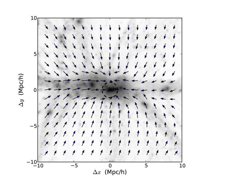
Figure 1: The velocity field traces the filamentary large-scale structure. The grey scale shows the logarithm of the projected dark matter density in a $5\,h^{-1}$Mpc thick slice around a cluster of mass $5\times 10^{14}\,h^{-1}M_{\odot}$ at $z=0$. The slice is oriented to contain the halo particle velocity eigenvectors with the largest ($x$) and smallest ($y$) eigenvalues. The dashed circle shows the region within $r_{200c}$. Note that within the cluster the velocities trace the elongation of the matter, as required. In addition the velocities at larger distances trace the filamentary structure in the larger scale environment. Thus we expect that velocity anisotropy will be correlated with density anisotropy.

Roughly speaking, both the hot gas and galaxies in clusters trace the dark matter which dominates the potential. We can approximate the clusters as self-similar and isothermal, with a temperature $T\propto M^{2/3}$, a velocity dispersion $\sigma^{2}\propto T$, and richness $N\propto M$ for sufficiently massive halos (Kaiser, 1986). Consider a small region near the cluster: lensing measures the sum of all of the mass, richness all of the mass in halos above some threshold and Compton (or SZ) distortion (Sunyaev & Zel’dovich, 1972, SZ) all of the mass in halos weighted by $M^{2/3}$. The signal in each probe depends on the mass within the virialized region of the cluster, the mass near the cluster but outside the virial region and (uncorrelated) mass at larger distance along the line-of-sight. Lensing and Compton distortion measures provide little line-of-sight resolution. The degree of projection involved in a richness estimator depends on how well the galaxy distances are known (e.g. using photometric or spectroscopic redshifts).

Line-of-sight galaxy velocities in principle provide a measure of the potential well depth or mass and offer the possibility of breaking line-of-sight projection. However, the velocity field traces the density field, and can be correlated with line-of-sight projection due to the filamentary nature of mass accretion onto massive halos (see Fig. 1 which gives an example of this effect in our simulations). The velocities of cluster galaxies can retain this large scale anisotropy (see also Tormen, 1997; Kasun & Evrard, 2005, for studies of dark matter velocities). Thus it is easy to imagine that line-of-sight velocity dispersion could be correlated with filamentary material which can bias individual cluster measurements in e.g. richness, lensing or Compton distortion.

We would like to investigate how the complex structure of the cosmic web of material near clusters leads to correlations in individual cluster observables, and the implications that this has for these four probes of clusters. This shared dependence, not only on cluster properties but also on cluster environment, can introduce additional subtleties when methods are combined. For example, an often used approach is to “stack” clusters on the basis of one observed property $X$ (e.g. richness), and then look for correlations between two other properties, $Y$ and $Z$. Clearly, it is very important to understand the joint distribution $P(X,Y,Z)$ and the degree of correlation between scatter in $X$, $Y$ or $Z$.

In this paper we use N-body numerical simulations with subhalos (which we identify with galaxies) to study properties of cluster galaxy kinematics and the relation of the scatters in velocity dispersion, Compton distortion, lensing, and optical richness generated by nearby large-scale structure. Details of our numerical simulations and methods for finding subhalos are given in §2. We describe how the mock richness, lensing and Compton distortion observations are constructed in §3. Readers interested in the results may skip to §4 where we discuss the intrinsic properties of our massive halos and their subhalo (galaxy) populations and §5 where we discuss measurements of galaxy kinematics in the presence of interlopers and §6 where we discuss the correlations between different observables.

The effects of the cosmic web, and in particular projection effects, have been long-time concerns for optical cluster finding (e.g. Abell, 1958; Dalton et al, 1992; Lumsden et al, 1992; van Haarlem et al., 1997; White et al, 1999), measuring Compton distortion (e.g. White, Hernquist & Springel, 2002; Holder, McCarthy & Babul, 2007; Hallman et al, 2007; Shaw, Holder & Bode, 2008), or interpreting weak lensing maps (e.g. Reblinsky & Bartelmann, 1999; Metzler, White & Loken, 2001; Hoekstra, 2001; de Putter & White, 2005; Meneghetti et al., 2010). Correlations between scatters induced by common projection effects were noted in Cohn & White (2009). Cen (1997) did an early simulation study of projection on several of the indicators we consider here including richness, velocity dispersions and lensing, and measured substructure using dark matter particles. For cluster kinematics in particular, the velocity dispersion properties of dark matter particles and their relation to the cosmic web were studied in Tormen (1997); Kasun & Evrard (2005) and Biviano et al. (2006) noted that filamentary inflow was expected to affect measured velocity dispersions. Our simulations have enough dynamic range that we can simulate a representative cosmological volume, including the neighboring large-scale structure and cosmic web, while simultaneously resolving and tracking the subhalos which we believe are galactic hosts. This preserves any correlations between subhalo properties and halo orientation or cosmic web, and coherence between subhalo populations which fell in as part of a group. We emphasize the effect that anisotropy in galaxy kinematics has on line-of-sight velocity dispersion or virial mass estimators of cluster mass and discuss how this scatter compares to (and correlates with) other measures of cluster mass which are sensitive to the cluster’s environment. This forms a partial extension of the work of Stanek et al. (2010), who discussed the correlations in scatters of a large number of different intrinsic (rather than projected) cluster quantities, including X-ray.

2 Simulations

In order to investigate the above questions with ‘realistic’ conditions we need mock galaxy, gas and lensing catalogs in which clusters of galaxies are placed in their correct cosmological context, with an appropriate prescription for identifying galaxies and for which the intrinsic cluster properties are known. We make use of several dark-matter-only N-body simulations. Such simulations follow the evolution of large dark matter halos, which we observe as galaxy clusters, correctly accounting for their place in the filamentary large-scale structure and their complex formation histories.

2.1 N-body simulation

We make use of several simulations in this paper. The main one is of the $\Lambda$CDM family with $\Omega_{m}=0.274$, $\Omega_{\Lambda}=0.726$, $h=0.7$, $n=0.95$ and $\sigma_{8}=0.8$, in agreement with a wide array of observations. Briefly, we used the TreePM code described in White (2002) to evolve $2048^{3}$ equal mass particles in a periodic cube of side length $250\,h^{-1}$Mpc. This results in particle masses of $1.4\times 10^{8}\,h^{-1}M_{\odot}$ and a Plummer equivalent smoothing of $2.5\,h^{-1}$kpc. The initial conditions were generated by displacing particles from a regular grid using second order Lagrangian perturbation theory at $z=150$ where the rms displacement is $38$ per cent of the mean inter-particle spacing. The phase space data were dumped at 45 times, equally spaced in $\ln(a)$ from $z=10$ to $0$. This TreePM code has been compared to a number of other codes and shown to perform well for such simulations (Heitmann et al., 2008). Though we shall not highlight them individually, in addition to this simulation we have made use of the simulation described in Wetzel & White (2010), which used a different subhalo finder, and four other simulations of smaller volumes focused on massive halos where we have mass resolution $2-5$ times higher than in the fiducial run and comparably higher force resolution. This allows us to check the dependence on subhalo finding and tracking scheme, mass and force resolution and on limiting mass.

For each output we found dark matter halos using the Friends of Friends (FoF) algorithm (Davis et al., 1985) with a linking length of $0.168$ times the mean interparticle spacing. This partitions the particles into equivalence classes roughly bounded by isodensity contours of $100\times$ the mean density. We keep all halos above $50$ particles, and generate merger trees for all of the halos in the simulation so as to identify the times of last major mergers or other interesting events in the history. The center of the halo is taken to be the position of the most bound particle, including all of the mass in the Friends of Friends halo in the computation of the potential.

Given halo centers, we also compute the spherically averaged mass profile taking into account all of the mass in the simulation. We follow standard convention and define the virial radius as that radius within which the mean density is $200$ times the critical density at the epoch of observation, writing this $r_{200c}$. The three dimensional velocity dispersion of the dark matter within $r_{200c}$ is tightly correlated with the mass interior to the same radius as expected from the virial relation (e.g. Evrard et al., 2008, for a recent study). The mass function of halos is approximately universal if a density contrast tied to the mean density and encompassing the zero-velocity surface is used (Jenkins et al., 2001; White, 2001; Robertson et al., 2009; Bhattacharya et al., 2010). When appropriate we also use the radius within which the mean density is $180$ times the background density, $r_{180b}$, for convenience. Unless stated below, the mass quoted will be $M_{180b}$.

2.2 Subhalos/Galaxies

In hierarchical structure formation models, such as CDM, the virialized regions of large dark matter halos contain subhalos — self-gravitating, bound clumps of dark matter — which contain $\mathcal{O}(10)$ per cent of the total halo mass. Luminous galaxies form via the cooling and condensation of baryons in the very centers of halos and subhalos so these subhalos identify the sites of galaxy formation in the simulation.

We identify “subhalos” within our Friends of Friends halos as overdensities in phase space (see Appendix A). For newly formed halos the “central” subhalo is defined as the most massive subhalo within the host. For other halos it is defined as the descendant of the central subhalo within the most massive progenitor of the host halo. The subhalo position is that of its most bound particle. Subhalo merger trees are computed as described in Wetzel, Cohn & White (2009) and Wetzel & White (2010). Briefly, subhalo histories are tracked across 4 consecutive output times to ensure subhalos are not “lost” during close passes through the dense central regions of a halo. Parent-child relationships are determined using the 20 most bound particles (which we have found to be very stable). For each subhalo we define $M_{\rm inf}$ as the host halo mass it had just prior to becoming a satellite, i.e. the largest host halo mass for which it was the central subhalo. We shall use $M_{\rm inf}$ as a proxy for stellar mass or luminosity and keep all subhalos whose infall mass is larger than $2\times 10^{11}\,h^{-1}M_{\odot}$ ($>10^{3}$ particles). Resolution tests indicate the catalogs are largely complete to this mass limit (see also Boylan-Kolchin et al. 2009).

As discussed extensively in Wetzel & White (2010) there are slightly more satellites per host halo, and correspondingly more small-scale clustering power, than observations demand. If we remove the excess based on the ratio of instantaneous subhalo mass to infall mass (Wetzel & White, 2010) and match subhalos to galaxies based on abundance then our halo catalog is in good agreement with many observations including the global and cluster luminosity functions, the satellite statistics and the luminosity dependent clustering of galaxies.

We shall focus primarily on $z\simeq 0.1$, discussing what changes as we go to higher redshift in §7. At $z=0.1$, the number density of subhalos above our mass threshold is $0.02h^{-3}{\rm Mpc}^{3}$. Observationally the same number densities are achieved by going down to $0.2\,L_{\star}$ or $M_{r}=-18.5$ in the r-band (Blanton et al., 2003) or about $M_{B}=-18.6$ (Faber et al., 2007) or a stellar mass of about $3\times 10^{9}\,h^{-1}M_{\odot}$ (Moster et al., 2010).

As our simulation explicitly tracks the evolution of subhalos, including their complex dynamics and mass loss, we are in a position to ask sophisticated questions about the spatial and kinematic distribution of “galaxies” in clusters. As shown below, the subhalo spatial distribution and its environment dependence is in good agreement with corresponding observations of galaxies. By using subhalos, rather than just randomly drawing particles from within the halo, we ensure that we keep any correlations between subhalo positions and the halo orientation or its large-scale environment (see e.g. Faltenbacher et al., 2009; Siverd, Ryden & Gaudi, 2010, for recent reviews) and between positions and dynamics of subhalos that fell into the host as part of a larger group.

Figure 2: The halo occupation distribution for our clusters at $z\sim 0.1$ (points), compared to the SDSS group catalogs of Yang, Mo & van den Bosch (2008, solid lines) for two different luminosity thresholds. Subhalo masses are converted to $r$-band luminosity by abundance matching, assuming a 1-1 relation (i.e. no scatter). The panels correspond to lg$M>11.7$ and 12.2 respectively, with masses measured in $h^{-1}M_{\odot}$. For each cluster the halo mass is defined as that interior to $r_{180b}$, within which the mean matter density is 180 times the background density. The richness is defined as all galaxies above a phase-space density threshold, as in the observations. We plot 30 lines-of-sight per halo.

Figure 3: The (projected) subhalo profile for galaxies brighter than $0.4\,L_{\star}$ (i.e. $M_{\star}+1$), normalized at the virial radius. The curves show a simple singular isothermal sphere ($\Sigma\propto R^{-1}$) and the profile Lin, Mohr & Stanford (2004) found which fits the counts of $K$-band selected galaxies at $z\simeq 0.1$.

Figure 4: The isotropically averaged 1D velocity dispersion of the dark matter vs. the satellite subhalos for halos with more than 50 members at $z\simeq 0.1$. The points are for all particles and satellites within spheres of radius $r_{200c}$ (crosses) and $r_{100c}$ (squares) about the most bound particle in the halo. The short-dashed line represents equality and the dotted ($r_{200c}$) and long-dashed ($r_{100c})$ lines are an unweighted fit to the points.

In Figure 2 we demonstrate that the halo occupation distribution of galaxies in the simulation is in good agreement with the measurements from the group catalog in Yang, Mo & van den Bosch (2008). Our satellite spatial distribution is slightly shallower than the dark matter in the central regions. The (projected) profile matches well the NFW profile found to fit the counts of $K$-band selected galaxies by Lin, Mohr & Stanford (2004) down to $r\simeq 0.1\,r_{200c}$, see Figure 3.

We find evidence for mild positive velocity bias within the virial sphere (Fig. 4), in agreement with most previous work (Gao et al., 2004; Goto, 2005; Faltenbacher & Diemand, 2006; Lau, Nagai & Kravtsov, 2010; Faltenbacher, 2010). The velocities of satellites appears to be determined almost entirely by the hosts’ potential (Wetzel, 2010), although we caution that the degree of velocity bias does depend on the manner in which subhalos are selected and retained, with more massive satellites showing reduced dispersion and satellites accreted more recently generally having increased dispersion. This may become important as we move to higher redshift where the mean mass of the host halos should decrease while the mean mass of the halos for which one could obtain accurate redshifts should increase, leading to a smaller mass ratio and larger effects of dynamical friction. This is partially canceled by the “more recent” infall time distribution at higher redshift. In summary, the exact amount of velocity bias will depend on how the subhalo samples are selected (Gao et al., 2004; Goto, 2005; Faltenbacher & Diemand, 2006; Lau, Nagai & Kravtsov, 2010; Faltenbacher, 2010), and can evolve with redshift – since it is not entirely clear how to match an observed galaxy sample to a particular subhalo sample it seems prudent to assign a $\mathcal{O}(10)$ per cent theoretical uncertainty in the absolute value of the velocity bias with a roughly comparable scatter from halo to halo.

2.3 Missing physics

Our simulations do not attempt to model the baryonic component, and thus can only be an approximation to the full story. Fortunately for the most massive objects in the universe, the majority of the baryonic material is in hot gas, rather than cold gas or stars. The cooling of gas in massive clusters does not dramatically alter the halo profile, except in the very inner regions (e.g. Kazantzidis et al, 2004) Outside of these regions the spatial distribution of the hot gas largely follows the gravitational potential and we shall make this assumption where necessary. The hot intra-cluster medium in massive halos is expected to alter the orbits of satellites only mildly (Simha et al, 2009; Lau, Nagai & Kravtsov, 2010; Jiang, Jing & Lin, 2010), since it is a minority mass component and they are traveling at close to the sound speed (e.g. Conroy & Ostriker, 2008). The cooling of gas in the centers of our subhalos could help to stabilize them against disruption. Our numerical resolution is high enough that the relevant subhalos are not lost to numerical disruption in any case, and our satellite fractions are at or above observational estimates (see Wetzel & White, 2010, for a compilation). The outer envelope which is lost to stripping is expected to be mostly dark matter, so this physics will be correctly modeled. Once a majority of the mass is lost the subhalo mass will be much less than the host halo mass, and the amount of dynamical friction experienced will be small, mitigating any error in the precise amount (Simha et al, 2009; Lau, Nagai & Kravtsov, 2010; Jiang, Jing & Lin, 2010). Extending high dynamic range simulations such as ours with additional physics which is in accord with observational constraints would be very interesting.

3 Mock observations

Given the matter and subhalo distribution, we compute a number of mock observations to investigate how the complicated nature of structure formation influences observational probes of clusters. In all cases we use constant time outputs from the simulation, and consider the box in isolation, i.e. we do not attempt to make light cones, remap or stack boxes. Our simulations contain sufficient path length to answer the questions of interest to us here without needing to employ these techniques. Also, we do not model the cluster finding process itself. Rather we ask about the measurements that could be made once a cluster was correctly identified.

To identify correlations due to the anisotropic nature of the cluster and its environment, we observe each cluster along 96 different lines of sight, centering it within the periodic box. (For intrinsic measurements in §4 more sightlines are considered, when needed, as described therein.) Each line of sight then is used to find galaxy richness, velocity dispersion, lensing and integrated Compton distortion. Our resulting sample has 83 clusters with $M_{180b}\geq 2\times 10^{14}\,h^{-1}M_{\odot}$ along almost $8,000$ lines of sight total, and 242 clusters with $M_{180b}\geq 10^{14}\,h^{-1}M_{\odot}$ along $\sim 23,000$ lines of sight.

3.1 Richness

The easiest property of a cluster to observe is its “richness”, or the number of galaxies it contains. Each halo above any infall mass threshold, $M_{\rm min}$, hosts one central subhalo above the same threshold mass, and a number of satellite subhalos which is (approximately) Poisson distributed about a mean $(M_{\rm halo}/M_{1})$ with $M_{1}\sim 15\,M_{\rm min}$. Unfortunately this information is not observationally accessible, and proxies must be used. There are numerous definitions of richness in the literature, here we consider only two as representative of the class.

The first is the richness defined by Yang, Mo & van den Bosch (2008), which computes a phase space density for each cluster and assigns galaxies above a threshold to a cluster candidate. The richness is the number of galaxies assigned. Rather than iterate our fit, we use the cluster’s true mass in the model, but otherwise implement the method as they describe, including all galaxies within the simulation, not just true cluster members, in the calculation. As shown in Fig. 2 the richness measured in our simulations is in quite good agreement with that inferred from the observations and the richness does show strong trends with host halo mass. However it does require knowledge of the spectroscopic redshifts of all galaxies. We call this quantity phase space richness below.

A second richness definition counts only those galaxies within the red sequence and within an aperture, subtracting an estimate of the contamination. The hope is that using only these galaxies reduces the impact of interloper galaxies from large line-of-sight distance and blue galaxies in front of the cluster, without requiring spectroscopic redshift information(see, e.g. Gladders & Yee, 2000, 2005). This requires us to assign a color to each of our mock galaxies. By abundance matching we are able to assign a luminosity (or stellar mass) to all of our subhalos. We use the method of Skibba & Sheth (2009) to further assign them a color and we include them in the projected red sequence based upon their distance from the true cluster redshift (this method has only been calibrated at $z\simeq 0.1$ so we do not assign colors when considering higher $z$). Further details are given in Appendix B. The richness includes galaxies brighter than $0.4\,L_{\star}$ (i.e. $M_{\star}+1$) with the background subtraction computed precisely using the periodic simulation volume. The transverse aperture is set following the convention used in the maxBCG catalog (Koester et al. 2007; see also High et al 2010): a first estimate of the richness is obtained within a $1\,h^{-1}$Mpc transverse radius and this richness is used to estimate $R_{200b}$ which is then used for a final richness estimate. Our final richness-mass relation (not shown) is in good agreement with the scaling relation found in observed clusters. Note that this procedure has the unwelcome property of increasing scatter due to filament-based projection effects. Should the initial estimate be high due to projected galaxies the aperture will be set too large and include even more galaxies. We noted a large increase in richness scatter at fixed mass using this procedure relative to when we use the true radii.

3.2 Galaxy kinematics

Modeling of galaxy kinematics in clusters remains a major tool in determining their properties. Since we are able to resolve and track the subhalos which would host galaxies within our simulation, we are in a good position to study how their velocity structure depends upon and correlates with cluster properties and the larger environment. As this capability is new in terms of mock velocity observations, we shall develop it in some detail in the next two sections. The intrinsic properties of the velocity field, including velocity bias, were discussed in §2.2. Anisotropy and substructure are discussed in §4. Our modeling of interloper rejection and dispersion estimation is the subject of §5.

3.3 Lensing

The distribution of mass can be probed by the distortion of background galaxy shapes due to the gravitational deflection of light by the potentials of massive halos. This signal is sensitive to the projected mass along the line-of-sight, $\Sigma$, weighted by a kernel (e.g. Hoekstra, Yee & Gladders, 2002; Refregier, 2003, for recent reviews). The lensing kernel varies only very slowly with distance, so all of the matter in and around the cluster receives similar weight. If we assume the source and lens redshift (distributions) are known, lensing measures the projected mass. We do not attempt to model the full light cone here, rather we make the approximation that mass far from the cluster is uncorrelated with the cluster and contributes only a “noise” while mass close to the cluster receives the same weight as the cluster itself. We ignore the noise term (and any additional noise from the finite number of source galaxies or observational non-idealities) and approximate a lensing observation as a measurement of the projected mass, apodized with a Welch kernel

$$W(z)=1-\left(\frac{2Z}{L_{\rm box}}\right)^{2}$$ (1)

where $-\frac{1}{2}L_{\rm box}<Z<\frac{1}{2}L_{\rm box}$ is the line-of-sight coordinate. The window vanishes for $|Z|>\frac{1}{2}L_{\rm box}$. We model all lensing observations as applying to $\Sigma(R)$ determined in this manner along any line-of-sight, using the periodicity of the box to place the lensed object at the center of the box.

A detailed study of lensing projection effects is not the focus of this paper. It has been discussed in detail previously (Reblinsky & Bartelmann, 1999; Metzler, White & Loken, 2001; Hoekstra, 2001; de Putter & White, 2005; Meneghetti et al., 2010). In order to gauge the approximate size of the effect and its degree of correlation with other measures of cluster size we simply fit a singular-isothermal-sphere model ($\rho\propto r^{-2}$) to the lensing signal. In order to remove much of the uncorrelated signal we use the $\zeta$ statistic

$$\zeta(R_{0};R_{1},R_{2})\propto\left\langle\Sigma(R<R_{0})\right\rangle-\left\langle\Sigma(R_{1}<R<R_{2})\right\rangle$$ (2)

where the constant of proportionality depends on the source and lens redshift distributions which we shall assume known for simplicity. For our singular-isothermal-sphere this gives

$$\zeta\propto\frac{\sigma_{\rm lens}^{2}}{G}\left(\frac{1}{R_{0}}-\frac{1}{R_{1}+R_{2}}\right)$$ (3)

as a function of $R_{0}$ at fixed $R_{1}$ and $R_{2}$ which we use to fit for $\sigma_{\rm lens}$. The results are quite stable to variations in the $R_{i}$, for our fiducial results we fit $R_{0}$ in the range $0.1\,r_{180b}$ to $r_{180b}$ with $R_{1}=r_{180b}$ and $R_{2}=1.25\,r_{180b}$. Qualitatively similar results are obtained if we fit directly to the projected mass, $\Sigma(R)$, or use a different profile such as the broken power-law of Navarro, Frenk & White (1997).

3.4 Sunyaev-Zel’dovich effect

Another method for finding and weighing galaxy clusters is to study the distortion they introduce in the cosmic microwave background (CMB). The “hot” electrons in the intra-cluster medium can scatter the “cold” CMB photons to higher energy, distorting the spectrum in predictable ways (Sunyaev & Zel’dovich, 1972). The surface brightness of the Compton distortion is independent of distance, and the integrated signal is proportional to the total thermal energy of the gas, making this a powerful means for finding and characterizing clusters. The insensitivity to distance, however, means that SZ experiments must also contend with projection effects. Assuming a self-similar cluster, the Compton distortion scales as $M^{5/3}$, so lower mass halos contribute fractionally less than they do to a lensing or galaxy measure, but the relatively lower resolution of the observations exacerbates the problem.

In earlier work (Cohn & White, 2009) we investigated optical and SZ methods for finding clusters and found that the scatter from the cluster candidates in these two methods was correlated. We continue that investigation here, using a simple model of the Compton distortion appropriate to low-resolution observations (such as provided by the South Pole Telescope or Atacama Cosmology Telescope). We assign to each dark matter particle in the simulation a “mean” temperature based on the velocity dispersion of its parent halo, and compute the total Compton distortion as a sum of the mass times the temperature in cylinders, apodizing the signal as above (Eq. 1). This misses contributions to the temperature from e.g. shocks, small-scale structure in the intra-cluster gas and the run of temperature with radius. For partially resolved cluster observations however the low-order properties of the maps so obtained are in reasonable agreement with hydrodynamic simulations which include these effects (e.g. White, Hernquist & Springel, 2002), and serve to illustrate our main points. We shall use as our observable the integrated Compton $y$-parameter within a disk of radius $r_{180b}$, as this is a more stable quantity than e.g. central decrement.

4 Halo Intrinsic properties

4.1 Halos

Figure 5: The distribution of $\lambda_{2}/\lambda_{1}$ (dotted) and $\lambda_{3}/\lambda_{1}$ (dashed) for all halos more massive than $2\times 10^{14}\,h^{-1}M_{\odot}$ at $z=0.1$. Thick lines show the results for subhalos within the FoF halos and thin lines for subhalos within $r_{180b}$ of the most bound particle in each group. Note that the eigenvalues, $\lambda$, of the velocity anisotropy tensor scale as $\lambda\sim\sigma^{2}$.

We begin by considering the intrinsic properties of our massive halos and their subhalo populations, absent any line-of-sight projection or misidentifications. It is well known that the 3D density profile of massive halos is triaxial (Thomas & Couchman, 1992; Warren et al, 1992; Jing & Suto, 2002), with the major axis approximately twice as long as the minor axes which are approximately equal in size. When spherically averaged the density profiles of the ‘relaxed’ halos resemble a broken power-law (Navarro, Frenk & White, 1997) with the inner regions forming early and then remaining approximately constant as subsequently accreted dark matter is kept away from the center by the angular momentum barrier. Our subhalos follow a profile similar to that of the dark matter, though shallower in the central regions.

4.2 Velocity ellipsoid

Figure 6: The distribution of $\delta\sigma_{\rm los}^{2}/\langle\sigma_{\rm los}^{2}\rangle$ for all halos more massive than $2\times 10^{14}\,h^{-1}M_{\odot}$ at $z=0$. As in Fig. 5 thick lines show the results for subhalos within the FoF halos and thin lines for subhalos within $r_{200}$ of the most bound particle in each group.

Although the 3D, dark matter velocity dispersion within $r_{200c}$ is well correlated with $M_{200c}$ (e.g. Evrard et al., 2008) and the galaxies show little velocity bias compared to the dark matter, the line-of-sight velocity dispersions show considerably more scatter. The galaxy line-of-sight dispersion for any viewing angle, $\hat{n}$, is simply $\sigma_{\rm los}^{2}=\hat{n}^{T}\cdot\sigma\cdot\hat{n}$, where $\sigma^{2}_{ij}$ is the anisotropy tensor, $\sigma^{2}_{ij}=\langle(v-\bar{v})_{i}(v-\bar{v})_{j}\rangle$, averaged over subhalos in the host halo. As has been noted before in the dark matter particles (Tormen, 1997; Kasun & Evrard, 2005), and seen here for the galaxy subhalos as well, the velocity tensor, like the moment of inertia tensor, is quite anisotropic (see also Fig. 1). Not surprisingly the principal axes of the two are quite well aligned, with a typical mis-alignment angle of $\sim 20-30^{\circ}$.

If we order the eigenvalues of $\sigma_{ij}^{2}$ as $\lambda_{1}>\lambda_{2}>\lambda_{3}$ then for uniformly chosen $\hat{n}$ the distribution of $\sigma_{\rm los}^{2}$ has a peak at $\lambda_{2}$, a mean at $\frac{1}{3}(\lambda_{1}+\lambda_{2}+\lambda_{3})$ and a width

$$\left(\delta\sigma_{\rm los}^{2}\right)^{2}=\frac{4}{45}\left[\lambda_{1}^{2}+\lambda_{2}^{2}+\lambda_{3}^{2}-\lambda_{1}\lambda_{2}-\lambda_{2}\lambda_{3}-\lambda_{3}\lambda_{1}\right]$$ (4)

For our sample, the distribution of eigenvalues for all halos above $2\times 10^{14}\,h^{-1}M_{\odot}$ at $z=0$ is shown in Fig. 5, where we see typical values for $\lambda_{3}/\lambda_{1}$ and $\lambda_{2}/\lambda_{1}$ are $0.3$ and $0.6$ respectively. For the more massive subhalos the spread in eigenvalues is slightly larger than for a random subset of the mass but they become increasingly comparable as we move down the subhalo mass function.

We found that the distribution of measured velocity dispersion for any cluster, along 10,000 randomly selected lines of sight, tended to be significantly non-Gaussian. The distribution of $\delta\sigma_{\rm los}^{2}$ from Eq. 4 is shown for our massive halos in Fig. 6, we see that $\delta\sigma_{\rm los}^{2}/\sigma_{\rm los}^{2}$ is peaked at 20-30 per cent. If one assumes $M\propto\sigma_{\rm los}^{3}$ this gives an inferred mass error of nearly 40 per cent. This suggests that, even absent any interlopers, velocity bias, or observational non-idealities, velocity dispersion mass estimators will work better in an ensemble sense than for any individual cluster.

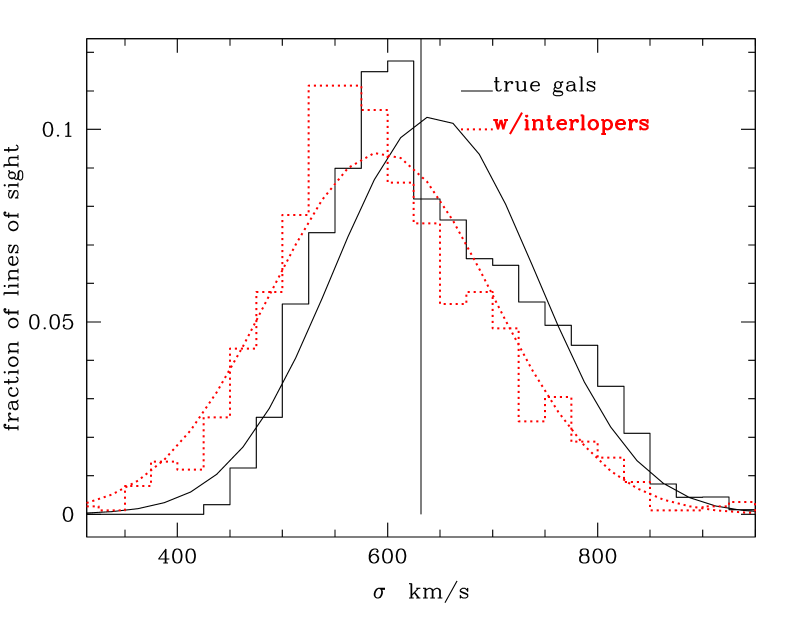
Figure 7: The composite histogram, normalized to unit area, of velocity dispersions for 10 clusters with $3\times 10^{14}\,h^{-1}M_{\odot}\leq M_{180b}\leq 3.5\times 10^{14}\,h^{-1}M_{\odot}$, in two cases: with only the true group members included (solid, black line, with 10,000 lines of sight per cluster) and with the full line-of-sight with interlopers removed as in §5 (red, dotted line, with 96 lines of sight per cluster). The curves indicate Gaussian fits. The vertical line at $\sigma\simeq 620\,{\rm km}/{\rm s}$ is the average of the three-dimensional velocity dispersions for these clusters. The line-of-sight measurement with interloper rejection has a lower average velocity dispersion (as seen also in van Haarlem et al., 1997; Biviano et al., 2006). Even this narrow range of halo masses exhibits a wide range of $\sigma$, as discussed in the text, with Gaussian fits of width $100\,{\rm km}/{\rm s}$. The skewness in the distribution is not present for all samples of this size.

As an example of an ensemble measurement, Fig. 7 shows the distribution of velocity dispersions measured from our simulation for 10 clusters with $3\times 10^{14}\,h^{-1}M_{\odot}\leq M_{180b}\leq 3.5\times 10^{14}\,h^{-1}M_{\odot}$. The solid histogram is the composite of $\sigma$ values for all the clusters, using the member galaxies only and projecting along 10,000 lines of sight for each cluster, while the line shows a Gaussian fit. (The dotted line and histogram are for the distribution which results when the same clusters are observed along 96 lines of sight, including interlopers and a culling method discussed below in §5).

This intrinsic line of sight scatter also suggests that if the goal is to determine the mass distribution there is an upper limit to the number of galaxy redshifts per cluster it is desirable to obtain: there is little to be gained by reducing sources of error in $\sigma_{\rm los}$ significantly below the dispersion above. Figure 8, which shows the velocity dispersion as a function of the number of subhalos used (added in order of decreasing luminosity), gives an illustration of this. Only subhalos which are within the friends-of-friends halo are included. All of the measures converge to a stable value for large numbers of subhalos, but the value depends significantly on the chosen line-of-sight. We find the number of subhalos at which the asymptotic limit is reached, and whether that approach is from above or below, depends upon the cluster under consideration, but the results are generally stable once 50 subhalos are included (Fig. 9).

Figure 8: The line-of-sight velocity dispersion vs. the number of subhalos included (ordered by $M_{\rm inf}$, i.e. luminosity, from highest to lowest) for a halo with $z\simeq 0.1$ mass $4\times 10^{14}\,h^{-1}M_{\odot}$. We include only subhalos which lie within the friends-of-friends halo, excluding any interlopers. The solid line shows the isotropic dispersion (i.e. $\sigma_{3D}/\sqrt{3}$) while the dotted and dashed lines show the dispersion along the eigenvector directions corresponding to the smallest and largest eigenvalues of $\sigma^{2}_{ij}$.

Figure 9: As in Fig. 8, the line-of-sight velocity dispersion vs. the number of subhalos included (ordered by $M_{\rm inf}$ from highest to lowest), but now for a range of halos and focusing on the region $N_{\rm sub}\leq 50$. As before, we include only subhalos which lie within the friends-of-friends halo, excluding any interlopers, and plot the line-of-sight dispersion normalized by the dispersion of the dark matter within the friends-of-friends halo. Note that each line converges to a stable result for large numbers of subhalos but the value depends upon the cluster and line-of-sight chosen, as does whether the approach is from above or below.

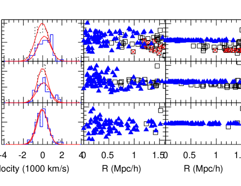
Figure 10: Line of sight histograms for the same massive $(M_{180b}=2.4\times 10^{14}\,h^{-1}M_{\odot})$ cluster along three different lines of sight. (Left) velocity histograms for all galaxies within $r_{180b}$ in plane of sky (dotted) and true cluster members (solid). The smooth curves are Gaussians with the same area under the curve as the line of sight velocity distributions, and with dispersion fit to the core of the line of sight velocity distribution to guide the eye. (Center) observed phase space diagram, transverse radius vs. redshift space position (including peculiar velocities). Solid (blue) triangles are true cluster members, open squares are interlopers from halos with mass $<0.2\,M_{\rm clus}$ and squares with (red) crosses inside are interlopers from halos with mass $>0.2\,M_{\rm clus}$, i.e. massive neighbors. (Right) true phase space diagram, transverse radius vs. true line-of-sight position (absent peculiar velocities). The bottom row is for a sightline where there are only 3 nearby galaxies (out of 87) and all measures are within 50 per cent of the true mass, the middle row has many nearby galaxies, but none from massive halos and overpredicts the mass in both Compton distortion and weak lensing by at least 50 per cent, and the top row has nearby galaxies from a nearby massive halo, about $10\,h^{-1}$Mpc in the foreground, and overpredicts the mass from lensing, velocity dispersions and Compton distortion. None of these lines of sight have appreciable substructure using the Dressler-Shechtman test described in §4.3.

Fig. 10 shows some typical line-of-sight velocity histograms and phase-space distributions for a massive ($M_{180b}=2.4\times 10^{14}\,h^{-1}M_{\odot}$) cluster viewed down three different lines-of-sight, with the solid lines being the histogram for the galaxies found within $r_{180b}$, i.e. the “true” cluster members. There is a large variation in the velocity dispersion profiles, even when only true members are included. The interloper structure seen will be discussed in §5.

4.3 Substructure

Figure 11: The persistence of substructure. The tracks show a small subset of the subhalos which fell into a large halo in the simulation as part of a large group at $z\simeq 0.3$, corresponding to the last major merger for this halo. Each panel is $6\,h^{-1}$Mpc on a side, centered on the $z=0$ position of the most bound particle in the halo, and the dashed line marks the virial radius ($r_{200c}$) of the main halo. To avoid crowding only a small fraction of the subhalos, the main progenitors with $M_{\rm inf}>10^{12}\,h^{-1}M_{\odot}$, are plotted. Subhalos which merge with these halos before $z=0$, and any subhalos which were not part of this group back at $z\simeq 0.3$ are omitted. Note the coherence of this “group of subhalos” for $3\,h^{-1}$Gyr.

Our massive halos contain significant substructure in both physical and velocity space, which is frequently attributed to the active merger histories of massive halos. We find that groups of subhalos which fall in together remain highly correlated for significant spans of time (several Gyr). In many respects these past accretion or merger events are still “ongoing”, in that the 3D density field has multiple distinct maxima and one can still see kinematically distinct groups of subhalos which were part of the merger partner and fell in together at that time. One example is given in Fig. 11, which shows the tracks of a small subset of the subhalos in a massive cluster and illustrates the long-term coherence of the group of subhalos even as it moves within the virial radius of its host. Though they are not highlighted in the figure, there are several other major groupings of subhalos that were accreted together and have survived for some time. Each has had a complex merger history but shows a long term persistence even though it is now well inside the formal virial radius of the host halo. It is an over-simplification to assume that when a halo falls into a larger neighbor and becomes a satellite that all its satellites become associated with the larger halo and evolve independently.

Not only do halos survive as distinct entities but groups of subhalos do as well. In fact, for massive halos, 30% of the subhalos in our sample are satellites when they fall in. One consequence of this has been seen in other contexts: satellites often merge with other satellites (rather than the central galaxy of their current halo), and the satellite they merge with is often the old central of the halo they were in prior to the merger (Angulo et al, 2009; Simha et al, 2009; Wetzel, Cohn & White, 2009). Visually we also saw correlated velocities between nearby satellites with different originating groups, presumably due to infall along a common filament. This long-term dynamical coherence also indicates that care should be taken when assuming relative velocities between galaxies are a substantial fraction of the host virial velocity, e.g. when estimating merger rates or impulses.

All of our simulated clusters have very obvious substructure. We have implemented several standard tests for dynamical substructure, which have been frequently applied to simulations and observed clusters in the literature, to see how well they find the substructure we know to be there. An excellent review of these methods can be found in Pinkney et al. (1996); some more recent statistics are summarized in Hou et al. (2009). We focus on the three dimensional test of Dressler & Shectman (1988), and the one dimensional tests of Kolmogorov and Arnold-Darling described in Hou et al. (2009) and refer the reader to papers there for details. The Dressler & Shectman (1988) test has been applied to simulations previously (e.g. Cen, 1997; Knebe & Muller, 2000), but usually to a large subset of the dark matter particles in the cluster rather than subhalos. Because we use subhalos identified with galaxies within the simulation, our methods are a further step in quantifying the difficulty of identifying cluster substructures observationally. When dark matter particles are used the large number available allows them to trace the cluster structure more faithfully than the observationally available galaxies, but using random dark matter particles as sample galaxies misses the dynamical coherence of groups of substructures that naturally arises in hierarchical structure formation scenarios.

We find many of our clusters show signs of substructure along some lines of sight: surprisingly, we find none of the three substructure indicators is well correlated with the time since last major merger, and the values of the indicators are very dependent on viewing angle for a given cluster even before we consider interlopers due to projection. If the substructure is well separated along the line-of-sight, from the bulk of the galaxies, then it is caught by each of the indicators. Otherwise it can be missed. As an example we pick one cluster, containing 57 subhalos brighter than $M_{\star}+1$. When viewed down the $z$-axis it is not flagged as having substructure by the tests we consider: the probability-to-exceed for the Dressler-Shectman test is 54 per cent, $D^{\star}=1.18$ and $A^{2\star}=1.68$ (Hou et al. (2009) suggest that $D^{\star}$ in excess of 1.2 or $A^{2\star}$ in excess of 1.9 indicate the presence of substructure). However, viewing this same cluster down the $x$-axis the probability-to-exceed for Dressler-Shectman is 3 per cent, $D^{\star}=2.76$ and $A^{2\star}=10$. There are many similar examples. In some cases the Dressler-Schechtman test flags substructure where the other tests do not, while for others the situation is reversed. Sometimes the Dressler-Shectman $\Delta$ statistic is high, but similar or larger values are obtained when shuffling the velocities (as described in Dressler & Shectman, 1988) leading to a higher probability-to-exceed or a lower significance detection of substructure. In these cases the prevalence of substructures in the host halo means that the “shuffled” statistics are not faithfully representing the “no substructure” scenario, leading one to erroneously assume the observed value of the statistic is consistent with no substructure.

These results suggest caution when interpreting lack of observed substructure in the galaxy distribution as evidence for a dynamically relaxed, steady-state object (e.g. justifying the use of the virial theorem or Jeans analysis without the time derivative). A cluster can be undergoing substantial mass accretion, i.e. be far from steady state, and still not be seen to have substructure along some lines of sight. The viewing angle dependence also complicates inferences about incidence of dynamical evolution of cluster galaxies from observed interactions of subclusters within the cluster identified through substructure finding techniques. There are some indications (e.g. Biviano et al., 1996; Adami et al., 2005) that more sophisticated substructure finding techniques could yield more complete information in the limit of hundreds of spectroscopic redshifts per cluster. Since we found earlier that the dynamics of the subhalos approached that of the dark matter particles as we progressed down the subhalo mass function, we expect very minor differences with earlier work when hundreds of subhalos are included.

5 Interlopers

The intrinsic line-of sight scatter in velocity dispersion discussed above (§4.2) is a “best case” estimate, where we have perfect identification of cluster members. In observations, an extra complication is provided by “interloper” galaxies which lie close to the cluster in the plane of the sky and in velocity but which nevertheless are really members of a different halo. Restricting samples to elliptical galaxies or matching on photometric properties can help, but does not solve the problem completely. Conversely, measurement errors in the velocities (which we do not model) can exacerbate the interloper problem – though it is expected that typical velocity errors will have only a small effect on estimates (Biviano et al., 2006).

Returning to Fig. 10, we now turn attention to the interlopers in the line-of-sight velocity histograms. In the middle and right columns we see the galaxies in phase space and physical space with true members represented by filled triangles, interlopers represented by open boxes and interlopers from massive halos (with mass $>0.2\,M_{\rm clus}$) represented by open boxes with crosses in them. Depending upon the line of sight, the same cluster can have (top to bottom): contributions from nearby massive halos, contributions only from less massive halos, or few interlopers. In these three instances the inferred red-sequence richness is very high, high and close to the mean for a cluster of this mass. It is typical that a single halo exhibits each of these characteristics when viewed from different directions, as a large fraction of halos have a massive neighbor. For the ensemble of velocity dispersions in our sample, while the distributions can often be well fit by a Gaussian profile, a non-trivial fraction of the lines-of-sight lead to “flat topped”, skew or bi-modal distributions or distributions that can be fit with Gaussians plus an excess in the wings (as seen in observations, e.g. Milvang-Jensen et al., 2008). In some cases interlopers cause an excess in the center of the velocity distribution.

5.1 Interloper removal

Several techniques have been devised to identify and reject these interlopers. Since in the simulations we know which objects are true cluster members we can apply these algorithms to our samples to see how they perform. Such investigations have been done before (e.g. Perea et al., 1990; den Hartog & Katgert, 1996; van Haarlem et al., 1997; Cen, 1997; Diaferio et al., 1999; Łokas et al., 2006; Wojtak et al, 2007, 2009) but typically using randomly selected dark matter particles rather than subhalos. By using subhalos we keep any correlations between subhalo positions and large-scale environment or between subhalos which fell in together as part of a larger structure. Including the interlopers in our mock observations and then using observational techniques to attempt to remove them is also important for estimating the scatter induced by the cosmic web, a main concern of this paper.

One of the simplest, and most widely used, interloper rejection methods is $3\,\sigma$ clipping (Yahil & Vidal 1977; Łokas et al. 2006; it has been applied in some large surveys and individual objects of special interest such as Halliday et al. 2004; Gal & Lubin 2004; Becker et al. 2007; Milvang-Jensen et al. 2008; Kurk et al 2009), which uses the fact that line-of-sight velocities of cluster members are close to Gaussian and iteratively excludes all galaxies $3\,\sigma$ away from the mean. Given enough galaxies one can perform this procedure in bins of transverse radius. Perea et al. (1990) developed a method based on removing galaxies whose absence causes the largest change in a mass estimator while Diaferio & Geller (1997) proposed the use of caustics and Prada et al. (2003) proposed an escape velocity cut. Various authors argue that the ‘gaps’ in the velocity distribution give a better rejection criterion (Zabludoff et al. 1990, Katgert et al. 1996,Owers, Couch & Nulsen 2009). Methods which use both projected coordinates and velocity information were introduced by den Hartog & Katgert (1996); Fadda et al. (1996).

We tested a number of interloper rejection algorithms. Here we focus on an example of the more complex methods which uses projected coordinates and velocity information (see e.g. den Hartog & Katgert, 1996; Biviano et al., 2006; Wojtak et al, 2007, and references therein), and its comparison to simple $3\,\sigma$ clipping. Such comparisons have been performed before (van Haarlem et al., 1997; Wojtak et al, 2009) but usually using randomly selected particles from lower resolution simulations rather than subhalos. Again this means that correlations between observed galaxy properties are more faithfully tracked in our case.

Our implementation is as follows. We assume that a trial center of the cluster has been determined. All galaxies with velocities within $3,000\,$km/s of the central velocity and projected radius smaller than $r_{180b}$ are then selected. The weighted gap method (e.g. Girardi et al., 1993) is then used to further remove galaxies along the line-of-sight. Specifically, gaps are defined as $g_{i}=v_{i+1}-v_{i}$ for the sorted velocities and weights as $w_{i}=i(N-i)$, for $i=1,\ldots,N-1$ for $N$ galaxies. Galaxies to one side of a weighted gap larger than 3 are removed, where the weighted gap is defined as

$$\frac{\sqrt{g\cdot w}}{MM(\sqrt{g\cdot w)}}\;,$$ (5)

with the midmean of the weighted gaps defined as

$$MM(\sqrt{g\cdot w})=\frac{2}{N}\sum_{N/4}^{3N/4}\sqrt{g\cdot w}\quad.$$ (6)

The motivation for such a cut lies in the expectation that the velocity dispersion is Gaussian, and the assumption that when the galaxy distribution departs from a Gaussian “core” it is no longer associated with the halo of interest. We use a modification to the weighted gap as described by Owers, Couch & Nulsen (2009), where it is applied separately in annuli of 50 galaxies each. Otherwise, we found the weighted gap tended to throw out too many galaxies.

Now we use the projected distribution to define a further, transverse radius dependent, velocity cut and iteratively remove galaxies beyond this cut. The cut depends on the (projected) harmonic radius, defined as

$$R_{h}^{-1}\equiv\frac{2}{N(N-1)}\sum_{i<j}R_{ij}^{-1}\quad,$$ (7)

where the sum is over galaxies out to radius $R$. If the velocity dispersion of the currently remaining galaxies is $\sigma$, we define a circular velocity as

$$v_{c}^{2}(R)=3\pi\ \sigma(R)^{2}\ \frac{R_{h}(R)}{R}\quad.$$ (8)

Typically $R_{h}/R\approx 1/2$ and decreases from center to edge, as the profile becomes steeper. From $v_{c}$ we further define a “freefall” velocity, $v_{ff}=\sqrt{2}\,v_{c}$. Then a galaxy at (projected) radius $R$ is an interloper if it is further from the cluster center than

$$v_{\rm max}(R)={\rm max}\left[v_{ff}(R)\cos\theta,v_{c}(R)\sin\theta\right]$$ (9)

where $\theta$ is the angle between radial vector and the line-of-sight and the maximization is done over the (real-space) line-of-sight position of the galaxy (the idea being that any observed galaxy can either be on a circular or radial orbit, with different boundedness criteria). Finally the velocity dispersion of the remaining galaxies is estimated using the bi-weight estimator described in Beers et al. (1990), and we shall refer to this as $\sigma_{\rm kin}$.

Though there is a wide diversity in cluster behaviors, the method of interloper rejection is more important than the precise dispersion estimator. The use of the on-sky positions to define a transverse radius dependent velocity cut performs slightly better than a fixed threshold, but in both cases the threshold varies significantly from step to step and can remove true cluster members while keeping actual interlopers.

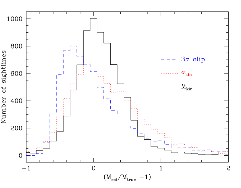
Figure 12: The distribution of mass predictions for the ensemble of sightlines for our massive sample using $3\,\sigma$ clipping, $\sigma_{\rm kin}$ and $M_{\rm kin}$ as described in the text. The areas under the curves differ because extreme outliers extend beyond the x-axis range shown. The “virial” mass, $M_{\rm kin}$, is the best tracer of the true mass.

Fig. 12 compares results from $3\,\sigma$ clipping and our more complex, phase-space based interloper rejection scheme for a sample of massive clusters. Except for extreme outliers, where the phase-space method performs slightly better, the distributions are quite close and noticeably non-Gaussian. These results are quite insensitive to cluster mass.

The more complex algorithm can fail in some instances. We found the most sensitive step was the weighted gap measurement, which can fail when the interloper structure along the line of sight is too close to define a clear gap in the velocity histogram. This is the case, for example, when two clusters are fairly close in one line of sight or when we see a chain of small substructures close together, as one would expect when looking down a filament. In these cases the weights given to the gaps do not work properly and gaps are not properly detected.

Once we include line-of-sight projections and the need for interloper removal, there is some gain to having more galaxies in order to better estimate the cluster potential (Fig. 13) but the intrinsic scatter due to the velocity ellipsoid remains a fundamental limitation (e.g. Fig. 7). As the number of galaxies with which we estimate the dispersion increases the estimate becomes stable but is still a relatively poor estimate of the angle-averaged dispersion.

Figure 13: As in Figs. 8 and 9, the line-of-sight velocity dispersion, (in units of the isotropically averaged dispersion for all subhalos) as a function of number of subhalos used, but now including non-member subhalos and using the interloper rejection scheme described in the text. The $x$-axis gives the number of subhalos used to compute the dispersion, after interloper removal. We have plotted 3 lines-of-sight for halos with $M_{180b}$ in the range $(0.6-1.0)\times 10^{15}\,h^{-1}M_{\odot}$.

5.2 Degradation due to interlopers

Applying this technique to our clusters, along 96 lines of sight each, allows us to find and compare the distributions of $\sigma$ values resulting from interlopers (and their rejection as described above) and the distribution due to intrinsic line of sight variation. The dotted line in Fig. 7 shows the distribution of $\sigma_{\rm kin}$ for the 96 sightlines for 10 clusters in mass range $(3-3.5)\times 10^{14}\,h^{-1}M_{\odot}$. The standard deviation in $\sigma_{\rm kin}$ is about $100\,{\rm km}/{\rm s}$ when only cluster member galaxies are included and is approximately 10 per cent larger when including (and then rejecting) interlopers. There is a slight downward shift in the mean $\sigma_{\rm kin}$, as was also seen by Biviano et al. (2006). These trends are reproduced for higher and lower mass clusters.

The line-of-sight dispersion is only one piece of information available to estimate masses, and other information can be introduced. For example, one can include the compactness of the cluster, estimated from the projected member positions, or go further including corrections for surface terms and orbital anisotropy, and beyond. It is not our intention here to model each of the (complex) methods which have been presented in the literature, but we do note that the next-to-simplest suggested mass estimator is proportional to $\sigma_{\rm kin}^{2}R_{h}$ where $R_{h}$ is the (projected) harmonic radius of Eq. (7). We shall denote this $M_{\rm kin}$. Formally this estimator would be valid only for spherical, isolated systems with galaxies tracing mass, but due to a correlation between errors in $R_{h}$ and $\sigma$ we find $M_{\rm kin}$ produces a tighter, less skewed estimate of $M_{180b}$ than the pure dispersion based measures (see Fig. 12) even in our more complex systems. Although there is some variation from cluster to cluster, most often a higher-than-average $\sigma$ is compensated by a lower-than-average $R_{h}$. The compensation is not perfect, but it reduces the significance of the fluctuation, leading to more lines-of-sight within the core of the distribution and fewer strong outliers. (Similar cancellations were seen by Biviano et al. (2006) when comparing observations with and without interlopers. They found the tendency of interlopers to bias $\sigma$ low was (over-)compensated by their tendency to bias $R_{h}$ upwards.) For this reason it is $M_{\rm kin}$ which we correlate with other quantities in the following section.

We also note that Biviano et al. (2006) found a correlation between catastrophic outliers in the mass-$\sigma_{\rm kin}$ or mass-$M_{\rm kin}$ relations and substructure. Using the Dressler-Shectman test on the galaxies which were selected using our interloper rejection procedure we found that 39 per cent of the lines of sight had substructure ($P<0.05$) and of these only 10 per cent had $>50$ per cent deviations between $M_{\rm kin}$ and true mass. By contrast, of the lines-of-sight with $>50$ per cent deviation in $M_{\rm kin}$, 52 per cent had substructure to be compared to 40 per cent for lines-of-sight where $M_{\rm kin}$ is a reliable estimate of mass. Thus outliers in $M_{\rm kin}$ do tend to have detectable substructure more often than non-outliers, but substructure doesn’t necessarily lead to $M_{\rm kin}$ outliers and thus is not a reliable flag for it.

6 Multiwavelength measures: correlated scatter

Although clusters obey tight scaling relations, we expect a large scatter in individual measures of cluster mass/size. Clusters are generally triaxial and highly biased. They are formed and fed at the intersection of a network of filaments in atypical and anisotropic cosmological environments. Their mass accretion is punctuated by a series of mergers with other massive objects. With the growing number of multi-wavelength, large area surveys underway multiple measurements of large numbers of clusters are possible, and there is a hope that different methods can cross-check each other.

As scatter is often caused by the cosmic web, measures sensitive to the web will have correlations induced in their scatter. Consider an idealized model, in which galaxies flow into the cluster from a small number of (approximately straight) filaments, retaining memory of this due to incomplete virialization. In such a scenario, we might expect the line-of-sight component of the velocities is biased for the same viewing angles as those for the projected mass, projected pressure and projected galaxy number density. This would lead to correlations in the mass inferred by richness, dynamics, Compton distortion and lensing. In this section we consider the relative strengths of these correlations and their causes in the local cluster environment.

6.1 Basic results

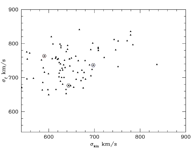
Figure 14: Correlated scatter for an individual cluster between velocity dispersion $\sigma_{\rm kin}$ and lensing dispersion $\sigma_{\zeta}$. The circles correspond to the three lines of sight shown in Fig. 10 for the same cluster. Of the three, the lowest lensing dispersion corresponds to the bottom panel there (with hardly any nearby interlopers), the largest lensing dispersion (and lowest $\sigma_{\rm kin}$) corresponds to the center panel with many low mass neighbors, and the largest velocity dispersion corresponds to the top panel, with a high mass nearby halo. The isotropic velocity dispersion for this cluster is 690 km/s.

Considering richness, dynamics, lensing and Compton distortion, we found that the degree of correlation between different measures of cluster size varied dramatically from cluster to cluster, each sampling a different, local, cosmic web. Taking the median covariances from all the massive clusters the largest covariances were between red galaxy richness and all other quantities, followed by covariances of velocity dispersion with the other probes. In terms of scatter of $M_{\rm pred}/M_{\rm true}-1$, the tightest correlations with mass in our measures was for Compton distortion and phase space richness, followed by weak lensing, and then red galaxy richness and velocity dispersion. We show in Fig. 14 the measures of lensing dispersion and velocity dispersion along all 96 lines of sight for the same cluster as in Fig. 10: a correlation can be seen.

The correlations between individual measurements were usually below $0.5$, indicating that each additional observation is adding significant new information about the mass/size of the cluster, with the lower dispersion measures giving the tightest constraints. It should be borne in mind though that the distributions were far from Gaussian, and the mass function steeply falling, so errors should be interpreted with care.

To compare the ensemble of multiwavelength measurements for all the lines of sights for all the clusters, we fit mean power-law relations between the observables and mass to convert each multiwavelength measure to a common system (the “predicted” mass). Then we divided up the sightlines into “good” and “bad” based on whether $|(M_{\rm true}-M_{\rm pred})|/M_{\rm true}\geq 0.5$ for at least 2 independent observables. The bad sightlines comprised 8 (11) per cent of the 96 sightlines per cluster with $M\geq 2(1)\times 10^{14}\,h^{-1}M_{\odot}$. Over half of the massive ($M\geq 2\times 10^{14}\,h^{-1}M_{\odot}$) clusters had at least one sightline where at least 3 measures were off (the most common sources of mass errors were in red galaxy richness, velocity dispersion and lensing), and more than half of the bad sightlines were due to 18/83 of the clusters, each with 10 or more bad sightlines. As $\sim 1/3$ of the sightlines had at least one quantity giving more than a 50 per cent error from the mean mass relation, the reduction in error to 8 per cent of the sightlines when using at least two measures is a significant improvement. Using only galaxies with $L\geq 0.4\,L_{\star}$ (rather than $L\geq 0.2\,L_{\star}$) resulted in a small increase in the number of bad sightlines (from 8 to 11 per cent).

Scatter in the observables can arise from several violations of the idealized, isolated, relaxed, spherical halo assumption. The halo itself can be irregular (e.g. recently merged), or regular but anisotropic. Nearby correlated material can be seen in projection or uncorrelated material at large distances can be projected onto the cluster position. We have discussed halo state and anisotropy above. Here our interest is in the comparison of nearby structure and substructure for bad and good lines of sight. We considered a cluster to have nearby massive structure if at least three $L\geq 0.4\,L_{\star}$ galaxies from another halo(s) of mass $\geq 0.2\,M_{\rm cluster}$ were present within $3\,\sigma_{\rm kin}$ in redshift space and within $r_{180b}$ in the plane of the sky, and to have nearby less massive structure if nearby massive structure wasn’t present as above and at least eight $L\geq 0.4\,L_{\star}$ galaxies from halos with mass $\leq 0.2\,M_{\rm cluster}$ were within the same region. For halos above $2\times 10^{14}\,h^{-1}M_{\odot}$ we found 21 per cent of the bad sightlines had nearby massive structure and 49 per cent had nearby less massive structure, compared to 2 and 25 per cent respectively for the good sightlines. The bad sightlines were 10 times more likely to have a nearby massive halo and almost twice as likely to have nearby less massive halos. A larger fraction (52 per cent) of the bad sightlines have cluster substructure (Dressler-Shechtman probability less than 0.05 as described in §4.3), compared to 38 per cent of the good sightlines. All together, 80 per cent of the bad sightlines had one of these three indicators (nearby massive structure, or numerous less massive structure, or substructure) compared to 51 per cent of the good sightlines. These numbers changed very little when we lowered the mass threshold to $10^{14}h^{-1}M_{\odot}$.

However, although the likelihood of substructure, nearby massive or less massive halos increased for bad sightlines, the majority of sightlines with substructure, nearby massive or less massive halos were not bad sightlines. Of the 39 per cent of the lines of sight which have substructure detected, only 10 per cent are bad lines of sight. Similarly of the 4 per cent of sightlines with nearby massive structure, 59 per cent are good, and 41 per cent are bad. For the 26 per cent with nearby less massive structure, 86 per cent are good and 14 per cent are bad.

6.2 Implications for stacking

As is well known, correlated errors must be handled with care. For example, if the source of scatter is correlated, two non-independent measures can agree and both be in error. These subtleties must also be borne in mind then one starts to stack measurements (see also Nord et al., 2008; Rykoff et al, 2008; Stanek et al., 2010).

Stacking can be done in several ways. Multiple measurements can be made for a set of objects and then the mean of one of the measurements can be taken holding another fixed. Alternatively, there may be insufficient signal to measure all of the properties on individual objects, so they are first stacked on one property and the second is measured on the stack. In this case one has the additional freedom to either scale the size of any aperture with the first property or use a fixed metric aperture. Finally, one can relate two properties while holding a third property fixed either by averaging individual methods or measuring the properties on an average (e.g. fix richness and then measure Compton distortion and lensing).

It is known that a scatter between two variables, $x$ and $y$, implies that conditional probabilities must be interpreted with care. For example, there is scatter between halo mass, $M$, and richness, $N$, which in the mean obey a relation lg$M=a+b\,{\rm lg}N$. However the mean (log) mass of halos in a bin $N\approx N_{0}$ is not $a+b\,{\rm lg}N_{0}$. Since there are typically many more low mass halos than high mass halos, it is likely that a high richness object is in reality a low mass object with artificially high richness for its mass rather than an intrinsically massive object of mean (or low) richness. The degree of such bias depends on the amount of scatter and the slope of the halo mass function, which becomes steeper at both high mass and high redshift. If one estimates the mass using a method (e.g. lensing) which itself has scatter, then the degree of error also depends on how correlated the scatter between these methods is and the relative sizes of the scatter.

For example, if scatter in richness were driven entirely by line-of-sight projection of nearby structures, and if it was identical to the amount of mass projected onto the “lens”, then the error in the mass estimated by lensing would cancel the bias described above. However, if one measures an extra property, e.g. X-ray flux, which is immune to the projection, the mass–flux relation one infers from the stack would be biased to high masses at fixed flux. This would lead to an incorrect relation between mass and X-ray flux. For detailed formulae in a simple analytical model see Appendix C (and Rykoff et al, 2008; Nord et al., 2008).

In general we expect the situation to be slightly more complicated in reality (or simulations) than the log-normal, analytical model suggests. We saw in the last section that a small number of halos are responsible for a fair fraction of the outliers, and that the distribution of errors has non-Gaussian tails. While the general trends are not altered by these issues, they serve to alter the quantitative predictions.

In fact none of these complications lead to large corrections to our measured scaling relations. All of the quantities show strong trends with mass, and all of them have relatively large scatter. The distribution of points in the observable–observable plane is therefore determined by the range of masses being selected much more than subtle correlations between the observables. This serves to make any biases relatively small. While we fully expect biases to be present, given our limited simulation volume we are not able to measure them reliably.

Some examples serve to illustrate the main points. We choose as a fiducial sample all lines-of-sight with red-sequence richness $29\leq N\leq 30$ at $z\simeq 0.1$, containing 271 lines-of-sight from 104 halos. We choose red-sequence richness as it is one of the more common quantities to stack on. As expected, the mean mass of these clusters is skewed low by the steeply falling mass function. The line-of-sight weighted mean mass is $M_{180b}\simeq 2.2\times 10^{14}\,h^{-1}M_{\odot}$. A randomly chosen sample of halos with the same mass distribution has a line-of-sight weighted mean richness of 22-24 (with fluctuations depending on how the sampling is done), i.e. it is $\sim 25$ per cent poorer than the input sample. The mean (and median) values of the velocity dispersion, projected mass and Compton distortion of this random sample are also “low”. How do these mean values compare to those of the sample selected on richness? In fact they are quite similar, differing by $<10$ per cent in the mean. This is because there is a large degree of scatter between red sequence richness and mass and a strong correlation of all measures with mass, making selecting on richness approximately the same as randomly sampling halos with a specific mass distribution. The joint distributions of e.g. Compton distortion and velocity dispersion or projected mass and Compton distortion also turn out to be very similar in the random- and richness-selected samples. There is a tendency for the richness-selected sample to have more outliers in velocity dispersion using $3\sigma$ clipping than the random sample, but otherwise the joint distributions are almost indistinguishable.

We find similar results by stacking on e.g. velocity dispersion. The distribution in e.g. the $Y-\zeta$ plane is the same for the velocity dispersion selected sample as in a sample of the same mass distribution.

The largest impact of stacking on e.g. richness for our sample then is not the degree to which the scatters in individual measurements are correlated on an object-by-object basis but the fact that the stack contains clusters of a wide range of masses/sizes. If the measurement being performed is a non-linear function of the mass, care must be taken in interpreting the meaning of the averaged quantity.

7 Higher redshift

Unfortunately our simulation volume is too small to make robust statements about increasingly rare objects at high redshift, but in this section we note some trends. According to Moster et al. (2010) the lower mass limit of our subhalos corresponds to lower stellar-mass subhalos at higher $z$, with the limit dropping from $3\times 10^{9}\,h^{-1}M_{\odot}$ at $z\simeq 0$ to $2\times 10^{9}\,h^{-1}M_{\odot}$ at $z\simeq 0.5$ to $1\times 10^{9}\,h^{-1}M_{\odot}$ at $z\simeq 1$. There is little evolution in the characteristic stellar mass in the mass function over the same range, so we probe further below the break in the mass function at higher $z$. Since, on average, satellite subhalos fell into their host more recently at higher $z$, the satellite fraction is smaller for samples selected above a given halo mass or stellar mass (see discussion in e.g. Wetzel & White, 2010).

While we have 83 halos with $M\geq 2\times 10^{14}\,h^{-1}M_{\odot}$ at $z\simeq 0.1$, this drops to 28 at $z\simeq 0.5$ and only 5 at $z\simeq 1$, making us increasingly susceptible to “outliers”. The number of massive neighbors per very massive halo increases as we go to higher $z$, due to the steepening of the mass function at the high-mass end. Though the statistics are poor, there is evidence that the velocity bias of the subhalos is decreasing with increasing redshift (see also Evrard et al., 2008). The distribution of the eigenvalues of the velocity ellipsoid is very similar to that at $z\simeq 0.1$ (shown in Fig. 5), again leading to large changes in line-of-sight velocity dispersion with viewing angle.

At $z\simeq 0.5$ we found again that $M_{\rm kin}\propto R_{h}\sigma^{2}$ was more tightly correlated with halo mass than $\sigma^{3}$, as it was at $z\simeq 0.1$. The more complex, phase-space interloper rejection method continued to perform better than pure $3\,\sigma$ clipping. In fact the trends of errors and correlations between mass and phase space richness, Compton distortion, projected mass and velocity dispersion were unchanged. The phase-space richness and Compton distortion had the least dispersion, followed by projected mass and then galaxy kinematics. The fraction of bad sightlines does not change substantially going from $z\simeq 0.1$ to $z\simeq 0.5$, however the fraction of these bad sightlines with many interlopers from low-mass halos decreases. As expected from the increasing halos biases at higher redshift, the distribution of number of halos around the massive clusters tended to have a higher mean at higher redshift. The substructure fraction between $z=0.1$ and $z=0.5$ was close to unchanged.

8 Conclusions

Advances in observational capabilities and a new generation of wide-field surveys have led to an explosion in multi-wavelength samples of galaxy clusters. By studying a cluster in many different wavebands, and from many different approaches, we can obtain complementary information about the physical state of the clusters and mitigate the systematic errors in any single measurement. Combining different measurements of cluster properties has to be done carefully however, because the environment in which clusters form leads to features which can be correlated across methods. As the correlation is not perfect, such a combination will provide improvements over any individual method if done correctly.

In this paper we have used high resolution N-body simulations of a cosmological volume to study how the large-scale environment of clusters leads to correlated scatter in measures of cluster size, specifically those based upon richness, Compton distortion, lensing or velocity dispersions. Our simulation has enough force and mass resolution to track the subhalos which are expected to host galaxies, allowing us to study dynamical probes of the cluster with realistic samples incorporating a hierarchy of substructures and retaining correlations between subhalo positions, velocities and environment. For this reason we paid particular attention to dynamical probes of cluster size.

As might be expected in hierarchical structure formation scenarios, groups of subhalos retain their identity for long periods within larger host halos. This leads to a “lack of virialization” which implies that substructures can thus behave quite coherently in phase space. The highly anisotropic nature of infall into massive clusters, and their triaxiality, means that line-of-sight galaxy velocity dispersions (or virial masses) for any individual halo show large variance depending on viewing angle. This suggests that dispersion-based mass estimators will work better in an ensemble sense than for any individual cluster and that obtaining more than tens of redshifts for any given cluster will not reduce the inferred mass error. We discussed the effect interloper galaxies, and their removal, has on kinematic measurements and compared different schemes for interloper removal. Results were presented both for individual clusters and for a “stacked” ensemble cluster.

All of our simulated clusters contain highly evident substructure, with groups of subhalos which fall in together moving in a coherent fashion for several Gyr. However standard substructure indicators frequently miss this substructure, and often give very different answers for a single object viewed from different directions. These results suggest caution when interpreting lack of observed substructure in the galaxy distribution as evidence for a dynamically relaxed, steady-state object (e.g. justifying the use of the virial theorem or Jeans analysis without the time derivative). A cluster can be undergoing substantial mass accretion, i.e. be far from steady state, and still not be seen to have substructure along some lines of sight. The viewing angle dependence also complicates inferences about incidence of dynamical evolution of cluster galaxies from observed interactions of subclusters within the cluster identified through substructure finding techniques.

Finally we note that many observational probes of clusters suffer from projection effects, and that these are exacerbated by the dense, active and anisotropic environments surrounding these massive objects. We found increased nearby massive and less massive halos, and substructure, when two of our measures (richness, lensing, Compton distortion and velocity dispersions) simultaneously had large outliers in predicted mass. The converse was not always true, scatter in environment or the measurement of substructure did not necessarily imply large outliers.

Since the orientation of the velocity ellipsoid is correlated with the large-scale structure, velocity outliers also correlate with projection induced outliers. For many cases the same structure causes scatter in different observations: such scatters can be substantially correlated and this correlation needs to be properly incorporated when combining measurements.

We would like to thank J. Bullock, A. Evrard, B. Gerke, H.Hoekstra, E. Rozo, E. Rykoff, C. Stubbs, A. Wetzel and A. Zabludoff for conversations and A. Evrard and A. Wetzel for comments on the draft. We thank A. Zabludoff for suggesting we consider the “virial mass” $R_{h}\sigma^{2}$ in addition to $\sigma^{3}$. M.W. thanks Charlie Conroy and James Gunn for useful conversations and collaborations about the stellar population synthesis technique. We thank the referee, Andrea Biviano, for a constructive report and helpful suggestions. The simulations used in this paper were performed at the National Energy Research Scientific Computing Center and the Laboratory Research Computing project at Lawrence Berkeley National Laboratory. M.W. was supported by the DoE and NASA. R.S. was supported by the University of California Education Abroad Program. J.D.C. thanks LBNL for travel support to the SNOWCLUSTER meeting and thanks its organizers and participants for the opportunity to present this work and for their suggestions and questions.

Appendix A Finding subhalos

In our past work we have used the Subfind algorithm (Springel et al., 2001) to find subhalos. However we have found that a phase-space based approach performs better at tracking the subhalos in our most massive hosts and for this reason we have switched to this new scheme here. In particular we follow Diemand, Kuhlen & Madau (2006) and implement a phase-space friends-of-friends finder. Detailed experimentation, including a one-to-one comparison of the new finder with the results of Subfind, suggest that choosing the configuration-space linking length to be $0.078$ of the mean interparticle spacing and the velocity linking length to be $e^{-1}\simeq 0.368$ of the halo (1D) velocity dispersion gives a good subhalo catalog. As discussed in Diemand, Kuhlen & Madau (2006) the results are stable to modest changes in these parameters. The most massive subhalos are the same for both finders, but the lower mass structures which pass close to the center of the halo are more robustly tracked in the phase-space method than with Subfind. We keep all 6D FoF halos which contain more than 20 particles. For technical, book-keeping reasons if fewer than two subhalos (i.e. a central and a satellite) are found in any host halo we slowly increase the linking lengths in that halo until one or two subhalos are found. This ensures that there are no low-mass halos which have no subhalos, simplifying the book-keeping in the tracking scheme. This affects only the very low mass halos which are not used in this paper.

Appendix B The red sequence

It has become common to use the tight red sequence of galaxies found in clusters in order to isolate putative cluster members from chance alignments along the line-of-sight during cluster detection. The evolution of the red sequence with redshift means that choosing red galaxies within a certain color cut also tends to give galaxies at a certain redshift. Because color-based cluster finders have become so popular, we have included a toy-model of a color-based richness in our mocks. There are two steps, first to assign colors to the mock galaxies and second ask how the observed properties depend on redshift/distance. We take each of these in turn.

B.1 Color assignment

We first put colors into our $z\simeq 0.1$ box using the method of Skibba & Sheth (2009). Their approach has red and blue galaxy populations being drawn from two different populations (each with an $M_{r}$-dependent mean and scatter), where the probability of a galaxy belonging to either population depending upon $M_{r}$ and whether it is a central or satellite galaxy.

We associate $r$-band magnitude with infall mass by abundance matching, ignoring any scatter in the $M_{r}-M_{\rm inf}$ relation for simplicity. Skibba & Sheth (2009) approximate the probability of a satellite to be red as

$$P_{\rm sat}(M_{r})=\frac{\langle g-r|M_{r}\rangle_{\rm sat}-\langle g-r|M_{r}\rangle_{\rm blue}}{\langle g-r|M_{r}\rangle_{\rm red}-\langle g-r|M_{r}\rangle_{\rm blue}}$$ (10)

where

$$\begin{array}[]{lll}\langle g-r|M_{r}\rangle_{\rm sat}&=&0.83-0.08(M_{r}+20)\\ \langle g-r|M_{r}\rangle_{\rm red}&=&0.93-0.03(M_{r}+20)\\ \langle g-r|M_{r}\rangle_{\rm blue}&=&0.62-0.11(M_{r}+20)\end{array}$$ (11)

and find an overall red fraction

$$f_{\rm red}(M_{r})\simeq 0.54-0.07(M_{r}+20)\quad.$$ (12)

Given $P_{\rm sat}(M_{r})$, $f_{\rm red}$ and $f_{\rm sat}$ one can solve for $P_{\rm cen}(M_{r})$, see Table 1. One then takes every galaxy, satellite or central, and randomly decides whether it is red or blue. If needed its actual color can be taken from the Gaussian fits to the color-magnitude relations given by Skibba & Sheth (2009).

lg$M_{\rm inf}$	$M_{r}$	$f_{\rm red}$	$P_{\rm cen}$	$P_{\rm sat}$
11.50	-19.1	0.48	0.41	0.62
12.00	-20.2	0.56	0.50	0.69
12.50	-20.9	0.60	0.56	0.76
13.00	-21.4	0.64	0.60	0.83
13.50	-21.8	0.67	0.63	0.91

Table 1: Magnitudes and red fractions as a function of infall mass (in $h^{-1}M_{\odot}$) from Skibba & Sheth (2009). $f_{\rm red}$ is the fraction of all galaxies which are red, while $P_{\rm cen}$ and $P_{\rm sat}$ are the probabilities that a central or satellite galaxy of that infall mass is red.

B.2 Evolution with redshift

The fact that the observed colors of galaxies evolve with distance means that a tight sequence in color (e.g. the red sequence) will shift out of any thin color slice as the galaxies shift in distance. Thus cuts in color can be used to isolate galaxies within a small range of distances (e.g. Gladders & Yee, 2000, 2005). Modeling the evolution of galaxy colors ab initio is notoriously difficult, but a hybrid method based on stellar population synthesis models can isolate the main features for our purposes of making “pseudo” light cones.

We simplify our problem by assuming that blue galaxies can be distinguished from red at any distance and we need only consider the evolution of the red galaxies. We make the further simplification that all of the red galaxies are evolving passively, with star formation having ceased at some high redshift (e.g. $z\geq 2$). Using the stellar population models described in (Conroy, Gunn & White, 2009; Conroy, White, & Gunn, 2010; Conroy, & Gunn, 2010) we find that the $g-r$ color of a passively evolving population scales with redshift as $d(g-r)/dz\simeq 1$–2, with the precise slope depending on the star formation history assumed. Similarly, the absolute $r$-band magnitude scales as $dM_{r}/dz\simeq 0.1$–1. For our cosmology $d\chi/dz=2900\,h^{-1}$Mpc, where $\chi$ is the (comoving) line-of-sight distance and a linear approximation is acceptable over the limited extent of our simulation.

Given a color cut of a certain width the speed at which the color of the red sequence “ridgeline” changes with $z$ defines the range of distance over which galaxies will be selected. We encode this information as the probability that a red galaxy at a given distance will fall into the fiducial red sequence cut (c.f. Cohn et al., 2007).

If the width and peak of the red sequence were independent of the magnitude this transformation would be trivial: for a Gaussian color distribution and a fixed width $\Delta c$ the interloper probability is the difference of two error functions with width $\Delta c/(dc/d\chi)$. However the non-zero dependence on $M_{r}$ slightly complicates the calculation. To include this complication we first calculate the corresponding magnitude for every red galaxy as if it were actually at redshift $0.1+\delta z$, corresponding to its offset from the box midplane, but dimmed (or brightened) by the change in distance. We then calculate what $M_{r}$ and thus $g-r$ distribution will result for this dimmed galaxy as it evolved to $z=0.1$, assuming the linear evolution defined above. The evolved $M_{r}$ at $z=0.1$ has a $z=0.1$ color ($g-r$) distribution well fit by a Gaussian distribution (Skibba & Sheth, 2009). The color is evolved back to $z=0.1+\delta z$ to give the observed color distribution for the galaxy at $z=0.1+\delta z$ with magnitude $M_{r}$ estimated as if it were at $z=0.1$. The interloper fraction of galaxies is the integral of the observed distribution within the cut defining the red sequence.

If we make our red sequence selection have $g-r$ width 0.05 we find the dispersion in distance runs between $50$ and $100\,h^{-1}$Mpc, depending on stellar population model, galaxy magnitude etc. To be conservative, in the sense of reducing line-of-sight projection, we take the lower end of the range and assume a red galaxy in the foreground or background of the cluster of interest is included within the red sequence with a Gaussian probability of width $50\,h^{-1}$Mpc. As with the other measures, we apodize the selection to ensure the probability is zero at the limits of the simulation.

Appendix C Measurements with correlated scatter and stacking

It is helpful to consider a simple analytic model which illustrates the effect of correlated scatter on different observables. We will consider the case of two measurements, $m_{1}$ and $m_{2}$, of some quantity $m$. For example, one could consider $m_{1}$ to be richness-inferred (log) mass and $m_{2}$ to be lensing-inferred (log) mass with $m$ the “true” (log) mass. We imagine that $P(m_{1},m_{2}|m)$ is a bi-variate Gaussian with means $\mu_{i}(m)$ and covariance

$${\rm Cov}\left[m_{1},m_{2}\right]=\left\{\begin{array}[]{cc}\sigma_{1}^{2}&\rho_{12}\sigma_{1}\sigma_{2}\\ \rho_{12}\sigma_{1}\sigma_{2}&\sigma_{2}^{2}\\ \end{array}\right\}\quad.$$ (13)

and for simplicity we assume that $\sigma_{i}$ and $\rho_{12}$ are independent of $m$ and that $\mu_{i}=a_{i}+b_{i}m$. We shall write the probability that a cluster has mass $m$, the mass function, as $P(m)$ and for convenience/simplicity take it to be a power-law in mass or $P(m)\propto\exp[-\alpha m]$.

As is well known, when $\sigma_{i}>0$ and $\alpha\neq 0$ the mean “true” mass of clusters with measured mass $m_{i}$ is biased. Since $P(m|m_{1})\propto P(m_{1}|m)P(m)$ we have

$$\left\langle m|m_{1}=m_{1}^{\rm obs}\right\rangle\equiv\bar{m}=\frac{m_{1}^{\rm obs}-a_{1}}{b_{1}}-\frac{\alpha}{b_{1}^{2}}\,\sigma_{1}^{2}\quad.$$ (14)

Similarly, if we consider the case where $m_{1}$ is known (e.g. selected) to be $m_{1}^{\rm obs}$ the conditional distribution of $m_{2}$ is also a Gaussian with $\sigma_{2}^{\prime}=(1-\rho_{12}^{2})\sigma_{2}^{2}$ and mean

$$\left\langle m_{2}|m_{1}=m_{1}^{\rm obs},m\right\rangle=\mu_{2}+\frac{\sigma_{2}}{\sigma_{1}}\rho_{12}\ \left(m_{1}^{\rm obs}-\mu_{1}\right)\quad.$$ (15)

These facts allow us to consider computing $m_{2}$ as a function of $m$ by binning on $m_{1}$ and averaging the measures of $m_{2}$ in each bin. It is easy to show that if $\sigma_{1}=0$ one simply obtains $\langle m_{2}\rangle=a_{2}+b_{2}\bar{m}=a_{2}+(b_{2}/b_{1})(m_{1}^{\rm obs}-a_{1})$ as desired. However if the $\sigma_{i}>0$ we have more terms. By writing $P(m_{1},m_{2},m)=P(m_{2}|m,m_{1})P(m|m_{1})P(m_{1})$ and recalling that the $\mu_{i}$ are linear in $m$ one finds Eq. (15) with $\mu_{i}(\bar{m})$ in place of $\mu_{i}(m)$ leading to

$$\left\langle m_{2}\right\rangle=a_{2}+\frac{b_{2}}{b_{1}}\left(m_{1}^{\rm obs}-a_{1}\right)+\frac{\alpha}{b_{1}}\left(\rho_{12}\sigma_{1}\sigma_{2}-\frac{b_{2}}{b_{1}}\sigma_{1}^{2}\right)\,.$$ (16)

Consider the case $a_{i}=0$ and $b_{i}=1$, i.e. the measurements give unbiased estimates of the (log) mass for halos of a fixed mass: $\left\langle m_{i}|m\right\rangle=m$. Stated another way, the average of each mass estimate in narrow bins of halo mass returns the correct mass and in such bins each measurement correctly predicts the mass which would be estimated by every other measurement. If one could bin in mass, it would be straightforward to estimate the mean observable-mass relation.

The situation changes when we bin not by mass but by observable, e.g. richness. In this case, even though the richness-based mass estimator is unbiased, the (unobservable) true mean halo mass in the bin is biased (low) because the falling mass function makes it more likely that a halo of richness $N$ is a low mass halo which fluctuated up than a high mass halo which fluctuated down in richness. Similarly, the mean mass estimated from a second observable in that bin differs by $\alpha(\rho_{12}\sigma_{1}\sigma_{2}-\sigma_{1}^{2})$ from the first observable defining the bin, as in Eqn.  16. That observable-mass relation is thus also biased. Note that the bias disappears if $\rho=1$ and $\sigma_{1}=\sigma_{2}$, in which case the errors conspire to cancel exactly because fluctuations in observable one directly imply compensating fluctuations in observable two. For example, a low mass halo which had an abnormally high richness would be counted in the richness bin even when it “should not be”. But its lensing signal would also be abnormally high by just the right amount to give the right mean mass in the richness bin.

Finally, if we estimate a third observable in the same bins of e.g. richness it will be biased by a different amount: $\alpha(\rho_{13}\sigma_{1}\sigma_{3}-\sigma_{1}^{2})$. The relation between observables $2$ and $3$, when binned on $1$, is thus biased in both coordinates. Though we have not considered it in our toy model, this bias may well be mass dependent.

In these examples the bias is due entirely to the falling mass function, because we assumed explicitly that $a_{i}=0$ and $b_{i}=1$, i.e. the measurements give unbiased estimates of the mass. Using the results above, the general case can be considered but we gain no further insight from doing so.

References

- Abell (1958) Abell G.O., 1958, ApJS, 3, 211
- Adami et al. (2005) Adami, C., Biviano, A., Durret, F., Mazure, A., 2005, A&A, 443, 17
- Angulo et al (2009) Angulo R.E.; Lacey C.G., Baugh C.M., Frenk C.S., 2009, MNRAS, 399, 983
- Bhattacharya et al. (2010) Bhattacharya S., Heitmann K., White M., Lukic Z., Wagner C., Habib S., 2010, ApJ, submitted.
- Becker et al. (2007) Becker M.R., et al., 2007, ApJ, 669, 905
- Beers et al. (1990) Beers T.C, Flynn K., Gebhardt K., 1990, AJ, 100, 32
- Biviano et al. (1996) Biviano, A., Durret, F., Gerbal, D., Le Fevre, O., Lobo, C., Mazure, A., Slezak, E., 1996, A&A, 311, 95
- Biviano et al. (2006) Biviano, A., Murante, G., Borgani, S., et al. 2006, A&A, 456, 23
- Blanton et al. (2003) Blanton M., et al., 2003, ApJ, 592, 819
- Bohringer et al. (2000) Bohringer H., et al., 2000, ApJS, 129, 435
- Bohringer et al. (2001) Bohringer H., et al., 2001, A&A, 369, 826
- Boylan-Kolchin et al. (2009) Boylan-Kolchin M., Springel V., White S.D.M., Jenkins A., Lemson G., 2009, MNRAS, 398, 1150
- Cohn & White (2009) Cohn J.D., White M., 2009, MNRAS, 393, 393
- Cohn et al. (2007) Cohn J.D., Evrard A.E., White M., Croton D., Ellingson E., 2007, MNRAS, 382, 1738
- Conroy & Ostriker (2008) Conroy C., Ostriker J., 2008, ApJ, 681, 151
- Conroy, Gunn & White (2009) Conroy C., Gunn J.E., White M., 2009, ApJ, 699, 486
- Conroy, White, & Gunn (2010) Conroy C., White M., Gunn J.E., 2010, ApJ, 708, 58
- Conroy, & Gunn (2010) Conroy C., Gunn J.E., 2010, ApJ, 712, 833
- Cen (1997) Cen R., 1997, ApJ, 485, 39
- Crone, Evrard & Richstone (1996) Crone M.M., Evrard A.E., Richstone D.D., 1996, ApJ, 467, 489
- Dalton et al (1992) Dalton, G.B., Efstathiou, G., Maddox, S.J., & Sutherland, W.J., 1992, ApJL 390, L1
- Davis et al. (1985) Davis M., Efstathiou G., Frenk C.S., White S.D.M., 1985, ApJ, 292, 371
- den Hartog & Katgert (1996) den Hartog, R., Katgert, P., 1996, MNRAS, 279, 349
- Diaferio & Geller (1997) Diaferio A., Geller M.J., 1997, ApJ, 481, 633
- Diaferio et al. (1999) Diaferio A., Kauffmann G., Colberg J.M., White S.D.M., 1999, MNRAS, 307, 537
- Diemand, Kuhlen & Madau (2006) Diemand J., Kuhlen M., Madau P., 2006, ApJ, 649, 1
- Dressler & Shectman (1988) Dressler A., Shectman S.A., 1988, AJ, 95, 985
- Evrard et al. (2008) Evrard A.E., et al., 2008, ApJ, 672, 122
- Faber et al. (2007) Faber S., et al., 2007, ApJ, 665, 265
- Fadda et al. (1996) Fadda D., Girardi M., Giuricin G., et al., 1996, ApJ, 473, 670
- Faltenbacher (2010) Faltenbacher A., 2010, preprint [arxiv:0912.0013]
- Faltenbacher & Diemand (2006) Faltenbacher A., Diemand J., 2006, MNRAS, 369, 1698
- Faltenbacher et al. (2009) Faltenbacher A., Li C., White S.D.M., Jing Y.-P., DeMao S., Wang J., 2009, RAA, 9 41
- Gal & Lubin (2004) Gal, R.R., Lubin, L., 2004, ApJL 607, 1
- Gao et al. (2004) Gao L., de Lucia G., White S.D.M., Jenkins A., 2004, MNRAS, 352, L1
- Girardi et al. (1993) Girardi M., Biviano A., Giuricin G., Mardirossian F., Mezzetti M., 1993, ApJ, 404, 38
- Gladders & Yee (2000) Gladders M., Yee H.K.C., 2000, AJ, 120, 2148
- Gladders & Yee (2005) Gladders M., Yee H.K.C., 2005, ApJS, 157, 1
- Goto (2005) Goto, T., 2005, MNRAS, 359, 1415
- Halliday et al. (2004) Halliday, C., et. al., 2004, A&A, 427, 397
- Hallman et al (2007) Hallman, E.J., O’Shea, B.W., Burns, J.O., Norman, M.L., Harkness, R., Wagner, R., 2007, ApJ 671, 27
- Heitmann et al. (2008) Heitmann K., et al., 2008, CS&D, 1, 15003
- High et al (2010) High, F.W., et al., 2010, preprint arxiv:1003.0005
- Hoekstra (2001) Hoekstra H., 2001, A&A, 370, 743
- Hoekstra, Yee & Gladders (2002) Hoekstra H., Yee H., Gladders M., 2002, New Astronomy Reviews, 46, 767
- Holder, McCarthy & Babul (2007) Holder, G.P., McCarthy, I.G., Babul, A., 2007, MNRAS 382, 1697
- Hou et al. (2009) Hou A., Parker L., Harris W., Wilman D., 2009, ApJ, 702, 1199
- Jenkins et al. (2001) Jenkins, A., Frenk, C. S., White, S. D. M., Colberg, J. M., Cole, S., Evrard, A. E., Couchman, H. M. P., & Yoshida, N. 2001, MNRAS, 321, 372
- Jiang, Jing & Lin (2010) Jiang, C. Y., Jing, Y. P., Lin, W. P., 2010, A&A, 510, A60
- Jing & Suto (2002) Jing Y.P., Suto Y., 2002, ApJ, 574, 538
- Kaiser (1986) Kaiser N., 1986, MNRAS, 222, 323
- Kasun & Evrard (2005) Kasun S.F., Evrard A.E., 2005, ApJ, 629, 781
- Katgert et al. (1996) Katgert P., Mazure A., Perea J., et al., 1996, A& A, 310, 8
- Kazantzidis et al (2004) Kazantzidis, S., Kravtsov, A.V., Zentner, A.R., Allgood, B., Nagai, D., Moore, B., 2004, ApJ, 611, L73
- Knebe & Muller (2000) Knebe A., Muller V., 2000, A&A, 354, 761
- Koester et al. (2007) Koester B.P., et al., 2007, ApJ, 660, 221
- Kurk et al (2009) Kurk, J., et al., 2009, A&A, 504, 331
- Lau, Nagai & Kravtsov (2010) Lau E.T., Nagai D., Kravtsov A.V., 2010, ApJ, 708, 1419
- Lin, Mohr & Stanford (2004) Lin Y.T., Mohr J.J., Stanford S.A., 2004, ApJ, 610, 745
- Łokas et al. (2006) Łokas E.L., Wojtak R., Göttlober S., et al., 2006, MNRAS, 367, 1463
- Lumsden et al (1992) Lumsden, S.L., Nichol, R.C., Collins, C.A., Guzzo, L., 1992, MNRAS 258,1
- McHardy (1978) McHardy I., 1978, MNRAS, 184, 783
- Meneghetti et al. (2010) Meneghetti, M., Fedeli, C., Pace, F., Gottloeber, S., Yepes, G., 2010, arXiv:1003.4544
- Metzler, White & Loken (2001) Metzler C., White M., Loken C., 2001, ApJ, 547, 560
- Milvang-Jensen et al. (2008) Milvang-Jensen, B., et al., 2008, A&A, 482, 419
- Moster et al. (2010) Moster B., et al., 2010, MNRAS, 710, 903 [arxiv:0906.0764]
- Navarro, Frenk & White (1997) Navarro J.F., Frenk C.S., White S.D.M., 1997, ApJ, 490, 493
- Nord et al. (2008) Nord, B., Stanek, R., Rasia, E., Evrard, A.E., 2008, MNRAS, 383L, 10
- Owers, Couch & Nulsen (2009) Owers, M.S., Couch, W.J., Nulsen, P.E.J., 2009, ApJ, 693, 901
- Perea et al. (1990) Perea J., del Olmo A., Moles M., 1990, A&A, 237, 319
- Pinkney et al. (1996) Pinkney J., Roettiger K., Burns J.O., Bird C.M., 1996, ApJS, 104, 1
- Prada et al. (2003) Prada F., Vitvitska M., Klypin A., et al., 2003, ApJ, 598, 260
- de Putter & White (2005) de Putter R., White M., 2005, New Astronomy, 10, 676
- Reblinsky & Bartelmann (1999) Reblinsky K., Bartelmann M., 1999, A&A, 345, 1
- Refregier (2003) Refregier A., 2003, ARA&A, 41, 465
- Robertson et al. (2009) Robertson B., Kravtsov A.V., Tinker J., Zentner A.R., 2009, ApJ, 696, 636
- Rykoff et al (2008) Rykoff, E.S., et al., 2008, MNRAS Letters, 387, 28
- Schwartz (1978) Schwartz D.A., 1978, ApJ, 220, 8
- Shaw, Holder & Bode (2008) Shaw, L.D., Holder, G.P., Bode, P., 2008, ApJ, 686, 206
- Simha et al (2009) Simha, V., Weinberg, D. H., Dave, R., Gnedin, O. Y., Katz, N., Keres, D., 2009, MNRAS, 399, 650
- Siverd, Ryden & Gaudi (2010) Siverd R.J., Ryden B.S., Gaudi B.S., 2010, preprint [arxiv:0903.2264]
- Skibba & Sheth (2009) Skibba R.A., Sheth R.K., 2009, MNRAS, 392, 1080
- Springel et al. (2001) Springel V., White S.D.M., Tormen G., Kauffmann G., 2001, MNRAS, 328, 726
- Stanek et al. (2010) Stanek, R., Rasia, E., Evrard, A.E., Pearce, F., Gazzola, L., 2010, MNRAS, 403, 1072
- Staniszewski et al. (2009) Staniszewski Z., et al., 2009, ApJ, 701, 32
- Sunyaev & Zel’dovich (1972) Sunyaev R.A., Zel’dovich Ya.B., 1972, Comments on Astrophysics and Space Physics, 4, 173
- Thomas & Couchman (1992) Thomas, P. A., Couchman, H. M. P., 1992, MNRAS 257, 11
- Tormen (1997) Tormen G., 1997, MNRAS, 290, 411
- van der Marel et al. (2000) van der Marel R.P., Magorrian J., Carlberg R.G., et al., 2000, AJ, 119, 2038
- van Haarlem et al. (1997) van Haarlem M.P., Frenk C.S., White S.D.M, 1997, MNRAS, 287, 817
- Warren et al (1992) Warren, M.S., Quinn, P.J., Salmon, J.K., Zurek, W.H., 1992, ApJ, 399, 405
- Weinmann et al (2009) Weinmann, S.M., Kauffmann, G., von der Linden, A., De Lucia, G., 2009, arXiv:0912.2741
- Wetzel, Cohn & White (2009) Wetzel A., Cohn J.D., White M., 2009, MNRAS, 395, 1376
- Wetzel (2010) Wetzel A., 2010, submitted to MNRAS, [arxiv:1001.4792]
- Wetzel & White (2010) Wetzel A., White M., 2010, MNRAS, 403, 1072
- White et al (1999) White, R., et al 1999, AJ 118, 2014
- White (2001) White M., 2001, A&A, 367, 27
- White (2002) White M., 2002, ApJS, 143, 241
- White, Hernquist & Springel (2002) White, M., Hernquist, L., Springel, V., 2002, ApJ, 579, 16
- Wittman et al. (2006) Wittman D., et al., 2006, ApJ, 643, 128
- Wojtak et al (2007) Wojtak, R., Lokas, E.L., Mamon, G.A.,Gottlober,S., Prada F., Moles M., 2007, A&A 466, 437
- Wojtak et al (2009) Wojtak, R., Lokas, E.L., Mamon, G.A.,Gottlober,S., 2009, MNRAS 399, 812
- Yahil & Vidal (1977) Yahil, A, Vidal, N.V., 1977, ApJ, 214, 347
- Yang, Mo & van den Bosch (2008) Yang X., Mo H.J., van den Bosch F.C., 2008, ApJ, 676, 248
- Zabludoff et al. (1990) Zabludoff A. I., Huchra J.P., Geller M.J., 1990, ApJ, 74, 1
- Zwicky et al. (1966) Zwicky F., Herzog E., Wild P., 1966, “Catalog of galaxies and of clusters of galaxies”, Vol. 3 (Pasadena: California Institute of Technology).