Hidden parameters in open-system evolution unveiled by geometric phase

Abstract

We find a class of open-system models in which individual quantum trajectories may depend on parameters that are undetermined by the full open-system evolution. This dependence is imprinted in the geometric phase associated with such trajectories and persists after averaging. Our findings indicate a potential source of ambiguity in the quantum trajectory approach to open quantum systems.

I Introduction

Closed quantum systems evolving deterministically under some Hermitian Hamiltonian is an idealized description that at best approximates real laboratory experiments. In fact, all quantum systems undergo open-system effects induced by entanglement with environmental degrees of freedom; effects that may be detrimental in various quantum information protocols in which coherence is an essential ingredient nielsen00 . This feature has led to a revived interest in the theory of open quantum systems and how to deal with open-system effects by different types of error control to achieve error resilient quantum information processing shor95 .

Geometric and holonomic quantum computation, first conceived in Ref. zanardi99 and experimentally demonstrated in Ref. jones00 , is an approach to error control that has attracted considerable attention recently. In its simplest variant, it makes use of the Abelian geometric phase berry84 to construct quantum logical gates acting on one or two quantum mechanical bits (qubits) ekert00 . These gates may be used to build quantum Boolean networks and may be combined with other error resilient methods to perform robust quantum computation wu05 ; oreshkov09 . The need to understand the error resilience of geometric and holonomic quantum computation has led to proposals for the geometric phase of open quantum systems carollo03 ; tong04 ; marzlin04 ; sarandy06 .

Here, we examine the idea in Ref. carollo03 (see also Ref. carollo04a ) to associate geometric phases of individual quantum trajectories in quantum jump unravelings of Lindblad-type open-system evolution plenio98 . This approach involves only pure state geometric phases, which may relate to the geometry of the full open-system evolution by some averaging over trajectories sjoqvist06 .

The trajectory-based geometric phase simplifies the analysis of the robustness of geometric and holonomic quantum computation cen04 ; fuentes05 ; moller08 . The idea is that for weak influence of the environment, it suffices to consider the lowest order, no-jump trajectory to evaluate error resilience. Here, we show that this geometric phase may in certain cases lead to different predictions regarding the resilience of geometric and holonomic quantum computation to open-system effects. This result indicates a potential source of ambiguity in the no-jump approach to analyze weak open-system effects.

The problem of how to define open-system geometric phases by averaging over quantum trajectories has been addressed in Refs. bassi06 ; buric09 . These works employ quantum state diffusion (QSD) gisin92 , which is a form of stochastic unravelings of the Lindblad evolution consisting of continuous, Brownian-type trajectories in state space.

In Ref. bassi06 , the averaged geometric phase associated with the full nonlinear form of the QSD equation gisin92 was examined. It was found that this phase is not invariant under unitary rotations $L_{m}\rightarrow\sum_{n}V_{mn}L_{n}$ of the Lindblad operators $L_{m}$. On the other hand, Ref. buric09 demonstrated that this noninvariance would disappear if the averaged geometric phase is instead associated with the linearized version of QSD goetsch94 , provided the system starts in a pure state. Based on this result, it was claimed in Ref. buric09 that the linearized QSD approach provides a uniquely defined geometric phase of open systems. Here, we demonstrate the existence of a class of Markovian open-system evolutions for which the linearized QSD geometric phase may change under symmetry transformations of the full Lindblad evolution.

The outline of the paper is as follows. In the next section, we find symmetry transformations of a certain class of Markovian open-system evolutions which are not symmetries of the corresponding no-jump trajectories. These transformations are shifts of the Lindblad operators, i.e., of the form $L_{m}\rightarrow L_{m}-f_{m}(t)\hat{1}$. Here, $f_{m}(t)$ are arbitrary complex-valued functions and are hidden parameters in the sense that they do not affect this class of Markovian evolution models. In Sec. III, this result is illustrated by an explicit calculation of the no-jump geometric phase for a dephasing qubit (spin$-\frac{1}{2}$) being exposed to a static magnetic field. The geometric phase for stochastic unravelings in the form of the linearized QSD equation is analyzed in Sec. IV. The paper ends with the conclusions.

II Shift symmetries of open-system evolutions

We consider Markovian evolution of open quantum systems governed by the Lindblad equation ($\hbar=1$ from now on) lindblad76

$$\dot{\rho}(t) = -i[H(t),\rho(t)]+\left.\lambda\sum_{m}\right(L_{m}\rho(t)L_{m}^{\dagger}$$ (1)

$$\left.-\frac{1}{2}L_{m}^{\dagger}L_{m}\rho(t)-\frac{1}{2}\rho(t)L_{m}^{\dagger}L_{m}\right)$$

$$= -i[H(t),\rho(t)]+\lambda\mathcal{L}(\rho(t)).$$

Here, $L_{m}$ are dimensionless Lindblad operators that model the influence of the environment on the system evolution. For simplicity, we shall assume that $L_{m}$ are time-independent. The parameter $\lambda\geq 0$ controls the strength of the open-system effect, such that $\lambda=0$ corresponds to unitary closed system evolution.

The Lindblad equation obeys certain symmetries; an apparent one is the independence of choice of zero point energy corresponding to the transformation $H(t)\rightarrow H(t)-h(t)\hat{1}$, where $h(t)$ is real valued and $\hat{1}$ is the identity operator. Another general type of symmetry corresponds to the transformation $L_{m}\rightarrow\sum_{n}V_{mn}L_{n}$, where $V_{mn}$ is an arbitrary unitary matrix buric09 . One may check that this transformation leaves the Lindblad equation unchanged and thus will not affect the state $\rho(t)$ of the system.

The quantum jump unraveling is defined by dividing the evolution given by Eq. (1) into small time steps $\Delta t$. In the $\Delta t\rightarrow 0$ limit, this procedure leads to quantum trajectories in state space consisting of smooth deterministic parts interrupted by random jumps, generated by jump operators proportional to $L_{m}$. For a pure initial state $\psi_{0}$, these trajectories reside in projective Hilbert space $\mathcal{P}(\mathcal{H})$ formed by rays of the system’s Hilbert space $\mathcal{H}$. These rays are equivalence classes consisting of vectors that differ by multiplication of nonzero complex numbers. As shown in Ref. carollo03 , one may associate a pure state geometric phase to each such trajectory. Here, we focus on the geometric phase of no-jump trajectories. Such a trajectory is the projection onto $\mathcal{P}(\mathcal{H})$ of the continuous Hilbert space path

$$[0,T]\ni t\rightarrow|\psi(t)\rangle={\bf T}e^{-i\int_{0}^{t}\widetilde{H}(t^{\prime})dt^{\prime}}|\psi_{0}\rangle$$ (2)

with ${\bf T}$ time ordering and

$$\widetilde{H}(t)=H(t)-\frac{i}{2}\lambda\sum_{m}L_{m}^{\dagger}L_{m}$$ (3)

a non-Hermitian effective no-jump Hamiltonian. The corresponding no-jump geometric phase acquired on the time interval $[0,T]$ reads carollo03

$$\gamma_{nj} = \arg\langle\psi(0)|\psi(T)\rangle+\int_{0}^{T}\frac{\langle\psi(t)|H(t)|\psi(t)\rangle}{\langle\psi(t)|\psi(t)\rangle}dt.$$ (4)

Note that $\gamma_{nj}$ is a property of a path in $\mathcal{P}(\mathcal{H})$ as it is invariant under the transformation $|\psi(t)\rangle\rightarrow c(t)|\psi(t)\rangle$ together with $H(t)\rightarrow H(t)+i\frac{d}{dt}\ln\frac{c(t)}{|c(t)|}$, where $c(t)$ is a nonzero complex number for all $t\in[0,T]$.

It is straightforward to check that the no-jump path $|\psi(t)\rangle$ and the corresponding geometric phase $\gamma_{nj}$ are unaffected by the above-mentioned unitary rotation $L_{m}\rightarrow\sum_{n}V_{mn}L_{n}$. But there may be other symmetries that apply only to certain classes of open systems. We focus on the symmetry related to the shifts $L_{m}\rightarrow L_{m}-f_{m}(t)\hat{1}$ where $f_{m}(t)$ is in general complex-valued. Such shifts induce the transformations

$$H(t) \rightarrow K(t)=H(t)-\frac{i}{2}\lambda\sum_{m}\left(f_{m}^{\ast}(t)L_{m}-f_{m}(t)L_{m}^{\dagger}\right),$$

$$\mathcal{L} \rightarrow \mathcal{L}.$$ (5)

Thus, they result solely in an extra term in the Hamiltonian part of Eq. (1). This implies that the Lindblad evolution is unchanged under the shifts of $L_{m}$ if all $f_{m}^{\ast}(t)L_{m}$ are Hermitian. In such a case, $f_{m}(t)$ are said to be hidden parameters of the full open-system evolution. On the other hand, the no-jump Hamiltonian transforms as

$$\widetilde{H}(t)\rightarrow\widetilde{K}(t) = \widetilde{H}(t)+\frac{i}{2}\lambda\sum_{m}\Big{(}f_{m}(t)L_{m}^{\dagger}$$ (6)

$$+f_{m}^{\ast}(t)L_{m}-|f_{m}(t)|^{2}\hat{1}\Big{)}$$

with $\widetilde{H}(t)$ the no-jump Hamiltonian in Eq. (3). The transformed no-jump Hamiltonian $\widetilde{K}(t)$ may be nontrivially different from $\widetilde{H}(t)$ even for Hermitian $f_{m}^{\ast}(t)L_{m}$. Thus, for shifts $L_{m}\rightarrow L_{m}-f_{m}(t)\hat{1}$ such that $f_{m}^{\ast}(t)L_{m}$ are Hermitian, the Lindblad evolution is unchanged but the deterministic no-jump evolution may undergo a nontrivial change originating from the anti-Hermitian contributions $\frac{i}{2}\lambda\left(f_{m}(t)L_{m}^{\dagger}+f_{m}^{\ast}(t)L_{m}\right)$ to $\widetilde{K}(t)$. In this case, the no-jump trajectories may depend on the parameters $f_{m}$, which are hidden in the full open-system evolution. We note that this result applies to any smooth portion of a quantum trajectory, i.e., trajectories that contain one or several jumps share with the no-jump trajectories the same kind of behavior under shifts of the Lindblad operators.

The $f_{m}$ dependence may be interpreted as an manifestation of a continuous monitoring of the environment in the presence of a specific form of system-environment interaction. To see this explicitly, let us consider a unitary representation model for the system-environment evolution during the time interval $[t,t+\delta t]$, where $\delta t$ is the finite time resolution for measuring projectively the environment in some orthogonal basis $\{|0_{e}\rangle,|m_{e}\rangle\}$. We assume that $\delta t$ and $\lambda$ are much smaller than the typical energy shift associated with $H(t)$. Under this assumption, the change in the system-environment state can be described by a unitary map $U(t,t+\delta t;\{f_{m}(t)\})$ with the effect

$$|0_{e}\rangle|\psi(t)\rangle \rightarrow U(t,t+\delta t;\{f_{m}(t)\})|0_{e}\rangle|\psi(t)\rangle$$

$$= |0_{e}\rangle\left(\hat{1}-i\widetilde{K}(t)\delta t\right)|\psi(t)\rangle$$

$$+\sqrt{\lambda\delta t}\sum_{m}|m_{e}\rangle\left(L_{m}-f_{m}(t)\hat{1}\right)|\psi(t)\rangle.$$

Here, we have assumed that the environment is prepared in the pure state $|0_{e}\rangle$ and we have taken

$$\langle 0_{e}|U(t,t+\delta t;\{f_{m}(t)\})|0_{e}\rangle = \hat{1}-i\widetilde{K}(t)\delta t,$$

$$\langle m_{e}|U(t,t+\delta t;\{f_{m}(t)\})|0_{e}\rangle = \sqrt{\lambda\delta t}\left(L_{m}\right.$$ (8)

$$\left.-f_{m}(t)\hat{1}\right)$$

to the first order in $\delta t$ and $\sqrt{\lambda\delta t}$. Thus, the shifts $L_{m}\rightarrow L_{m}-f_{m}(t)\hat{1}$ would correspond to engineering the system-environment interaction so that Eq. (8) is satisfied. Evidently, the jump operators are $\sqrt{\lambda\delta t}\left(L_{m}-f_{m}(t)\hat{1}\right)$. The no-jump trajectory $[0,T]\ni t\rightarrow|\psi(t)\rangle={\bf T}e^{-i\int_{0}^{t}\widetilde{K}(t^{\prime})dt^{\prime}}|\psi_{0}\rangle$ is realized with probability $\langle\psi(T)|\psi(T)\rangle$ by verifying that no change has occurred in the environment, and repeating up to time $T$.

The operators $F_{0}(t)=\hat{1}-i\widetilde{K}(t)\delta t$ and $F_{m}(t)=\sqrt{\lambda\delta t}\left[L_{m}-f_{m}(t)\hat{1}\right]$ in Eq. (8) constitute a set of Kraus operators that represent a completely positive map of system states from $t$ to $t+\delta t$. Provided all $f_{m}^{\ast}(t)L_{m}$ are Hermitian, there is a unitary matrix $\boldsymbol{W}(t)$ that relates this Kraus representation with the original one consisting of $E_{0}(t)=\hat{1}-i\widetilde{H}(t)\delta t$ and $E_{m}(t)=\sqrt{\lambda\delta t}L_{m}$. Explicitly, we may write $F_{\mu}(t)=\sum_{\nu}\boldsymbol{W}_{\mu\nu}(t)E_{\nu}(t)$, $\mu,\nu=0,1,\ldots$, with

$$\boldsymbol{W}(t)=\begin{pmatrix}1-\frac{1}{2}\lambda\delta t\sum_{m}\left|f_{m}(t)\right|^{2}&\sqrt{\lambda\delta t}f_{1}^{\ast}(t)&\sqrt{\lambda\delta t}f_{2}^{\ast}(t)&\sqrt{\lambda\delta t}f_{3}^{\ast}(t)&\ldots\\ -\sqrt{\lambda\delta t}f_{1}(t)&1&0&0&\ldots\\ -\sqrt{\lambda\delta t}f_{2}(t)&0&1&0&\ldots\\ -\sqrt{\lambda\delta t}f_{3}(t)&0&0&1&\ldots\\ \vdots&\vdots&\vdots&\vdots&\ddots\end{pmatrix},$$ (9)

which can be checked to be unitary to lowest order in $\delta t$ and $\sqrt{\lambda\delta t}$. The existence of such a unitary matrix demonstrates nielsen00 that the two maps are physically identical if all $f_{m}^{\ast}(t)L_{m}$ are Hermitian; a result that is consistent with the invariance of the Lindblad equation under the shifts $L_{m}\rightarrow L_{m}-f_{m}(t)\hat{1}$ for this type of open-system evolution.

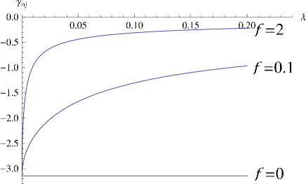
Figure 1: (Color online) The no-jump phase $\gamma_{nj}$ as a function of the open-system strength $\lambda$ for the shift values $f=0,0.2,2$. The initial state is taken to be pure on the equator ($\theta_{0}=\frac{\pi}{2}$) of the Bloch sphere. The horizontal curve for $f=0$ demonstrates the $\lambda$ independence found in Refs. carollo03 ; fuentes05 . For $f\neq 0$, $\gamma_{nj}$ depends strongly on $\lambda$.

III Geometric phase

We next show that the previous result may have consequences for the geometric phase of a no-jump trajectory. We find an explicit physical example where a shift parameter $f$ is imprinted in the no-jump geometric phase, although the corresponding open-system evolution is $f$-independent.

Consider a qubit (spin$-\frac{1}{2}$) prepared in the pure state $|\psi_{0}\rangle=\cos\left(\frac{1}{2}\theta_{0}\right)|0\rangle+\sin\left(\frac{1}{2}\theta_{0}\right)|1\rangle$, exposed to a static magnetic field in the $z$ direction and to dephasing of strength $\lambda$. This may be modeled by a Hamiltonian $H=\frac{\omega}{2}\sigma_{z}$ and a single Lindblad operator $L=\sigma_{z}$, with $\omega$ the precession frequency and $\sigma_{z}=|0\rangle\langle 0|-|1\rangle\langle 1|$ the $z$ component of the standard Pauli operators. By using Eqs. (5) and (6), we find the transformations $H\rightarrow K=H-\lambda\text{Im}(f)\sigma_{z}$, $\mathcal{L}\rightarrow\mathcal{L}$, and $\widetilde{H}\rightarrow\widetilde{K}=\widetilde{H}+i\lambda\text{Re}(f)\sigma_{z}-\frac{i}{2}\lambda|f|^{2}\hat{1}$, under the shift $L\rightarrow L-f\hat{1}$, where $f$ is assumed to be time-independent for simplicity. Thus, the Lindblad evolution is unaffected by the shift if $f$ is real-valued. On the other hand, the geometric phase of the no-jump trajectory

$$[0,T]\ni t\rightarrow|\psi(t)\rangle=e^{-i\widetilde{K}t}|\psi_{0}\rangle$$ (10)

for a quasi-cyclic path over the time interval $[0,2\pi/\omega]$ with real-valued $f$, takes the form

$$\gamma_{nj} = -\pi+\frac{\omega}{4f\lambda}\ln\left(e^{\frac{4\pi}{\omega}f\lambda}\cos^{2}\frac{\theta_{0}}{2}\right.$$ (11)

$$\left.+e^{-\frac{4\pi}{\omega}f\lambda}\sin^{2}\frac{\theta_{0}}{2}\right),$$

which is explicitly $f$-dependent.

The geometrical reason for this $f$-dependence can be seen by looking at the Bloch sphere polar angle $\theta$, which becomes time-dependent if $f\neq 0$. Explicitly, by evaluating the right-hand side of Eq. (10) we obtain $\tan[\theta(t)/2]=e^{-2f\lambda t}\tan(\theta_{0}/2)$ and azimuthal angle $\varphi(t)=\varphi_{0}+\omega t$, which correspond to a spiralling motion toward the north (south) pole of the Bloch sphere for $f>0$ ($f<0$) and all $\theta_{0}\neq\pi$ ($\theta_{0}\neq 0$). Furthermore, one may check that $\gamma_{nj}$ in Eq. (11) converges to the expected $-\pi(1-\cos\theta_{0})$ (minus half the solid angle enclosed on the Bloch sphere) in the $f\lambda\rightarrow 0$ limit. The nontrivial $f$ dependence is illustrated in Fig. 1. The resilience to dephasing of the geometric phase of the no-jump trajectory found in Refs. carollo03 ; fuentes05 corresponds to the case $f=0$. However, as our calculation shows, any nonzero $f$ would predict $\gamma_{nj}$ to be $\lambda$-dependent and thus be affected by this kind of open-system effect. For small $f\lambda$, this dependence is linear, which may be seen by expanding the geometric phase around the closed system expression, leading to the lowest order correction $2\pi^{2}\frac{f\lambda}{\omega}\sin^{2}\theta_{0}$.

We may show that the no-jump evolution of dephasing for $f\neq 0$ is equivalent to decay of the precessing qubit. Consider the evolution generated by the Lindblad operator $L_{-}=\sigma_{x}-i\sigma_{y}$, which corresponds to decay toward the south pole of the Bloch sphere with some strength $\lambda^{\prime}$, say. The no-jump curve is determined by the effective no-jump Hamiltonian $\widetilde{H}^{\prime}=\frac{\omega}{2}\sigma_{z}-i\lambda^{\prime}\sigma_{z}-i\lambda^{\prime}\hat{1}$, where we have assumed the Hamiltonian $H=\frac{\omega}{2}\sigma_{z}$. If $\lambda^{\prime}=-f\lambda$, then the no-jump Hamiltonian $\widetilde{H}^{\prime}$ generates the same curve in $P(\mathcal{H})$ as $\widetilde{H}$ in the dephasing model (the corresponding Hilbert space curves differ only by multiplication of a nonzero complex number).

It is instructive to compare the preceding dephasing example with the mixed state geometric phase $\gamma[\mathcal{P}]$ proposed in Ref. tong04 for real-valued $f$. Since $\gamma[\mathcal{P}]$ is based directly on the kinematics $\rho(t)$ of open-system evolution, it follows immediately that $\gamma[\mathcal{P}]$ is $f$-independent and therefore experimentally testable cucchietti10 . It was furthermore found that $\gamma[\mathcal{P}]$ for precession around the $z$ axis is resilient to dephasing only if the initial state lies on the equator of the Bloch sphere. This particular form of resilience has been reported in a recent experiment filipp09 with polarized ultracold neutrons exposed to dephasing noise.

For one-qubit systems, $f_{m}^{\ast}(t)L_{m}$ can be chosen to be Hermitian for all open-system models that include Lindblad operators that are linear combinations of the Pauli operators with real coefficients, such as dephasing and depolarization. On the other hand, it should be stressed that if no $f_{m}(t)$ exist such that $f_{m}^{\ast}(t)L_{m}$ becomes Hermitian, then the shift in fact corresponds to a new Hamiltonian that may cause a different evolution $\rho(t)$. One such example is spontaneous decay of a qubit, for which one cannot find a nonzero $f$ such that $f^{\ast}L_{-}$ becomes Hermitian. Indeed, the shift $L_{-}\rightarrow L_{-}-f\hat{1}$ induces the Zeeman term $\lambda\left[\text{Im}(f)\sigma_{x}+\text{Re}(f)\sigma_{y}\right]$ in the Hamiltonian, in the case of spontaneous decay. Another example is a spin$-\frac{1}{2}$ system interacting with a quantized light field and subjected to a linear loss of photons. This loss may be modeled by the non-Hermitian photon annihilation operator $L=a$. In this case, the shift $L\rightarrow L-f\hat{1}$ yields the extra term $\sqrt{2}\left[-\text{Im}(f)x+\text{Re}(f)p\right]$ in the Hamiltonian, where $x=(a+a^{\dagger})/\sqrt{2}$ and $p=(a-a^{\dagger})/(i\sqrt{2})$ are the ‘position’ and ‘momentum’ operators, respectively, of the quantized light field. It is reasonable to expect that any robustness in the geometric phase found in these two latter types of systems would signal an error resistance also at the level of the full Lindblad evolution. Applications of the quantum jump unraveling to these model systems have indeed shown a nontrivial error resilience cen04 ; carollo04b , results that support the usefulness of the geometric phase for robust quantum computation.

IV Stochastic unravelings

Stochastic unravelings in the form of quantum state diffusion (QSD) gisin92 consist of continuous, Brownian-like quantum trajectories whose average coincides with the full Lindblad evolution. The geometric phase of such trajectories arising from nonlinear gisin92 and linear goetsch94 versions of the QSD equation has been considered in Refs. bassi06 and buric09 , respectively. Reference bassi06 considered the phase transformation $L_{m}\rightarrow e^{i\chi_{m}}L_{m}$ and found a nontrivial $\chi_{m}$ dependence in the geometric phase for the nonlinear QSD evolution. In Ref. buric09 , it was demonstrated that the averaged geometric phase $\alpha_{g}$ associated with the linearized evolution is invariant under unitary rotations $L_{m}\rightarrow\sum_{n}V_{mn}L_{n}$, provided the system starts in a pure state. Here, we examine the behavior of this geometric phase under the shifts $L_{m}\rightarrow L_{m}-f_{m}(t)\hat{1}$ and show that $\alpha_{g}$ may depend on $f_{m}$, also when $f_{m}$ is hidden in the full open-system evolution.

The linearized QSD equation reads

$$|d\phi\rangle = \Big{[}-iH(t)dt-\frac{1}{2}\lambda\sum_{m}L_{m}^{\dagger}L_{m}$$ (12)

$$+\sqrt{\lambda}\sum_{m}L_{m}dw_{m}\Big{]}|\phi\rangle,$$

where $w_{m}$ are complex Wiener processes with respect to a probability measure $\mathbb{Q}$. There is a mean $\mathbb{E}_{\mathbb{Q}}$ over $\mathbb{Q}$ such that $\mathbb{E}_{\mathbb{Q}}[dw_{m}]=\mathbb{E}_{\mathbb{Q}}[dw_{m}dw_{m^{\prime}}]=0$; $\mathbb{E}_{\mathbb{Q}}[dw_{m}dw_{m^{\prime}}^{\ast}]=\delta_{mm^{\prime}}dt$. This guarantees the properly renormalized average of any measurable quantity to coincide with the expectation value with respect to $\rho(t)$. Following Ref. buric09 , the averaged geometric phase $\alpha_{g}$ with respect to the probability measure $\mathbb{Q}$ is taken to be

$$\alpha_{g}=\arg\mathbb{E}_{\mathbb{Q}}[\langle\phi_{0}|\phi(T)\rangle]+\int_{0}^{T}\text{Tr}\left[\rho(t)H(t)\right]dt.$$ (13)

The second term on the right-hand side of this expression depends only on the full state $\rho(t)$ and would therefore be unaffected under all symmetry transformations of the Lindblad equation. To show the noninvariance of $\alpha_{g}$ under shifts of the Lindblad operators, it is therefore sufficient to show that the first term may be $f_{m}$ dependent. We demonstrate this by an example, again the dephasing qubit model with real-valued and time-independent shift parameter $f$ and Hamiltonian $H=\frac{\omega}{2}\sigma_{z}$. For initial state $|\phi_{0}\rangle=\cos\left(\frac{1}{2}\theta_{0}\right)|0\rangle+\sin\left(\frac{1}{2}\theta_{0}\right)|1\rangle$, we obtain

$$\arg\mathbb{E}_{\mathbb{Q}}[\langle\phi_{0}|\phi(T)\rangle]=\arg\langle\phi_{0}|\exp\left[-i\left(\frac{1}{2}\omega+if\lambda\right)T\sigma_{z}\right]|\phi_{0}\rangle=-\arctan\left[\frac{\tanh(f\lambda T)+\cos\theta_{0}}{1+\tanh(f\lambda T)\cos\theta_{0}}\tan\left(\frac{\omega T}{2}\right)\right].$$ (14)

Thus, $\arg\mathbb{E}_{\mathbb{Q}}[\langle\phi_{0}|\phi(T)\rangle]$ is $f$ dependent if $\omega T\neq n\pi$, $n$ integer, and $\cos\theta_{0}\neq\pm 1$. Thus, it follows that the averaged geometric phase $\alpha_{g}$ associated with the linearized QSD evolution may depend on the hidden parameter $f$.

V Conclusions

We have demonstrated the existence of Markovian open-system evolutions for which the associated no-jump quantum trajectories may depend on parameters that are undetermined by the full open-system evolution. We have found conditions for this situation to occur and have identified the origin of this dependence in terms of continuous monitoring of the system’s environment. Furthermore, we have explicitly demonstrated how such a hidden parameter can be unveiled by the geometric phase of an individual quantum trajectory for a dephasing qubit. The realization of the geometric phase for single quantum trajectories requires explicit engineering of the system-environment interaction; a feature that is shared by the mixed state geometric phases for completely positive maps proposed in Ref. ericsson03 . Finally, we have demonstrated that the averaged geometric phase introduced in Ref. buric09 of the linearized QSD model shows a similar dependence on hidden parameters. Thus, it remains open whether a well-defined open-system geometric phase based upon quantum trajectories exists. We would like to thank Marcelo França Santos and Vlatko Vedral for useful discussions, and Dianmin Tong for comments on the manuscript. E.S. acknowledges support from the National Research Foundation and the Ministry of Education (Singapore).

References

- (1) M. A. Nielsen and I. L. Chuang, Quantum Computation and Quantum Information (Cambridge University Press, Cambridge, 2000), Chap. 8.
- (2) P. W. Shor, Phys. Rev. A 52, 2493 (1995); D. A. Lidar, I. L. Chuang, and K. B. Whaley, Phys. Rev. Lett. 81, 2594 (1998); E. Knill, R. Laflamme, and L. Viola, ibid. 84, 2525 (2000).
- (3) P. Zanardi and M. Rasetti, Phys. Lett. A 264, 94 (1999).
- (4) J. A. Jones, V. Vedral, A. Ekert, and G. Castagnoli, Nature (London) 403, 869 (1999).
- (5) M. V. Berry, Proc. R. Soc. London Ser. A 392, 45 (1984); Y. Aharonov and J. Anandan, Phys. Rev. Lett. 58, 1593 (1987).
- (6) A. Ekert, M. Ericsson, P. Hayden, H. Inamori, J. A. Jones, D. K. L. Oi, and V. Vedral, J. Mod. Opt. 47, 2051 (2000).
- (7) L.-A. Wu, P. Zanardi, and D. A. Lidar, Phys. Rev. Lett. 95, 130501 (2005).
- (8) O. Oreshkov, T. A. Brun, and D. A. Lidar, Phys. Rev. Lett. 102, 070502 (2009); Phys. Rev. A 80, 022325 (2009).
- (9) A. Carollo, I. Fuentes-Guridi, M. F. Santos, and V. Vedral, Phys. Rev. Lett. 90, 160402 (2003).
- (10) D. M. Tong, E. Sjöqvist, L. C. Kwek, and C. H. Oh, Phys. Rev. Lett. 93, 080405 (2004).
- (11) K.-P. Marzlin, S. Ghose, and B. C. Sanders Phys. Rev. Lett. 93, 260402 (2004).
- (12) M. S. Sarandy and D. A. Lidar, Phys. Rev. A 73, 062101 (2006).
- (13) Carollo A, Fuentes-Guridi I, Santos MF, Vedral V Phys. Rev. Lett. 92, 020402 (2004); A. Carollo, Mod. Phys. Lett. A 20, 1635 (2005).
- (14) M. B. Plenio and P. L. Knight, Rev. Mod. Phys. 70, 101 (1998).
- (15) E. Sjöqvist, Acta Physica Hungarica B: Quantum Electronics 26, 195 (2006).
- (16) L.-X. Cen and P. Zanardi, Phys. Rev. A 70, 052323 (2004).
- (17) I. Fuentes-Guridi, F. Girelli, and E. Livine, Phys. Rev. Lett. 94, 020503 (2005).
- (18) D. Møller, L. B. Madsen, and K. Mølmer, Phys. Rev. A 77, 022306 (2008).
- (19) A. Bassi and E. Ippoliti, Phys. Rev. A 73, 062104 (2006).
- (20) N. Burić and M. Radonjić, Phys. Rev. A 80, 014101 (2009); N. Burić and M. Radonjić, Acta Physica Polonica A 116 483 (2009).
- (21) N. Gisin and I. C. Percival, J. Phys. A 25, 5677 (1992).
- (22) P. Goetsch and R. Graham, Phys. Rev. A 50, 5242 (1994).
- (23) G. Lindblad, Commun. Math. Phys. 48, 119 (1976).
- (24) F. M. Cucchietti, J.-F. Zhang, F. C. Lombardo, P. I. Villar, and R. Laflamme, arXiv:1006.1468v1.
- (25) S. Filipp, J. Klepp, Y. Hasegawa, C. Plonka-Spehr, U. Schmidt, P. Geltenbort, and H. Rauch, Phys. Rev. Lett. 102, 030404 (2009).
- (26) A. Carollo, I. Fuentes-Guridi, M. F. Santos, and V. Vedral, Phys. Rev. Lett. 92, 020402 (2004); L. Ji-Bing, L. Jia-Hua, W. Hua, X. Xiao-Tao, and L. Wei-Bing, J. Phys. B: At. Mol. Opt. Phys. 39, 1199 (2006).
- (27) M. Ericsson, E. Sjöqvist, J. Brännlund, D. K. L. Oi, and A. K. Pati, Phys. Rev. A 67, 020101(R) (2003); J. G. Peixoto de Faria, A. F. R. de Toledo Piza, and M. C. Nemes, Europhys. Lett. 62, 782 (2003).