Luminosity distance and redshift in the Szekeres inhomogeneous cosmological models

Abstract

The Szekeres inhomogeneous models can be used to model the true lumpy universe that we observe. This family of exact solutions to Einstein’s equations was originally derived with a general metric that has no symmetries. In this work, we develop and use a framework to integrate the angular diameter and luminosity distances in the general Szekeres models. We use the affine null geodesic equations in order to derive a set of first-order ordinary differential equations that can be integrated numerically to calculate the partial derivatives of the null vector components. These equations allow the integration in all generality of the distances in the Szekeres models and some examples are given. The redshift is determined from simultaneous integration of the null geodesic equations. This work does not assume spherical or axial symmetry, and the results will be useful for comparisons of the general Szekeres inhomogeneous models to current and future cosmological data.

I Introduction

Recently, there has been a renewed interest in studying some current questions in cosmology using inhomogeneous models, see for example the reviews Celerier2007 ; BolejkoEtAlBook and references therein. Studies have included for example the formation of structures in the universe KandH ; HandK ; Bolejko2006a ; Bolejko2007 and the question of cosmic acceleration, e.g. see Iguchietal2002 ; Alnesetal2006 ; Enqvist1 ; Garfinkle2006 ; Kaietal2006 ; Biswasetal2006 ; TanimotoNambu2007 ; Hunt ; Enqvist ; IshakEtAl2008 ; Chung ; Garcia and references there. It is also of interest that such inhomogeneous models can offer a wider range of interpretation of cosmological observations.

Whereas one can find a large body of literature studying exact solutions to Einstein’s field equations that are inhomogeneous cosmological models krasinski1997 ; KSHM , relatively little work has been done comparing inhomogeneous models to various observations.

In this paper, we consider the calculation of the area and luminosity distances in the general Szekeres models. The affinely parameterized null geodesic equations are used to derive a set of first-order ordinary differential equations ready to be integrated numerically to calculate the partial derivatives of the null vector components. The results allow the integration of the distances in the general Szekeres models. The redshift is calculated from numerical integration of the set of null geodesics. The general results should be of immediate application to comparisons between the general Szekeres models and cosmological data.

The models were originally derived by Szekeres Szekeres1 ; Szekeres2 as an exact solution to Einstein’s equations with a general metric that has no symmetries (i.e. no Killing vector fields) and a dust source. The models have been investigated analytically by several authors Szafron1977 ; SussmanAndTriginer1999 ; BonnorAndTomimura1976 ; Bonnoretal1977 ; GoodeAndWainwright1982 ; Bonnor1985 ; Barrow ; SussmanAndTriginer1999 ; HellabyAndKrasinski2002 ; Bolejko2006a ; Bolejko2007 ; HellabyAndKrasinski2008 ; Krasinski2008 ; Nolan2007 . Reference EllisVanEllst1998 classifies them in the same category as the observed lumpy universe (see the table on page 37 there) and the models are considered as one of the best exact solution candidates to represent the true lumpy universe we live in. The models have been discussed in regards to structure formations in GoodeAndWainwright1982 ; Bolejko2006a ; Bolejko2007 and also most recently in the context of cosmic acceleration and comparisons to supernova data in IshakEtAl2008 ; BolejkoCelerier and the Rees-Sciama effect in the cosmic microwave background radiation in Bolejko2009 .

It is perhaps worth clarifying that we are not proposing the Szekeres model as the true and ultimate model of the universe but rather developing a framework based on exact inhomogeneous cosmological models where cosmological observations can be investigated with a wider range of possible interpretations.

II The Szekeres Models

The models have been written in at least three different sets of coordinates: The original set was given by Szekeres in Szekeres1 ; Szekeres2 , then Goode and Wainwright GoodeAndWainwright1982 proposed a second set of coordinates, and then finally a third set of coordinates was used by Bolejko2006a ; Bolejko2007 ; HellabyAndKrasinski2002 , which we adopt in this paper. The models have been discussed in great detail in krasinski1997 ; PlebanskiAndKrasinski2006 ; HellabyAndKrasinski2008 ; Krasinski2008 and we give here only a brief introduction to set the notation.

The Szekeres metric can be written as

$$ds^{2}=-dt^{2}+\frac{(R_{,r}-R\frac{E_{,r}}{E})^{2}}{\epsilon-k(r)}dr^{2}+\frac{R^{2}}{E^{2}}(dp^{2}+dq^{2})$$ (1)

where $R=R(t,r)$ is the areal ”radius”. The function $k(r)$ is related to the energy per unit mass and determines the curvature of the spatial sections $t=constant$. This function divides the models into sub-cases: hyperbolic $(k(r)<0)$, parabolic $(k(r)=0)$, and elliptic $(k(r)>0)$. The function $E=E(r,p,q)$ is given by

$$E(r,p,q)=\frac{(p^{2}+q^{2})}{2S(r)}-\frac{P(r)}{S(r)}p-\frac{Q(r)}{S(r)}q+C(r)$$ (2)

and the functions $P(r),S(r),Q(r)$, and $C(r)$ satisfy the relation

$$C(r)=\frac{P^{2}(r)}{2S(r)}+\frac{Q^{2}(r)}{2S(r)}+\frac{S(r)}{2}\,\epsilon,$$ (3)

but are otherwise arbitrary.

The geometrical constant $\epsilon$ determines whether the $(p,q)$ 2-surfaces are spherical ($\epsilon=+1$), pseudo-spherical ($\epsilon=-1$) or planar ($\epsilon=0$). That is, the constant $\epsilon$ determines how the 2-surfaces of constant $r$ foliate the 3-dimensional spatial sections of constant $t$. The function $E(r,p,q)$ determines how the coordinates $(p,q)$ are mapped onto the unit 2-sphere, pseudo-sphere or plane for each value of $r$, see for example HellabyAndKrasinski2002 ; HellabyAndKrasinski2008 ; PlebanskiAndKrasinski2006 .

The Einstein field equations with a dust source and no cosmological constant read

$$(R_{,t}(t,r))^{2}=\frac{2M(r)}{R(t,r)}-k(r)$$ (4)

and

$$8\pi\rho(t,r,p,q)=\frac{2(M_{,r}(r)-3M(r)\frac{E_{,r}}{E})}{R^{2}(R_{,r}-R\frac{E_{,r}}{E})}$$ (5)

where we have set $G=c=1$ and the function $M(r)$ represents the total active gravitational mass in the case $\epsilon=+1$ HellabyAndKrasinski2002 ; HellabyAndKrasinski2008 . The evolution of $R(t,r)$ depends on $k(r)$ and is given as follows:

The hyperbolic case: $k(r)<0$

$$R(t,r)=\frac{M(r)}{-k(r)}(\cosh{\eta}-1)$$ (6)

$$t-t_{B}(r)=\sigma\frac{M(r)}{(-k(r))^{3/2}}(\sinh{\eta}-\eta)$$ (7)

The parabolic case: $k(r)=0$

$$R(t,r)=M(r)\frac{\eta^{2}}{2}$$ (8)

$$t-t_{B}(r)=\sigma M(r)\frac{\eta^{3}}{6}$$ (9)

The elliptic case: $k(r)>0$

$$R(t,r)=\frac{M(r)}{k(r)}(1-\cos{\eta})$$ (10)

$$t-t_{B}(r)=\sigma\frac{M(r)}{(k(r))^{3/2}}(\eta-\sin{\eta})$$ (11)

where $t_{B}(r)$ is an arbitrary function of $r$ and represents the Big Bang or Crunch time. Also, $\sigma=\pm 1$ is in order to allow for time reversal. There are several sub-cases of the Szekeres models, and a given model is specified by six functions that can be reduced to five by using the coordinate freedom in $r$. This indicates their rich geometry HellabyAndKrasinski2002 ; HellabyAndKrasinski2008 ; Krasinski2008 .

III A convenient form for the null geodesic equations

The null geodesic equations govern the propagation of light rays in a given spacetime and are necessary to solve in order to derive observable functions for a given model. The non-affinely parameterized null geodesic equations are given by

$$k^{\alpha};_{\beta}k^{\beta}=-\frac{1}{\lambda(\tau)}\frac{d\lambda(\tau)}{d\tau}k^{\alpha}$$ (12)

where $\tau$ is an arbitrary (non-affine) parameter, $\lambda(\tau)$ is a function of $\tau$, and $k^{\alpha}=\frac{dx^{\alpha}}{d\tau}$ is a null tangent vector to the geodesics. Now, let’s recall that if one applies the following change of parameter (see for example PlebanskiAndKrasinski2006 ) for a discussion)

$$\tau\rightarrow s(\tau)=\int^{\tau}_{\tau_{0}}\frac{C}{\lambda(\underline{\tau})}d\underline{\tau}$$ (13)

where C is a constant and it follows in this parameterization that

$${k}^{\alpha};_{\beta}{k}^{\beta}=0$$ (14)

where the null tangent vector ${k}^{\alpha}=\frac{dx^{\alpha}}{ds\,\,}$ and the geodesic equations (14) are all affinely parameterized.

The affinely parameterized null geodesic equations for the Szekeres model are given by Nolan2007 ; BolejkoEtAlBook , (see footnote NullGeodesicsNote ):

$$\dot{k}^{t}+\frac{R,_{tr}-R,_{t}\frac{E,_{r}}{E}}{\epsilon-k}\left(R,_{r}-R\frac{E_{r}}{E}\right)(k^{r})^{2}+\frac{RR,_{t}}{E^{2}}[(k^{p})^{2}+(k^{q})^{2}]=0$$ (15)

$$\dot{k}^{r}+2\frac{R,_{tr}-R,_{t}\frac{E,_{r}}{E}}{R,_{r}-R\frac{E,_{r}}{E}}k^{t}k^{r}+\left(\frac{R,_{rr}-R,_{r}\frac{E,_{r}}{E}-R\frac{E,_{rr}}{E}+R(\frac{E,_{r}}{E})^{2}}{R,_{r}-R\frac{E,_{r}}{E}}+\frac{k,_{r}}{2(\epsilon-k)}\right)(k^{r})^{2}$$

$$+2\frac{R}{E^{2}}\frac{E,_{r}E,_{p}-EE,_{pr}}{R,_{r}-R\frac{E,_{r}}{E}}k^{r}k^{p}+2\frac{R}{E^{2}}\frac{E,_{r}E,_{q}-EE,_{qr}}{R,_{r}-R\frac{E,_{r}}{E}}k^{r}k^{q}-\frac{R}{E^{2}}\frac{\epsilon-k}{R,_{r}-R\frac{E,_{r}}{E}}[(k^{p})^{2}+(k^{q})^{2}]=0$$ (16)

$$\dot{k}^{p}+2\frac{R,_{t}}{R}k^{t}k^{p}-\frac{1}{R}\frac{R,_{r}-R\frac{E,_{r}}{E}}{\epsilon-k}(E,_{r}E,_{p}-EE,_{pr})(k^{r})^{2}+2\left(\frac{R,_{r}}{R}-\frac{E,_{r}}{E}\right)k^{r}k^{p}$$

$$-\frac{E,_{p}}{E}(k^{p})^{2}-2\frac{E,_{q}}{E}k^{p}k^{q}+\frac{E,_{p}}{E}(k^{q})^{2}=0$$ (17)

$$\dot{k}^{q}+2\frac{R,_{t}}{R}k^{t}k^{q}-\frac{1}{R}\frac{R,_{r}-R\frac{E,_{r}}{E}}{\epsilon-k}(E,_{r}E,_{q}-EE,_{qr})(k^{r})^{2}+2\left(\frac{R,_{r}}{R}-\frac{E,_{r}}{E}\right)k^{r}k^{q}$$

$$+\frac{E,_{q}}{E}(k^{p})^{2}-2\frac{E,_{p}}{E}k^{p}k^{q}-\frac{E,_{q}}{E}(k^{q})^{2}=0$$ (18)

where $\dot{}=\frac{d\,\,}{ds}$ and we will use the two notations interchangeably. Now, in order to rewrite these equations in a convenient form for us to solve for the null vector components, we proceed in this way. First, we define the compact functions

$$H=\frac{(R_{,r}-R\frac{E_{,r}}{E})^{2}}{\epsilon-k}$$ (19)

and

$$F=\frac{R}{E}\,\,.$$ (20)

The geodesic equation (15) then becomes

$$\dot{k}^{t}+\frac{1}{2}(H)_{,t}(k^{r})^{2}+\frac{1}{2}(F^{2})_{,t}[(k^{p})^{2}+(k^{q})^{2}]=0.$$ (21)

We multiply equation (16) by $H$ and use the total derivative expression

$$\dot{\Psi}=\Psi_{,t}k^{t}+\Psi_{,r}k^{r}+\Psi_{,p}k^{p}+\Psi_{,q}k^{q}$$ (22)

in order to rewrite the second geodesic equation (16) as

$$H\dot{k}^{r}+\dot{H}k^{r}-\frac{1}{2}(H)_{,r}(k^{r})^{2}-\frac{1}{2}(F^{2})_{,r}\big{[}(k^{p})^{2}+(k^{q})^{2}\big{]}=0.$$ (23)

Similarly, we multiply Eqs. (17) and (18) by $F^{2}$ and use (22) to rewrite the third and fourth geodesic equations as

$$F^{2}\dot{k}^{p}-\frac{1}{2}(H)_{,p}(k^{r})^{2}+(F^{2}){\bf\dot{}}\,\,k^{p}-\frac{1}{2}(F^{2})_{,p}\big{[}(k^{p})^{2}+(k^{q})^{2}\big{]}=0$$ (24)

$$F^{2}\dot{k}^{q}-\frac{1}{2}(H)_{,q}(k^{r})^{2}+(F^{2}){\bf\dot{}}\,\,k^{q}-\frac{1}{2}(F^{2})_{,q}\big{[}(k^{p})^{2}+(k^{q})^{2}\big{]}=0.$$ (25)

A relation that will be useful for simplifications is the null vector condition ${k}^{\alpha}{k}_{\alpha}=0$ and reads

$$({k}^{t})^{2}-H({k}^{r})^{2}-F^{2}\big{[}({k}^{p})^{2}+({k}^{q})^{2}\big{]}=0.$$ (26)

Now, the null geodesic equations (21), (23), (24), and (25) constitute a system of 4 second-order ordinary differential equations (ODEs) for the functions $\{t(s),r(s),p(s),q(s)\}$ where the coefficients are composed of the metric functions evaluated on the null cone using the field equations and the model specifications. We use a fourth-order Runge-Kutta algorithm with adaptive step size for the numerical integration Press . The code iterates between calls to evaluate the field equations on the null cone and calls to integrate the ODEs. We implement the Runge-Kutta code with the function vectors (see for this notation Press ) given by $\textbf{y}=\{t,r,p,q,\frac{dt}{ds},\frac{dr}{ds},\frac{dp}{ds},\frac{dq}{ds}\}$ and $\frac{d\textbf{y}}{ds}=\{\frac{dt}{ds},\frac{dr}{ds},\frac{dp}{ds},\frac{dq}{ds},\,\frac{d^{2}t}{ds^{2}},\frac{d^{2}r}{ds^{2}},\frac{d^{2}p}{ds^{2}},\frac{d^{2}q}{ds^{2}}\}$ so our system of 4 second-order ODEs is transformed into a system of 8 first-order ODEs.

While this integration provides us with the four components $\{k^{t},k^{r},k^{p},k^{q}\}$ and is enough to compute the redshift, we need to solve for the partial derivatives of these components in order to calculate the area and luminosity distances and we do that in the next two sections.

IV A set of equations for partial derivatives of the null vector components

First, we use the null vector condition (26) into the r-component of the null geodesic equation (23) to write

$$H\frac{d}{ds}(k^{r})+k^{r}\frac{d}{ds}H-\frac{1}{2}(H)_{,r}(k^{r})^{2}-\frac{1}{2}\frac{(F^{2})_{,r}}{F^{2}}\big{[}(k^{t})^{2}-H(k^{r})^{2}\big{]}=0.$$ (27)

Next, we note that we can use (22) to write the useful relations

$$\frac{\partial}{\partial x^{\alpha}}\left[\frac{d(k^{r})}{ds}\right] = \frac{\partial}{\partial x^{\alpha}}\left(k^{r}_{,\beta}k^{\beta}\right)$$ (28)

$$= k^{r}_{,\beta\alpha}k^{\beta}+k^{r}_{,\beta}k^{\beta}_{,\alpha}=k^{r}_{,\alpha\beta}k^{\beta}+k^{r}_{,\beta}k^{\beta}_{,\alpha}$$

$$= \frac{d}{ds}(k^{r}_{,\alpha})+k^{r}_{,\beta}k^{\beta}_{,\alpha},$$

$$\frac{\partial}{\partial x^{\alpha}}\left[\frac{d}{ds}H\right]=\frac{\partial}{\partial x^{\alpha}}\left(H_{,\beta}k^{\beta}\right)=H_{,\beta\alpha}k^{\beta}+H_{,\beta}k^{\beta}_{,\alpha},$$ (29)

and

$$\frac{\partial}{\partial x^{\alpha}}\left[\frac{d}{ds}(F^{2})\right]=\frac{\partial}{\partial x^{\alpha}}\left((F^{2})_{,\beta}k^{\beta}\right)=(F^{2})_{,\beta\alpha}k^{\beta}+(F^{2})_{,\beta}k^{\beta}_{,\alpha}.$$ (30)

Now, taking the partial derivative of equation (27) wrt $x^{\alpha}$ and using equations (28) and (29), we get

$$H\left[\frac{d}{ds}(k^{r}_{,\alpha})+k^{r}_{,\beta}k^{\beta}_{,\alpha}\right]+H_{,\alpha}\frac{d}{ds}(k^{r})+\left[H_{,\beta\alpha}k^{\beta}+H_{,\beta}k^{\beta}_{,\alpha}\right]k^{r}+H_{,\beta}k^{\beta}k^{r}_{,\alpha}-\frac{1}{2}H_{,r\alpha}(k^{r})^{2}-H_{,r}k^{r}k^{r}_{,\alpha}$$

$$-\frac{1}{2}\left(\frac{(F^{2})_{,r}}{F^{2}}\right)_{,\alpha}\left((k^{t})^{2}-H(k^{r})^{2}\right)-\frac{(F^{2})_{,r}}{F^{2}}\left(k^{t}k^{t}_{,\alpha}-\frac{1}{2}H_{,\alpha}(k^{r})^{2}-Hk^{r}k^{r}_{,\alpha}\right)=0$$ (31)

where $\frac{d}{ds}(k^{r})$ is given from equation (27)

$$\frac{d}{ds}(k^{r})=-\frac{1}{H}\left[k^{r}\frac{d}{ds}H-\frac{1}{2}(H)_{,r}(k^{r})^{2}-\frac{1}{2}\frac{(F^{2})_{,r}}{F^{2}}\big{[}(k^{t})^{2}-H(k^{r})^{2}\big{]}\right].$$ (32)

In a similar way, we take the partial derivative of the $t$-component of the null geodesic equations, (21), and use the relation (26) to obtain

$$\frac{d}{ds}(k^{t}_{,\alpha})+k^{t}_{,\beta}k^{\beta}_{,\alpha}+\frac{1}{2}H_{,t\alpha}(k^{r})^{2}+H_{,t}k^{r}k^{r}_{,\alpha}+\frac{1}{2}\left(\frac{(F^{2})_{,t}}{F^{2}}\right)_{,\alpha}\left((k^{t})^{2}-H(k^{r})^{2}\right)$$

$$+\frac{(F^{2})_{,t}}{F^{2}}\left(k^{t}k^{t}_{,\alpha}-\frac{1}{2}H_{,\alpha}(k^{r})^{2}-Hk^{r}k^{r}_{,\alpha}\right)=0.$$ (33)

Similarly, from the partial derivatives of the $p$-component and $q$-component of null geodesic equations, i.e. (24) and (25), and using the relation (30), we find

$$F^{2}\left[\frac{d}{ds}(k^{p}_{,\alpha})+k^{p}_{,\beta}k^{\beta}_{,\alpha}\right]+(F^{2})_{,\alpha}\frac{d}{ds}(k^{p})-\frac{1}{2}H_{,p\alpha}(k^{r})^{2}-H_{,p}k^{r}k^{r}_{,\alpha}+\left[(F^{2})_{,\beta\alpha}k^{\beta}+(F^{2})_{,\beta}k^{\beta}_{,\alpha}\right]k^{p}+$$

$$\left((F^{2})_{,\beta}k^{\beta}\right)k^{p}_{,\alpha}-\frac{1}{2}\left(\frac{(F^{2})_{,p}}{F^{2}}\right)_{,\alpha}\left((k^{t})^{2}-H(k^{r})^{2}\right)-\frac{(F^{2})_{,p}}{F^{2}}\left(k^{t}k^{t}_{,\alpha}-\frac{1}{2}H_{,\alpha}(k^{r})^{2}-Hk^{r}k^{r}_{,\alpha}\right)=0$$ (34)

and

$$F^{2}\left[\frac{d}{ds}(k^{q}_{,\alpha})+k^{q}_{,\beta}k^{\beta}_{,\alpha}\right]+(F^{2})_{,\alpha}\frac{d}{ds}(k^{q})-\frac{1}{2}H_{,q\alpha}(k^{r})^{2}-H_{,q}k^{r}k^{r}_{,\alpha}+\left[(F^{2})_{,\beta\alpha}k^{\beta}+(F^{2})_{,\beta}k^{\beta}_{,\alpha}\right]k^{q}+$$

$$\left((F^{2})_{,\beta}k^{\beta}\right)k^{q}_{,\alpha}-\frac{1}{2}\left(\frac{(F^{2})_{,q}}{F^{2}}\right)_{,\alpha}\left((k^{t})^{2}-H(k^{r})^{2}\right)-\frac{(F^{2})_{,q}}{F^{2}}\left(k^{t}k^{t}_{,\alpha}-\frac{1}{2}H_{,\alpha}(k^{r})^{2}-Hk^{r}k^{r}_{,\alpha}\right)=0$$ (35)

Finally, we apply the same process to the null vector condition (26) to write.

$$k^{r}_{,\alpha}=\frac{1}{2k^{r}}\left[-\frac{H_{,\alpha}}{H}(k^{r})^{2}+\frac{1}{H}\left(2k^{t}k^{t}_{,\alpha}-(F^{2})_{,\alpha}\left((k^{p})^{2}+(k^{q})^{2}\right)-2F^{2}\left(k^{p}k^{p}_{,\alpha}+k^{q}k^{q}_{,\alpha}\right)\right)\right].$$ (36)

Now, equations (31), (33), (34), and (35) provide a set of 16 first-order ordinary differential equations (4 equations for each $\alpha=t,r,p,q$) that can be integrated numerically for the 16 components $\{k^{t}_{,\alpha},k^{r}_{,\alpha},k^{p}_{,\alpha},k^{q}_{,\alpha}\}$. This integration is done simultaneously with that of the system from the previous section for the 8 first-order ODEs for the components $k^{t}$, $k^{r}$, $k^{p}$, and $k^{q}$. The system of the 16 ODEs here is given in the appendix as equations (A1)-(A16).

From a numerical point of view, we found it more practical to solve the system of the 12 ODEs given by equations (33), (34), (35) plus the 4 equations given by (36) (that is the set of equations (A5)-(A20) given in the appendix). Again, we integrate the system of ODEs using a fourth-order Runge-Kutta algorithm with adaptive step size Press . The code iterates between calls to evaluate the field equations on the null cone and calls to integrate the ODEs.

With the integration of the null vector components as well as their partial derivatives, we can now calculate the area distance, the redshift, and the luminosity distance.

V The area and luminosity distances for the Szekeres models

As usual, the area distance, $D_{A}$, is related to the surface area, $\delta S$, of a propagating light front of a bundle of light rays by the relation (see for example PlebanskiAndKrasinski2006 )

$$\delta S=D^{2}_{A}\delta\Omega$$ (37)

where $\delta\Omega$ is a solid angle element.

Now using the relation of the area distance to the expansion optical scalar $\theta$ (see early work by Sachs ; Kantowski and also PlebanskiAndKrasinski2006 for a recent discussion), one obtains

$$d\ln(\delta S)=2\theta ds$$ (38)

where $s$ is an affine parameter and $\theta$ is given in terms of the affinely parameterized tangent vector as

$$\theta=\frac{1}{2}{k}^{\alpha}\,_{;\alpha}.$$ (39)

It follows from the three above equations that

$$d\ln{D_{A}}=\theta\,\,ds=\frac{1}{2}{k}^{\alpha}\;_{;\alpha}\,\,ds.$$ (40)

The right-hand side integrand of equation (40) can be evaluated as

$$k^{\alpha}\,_{;\alpha} = k^{t}_{,t}+k^{r}_{,r}+k^{p}_{,p}+k^{q}_{,q}+k^{t}(\Gamma^{t}_{tt}+\Gamma^{r}_{tr}+\Gamma^{p}_{tp}+\Gamma^{q}_{tq})+k^{r}(\Gamma^{t}_{rt}+\Gamma^{r}_{rr}+\Gamma^{p}_{rp}+\Gamma^{q}_{rq})+$$ (41)

$$k^{p}(\Gamma^{t}_{pt}+\Gamma^{r}_{pr}+\Gamma^{p}_{pp}+\Gamma^{q}_{pq})+k^{q}(\Gamma^{t}_{qt}+\Gamma^{r}_{qr}+\Gamma^{p}_{qp}+\Gamma^{q}_{qq})$$

where the connection coefficients can be obtained straightforwardly from the metric as:

$$\Gamma^{t}_{tt} = 0$$

$$\Gamma^{r}_{tr} = \frac{1}{2}\frac{H_{,t}}{H}$$

$$\Gamma^{p}_{tp} = \frac{1}{2}\frac{(F^{2})_{,t}}{F^{2}}=\Gamma^{q}_{tq}$$

$$\Gamma^{t}_{rt} = 0=\Gamma^{t}_{pt}=\Gamma^{t}_{qt}$$

$$\Gamma^{r}_{rr} = \frac{1}{2}\frac{H_{,r}}{H}$$

$$\Gamma^{p}_{rp} = \frac{1}{2}\frac{(F^{2})_{,r}}{F^{2}}=\Gamma^{q}_{rq}$$

$$\Gamma^{r}_{pr} = \frac{1}{2}\frac{H_{,p}}{H}$$

$$\Gamma^{r}_{qr} = \frac{1}{2}\frac{H_{,q}}{H}$$

$$\Gamma^{p}_{pp} = \frac{1}{2}\frac{(F^{2})_{,p}}{F^{2}}$$

$$\Gamma^{q}_{qq} = \frac{1}{2}\frac{(F^{2})_{,q}}{F^{2}}$$

$$\Gamma^{q}_{pq} = \frac{1}{2}\frac{(F^{2})_{,p}}{F^{2}}$$

$$\Gamma^{p}_{qp} = \frac{1}{2}\frac{(F^{2})_{,q}}{F^{2}}$$

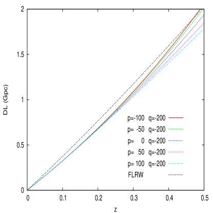
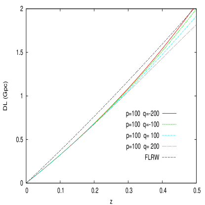
Figure 1: Luminosity distances for a Szekeres model that is not axially or spherically symmetric. To the left, the value of $q$ is fixed to $-200$ while $p$ is varied by taking the values $-100,-50,0,50,100$. To the right, the value of $p$ is fixed to $-100$ while $q$ is varied by taking the values $-200,-100,0,100,200$. The Szekeres inhomogeneous model used here is for an illustration purpose only and was introduced in Bolejko2006a within structure formation context. The model is specified in our section V-A. The luminosity distance for an open FLRW model is plotted as well.

Putting these into equation (40) gives

$$d\ln{D_{A}} = \Big{[}\frac{1}{2}\left(\frac{(F^{2})_{,t}}{F^{2}}k^{t}+\frac{(F^{2})_{,r}}{F^{2}}k^{r}+\frac{(F^{2})_{,p}}{F^{2}}k^{p}+\frac{(F^{2})_{,q}}{F^{2}}k^{q}\right)+$$ (42)

$$\frac{1}{4}\left(\frac{H_{,t}}{H}k^{t}+\frac{H_{,r}}{H}k^{r}+\frac{H_{,p}}{H}k^{p}+\frac{H_{,q}}{H}k^{q}\right)+\frac{1}{2}\left(k^{t}_{,t}+k^{r}_{,r}+k^{p}_{,p}+k^{q}_{,q}\right)\Big{]}ds$$

and upon applying the total derivative equation (22), we get the following equations for the area distance:

$$D_{A}=F\,H^{1/4}\exp{\Big{[}\frac{1}{2}\int^{s}_{s_{0}}{\left(k^{t}_{,t}+k^{r}_{,r}+k^{p}_{,p}+k^{q}_{,q}\right)}d\underline{s}\Big{]}}.$$ (43)

The luminosity distance is given from its relation to the area distance expression (43) as

$$D_{L}=(1+z)^{2}\,D_{A}.$$ (44)

Given explicit functions for a Szekeres model, the area distance is calculated from equation (43) where the components $k^{t}_{,t}$, $k^{r}_{,r}$, $k^{p}_{,p}$, and $k^{q}_{,q}$ are numerically integrated from the system of ODEs derived in section IV and listed in the Appendix. The redshift is also numerically integrated from the null geodesic equations as described in section VI further.

V.1 Examples of luminosity distance versus redshift plots

For illustration, we integrate and plot luminosity distances versus redshift for a Szekeres model that is not axially or spherically symmetric. We use a model that was introduced in Bolejko2006a within large scale structure formation context and we simply use it here for illustration purposes. In this case, we set:

• $\epsilon=+1$.

• $t_{B}(r)=0$ for a simultaneous Big Bang.

• $M(r)=(\sinh(r))^{3}$.

• ${k}(r)=\frac{-1}{1+C^{2}r^{2}}$ (i.e. at large $r$, the spatial curvature goes to zero as indicated by CMB observations observations5 ) and at very small $r$ curvature goes negative in accord with local observations of matter abundances with lower density than the critical density.

• The functions $\{S,P,Q\}$ are given by model-1 of Bolejko2006a with $\{140,10,-113\,ln(1+r)\}$.

The results for various values of $p$ and $q$ values are given in Figure I along with an open FLRW model. The exploration of more sophisticated Szekeres models and comparisons to supernova data and other cosmological distances data will be presented in follow-up investigations.

V.2 Application and verification of special cases

We derived a general expression for the area distance and luminosity distance for the Szekeres models. It is important to verify that these expressions reduce to ones that we know in the special cases.

V.2.1 Axially symmetric case

As explored in Nolan2007 ; BolejkoEtAlBook , the conditions on the Szekeres metric functions for axial symmetry are given by

$$EE_{,pr} = E_{,p}E_{r}$$ (45)

$$EE_{,qr} = E_{,q}E_{r}.$$ (46)

It is trivial to see from our compact notation in the geodesic equations (24) and (25) that these axial symmetry conditions are here simply

$$H_{,p}=H_{,q}=0.$$ (47)

Conditions (47) assure that $dq=dp=0$ holds along the whole geodesic. We proceed then by setting $dp=dq=0$ into equation (26) so $(k^{t})^{2}-H(k^{r})^{2}=0$ or

$$(k^{r})^{2}=\frac{1}{H}(k^{t})^{2}.$$ (48)

Using this in equation (21) and integrating for $(k^{t})^{2}$ gives

$$(k^{t})^{2}=\exp{\left(-\int^{t}_{t_{0}}{\frac{H_{,\underline{t}}}{H}}d\underline{t}\right)}$$ (49)

Now, from (48), we have

$$\frac{dt}{dr}=-\sqrt{H}$$ (50)

and using it in equation (49) and taking its square root gives

$${k^{t}}=\exp{\left(\int^{r}_{r_{0}}{(\sqrt{H}),_{t}}d\underline{r}\right)}$$ (51)

where we have also noted that $\frac{1}{2}\frac{H_{,t}}{\sqrt{H}}=(\sqrt{H})_{,t}$.

Next, using (48), we get immediately for ${k^{r}}$:

$${k^{r}}=-\frac{1}{\sqrt{H}}\exp{\left(\int^{r}_{r_{0}}{(\sqrt{H}),_{t}}d\underline{r}\right)}$$ (52)

These two expressions agree with the ones obtained in BolejkoEtAlBook for the axially symmetric case.

Now, our expression (42) for the area distance reduces to

$$d\ln{D_{A}}=\Big{[}\frac{1}{2}\left(\frac{(F^{2})_{,t}}{F^{2}}k^{t}+\frac{(F^{2})_{,r}}{F^{2}}k^{r}\right)+\frac{1}{4}\left(\frac{H_{,t}}{H}k^{t}+\frac{H_{,r}}{H}k^{r}\right)+\frac{1}{2}\left(k^{t}_{,t}+k^{r}_{,r}\right)\Big{]}ds$$ (53)

where we use the tangent vector component equations (51) and (52) for axial symmetry to express the partial derivatives in the last two terms in (53) as

$$k^{t}_{,t} = \Big{[}-\frac{1}{2}\int^{t}_{t_{0}}{\frac{\left(H_{,\underline{t}}\right)}{H}}d\underline{t}\Big{]}_{,t}k^{t}$$ (54)

$$k^{r}_{,r} = -\frac{1}{2}\frac{H_{,r}}{H}k^{r}+\Big{[}-\frac{1}{2}\int^{t}_{t_{0}}{\frac{\left(H_{,\underline{t}}\right)}{H}}d\underline{t}\Big{]}_{,r}k^{r}.$$ (55)

and where we have used $\frac{dr}{dt}dt=-\frac{1}{\sqrt{H}}dt$ and $\frac{1}{2}\frac{H_{,t}}{\sqrt{H}}=(\sqrt{H})_{,t}$ in equation(55). We also note that with axial symmetry $p$ and $q$ are being constant and we can combine the term in (54) plus the last term in (55) to make a full derivative. Putting this into the integration of the last part of equation (53) gives

$$\frac{1}{2}\int^{s}_{s_{0}}\left(k^{t}_{,t}+k^{r}_{,r}\right)d\underline{s} = -\frac{1}{4}\int^{r}_{r_{0}}\frac{H_{,\underline{r}}}{H}d\underline{r}-\frac{1}{4}\int^{t}_{t_{0}}\frac{H_{,\underline{t}}}{H}d\underline{t}.$$ (56)

These two terms cancel with the integrated two middle terms in equation (53) yielding a straightforward integration result

$$D_{A}=F.$$ (57)

This result is in agreement with the result of BolejkoPrivate ; BolejkoCelerier of the axially symmetric case.

V.2.2 Spherically symmetric case

In the more special case of spherical symmetry, i.e. $\epsilon=+1$ and $E_{,r}=0$, our expression (42) for the area distance reduces to simply

$$d\ln{D_{A}}=\frac{1}{2}\left(\frac{(R^{2})_{,t}}{R^{2}}k^{t}+\frac{(R^{2})_{,r}}{R^{2}}k^{r}\right)ds.$$ (58)

Integrating both sides gives

$$D_{A}=R$$ (59)

which is the well-known result for the observer area distance for an observer located at the center of the Lemaitre-Tolman-Bondi spherical model, see for example PlebanskiAndKrasinski2006 .

VI The redshift in the Szekeres models

In order to plot the luminosity distance as a function of the redshift, the latter needs also to be integrated in all generality. We start with the standard relation

$$1+z=\frac{(k^{\alpha}u_{\alpha})_{e}}{(k^{\alpha}u_{\alpha})_{o}}=\frac{(k^{t})_{e}}{(k^{t})_{o}}$$ (60)

where $k^{\alpha}$ is the affinely parameterized null vector, $u^{\alpha}=(1,0,0,0)$ is the 4-velocity vector, and the subscripts $e$ and $o$ are for emitted (at the source) and observed (at the observer) respectively. Now, we use equation (21) and write

$$\frac{d[(k^{t})^{2}]}{ds}=-(H)_{,t}k^{t}(k^{r})^{2}-\frac{(F^{2})_{,t}}{F^{2}}k^{t}[(k^{t})^{2}-H(k^{r})^{2}]=2k^{t}\frac{dk^{t}}{ds}$$ (61)

which we use along with taking the natural log of both sides of (60) and differentiating both sides wrt to the affine parameter $s$ to obtain

$$\frac{1}{1+z}\frac{dz}{ds}=\frac{1}{k^{t}}\frac{dk^{t}}{ds}=-\frac{1}{2\,k^{t}}\left[(H)_{,t}(k^{r})^{2}+\frac{(F^{2})_{,t}}{F^{2}}((k^{t})^{2}-H(k^{r})^{2})\right].$$ (62)

While it is informative to see this expression, which one can integrate simultaneously with the three other null geodesic equations (23), (24), and (25) to find the redshift, one can equally use equation (60) and get $k^{t}$ by integrating the four null geodesic equations. We proceeded with the latter method for our numerical calculations. An alternative way to find the redshift and the related drift effects in the Szekeres models can be found in KrasinskiandBolejko2011 .

As an aside, we note that using the null condition $k^{\alpha}k_{\alpha}=0$ to substitute $({k}^{t})^{2}-H({k}^{r})^{2}$ by $F^{2}[({k}^{p})^{2}+({k}^{q})^{2}]$, the redshift equation (62) can be written as

$$\frac{1}{1+z}\frac{dz}{ds}=-\frac{1}{2\,k^{t}}\left[(H)_{,t}(k^{r})^{2}+(F^{2})_{,t}((k^{p})^{2}+(k^{q})^{2})\right]$$ (63)

which is precisely the redshift relation that was derived in our previous work IshakEtAl2008 ; FootnoteRedshift .

VI.1 Application and verification of special cases

We derived a general expression for the redshift for the Szekeres models. It is important to verify that this expression reduces to the ones in the known special cases.

VI.1.1 Axially symmetric case

In their recent book BolejkoEtAlBook , the authors derived an expression for the redshift for the axially symmetric Szekeres models that reads:

$$\ln{(1+z)}=\int^{r_{0}}_{r_{e}}{dr\frac{R_{,tr}-R_{,t}\frac{E_{,r}}{E}}{\sqrt{1-k}}}.$$ (64)

Taking the derivative of this equation with respect to the affine parameter, $s$, we get

$$\frac{1}{1+z}\frac{d(1+z)}{ds} = \frac{R_{,tr}-R_{,t}\frac{E_{,r}}{E}}{\sqrt{1-k}}\frac{dr}{ds}$$ (65)

Using our equation for the null condition (26) and $k^{p}=k^{q}=0$ gives

$$\frac{k^{r}}{k^{t}}=-\frac{\sqrt{1-k}}{R_{,r}-R\frac{E_{,r}}{E}}$$ (66)

Now we multiply equation (65) by $\frac{dr/ds}{dr/ds}=\frac{k^{r}}{k^{r}}$ to write

$$\frac{1}{1+z}\frac{d(1+z)}{ds} = \frac{R_{,tr}-R_{,t}\frac{E_{,r}}{E}}{\sqrt{1-k}}\frac{(k^{r})^{2}}{k^{r}}.$$ (67)

We then use equation(66) to substitute for $k^{r}$ in the denominator of equation (67) and expand the numerator to get

$$\frac{1}{1+z}\frac{d(1+z)}{ds}=-\frac{1}{k^{t}}\frac{R_{,tr}R_{,r}+RR_{,t}(\frac{E_{,r}}{E})^{2}-(R_{,r}R_{,t}+RR_{,tr})\frac{E_{,r}}{E}}{1-k}(k^{r})^{2}$$ (68)

Now, we go back to our expression for the redshift, i.e. equation (63) and we put there $k^{p}=k^{q}=0$ as well as the definitions of $H$ and $F$ to re-write it as follows

$$\frac{1}{1+z}\frac{d(1+z)}{ds}=-\frac{1}{k^{t}}\frac{R_{,tr}R_{,r}+RR_{,t}(\frac{E_{,r}}{E})^{2}-(R_{,r}R_{,t}+RR_{,tr})\frac{E_{,r}}{E}}{1-k}(k^{r})^{2}$$ (69)

As one can see our expression for the redshift when reduced to the axially symmetric case agrees with the redshift given in the work of BolejkoEtAlBook for this particular case.

VI.1.2 Spherically symmetric case

The spherically symmetric case happens in the more particular case where $E_{,r}=0$. Substituting this condition into equation (69) gives

$$\frac{1}{1+z}\frac{d(1+z)}{ds}=-\frac{1}{k^{t}}\frac{R_{,tr}R_{,r}}{1-k}(k^{r})^{2}.$$ (70)

Using equation (66) into equation (70) gives

$$\frac{1}{1+z}\frac{d(1+z)}{ds}=\frac{R_{,tr}}{\sqrt{1-k}}k^{r}$$ (71)

that upon integration yields

$$\ln{(1+z)}=\int^{r_{0}}_{r_{e}}{dr\frac{R_{,tr}}{\sqrt{1-k}}}$$ (72)

which is the usual result for the spherically symmetric Lemaitre-Tolman-Bondi models, see for example PlebanskiAndKrasinski2006 .

VII Conclusion

We derived and used a framework to integrate the area and luminosity distances in the general Szekeres models. We used the general affinely parameterized null geodesic equations in order to derive a set of first-order ordinary differential equations that can be integrated numerically to calculate the partial derivatives of the null vector components. These equations allow the numerical integration of the area and luminosity distances in the general Szekeres models. We determined the redshift from simultaneous integration of the null geodesic equations. This work does not assume spherical or axial symmetry and will be useful for comparisons of the general Szekeres inhomogeneous models to current and future cosmological data.

Appendix A Set of ODEs for the partial derivatives of the null vector components

Equation (31) from section IV expands into the following 4 ODEs:

$$H\left[\frac{d}{ds}(k^{r}_{,t})+k^{r}_{,t}k^{t}_{,t}+k^{r}_{,r}k^{r}_{,t}+k^{r}_{,p}k^{p}_{,t}+k^{r}_{,q}k^{q}_{,t}\right]+H_{,t}\frac{d}{ds}(k^{r})$$

$$+\left[H_{,tt}k^{t}+H_{,rt}k^{r}+H_{,pt}k^{p}+H_{,qt}k^{q}+H_{,t}k^{t}_{,t}+H_{,r}k^{r}_{,t}+H_{,p}k^{p}_{,t}+H_{,q}k^{q}_{,t}\right]k^{r}+$$

$$H_{,t}k^{t}k^{r}_{,t}+H_{,r}k^{r}k^{r}_{,t}+H_{,p}k^{p}k^{r}_{,t}+H_{,q}k^{q}k^{r}_{,t}-\frac{1}{2}H_{,rt}(k^{r})^{2}-H_{,r}k^{r}k^{r}_{,t}$$

$$-\frac{1}{2}\left(\frac{(F^{2})_{,r}}{F^{2}}\right)_{,t}\left((k^{t})^{2}-H(k^{r})^{2}\right)-\frac{(F^{2})_{,r}}{F^{2}}\left(k^{t}k^{t}_{,t}-\frac{1}{2}H_{,t}(k^{r})^{2}-Hk^{r}k^{r}_{,t}\right)=0$$ (73)

$$H\left[\frac{d}{ds}(k^{r}_{,r})+k^{r}_{,t}k^{t}_{,r}+k^{r}_{,r}k^{r}_{,r}+k^{r}_{,p}k^{p}_{,r}+k^{r}_{,q}k^{q}_{,r}\right]+H_{,r}\frac{d}{ds}(k^{r})$$

$$+\left[H_{,tr}k^{t}+H_{,rr}k^{r}+H_{,pr}k^{p}+H_{,qr}k^{q}+H_{,t}k^{t}_{,r}+H_{,r}k^{r}_{,r}+H_{,p}k^{p}_{,r}+H_{,q}k^{q}_{,r}\right]k^{r}+$$

$$H_{,t}k^{t}k^{r}_{,r}+H_{,r}k^{r}k^{r}_{,r}+H_{,p}k^{p}k^{r}_{,r}+H_{,q}k^{q}k^{r}_{,r}-\frac{1}{2}H_{,rr}(k^{r})^{2}-H_{,r}k^{r}k^{r}_{,r}$$

$$-\frac{1}{2}\left(\frac{(F^{2})_{,r}}{F^{2}}\right)_{,r}\left((k^{t})^{2}-H(k^{r})^{2}\right)-\frac{(F^{2})_{,r}}{F^{2}}\left(k^{t}k^{t}_{,r}-\frac{1}{2}H_{,r}(k^{r})^{2}-Hk^{r}k^{r}_{,r}\right)=0$$ (74)

$$H\left[\frac{d}{ds}(k^{r}_{,p})+k^{r}_{,t}k^{t}_{,p}+k^{r}_{,r}k^{r}_{,p}+k^{r}_{,p}k^{p}_{,p}+k^{r}_{,q}k^{q}_{,p}\right]+H_{,p}\frac{d}{ds}(k^{r})$$

$$+\left[H_{,tp}k^{t}+H_{,rp}k^{r}+H_{,pp}k^{p}+H_{,qp}k^{q}+H_{,t}k^{t}_{,p}+H_{,r}k^{r}_{,p}+H_{,p}k^{p}_{,p}+H_{,q}k^{q}_{,p}\right]k^{r}+$$

$$H_{,t}k^{t}k^{r}_{,p}+H_{,r}k^{r}k^{r}_{,p}+H_{,p}k^{p}k^{r}_{,p}+H_{,q}k^{q}k^{r}_{,p}-\frac{1}{2}H_{,rp}(k^{r})^{2}-H_{,r}k^{r}k^{r}_{,p}$$

$$-\frac{1}{2}\left(\frac{(F^{2})_{,r}}{F^{2}}\right)_{,p}\left((k^{t})^{2}-H(k^{r})^{2}\right)-\frac{(F^{2})_{,r}}{F^{2}}\left(k^{t}k^{t}_{,p}-\frac{1}{2}H_{,p}(k^{r})^{2}-Hk^{r}k^{r}_{,p}\right)=0$$ (75)

$$H\left[\frac{d}{ds}(k^{r}_{,q})+k^{r}_{,t}k^{t}_{,q}+k^{r}_{,r}k^{r}_{,q}+k^{r}_{,p}k^{p}_{,q}+k^{r}_{,q}k^{q}_{,q}\right]+H_{,q}\frac{d}{ds}(k^{r})$$

$$+\left[H_{,tq}k^{t}+H_{,rq}k^{r}+H_{,pq}k^{p}+H_{,qq}k^{q}+H_{,t}k^{t}_{,q}+H_{,r}k^{r}_{,q}+H_{,p}k^{p}_{,q}+H_{,q}k^{q}_{,q}\right]k^{r}+$$

$$H_{,t}k^{t}k^{r}_{,q}+H_{,r}k^{r}k^{r}_{,q}+H_{,p}k^{p}k^{r}_{,q}+H_{,q}k^{q}k^{r}_{,q}-\frac{1}{2}H_{,rq}(k^{r})^{2}-H_{,r}k^{r}k^{r}_{,q}$$

$$-\frac{1}{2}\left(\frac{(F^{2})_{,r}}{F^{2}}\right)_{,q}\left((k^{t})^{2}-H(k^{r})^{2}\right)-\frac{(F^{2})_{,r}}{F^{2}}\left(k^{t}k^{t}_{,q}-\frac{1}{2}H_{,q}(k^{r})^{2}-Hk^{r}k^{r}_{,q}\right)=0$$ (76)

where $\frac{d}{ds}(k^{r})$ is written in terms of metric functions and null vector components from equation (27) (i.e. (32)).

Equation (33) from section IV expands into the following 4 ODEs:

$$\frac{d}{ds}(k^{t}_{,t})+k^{t}_{,t}k^{t}_{,t}+k^{t}_{,r}k^{r}_{,t}+k^{t}_{,p}k^{p}_{,t}+k^{t}_{,q}k^{q}_{,t}+\frac{1}{2}H_{,tt}(k^{r})^{2}+H_{,t}k^{r}k^{r}_{,t}+\frac{1}{2}\left(\frac{(F^{2})_{,t}}{F^{2}}\right)_{,t}\left((k^{t})^{2}-H(k^{r})^{2}\right)$$

$$+\frac{(F^{2})_{,t}}{F^{2}}\left(k^{t}k^{t}_{,t}-\frac{1}{2}H_{,t}(k^{r})^{2}-Hk^{r}k^{r}_{,t}\right)=0$$ (77)

$$\frac{d}{ds}(k^{t}_{,r})+k^{t}_{,t}k^{t}_{,r}+k^{t}_{,r}k^{r}_{,r}+k^{t}_{,p}k^{p}_{,r}+k^{t}_{,q}k^{q}_{,r}+\frac{1}{2}H_{,tr}(k^{r})^{2}+H_{,t}k^{r}k^{r}_{,r}+\frac{1}{2}\left(\frac{(F^{2})_{,t}}{F^{2}}\right)_{,r}\left((k^{t})^{2}-H(k^{r})^{2}\right)$$

$$+\frac{(F^{2})_{,t}}{F^{2}}\left(k^{t}k^{t}_{,r}-\frac{1}{2}H_{,r}(k^{r})^{2}-Hk^{r}k^{r}_{,r}\right)=0$$ (78)

$$\frac{d}{ds}(k^{t}_{,p})+k^{t}_{,t}k^{t}_{,p}+k^{t}_{,r}k^{r}_{,p}+k^{t}_{,p}k^{p}_{,p}+k^{t}_{,q}k^{q}_{,p}+\frac{1}{2}H_{,tp}(k^{r})^{2}+H_{,t}k^{r}k^{r}_{,p}+\frac{1}{2}\left(\frac{(F^{2})_{,t}}{F^{2}}\right)_{,p}\left((k^{t})^{2}-H(k^{r})^{2}\right)$$

$$+\frac{(F^{2})_{,t}}{F^{2}}\left(k^{t}k^{t}_{,p}-\frac{1}{2}H_{,p}(k^{r})^{2}-Hk^{r}k^{r}_{,p}\right)=0$$ (79)

$$\frac{d}{ds}(k^{t}_{,q})+k^{t}_{,t}k^{t}_{,q}+k^{t}_{,r}k^{r}_{,q}+k^{t}_{,p}k^{p}_{,q}+k^{t}_{,q}k^{q}_{,q}+\frac{1}{2}H_{,tq}(k^{r})^{2}+H_{,t}k^{r}k^{r}_{,q}+\frac{1}{2}\left(\frac{(F^{2})_{,t}}{F^{2}}\right)_{,q}\left((k^{t})^{2}-H(k^{r})^{2}\right)$$

$$+\frac{(F^{2})_{,t}}{F^{2}}\left(k^{t}k^{t}_{,q}-\frac{1}{2}H_{,q}(k^{r})^{2}-Hk^{r}k^{r}_{,q}\right)=0.$$ (80)

Equation (34) from section IV expands into the following 4 ODEs:

$$F^{2}\left[\frac{d}{ds}(k^{p}_{,t})+k^{p}_{,t}k^{t}_{,t}+k^{p}_{,r}k^{r}_{,t}+k^{p}_{,p}k^{p}_{,t}+k^{p}_{,q}k^{q}_{,t}\right]+(F^{2})_{,t}\frac{d}{ds}(k^{p})-\frac{1}{2}H_{,pt}(k^{r})^{2}-H_{,p}k^{r}k^{r}_{,t}+$$

$$\left[(F^{2})_{,tt}k^{t}+(F^{2})_{,rt}k^{r}+(F^{2})_{,pt}k^{p}+(F^{2})_{,qt}k^{q}+(F^{2})_{,t}k^{t}_{,t}+(F^{2})_{,r}k^{r}_{,t}+(F^{2})_{,p}k^{p}_{,t}+(F^{2})_{,q}k^{q}_{,t}\right]k^{p}+$$

$$\left((F^{2})_{,t}k^{t}+(F^{2})_{,r}k^{r}+(F^{2})_{,p}k^{p}+(F^{2})_{,q}k^{q}\right)k^{p}_{,t}-\frac{1}{2}\left(\frac{(F^{2})_{,p}}{F^{2}}\right)_{,t}\left((k^{t})^{2}-H(k^{r})^{2}\right)$$

$$-\frac{(F^{2})_{,p}}{F^{2}}\left(k^{t}k^{t}_{,t}-\frac{1}{2}H_{,t}(k^{r})^{2}-Hk^{r}k^{r}_{,t}\right)=0$$ (81)

$$F^{2}\left[\frac{d}{ds}(k^{p}_{,r})+k^{p}_{,t}k^{t}_{,r}+k^{p}_{,r}k^{r}_{,r}+k^{p}_{,p}k^{p}_{,r}+k^{p}_{,q}k^{q}_{,r}\right]+(F^{2})_{,r}\frac{d}{ds}(k^{p})-\frac{1}{2}H_{,pr}(k^{r})^{2}-H_{,p}k^{r}k^{r}_{,r}+$$

$$\left[(F^{2})_{,tr}k^{t}+(F^{2})_{,rr}k^{r}+(F^{2})_{,pr}k^{p}+(F^{2})_{,qr}k^{q}+(F^{2})_{,t}k^{t}_{,r}+(F^{2})_{,r}k^{r}_{,r}+(F^{2})_{,p}k^{p}_{,r}+(F^{2})_{,q}k^{q}_{,r}\right]k^{p}+$$

$$\left((F^{2})_{,t}k^{t}+(F^{2})_{,r}k^{r}+(F^{2})_{,p}k^{p}+(F^{2})_{,q}k^{q}\right)k^{p}_{,r}-\frac{1}{2}\left(\frac{(F^{2})_{,p}}{F^{2}}\right)_{,r}\left((k^{t})^{2}-H(k^{r})^{2}\right)$$

$$-\frac{(F^{2})_{,p}}{F^{2}}\left(k^{t}k^{t}_{,r}-\frac{1}{2}H_{,r}(k^{r})^{2}-Hk^{r}k^{r}_{,r}\right)=0$$ (82)

$$F^{2}\left[\frac{d}{ds}(k^{p}_{,p})+k^{p}_{,t}k^{t}_{,p}+k^{p}_{,r}k^{r}_{,p}+k^{p}_{,p}k^{p}_{,p}+k^{p}_{,q}k^{q}_{,p}\right]+(F^{2})_{,p}\frac{d}{ds}(k^{p})-\frac{1}{2}H_{,pp}(k^{r})^{2}-H_{,p}k^{r}k^{r}_{,p}+$$

$$\left[(F^{2})_{,tp}k^{t}+(F^{2})_{,rp}k^{r}+(F^{2})_{,pp}k^{p}+(F^{2})_{,qp}k^{q}+(F^{2})_{,t}k^{t}_{,p}+(F^{2})_{,r}k^{r}_{,p}+(F^{2})_{,p}k^{p}_{,p}+(F^{2})_{,q}k^{q}_{,p}\right]k^{p}+$$

$$\left((F^{2})_{,t}k^{t}+(F^{2})_{,r}k^{r}+(F^{2})_{,p}k^{p}+(F^{2})_{,q}k^{q}\right)k^{p}_{,p}-\frac{1}{2}\left(\frac{(F^{2})_{,p}}{F^{2}}\right)_{,p}\left((k^{t})^{2}-H(k^{r})^{2}\right)$$

$$-\frac{(F^{2})_{,p}}{F^{2}}\left(k^{t}k^{t}_{,p}-\frac{1}{2}H_{,p}(k^{r})^{2}-Hk^{r}k^{r}_{,p}\right)=0$$ (83)

$$F^{2}\left[\frac{d}{ds}(k^{p}_{,q})+k^{p}_{,t}k^{t}_{,q}+k^{p}_{,r}k^{r}_{,q}+k^{p}_{,p}k^{p}_{,q}+k^{p}_{,q}k^{q}_{,q}\right]+(F^{2})_{,q}\frac{d}{ds}(k^{p})-\frac{1}{2}H_{,pq}(k^{r})^{2}-H_{,p}k^{r}k^{r}_{,q}+$$

$$\left[(F^{2})_{,tq}k^{t}+(F^{2})_{,rq}k^{r}+(F^{2})_{,pq}k^{p}+(F^{2})_{,qq}k^{q}+(F^{2})_{,t}k^{t}_{,q}+(F^{2})_{,r}k^{r}_{,q}+(F^{2})_{,p}k^{,p}_{q}+(F^{2})_{,q}k^{q}_{,q}\right]k^{p}+$$

$$\left((F^{2})_{,t}k^{t}+(F^{2})_{,r}k^{r}+(F^{2})_{,p}k^{p}+(F^{2})_{,q}k^{q}\right)k^{p}_{,q}-\frac{1}{2}\left(\frac{(F^{2})_{,p}}{F^{2}}\right)_{,q}\left((k^{t})^{2}-H(k^{r})^{2}\right)$$

$$-\frac{(F^{2})_{,p}}{F^{2}}\left(k^{t}k^{t}_{,q}-\frac{1}{2}H_{,q}(k^{r})^{2}-Hk^{r}k^{r}_{,q}\right)=0$$ (84)

where $\frac{d}{ds}(k^{p})$ is written in terms of the metric functions and the null vector components from equation (24).

Equation (35) from section IV expands into the following 4 ODEs:

$$F^{2}\left[\frac{d}{ds}(k^{q}_{,t})+k^{q}_{,t}k^{t}_{,t}+k^{q}_{,r}k^{r}_{,t}+k^{q}_{,p}k^{p}_{,t}+k^{q}_{,q}k^{q}_{,t}\right]+(F^{2})_{,t}\frac{d}{ds}(k^{q})-\frac{1}{2}H_{,qt}(k^{r})^{2}-H_{,q}k^{r}k^{r}_{,t}+$$

$$\left[(F^{2})_{,tt}k^{t}+(F^{2})_{,rt}k^{r}+(F^{2})_{,pt}k^{p}+(F^{2})_{,qt}k^{q}+(F^{2})_{,t}k^{t}_{,t}+(F^{2})_{,r}k^{r}_{,t}+(F^{2})_{,p}k^{p}_{,t}+(F^{2})_{,q}k^{q}_{,t}\right]k^{q}+$$

$$\left((F^{2})_{,t}k^{t}+(F^{2})_{,r}k^{r}+(F^{2})_{,p}k^{p}+(F^{2})_{,q}k^{q}\right)k^{q}_{,t}-\frac{1}{2}\left(\frac{(F^{2})_{,q}}{F^{2}}\right)_{,t}\left((k^{t})^{2}-H(k^{r})^{2}\right)$$

$$-\frac{(F^{2})_{,q}}{F^{2}}\left(k^{t}k^{t}_{,t}-\frac{1}{2}H_{,t}(k^{r})^{2}-Hk^{r}k^{r}_{,t}\right)=0$$ (85)

$$F^{2}\left[\frac{d}{ds}(k^{q}_{,r})+k^{q}_{,t}k^{t}_{,r}+k^{q}_{,r}k^{r}_{,r}+k^{q}_{,p}k^{p}_{,r}+k^{q}_{,q}k^{q}_{,r}\right]+(F^{2})_{,r}\frac{d}{ds}(k^{q})-\frac{1}{2}H_{,qr}(k^{r})^{2}-H_{,q}k^{r}k^{r}_{,r}+$$

$$\left[(F^{2})_{,tr}k^{t}+(F^{2})_{,rr}k^{r}+(F^{2})_{,pr}k^{p}+(F^{2})_{,qr}k^{q}+(F^{2})_{,t}k^{t}_{,r}+(F^{2})_{,r}k^{r}_{,r}+(F^{2})_{,p}k^{p}_{,r}+(F^{2})_{,q}k^{q}_{,r}\right]k^{q}+$$

$$\left((F^{2})_{,t}k^{t}+(F^{2})_{,r}k^{r}+(F^{2})_{,p}k^{p}+(F^{2})_{,q}k^{q}\right)k^{q}_{,r}-\frac{1}{2}\left(\frac{(F^{2})_{,q}}{F^{2}}\right)_{,r}\left((k^{t})^{2}-H(k^{r})^{2}\right)$$

$$-\frac{(F^{2})_{,q}}{F^{2}}\left(k^{t}k^{t}_{,r}-\frac{1}{2}H_{,r}(k^{r})^{2}-Hk^{r}k^{r}_{,r}\right)=0$$ (86)

$$F^{2}\left[\frac{d}{ds}(k^{q}_{,p})+k^{q}_{,t}k^{t}_{,p}+k^{q}_{,r}k^{r}_{,p}+k^{q}_{,p}k^{p}_{,p}+k^{q}_{,q}k^{q}_{,p}\right]+(F^{2})_{,p}\frac{d}{ds}(k^{q})-\frac{1}{2}H_{,qp}(k^{r})^{2}-H_{,q}k^{r}k^{r}_{,p}+$$

$$\left[(F^{2})_{,tp}k^{t}+(F^{2})_{,rp}k^{r}+(F^{2})_{,pp}k^{p}+(F^{2})_{,qp}k^{q}+(F^{2})_{,t}k^{t}_{,p}+(F^{2})_{,r}k^{r}_{,p}+(F^{2})_{,p}k^{p}_{,p}+(F^{2})_{,q}k^{q}_{,p}\right]k^{q}+$$

$$\left((F^{2})_{,t}k^{t}+(F^{2})_{,r}k^{r}+(F^{2})_{,p}k^{p}+(F^{2})_{,q}k^{q}\right)k^{q}_{,p}-\frac{1}{2}\left(\frac{(F^{2})_{,q}}{F^{2}}\right)_{,p}\left((k^{t})^{2}-H(k^{r})^{2}\right)$$

$$-\frac{(F^{2})_{,q}}{F^{2}}\left(k^{t}k^{t}_{,p}-\frac{1}{2}H_{,p}(k^{r})^{2}-Hk^{r}k^{r}_{,p}\right)=0$$ (87)

$$F^{2}\left[\frac{d}{ds}(k^{q}_{,q})+k^{q}_{,t}k^{t}_{,q}+k^{q}_{,r}k^{r}_{,q}+k^{q}_{,p}k^{p}_{,q}+k^{q}_{,q}k^{q}_{,q}\right]+(F^{2})_{,q}\frac{d}{ds}(k^{q})-\frac{1}{2}H_{,qq}(k^{r})^{2}-H_{,q}k^{r}k^{r}_{,q}+$$

$$\left[(F^{2})_{,tq}k^{t}+(F^{2})_{,rq}k^{r}+(F^{2})_{,pq}k^{p}+(F^{2})_{,qq}k^{q}+(F^{2})_{,t}k^{t}_{,q}+(F^{2})_{,r}k^{r}_{,q}+(F^{2})_{,p}k^{p}_{,q}+(F^{2})_{,q}k^{q}_{,q}\right]k^{q}+$$

$$\left((F^{2})_{,t}k^{t}+(F^{2})_{,r}k^{r}+(F^{2})_{,p}k^{p}+(F^{2})_{,q}k^{q}\right)k^{q}_{,q}-\frac{1}{2}\left(\frac{(F^{2})_{,q}}{F^{2}}\right)_{,q}\left((k^{t})^{2}-H(k^{r})^{2}\right)$$

$$-\frac{(F^{2})_{,q}}{F^{2}}\left(k^{t}k^{t}_{,q}-\frac{1}{2}H_{,q}(k^{r})^{2}-Hk^{r}k^{r}_{,q}\right)=0.$$ (88)

where $\frac{d}{ds}(k^{q})$ is written in terms of the metric functions and the null vector components from equation (25).

Finally, equation (36) from section IV expands into the following 4 equations:

$$k^{r}_{,t}=\frac{1}{2k^{r}}\left[-\frac{H_{,t}}{H}(k^{r})^{2}+\frac{1}{H}\left(2k^{t}k^{t}_{,t}-(F^{2})_{,t}\left((k^{p})^{2}+(k^{q})^{2}\right)-2F^{2}\left(k^{p}k^{p}_{,t}+k^{q}k^{q}_{,t}\right)\right)\right]$$ (89)

$$k^{r}_{,r}=\frac{1}{2k^{r}}\left[-\frac{H_{,r}}{H}(k^{r})^{2}+\frac{1}{H}\left(2k^{t}k^{t}_{,r}-(F^{2})_{,r}\left((k^{p})^{2}+(k^{q})^{2}\right)-2F^{2}\left(k^{p}k^{p}_{,r}+k^{q}k^{q}_{,r}\right)\right)\right]$$ (90)

$$k^{r}_{,p}=\frac{1}{2k^{r}}\left[-\frac{H_{,p}}{H}(k^{r})^{2}+\frac{1}{H}\left(2k^{t}k^{t}_{,p}-(F^{2})_{,p}\left((k^{p})^{2}+(k^{q})^{2}\right)-2F^{2}\left(k^{p}k^{p}_{,p}+k^{q}k^{q}_{,p}\right)\right)\right]$$ (91)

$$k^{r}_{,q}=\frac{1}{2k^{r}}\left[-\frac{H_{,q}}{H}(k^{r})^{2}+\frac{1}{H}\left(2k^{t}k^{t}_{,q}-(F^{2})_{,q}\left((k^{p})^{2}+(k^{q})^{2}\right)-2F^{2}\left(k^{p}k^{p}_{,q}+k^{q}k^{q}_{,q}\right)\right)\right]$$ (92)

References

(1) M-N. Celerier, New Advances in Physics 1, 29 (2007). astro-ph/0702416.
(2) K Bolejko, A Krasinski, C Hellaby and MN Celerier,
Structures in the Universe by Exact Methods: Formation, Evolution, Interactions
(Cambridge University Press, 2009).
(3) A. Krasinski, C. Hellaby, Phys. Rev. D 65, 023501 (2002).
(4) C. Hellaby, A. Krasinski, Phys. Rev. D 73, 023518 (2006).
(5) K. Bolejko, Phys. Rev. D 73, 123508 (2006).
(6) K. Bolejko, Phys. Rev. D 75, 043508 (2007).
(7)
H. Iguchi, T. Nakamura and K. i. Nakao, Prog. Theor. Phys. 108, 809 (2002).
(8)
H. Alnes, M. Amarzguioui, O. Gron
Phys. Rev. D73, 083519 (2006).
(9) K. Enqvist, Gen. Rel. Grav. 40:451-466 (2008).
(10)
D. Garfinkle, Class. Quant. Grav. 23, 4811 (2006).
(11)
T. Kai, H. Kozaki, K. Nakao, Y. Nambu, C Yoo
Prog. Theor. Phys. 117, 229 (2007).
(12)
T. Biswas, R. Mansouri, A. Notari,
Journal of Cosmology and Astroparticle Physics 12:017 (2007).
(13)
N. Tanimoto and Y Nambu,
Class. Quantum Grav. 24, 3843 (2007).
(14)
P. Hunt, S. Sarkar, Mon. Not. R. Astron. Soc. 401 (2010) 547.
(15) K. Enqvist, T. Mattsson, JCAP 0702:019 (2007).
(16)
M. Ishak, J. Richardson, D. Garred, D. Whittington, A. Nwankwo, R. Sussman,
Phys. Rev. D 78, 123531 (2008)
(17) D. Chung, A. Romano, Phys. Rev. D 74:103507 (2006).
(18) J. Garcia-Bellido, T. Haugboelle, JCAP 0804:003 (2008).
(19) K. Bolejko and M-N. Celerier, arXiv:1005.2584 (2010).
(21)H. Stephani, D. Kramer, M. MacCallum, C. Hoenselaers and E. Herlt Exact Solutions of Einstein’s Field Equations (Cambridge University Press, Cambridge, 2003).
(22) P. Szekeres, Communications in Mathematical Physics 41, 55 (1975).
(23) P. Szekeres, Phys. Rev. D. 12, 10 (1975).
(24) J. Plebanski and A. Krasinski, An Introduction to General Relativity and Cosmology, (Cambridge, 2006).
(25) D. Szafron, J. Math. Phys. 18, 1673 (1977).
(26) W. Bonnor and N. Tomimura, Mon. Not. R. Astron. Soc. 175, 85 (1976).
(27) W. Bonnor, A. H. Sulaiman, and N. Tomimura, Gen. Relativ. Gravit. 8, 549 (1977).
(28) S. Goode and J. Wainwright, Phys. Rev. D. 26 12 (1982)
(29) W. Bonnor, Classical and Quantum Gravity 3, 495 (1986).
(30) J. Barrow and J. Stein-Chabes, Phys. Letters 103A, 315 (1984).
(31) R. Sussman, J. Triginer, Classical and Quantum Gravity 16, 167 (1999.
(32) C. Hellaby, A. Krasinski, Phys. Rev. D66, 084011 (2002).
(33) C Hellaby and A. Krasinski, Phys. Rev. D 77:023529, (2008).
(34) A. Krasinski, Phys. Rev. D 78, 064038 (2008).
(35) G.F.R. Ellis and H. Van Ellst H.
Cosmological Models. Carguese Lectures 1998. Proceedings of the NATO Advanced Study Institute on Theoretical and Observational Cosmology, Cargese, France, August 17-29, 1998 / edited by Marc Lachieze-Rey. Boston : Kluwer Academic, 1999. NATO science series. Series C, vol. 541, p.1-116
(36) K. Bolejko, Gen. Rel. Grav. 41:1737-1755 (2009).
(37) B. Nolan, U. Debnath, Phys. Rev. D 76, 104046 (2007).
(38) We note that in our previous work, IshakEtAl2008 , some mere sign typos appeared in equation (16) during the late stage of editing the manuscript. Similarly, in equations (32) and (33) there should be a tilde on the . The limits of validity of equation (32) in IshakEtAl2008 will be addressed elsewhere by the authors.
(39) Press et al., Numerical Recipes in C, Cambridge University Press (1992);
(40) P. Sachs, Proc. R. Soc. London A 264, 309 (1961).
(41) R. Kantowski, Astrophys. Journal 155, 89 (1969).
(42)
C. L. Bennett et al.,
Astrophys. J. Suppl. Ser. 148, 1 (2003);
D. N. Spergel et al.,
Astrophys. J. Suppl. Ser. , 175 (2003);
L. Page et al.,
Astrophys. J. Suppl. Ser. 148, 2333 (2003).
E. Komatsu et al., (2010), arXiv:1001.4538.
(43) A. Krasinski, K. Bolejko Phys. Rev. D 83, 083503 (2011).
(44) Substitute and by their simple expressions in order to get equation (26) of IshakEtAl2008 . Note that a prime is missing in equation (22), (25), and (26) on the first occurrence of in the numerator. It is worth noting that equation (26) for the redshift in IshakEtAl2008 is verified here to be correct. Its simultaneous integration with the null geodesic equations provides the redshift in all generality. However, it is unclear at this moment what are the precise limitations of the step between (18) and (19) in IshakEtAl2008 .
(45) K. Bolejko, private communication (2009) and see also BolejkoCelerier .