Green’s Functions and the Adiabatic Hyperspherical Method

Abstract

We address the few-body problem using the adiabatic hyperspherical representation. A general form for the hyperangular Green’s function in $d$-dimensions is derived. The resulting Lippmann-Schwinger equation is solved for the case of three-particles with s-wave zero-range interactions. Identical particle symmetry is incorporated in a general and intuitive way. Complete semi-analytic expressions for the nonadiabatic channel couplings are derived. Finally, a model to describe the atom-loss due to three-body recombination for a three-component fermi-gas of ⁶Li atoms is presented.

I Introduction

In recent years, there has been extensive theoretical and experimental interest in the area of few-body physics, most notably in the famous effect first predicted in 1970 by Vitaly Efimov efimov1971wbs . Efimov studied a three boson system with short-range two-body interactions in which each two-body system is infinitesimally close to forming a bound state; that is, the s-wave scattering length is infinite, or at least very large in magnitude. Quantitatively, Efimov and later others, found that this effect is described by a simple wave function in the hyperspherical representation efimov1973 ; macek1986lbs ; esry1999rta ; nielsen1999ler . A quantitative understanding of three-body scattering esry1999rta ; braaten2004edr has given experiments the tools to examine three-body processes in dilute gas systems and has led to a wealth of experimental evidence for the Efimov effect kraemer2006eeq ; zaccanti2009oes ; ottenstein2008cst ; huckans2009tbr ; gross2009ouu ; pollack2009utf . More recently, predictions relating to the four-body loss rate vonstecher2009suf have given another handle on characterizing an Efimov resonance. The experimental realization of these predictions swiftly followed ferlaino2009euf ; pollack2009utf .

The sticking point of the adiabatic hyperspherical method lies in solving the adiabatic Schrödinger equation. Often solving this $(d-1)$-dimensional equation is as hard as solving the total $d$-dimensional Schrödinger equation in the first place. Having a variety of methods available is therefore helpful. The benefit of using the adiabatic hyperspherical method comes from the simple final interpretation that can often be applied to the resulting coupled set of one-dimensional equations in the hyperradiusfano1981utc . For instance, in the three-body problem, if two particles can form a bound state, then one of the resulting scattering channels consists of an atom and a dimer colliding. In the adiabatic hyperspherical method this type of fragmentation channel arises naturally as one of the discrete solutions to the hyperangular equations. In this paper, we derive the hyperangular Green’s function for an arbitrary $d$-dimensional system, which can then be used in a hyperangular Lippmann-Schwinger equation to extract the adiabatic hyperradial potential curves.

This article is arranged as follows, in Section II we derive a general form of the hyperangular Green’s function for a $d$-dimensional system. In Section III the Green’s function is applied to the problem of three particles with regularized, zero-range, s-wave interactions. Section IV applies this result to the three lowest hyperfine states of ⁶Li, and gives a simple description of the scaling behavior of three-body recombination events that result in trap losses. Finally, in Section V we summarize the results and suggest further avenues of inquiry.

II The hyperangular Green’s function

The adiabatic hyperspherical method has proven useful for analyzing many few-body systems fano1976dee ; clark1980hat ; Avery ; zhou1993hac ; lin1995hca ; kokoouline2003utt . The heart of this method lies in treating the overall size of the system, the hyperradius $R$ defined by $\sqrt{\mu}R=\sqrt{\sum_{i=1}^{d}\mu_{i}x_{i}^{2}}$, as an adiabatic parameter. Here $\mu_{i}$ is the mass scale associated with the $i$th cartesian coordinate and $\mu$ is the reduced mass associated with the hyperradius. For a system of $N$ particles, $x_{i}$ denote the $d=3N-3$ cartesian components needed to specify the relative positions of the $N$ paticles. In this representation, the total wavefunction is written:

$$\Psi\left(R,\Omega\right)=\sum_{n}R^{-\left(d-1\right)/2}F_{n}\left(R\right)\Phi_{n}\left(R;\Omega\right),$$ (1)

where the adiabatic eigenfunctions $\Phi_{n}(R;\Omega)$ satisfy the fixed-$R$ Schrödinger equation:

$$\left[\dfrac{\hbar^{2}}{2\mu}\dfrac{\Lambda^{2}}{R^{2}}+V\left(R,\Omega\right)\right]\Phi_{n}\left(R;\Omega\right)=u_{n}\left(R\right)\Phi_{n}\left(R;\Omega\right),$$ (2)

Here, $\Lambda$ is the grand angular momentum operator defined by

$$\Lambda^{2} =-\sum_{i<j}\Lambda_{ij}^{2}$$ (3)

$$\Lambda_{ij} =x_{i}\dfrac{\partial}{\partial x_{j}}-x_{j}\dfrac{\partial}{\partial x_{i}}.$$ (4)

Inserting Eq. (1) into the full (time-independent) Schrödinger equation takes a $d$-dimensional partial differential equation to a set of coupled one-dimensional differential equations:

$$\left[-\dfrac{\hbar^{2}}{2\mu}\left(\dfrac{d^{2}}{dR^{2}}-\dfrac{\left(d-3\right)\left(d-1\right)}{4R^{2}}\right)+u_{n}\left(R\right)\right]F_{n}\left(R\right)$$

$$-\dfrac{\hbar^{2}}{2\mu}\sum_{m}\left[2P_{nm}\dfrac{d}{dR}+Q_{nm}\right]F_{m}\left(R\right)=EF_{n}\left(R\right)$$ (5)

The non-adiabatic coupling matrices $P$ and $Q$ in Eq. (2) are defined as

$$P_{mn} =\left\langle\Phi_{m}\left(R;\Omega\right){\Huge|}\dfrac{\partial}{\partial R}\Phi_{n}\left(R;\Omega\right)\right\rangle,$$ (6)

$$Q_{mn} =\left\langle\Phi_{m}\left(R;\Omega\right){\Huge|}\dfrac{\partial^{2}}{\partial R^{2}}\Phi_{n}\left(R;\Omega\right)\right\rangle.$$ (7)

The integrals in Eqs. (6) and (7) are taken only over the $d-1$ hyperangles collectively denoted $\Omega$.

Approximate solutions can be found by solving the uncoupled system of equations, which are referred to as the adiabatic approximation:

$$\left[-\dfrac{\hbar^{2}}{2\mu}\dfrac{d^{2}}{dR^{2}}+\dfrac{\hbar^{2}}{2\mu}\dfrac{\left(d-3\right)\left(d-1\right)}{4R^{2}}\right.$$

$$-\left.\dfrac{\hbar^{2}}{2\mu}Q_{nn}+u_{n}\left(R\right)\right]F_{n}\left(R\right)=EF_{n}\left(R\right)$$ (8)

The ground state eigenenergy Eq. (8) is a variational upper bound to the exact ground state energy from Eq. (5). Another variant of this method is frequently denoted the Born-Oppenheimer approximation, with the diagonal correction $-\dfrac{\hbar^{2}}{2\mu}Q_{nn}(R)$ to the potential $u_{n}(R)$ omitted. These two approximations will be the main focus of this paper, while the non-adiabatic couplings $P_{nm}(R)$ will be used to describe Landau-Zener-Stueckelberg transitions between the different hyperradial channels $u_{n}\left(R\right)$. Once the adiabatic potentials have been found, much of the intuition of simple one dimensional Schrödinger quantum mechanics can be brought to bear upon the problem. Unfortunately, obtaining these potentials can be prohibitively difficult in many problems; the development of efficient ways to calculate them is desirable.

This section derives the free space hyperangular Green’s function for an arbitrary $d$ dimensional space such as an $N$-body system with $d=3\left(N-1\right)$ with the center of mass coordinate removed. This Green’s function can then be used to recast equation Eq. (2) into an integral Lippmann-Schwinger (LS) equation. The $d$ dimensional Laplacian written in hyperspherical coordinates is given in Ref. Avery as

$$\nabla^{2}=\dfrac{1}{R^{\left(d-1\right)/2}}\dfrac{\partial^{2}}{\partial R^{2}}R^{\left(d-1\right)/2}-\dfrac{\left(d-1\right)\left(d-3\right)}{4R^{2}}-\dfrac{\mathbf{\Lambda}^{2}}{R^{2}}$$ (9)

The hyperangular Green’s function is given as the solution to

$$\left[\mathbf{\Lambda}^{2}-\nu\left(\nu+d-2\right)\right]G^{\nu}\left(\Omega,\Omega^{\prime}\right)=\delta^{d}\left(\Omega-\Omega^{\prime}\right).$$ (10)

Here $\Omega$ stands for the $d-1$ hyperangular coordinates needed to describe the surface of a $d$ dimensional hypersphere and $\delta^{d}\left(\Omega-\Omega^{\prime}\right)$ is the Dirac $\delta$-function in the hyperangular coordinates, i.e. $\delta\left(\Omega-\Omega^{\prime}\right)=0$ if $\Omega\neq\Omega^{\prime}$ and $\int\delta^{d}\left(\Omega-\Omega^{\prime}\right)d\Omega=1$. The Green’s function can be found in several forms, including the full hyperspherical harmonic expansion fabredelaripelle1993gfa , and has been given in closed form given by Szmytkowski in Ref. szmytkowski2006cfg .

The simplest derivation of the Green’s function relies on the completeness of hyperspherical harmonics:

$$\sum_{\lambda\mu}Y_{\lambda\mu}^{\ast}\left(\Omega^{\prime}\right)Y_{\lambda\mu}\left(\Omega\right)=\delta^{d}\left(\Omega-\Omega^{\prime}\right).$$ (11)

The function $Y_{\lambda\mu}$ is the solution to the eigenvalue equation

$$\mathbf{\Lambda}^{2}Y_{\lambda\mu}\left(\Omega\right)=\lambda\left(\lambda+d-2\right)Y_{\lambda\mu}\left(\Omega\right).$$ (12)

Here $\lambda$ is the hyperangular momentum quantum number, and $\mu$ enumerates the degenerate states. These functions are generally expressed as products of Jacobi polynomials for any number of dimensions, and are thoroughly described by a number of authors (See Refs. Avery ; SmirnovShitikova for some examples). They are simply an extension of normal spherical harmonics to higher dimension.

Equation (11) can be used in conjunction with Eq. (12) to find $G^{\nu}(\Omega,\Omega^{\prime})$ fabredelaripelle1993gfa :

$$G^{\nu}\left(\Omega,\Omega^{\prime}\right)=\sum_{\lambda\mu}\dfrac{Y_{\lambda\mu}^{\ast}\left(\Omega^{\prime}\right)Y_{\lambda\mu}\left(\Omega\right)}{\lambda\left(\lambda+d-2\right)-\nu\left(\nu+d-2\right)}.$$ (13)

Unfortunately, eigenfunction expansions of Green’s function often have slow convergence with respect to the number of eigenfunctions, making them unsuitable for numerical calculations. The closed form of the Green’s function from Ref. szmytkowski2006cfg is given as

$$G^{\nu}\left(\Omega,\Omega^{\prime}\right)=\dfrac{-\pi}{\left(d-2\right)S_{d}\sin\pi\nu}C_{\nu}^{\left(d-2\right)/2}\left(-\hat{R}\cdot\hat{R}^{\prime}\right),$$ (14)

where $C_{\nu}^{\alpha}$ is a Gegenbauer function, $S_{d}$ is the surface area of the $d$-dimensional unit hypersphere: $S_{d}=\int d\Omega=2\pi^{d/2}/\Gamma\left(d/2\right)$, and $\hat{R}\cdot\hat{R}^{\prime}$ is the cosine of the angle between the two normalized hypervectors $\hat{R}$ and $\hat{R}^{\prime}$. Here $\nu$ is defined by Eq. (10). While Eq. 14 has a pleasing, compact form it is often divergent at critical points. For instance if $\nu$ is non-integer valued, then $G^{\nu}\left(\Omega,\Omega^{\prime}\right)$ diverges as $\hat{R}\cdot\hat{R}^{\prime}\rightarrow 1$.

For these reasons, it is convenient to find a third form of the Green’s function. The first step in this derivation relies on the division of the total $d$ dimensional space into two subspaces. For the purposes of this work, we will assume that the dimension of the two subspaces are both greater than $2$: i.e. $d_{1},d_{2}\geq 2$. The two subspaces are each described by sub-hyperspherical coordinates. The the two resulting sub-hyperradii can then be related to the total hyperradius as

$$R_{1} =R\sin\alpha,$$ (15)

$$R_{2} =R\cos\alpha,$$

$$0 \leq\alpha\leq\pi/2.$$

Reference SmirnovShitikova details how the hyperangular momentum can be written in terms of the sub-hyperangular momenta as in Eq. (17). With the following definitions:

$$\mathbf{\Lambda}_{1}^{2}Y_{\lambda_{1}\mu_{1}}\left(\Omega_{1}\right) =\lambda_{1}\left(\lambda_{1}+d_{1}-2\right)Y_{\lambda_{1}\mu_{1}}\left(\Omega_{1}\right),$$ (16)

$$\mathbf{\Lambda}_{2}^{2}Y_{\lambda_{2}\mu_{2}}\left(\Omega_{2}\right) =\lambda_{2}\left(\lambda_{2}+d_{2}-2\right)Y_{\lambda_{2}\mu_{2}}\left(\Omega_{2}\right),$$

the Green’s function can be expanded using the completeness of the sub-hyperspherical harmonics [viz. Eq. (18)]. Substituting the expansion Eq. (18) into Eq. (10), we find that the latter is satisfied if and only if Eq. (19) is satisfied; $\delta\left(\alpha-\alpha^{\prime}\right)$ is a Dirac $\delta$-function and the denominator on the left hand side of Eq. (19) arises from the hyperangular volume element associated with the angle $\alpha$ (See Refs. Avery ; szmytkowski2006cfg for details).

$$\mathbf{\Lambda}^{2} =\dfrac{-1}{\left(\sin\alpha\right)^{\left(d_{1}-1\right)/2}\left(\cos\alpha\right)^{\left(d_{2}-1\right)/2}}\dfrac{\partial^{2}}{\partial\alpha^{2}}\left(\sin\alpha\right)^{\left(d_{1}-1\right)/2}\left(\cos\alpha\right)^{\left(d_{2}-1\right)/2}$$

$$+\dfrac{\mathbf{\Lambda}_{1}^{2}+\left(d_{1}-1\right)\left(d_{1}-3\right)/4}{\sin^{2}\alpha}+\dfrac{\mathbf{\Lambda}_{2}^{2}+\left(d_{2}-1\right)\left(d_{2}-3\right)/4}{\cos^{2}\alpha}-\dfrac{\left(d-1\right)\left(d-3\right)+1}{4}.$$ (17)

$$G\left(\Omega,\Omega^{\prime}\right)=\sum_{\lambda_{1}\mu_{1}}\sum_{\lambda_{2}\mu_{2}}g\left(\alpha,\alpha^{\prime}\right)Y_{\lambda_{1}\mu_{1}}^{\ast}\left(\Omega_{1}^{\prime}\right)Y_{\lambda_{1}\mu_{1}}\left(\Omega_{1}\right)Y_{\lambda_{2}\mu_{2}}^{\ast}\left(\Omega_{2}^{\prime}\right)Y_{\lambda_{2}\mu_{2}}\left(\Omega_{2}\right),$$ (18)

$$\dfrac{\delta\left(\alpha-\alpha^{\prime}\right)}{\left(\sin\alpha\right)^{d_{1}-1}\left(\cos\alpha\right)^{d_{2}-1}}= \left[\dfrac{-1}{\left(\sin\alpha\right)^{d_{1}-1}\left(\cos\alpha\right)^{d_{2}-1}}\dfrac{\partial}{\partial\alpha}\left(\sin\alpha\right)^{d_{1}-1}\left(\cos\alpha\right)^{d_{2}-1}\dfrac{\partial}{\partial\alpha}\right.$$

$$+\dfrac{\mathbf{\lambda}_{1}\left(\lambda_{1}+d_{1}-2\right)}{\sin^{2}\alpha}+\left.\dfrac{\mathbf{\lambda}_{2}\left(\lambda_{2}+d_{2}-2\right)}{\cos^{2}\alpha}-\nu\left(\nu+d-2\right)\right]g_{\lambda_{1},\lambda_{2}}^{d_{1},d_{2}}\left(\nu;\alpha,\alpha^{\prime}\right).$$ (19)

The general one-dimensional Green’s function for any differential equation of Sturm-Liouville form Eq. (19) is:

$$g_{\lambda_{1},\lambda_{2}}^{d_{1},d_{2}}\left(\nu;\alpha,\alpha^{\prime}\right)=\dfrac{-f_{\lambda_{1}\lambda_{2}\nu}^{+}\left(\alpha_{<}\right)f_{\lambda_{1}\lambda_{2}\nu}^{-}\left(\alpha_{>}\right)}{\left(\sin\alpha\right)^{d_{1}-1}\left(\cos\alpha\right)^{d_{2}-1}W\left[f^{+},f^{-}\right]},$$ (20)

where $W\left[f^{+},f^{-}\right]=f^{+}f^{-\prime}-f^{-}f^{+\prime}$ is the Wronskian jackson1999classical and $\alpha_{<\left(>\right)}=\min\left(\alpha,\alpha^{\prime}\right)$ ($\max\left(\alpha,\alpha^{\prime}\right)$). The functions $f^{+}\left(\alpha\right)$ and $f^{-}\left(\alpha\right)$ are regular at $\alpha=0$ and $\alpha=\pi/2$ respectively and satisfy the homogeneous version of Eq. (19). The solutions $f^{+}\left(\alpha\right)$ and $f^{-}\left(\alpha\right)$ are given in Ref. abramowitz1965hmf as

$$f_{\lambda_{1}\lambda_{2}\nu}^{\left(\pm\right)}\left(\alpha\right) =\left(\sin^{\lambda_{1}}\alpha\cos^{\lambda_{2}}\alpha{}\right){}_{2}F_{1}\left(\tfrac{\lambda_{1}+\lambda_{2}-\nu}{2},\tfrac{\nu+\lambda_{1}+\lambda_{2}+d-2}{2};\tfrac{2\lambda_{\pm}+d_{\pm}}{2};\tfrac{1\mp\cos 2\alpha}{2}\right),$$ (21)

$$W\left[f_{\lambda_{1}\lambda_{2}\nu}^{+},f_{\lambda_{1}\lambda_{2}\nu}^{-}\right] =\dfrac{-2\Gamma\left(\tfrac{2\lambda_{1}+d_{1}}{2}\right)\Gamma\left(\tfrac{2\lambda_{2}+d_{2}}{2}\right)}{\left(\sin\alpha\right)^{d_{1}-1}\left(\cos\alpha\right)^{d_{2}-1}\Gamma\left(\tfrac{\nu+\lambda_{1}+\lambda_{2}+d-2}{2}\right)\Gamma\left(\tfrac{\lambda_{1}+\lambda_{2}-\nu}{2}\right)},$$ (22)

where ${}_{2}F_{1}\left(a,b;c,x\right)$ is a hypergeometric function, $\lambda_{+}=\lambda_{1}$, $d_{+}=d_{1}$, $\lambda_{-}=\lambda_{2}$, and $d_{-}=d_{2}$.

III The Three-Body Problem with Zero-Range Interactions

In this section we show the utility of the Green’s function developed in the previous section by applying it to the three body problem with regularized, zero-range, s-wave, pseudo-potential interactions. This problem has been well studied by a variety of sources nielsen2001tbp ; esry1999rta ; dincao2005sls ; Braaten2006physrep . The full Hamiltonian for the untrapped system is given by

$$H_{tot}=\sum_{i=1}^{3}-\dfrac{\hbar^{2}}{2m_{i}}\nabla_{i}^{2}+\sum_{i>j}V_{ij}\left(r_{ij}\right),$$ (23)

where $\vec{r}_{i}$ is the position of the $i$th particle, and $\nabla_{i}^{2}$ is the Laplacian for $\vec{r}_{i}$ . The interaction is given by

$$V_{ij}\left(r_{ij}\right)=\dfrac{4\pi\hbar^{2}a_{ij}}{2\mu_{ij}}\delta^{\left(3\right)}\left(\vec{r}_{ij}\right)\dfrac{\partial}{\partial r_{ij}}r_{ij},$$ (24)

where $a_{ij}$ is the s-wave scattering length between particles $i$ and $j$ and $\mu_{ij}$ is the two body reduced mass, $\mu_{ij}=m_{i}m_{j}/\left(m_{i}+m_{j}\right)$. The pseudo-potential defined in this way applies the Bethe-Peierls boundary condition to the two-body wave function as $r\rightarrow 0$, i.e. $\psi\left(r\right)\rightarrow\left(1-a_{ij}/r\right)C$ for some constant $C$ ross1961mer . The center of mass can be removed from this system by converting to a system of Jacobi vectors. Jacobi vectors are created for this system by considering the separation vector between two of the three particles and then a second vector from the center of mass of that two body system to the third. The final vector is then just the center of mass coordinate. The choice of Jacobi vectors is not unique. Here we will need to consider three different Jacobi coordinate parametrizations each of which is convenient for describing one of the three possible two-body interactions $V\left(r_{ij}\right).$ In the “odd-man-out” notation these are given by

$$\vec{\rho}_{1}^{\left(k\right)} =\left(\vec{r}_{i}-\vec{r}_{j}\right)/d_{k},$$

$$\vec{\rho}_{2}^{\left(k\right)} =d_{k}\left(\dfrac{m_{i}\vec{r}_{i}+m_{j}\vec{r}_{j}}{m_{i}+m_{j}}-\vec{r}_{k}\right),$$ (25)

$$\vec{r}_{CM} =\dfrac{\left(m_{1}\vec{r}_{1}+m_{2}\vec{r}_{2}+m_{3}\vec{r}_{3}\right)}{m_{1}+m_{2}+m_{3}},$$

$$d_{k}^{2} =\dfrac{\left(m_{k}/\mu\right)\left(m_{i}+m_{j}\right)}{m_{1}+m_{2}+m_{3}},$$

where $\mu$ is the three-body reduced mass:

$$\mu=\sqrt{\dfrac{m_{1}m_{2}m_{3}}{m_{1}+m_{2}+m_{3}}}.$$ (26)

The total Hamiltonian can be rewritten in terms of the Jacobi coordinates and the center of mass as

$$H_{tot} =H+H_{CM},$$ (27)

$$H_{CM} =\dfrac{-\hbar^{2}}{2M}\nabla_{CM}^{2},$$

$$H =-\dfrac{\hbar^{2}}{2\mu}\sum_{i=1}^{2}\nabla_{\rho_{i}}^{2}+\sum_{i>j}V_{ij}\left(r_{ij}\right).$$

Transforming the Jacobi coordinate piece of the Hamiltonian in Eq. (27) into hyperspherical coordinates using Eqs. (9) and (25) yields

$$H=-\dfrac{\hbar^{2}}{2\mu}\dfrac{1}{R^{5/2}}\dfrac{\partial^{2}}{\partial R^{2}}R^{5/2}+\dfrac{15\hbar^{2}}{8\mu R^{2}}+\dfrac{\hbar^{2}\Lambda^{2}}{2\mu R^{2}}+\sum_{i<j}V_{ij}\left(d_{k}\rho_{1}^{\left(k\right)}\right).$$ (28)

To apply the adiabatic hyperspherical formulation, the hyperangular adiabatic Schrödinger equation must be solved:

$$\left[\Lambda^{2}+\dfrac{2\mu R^{2}}{\hbar^{2}}\sum_{i<j}V_{ij}\left(d_{k}\rho_{1}^{\left(k\right)}\right)-\nu\left(\nu+4\right)\right]\Phi\left(R;\Omega\right)=0.$$ (29)

This can now be accomplished with the use of the hyperangular Green’s function, Eq. (18), in the Lippmann-Schwinger (LS) equation,

$$\Phi\left(R;\Omega\right) =-\dfrac{2\mu R^{2}}{\hbar^{2}}\int d\Omega^{\prime}G^{\nu}\left(\Omega,\Omega^{\prime}\right)$$ (30)

$$\times\left[\sum_{i<j}V_{ij}\left(d_{k}\rho_{1}^{\left(k\right)\prime}\right)\right]\Phi\left(R;\Omega^{\prime}\right),$$

where $\vec{\rho}_{1}^{\left(k\right)\prime}$ is the $k$th Jacobi vector parametrized by $\left\{R,\Omega^{\prime}\right\}$. Because the system has been constrained to have a constant hyperradius, this is effectively a bound state problem; note that Eq. (30) has been assumed here to have no noninteracting solution at the chosen value of $\nu$. The hyperradial Hamiltonian from Eq. (5) in the absence of the non-adiabatic couplings $P$ and $Q$ is given in terms of the hyperangular eigenvalue $\nu$ as

$$H_{R} =\dfrac{-\hbar^{2}}{2\mu}\dfrac{\partial^{2}}{\partial R^{2}}+U_{n}\left(R\right),$$ (31)

$$U_{n}\left(R\right) =\dfrac{\hbar^{2}}{2\mu}\left[\dfrac{\left(\nu_{n}+2\right)^{2}-1/4}{R^{2}}-Q_{nn}\left(R\right)\right].$$

To evaluate the integrals in the LS equation, the Green’s function from Eq. (18) is expressed in terms of the appropriate Jacobi coordinate set for each interaction term in the sum, with the hyperangles defined as

$$\Omega^{\left(k\right)}=\left\{\omega_{1}^{\left(k\right)},\omega_{2}^{\left(k\right)},\alpha^{\left(k\right)}\right\},$$ (32)

where $\omega_{i}^{\left(k\right)}$ represent the spherical polar angular coordinates for $\vec{\rho}_{i}^{\left(k\right)}$. The remaining hyperangle $\alpha^{\left(k\right)}$ is defined as in Eq. (15), i.e.

$$\rho_{1}^{\left(k\right)} =R\sin\alpha^{\left(k\right)},$$ (33)

$$\rho_{2}^{\left(k\right)} =R\cos\alpha^{\left(k\right)}.$$

With this choice of hyperangles, it is clear that $d_{1}=d_{2}=3$ and the hyperspherical sub-harmonics $Y_{\lambda_{i}\mu_{i}}^{\left(i\right)}\left(\Omega_{i}\right)$ in Eq. (18) reduce to normal spherical harmonics $y_{L_{i}M_{i}}\left(\omega_{i}\right)$.

The $\delta$-function implies that the Bethe-Peierls two-body boundary condition for each two-body interaction can be applied and the third particle can be considered to be far away, i.e.

$$\lim\limits_{\rho_{1}^{\left(k\right)}\rightarrow 0}\Phi\left(R;\Omega\right)=\left(1-\dfrac{a^{\left(k\right)}}{d_{k}\rho_{1}^{\left(k\right)}}\right)y_{LM}\left(\omega_{2}^{\left(k\right)}\right)C_{LM}^{\left(k\right)}.$$ (34)

Here $y_{LM}$ is a spherical harmonic describing the free space behavior in $\omega_{2}^{\left(k\right)}$ and it carries the total angular momentum of the system. The superscript $k$ again indicates the odd man out notation. This gives the values of the sub-hyperangular momentum quantum numbers in the $k$ Jacobi coordinate system as $\lambda_{1}=0$ and $\lambda_{2}=L$, which accounts for the s-wave interaction and the total angular momentum $L$. Inserting Eq. (34) into Eq. (30) gives the hyperangular eigenfunction,

$$\Phi\left(R;\Omega\right)= \dfrac{2\mu}{R}\sum_{k}\dfrac{a^{\left(k\right)}}{2\mu_{k}d_{k}^{3}}N_{L\nu}C_{LM}^{\left(k\right)}y_{LM}\left(\omega_{2}^{\left(k\right)}\right)f_{0L\nu}^{-}\left(\alpha^{\left(k\right)}\right),$$ (35)

$$N_{L\nu}= \dfrac{-\Gamma\left(\dfrac{L-\nu}{2}\right)\Gamma\left(\dfrac{L+\nu+4}{2}\right)}{\sqrt{\pi}\Gamma\left(L+\dfrac{3}{2}\right)},$$

where $\mu_{k}$ is the two-body reduced mass labeled in the odd man out notation and the orthonormality of spherical harmonics has been used to evaluate the $\omega_{1}^{\left(k\right)\prime}$ and $\omega_{2}^{\left(k\right)\prime}$ integrals. The $\delta$-function in Eq. (24) implies that the integral in $\alpha^{\left(k\right)\prime}$ can be accomplished by evaluating at $\alpha_{<}^{\left(k\right)}=\alpha^{\left(k\right)\prime}=0.$

The analytic equation for the hyperangular eigenfunction in Eq. (35) is not very useful without knowing the hyperangular eigenvalue $\nu(R)$. To obtain an equation for $\nu$ the boundary condition given in Eq. (34) must be applied again, i.e.

$$y_{LM}\left(\omega_{2}^{\left(k^{\prime}\right)}\right)C_{LM}^{\left(k^{\prime}\right)} =\lim\limits_{\alpha^{\left(k^{\prime}\right)}\rightarrow 0}\dfrac{\partial}{\partial\alpha^{\left(k^{\prime}\right)}}\alpha^{\left(k^{\prime}\right)}\Phi\left(R;\Omega^{\left(k^{\prime}\right)}\right)$$

$$=\dfrac{2\mu}{R}\sum_{k}\dfrac{a^{\left(k\right)}}{2\mu_{k}d_{k}^{3}}N_{L\nu}C_{LM}^{\left(k\right)}\lim\limits_{\alpha^{\left(k^{\prime}\right)}\rightarrow 0}\dfrac{\partial}{\partial\alpha^{\left(k^{\prime}\right)}}\alpha^{\left(k^{\prime}\right)}\left[f_{0L\nu}^{-}\left(\alpha^{\left(k\right)}\right)y_{LM}\left(\omega_{2}^{\left(k\right)}\right)\right],$$ (36)

To evaluate the limit on the right hand side of this, we must determine the values of the $k\neq k^{\prime}$ Jacobi coordinates in the limit $\rho_{1}^{\left(k^{\prime}\right)}\rightarrow 0$. Equations (25) and (33) give, for $k\neq k^{\prime}$,

$$\lim\limits_{\alpha^{\left(k^{\prime}\right)}\rightarrow 0}\alpha^{\left(k\right)}=\beta_{kk^{\prime}}=\arctan\left[\dfrac{\left(m_{1}+m_{2}+m_{3}\right)\mu}{m_{k}m_{k^{\prime}}}\right]$$ (37)

$$\lim\limits_{\alpha^{\left(k^{\prime}\right)}\rightarrow 0}\vec{\rho}_{2}^{\left(k\right)}\propto-\vec{\rho}_{2}^{\left(k^{\prime}\right)}.$$ (38)

Note that if $f^{-}$ is regular at $\beta_{kk^{\prime}}$, then

$$\lim\limits_{\alpha^{\left(k^{\prime}\right)}\rightarrow 0}\dfrac{\partial}{\partial\alpha^{\left(k^{\prime}\right)}}\alpha^{\left(k^{\prime}\right)}f_{0L\nu}^{-}\left(\alpha^{\left(k\right)}\right)\rightarrow f_{0L\nu}^{-}\left(\beta_{kk^{\prime}}\right).$$ (39)

Using this and evaluating the limits in Eq. (36) yields a matrix equation for $C_{LM}^{\left(k\right)}$:

$$C_{LM}^{\left(k^{\prime}\right)} =\sum_{k}M_{k^{\prime}k}^{L\nu}C_{LM}^{\left(k\right)},$$ (40)

$$M_{k^{\prime}k}^{L\nu} =\left\{\begin{array}[c]{ccc}\dfrac{2\mu}{R}\dfrac{2\Gamma\left(\tfrac{L-\nu}{2}\right)\Gamma\left(\tfrac{\nu+L+4}{2}\right)}{\Gamma\left(\tfrac{L-\nu-1}{2}\right)\Gamma\left(\tfrac{L+\nu+3}{2}\right)}\dfrac{a^{\left(k^{\prime}\right)}}{2\mu_{k}d_{k}^{3}}&\text{for}&k=k^{\prime}\\ \left(-1\right)^{L}\dfrac{2\mu}{R}N_{L\nu}\dfrac{a^{\left(k\right)}}{2\mu_{k}d_{k}^{3}}f_{0L\nu}^{-}\left(\beta_{kk^{\prime}}\right)&\text{for}&k\neq k^{\prime}\end{array}\right..$$ (43)

The hyperangular eigenvalue, $\nu$, is found by solving the closed form transcendental equation,

$$\det\left(\mathbf{M}-\mathbf{1}\right)=0,$$ (44)

for any given total angular momentum $L$, any set of s-wave scattering lengths $a^{\left(k\right)}$ and arbitrary masses.

III.1 Imposing symmetry

The hyperangular eigenvalues for the general three-body problem with arbitrary exchange symmetry can be found by solving the transcendental equation (44), but the system can be simplified by considering different permutation symmetries and imposing those symmetries on the boundary conditions $C_{LM}^{\left(k\right)}$. For example, if the particles in question are identical bosons, permutation cannot have any effect on the wave function. Thus, if two particles are exchanged in the two-body subsystem, the boundary condition must remain the same, i.e. $C_{LM}^{\left(1\right)}=C_{LM}^{\left(2\right)}=C_{LM}^{\left(3\right)}=C_{LM}$ and $a^{\left(1\right)}=a^{\left(2\right)}=a^{\left(3\right)}=a$. A complete list of the possible exchange symmetries is given in Table 1.

To illustrate this post-symmetrization, we apply the identical boson symmetry with $L=0$ to Eq. (40) resulting in the well known transcendental equation for $\nu$ efimov1970ela ; nielsen2001tbp ; esry1999rta ; dincao2005sls ; Braaten2006physrep ,

$$\dfrac{R}{a}=\dfrac{-3^{1/4}\left[\dfrac{8}{\sqrt{3}}\sin\left(\dfrac{\pi\left(\nu+2\right)}{6}\right)-\left(\nu+2\right)\cos\left(\dfrac{\pi\left(\nu+2\right)}{2}\right)\right]}{\sqrt{2}\sin\left(\dfrac{\pi\left(\nu+2\right)}{2}\right)}.$$ (45)

In the limit where $R\ll\left|a\right|$ the first solution to this transcendental equation gives a super-critical attractive $1/R^{2}$ effective potential,

$$U\left(R\right) =\dfrac{\hbar^{2}}{2\mu}\dfrac{-s_{0}^{2}-1/4}{R^{2}},$$ (46)

$$s_{0} =1.00624.$$

This attractive potential is the source of the famous Efimov effect, where an effective attractive dipole-type potential supports an infinite set of three-body bound states that accumulate at the non-interacting three-body threshold, $E=0$.

X1X2X3	$C^{\left(1\right)}$	$C^{\left(2\right)}$	$C^{\left(3\right)}$
BBB	$C$	$C$	$C$
BBX	$C_{1}$	$C_{1}$	$C_{2}$
FFX	$C$	$-C$	$0$

Table 1: The possible permutation symmetries that may be imposed on the three body system with s-wave interactions are given with the appropriate boundary conditions. B stands for a boson, F for a fermion and X for a distinguishable particle with an arbitrary mass.

III.2 Non-adiabatic couplings

As in any adiabatic treatment, the effective hyperradial potentials are coupled by non-adiabatic terms that arise from the hyperradial dependence of the hyperangular channel functions. These couplings come in the form of the $\mathbf{P}$- and $\mathbf{Q}$-matrices in Eq. (5). To find the non-adiabatic coupling matrices, we apply the methods of Ref. kartavtsev2007let . The details of the derivation are shown in Appendix A, the result of which gives the semi-analytic expressions for the matrix elements $P_{mn}$:

$$P_{mn} =\dfrac{\sum_{k}C_{m}^{\left(k\right)}C_{n}^{\left(k\right)}\dfrac{a^{\left(k\right)}}{d_{k}R^{2}}}{\left(\varepsilon_{m}-\varepsilon_{n}\right)}\text{ for }n\neq m$$ (47)

$$-\varepsilon_{n}^{\prime} =\sum_{k}\left(C_{n}^{\left(k\right)}\right)^{2}\dfrac{a^{\left(k\right)}}{d_{k}R^{2}}.$$ (48)

Here, for notational simplicity, we have set $\varepsilon_{n}=\left(\nu_{n}+2\right)^{2}$ and all primes indicate a derivative with respect to $R$ (e.g. $\varepsilon_{n}^{\prime}=d\varepsilon_{n}/dR$). Because the hyperangular eigenfunctions are orthonormal, the diagonal part of the $P$ matrix is zero, i.e. $P_{nn}=\dfrac{1}{2}\dfrac{\partial}{\partial R}\left\langle\Phi_{n}|\Phi_{n}\right\rangle=0$. Equation (48) gives the normalization condition for $\Phi_{n}$, with an overall phase that is free. This overall phase is chosen here so that $\sum_{k}C_{n}^{\left(k\right)}$ is positive. A similar derivation provides the matrix elements $Q_{mn}$:

$$Q_{mn} =\delta_{mn}\left(\dfrac{\varepsilon_{n}^{\prime}+R\varepsilon_{n}^{\prime\prime}+A_{n}}{R^{2}\varepsilon_{n}^{\prime}}+\dfrac{\varepsilon_{n}^{\prime\prime\prime}}{6\varepsilon_{n}^{\prime}}\right)$$

$$+2\left(1-\delta_{mn}\right)\dfrac{\varepsilon_{n}^{\prime}P_{mn}+B_{mn}}{\left(\varepsilon_{m}-\varepsilon_{n}\right)},$$ (49)

$$A_{n} =\sum_{k}\dfrac{a^{\left(k\right)}}{d_{k}}\left[\left(C_{n}^{\left(k\right)}\right)^{\prime}\right]^{2},$$

$$B_{mn} =\sum_{k}\left[C_{m}^{\left(k\right)}\left(\dfrac{a^{\left(k\right)}}{d_{k}R^{2}}\right)\left(C_{n}^{\left(k\right)}\right)^{\prime}-C_{m}^{\left(k\right)}C_{n}^{\left(k\right)}\dfrac{a^{\left(k\right)}}{d_{k}R^{3}}\right].$$

When the symmetries given in Table I are used, there can be a considerable simplification of the expressions for $P_{mn}$ and $Q_{mn}$. For a system of identical bosons where $a^{\left(1\right)}=a^{\left(2\right)}=a^{\left(3\right)}=a$, $d_{1}=d_{2}=d_{3}=d$ and $C_{n}^{\left(1\right)}=C_{n}^{\left(2\right)}=C_{n}^{\left(3\right)}=C_{n}$, $P_{mn}$ and $Q_{mn}$ are given by

$$P_{mn} =\dfrac{\sqrt{\varepsilon_{m}^{\prime}\varepsilon_{n}^{\prime}}}{\left(\varepsilon_{m}-\varepsilon_{n}\right)}$$ (50)

$$Q_{mn} =\delta_{mn}\left[-\dfrac{1}{4}\left(\dfrac{\varepsilon_{n}^{\prime\prime}}{\varepsilon_{n}^{\prime}}\right)^{2}+\dfrac{1}{6}\dfrac{\varepsilon_{n}^{\prime\prime\prime}}{\varepsilon_{n}^{\prime}}\right]$$

$$+\left(1-\delta_{mn}\right)\left[\dfrac{2\varepsilon_{n}^{\prime}\sqrt{\varepsilon_{n}^{\prime}\varepsilon_{m}^{\prime}}}{\left(\varepsilon_{m}-\varepsilon_{n}\right)^{2}}-\dfrac{\varepsilon_{n}^{\prime\prime}}{\left(\varepsilon_{m}-\varepsilon_{n}\right)}\sqrt{\dfrac{\varepsilon_{m}^{\prime}}{\varepsilon_{n}^{\prime}}}\right],$$

which are in agreement with previously calculated nonadiabatic corrections for the three identical boson system nielsen2001tbp .

IV Three distinguishable interacting particles.

In this section the adiabatic three-body potentials and the non-adiabatic couplings are applied to the case of three distinguishable equal-mass particles. This system has been realized, for instance, in ultracold three component Fermi gases of ⁶Li atoms ottenstein2008cst ; huckans2009tbr which has sparked a great deal of recent theoretical interest braaten2009three ; naidon2009possible ; dincao2009ultracold ; rittenhouse2010mfd . The scaling behaviors and recombination rates we discuss in this section can be found in Ref. dincao2009ultracold . We derive them here to illustrate the power of the methods presented in this paper. The scattering lengths near the resonance positions used here, as functions of magnetic field, are given in Refs. bartenstein2005pdl ; ottenstein2008cst ; huckans2009tbr by

$$a^{\left(k\right)} =a_{b}\left[1-\dfrac{\Delta}{B-B_{0}}\right]\left[1+\alpha\left(B-B_{0}\right)\right],$$ (51)

$$\text{for }k =1:$$

$$a_{b} =-1450a_{0},\text{ }B_{0}=834.15\text{ G},\text{ }$$

$$\Delta =300\text{ G and }\alpha=4\times 10^{-4}\text{ G}^{-1};$$

$$\text{for }k =2:$$

$$a_{b} =-1727a_{0},\text{ }B_{0}=690.4\text{ G}$$

$$\text{ }\Delta =122.2\text{ G and }\alpha=2\times 10^{-4}\text{ G}^{-1};$$

$$\text{for }k =3:$$

$$a_{b} =-1490a_{0},\text{ }B_{0}=811.22\text{ G},\text{ }$$

$$\Delta =222.3\text{ G and }\alpha=3.95\times 10^{-4}\text{ G}^{-1};$$

where $a_{0}$ is the Bohr radius. The Fano-Feshbach resonances in this system allow for a large variety of tunable interactions.

This series of overlapping resonances produces five different regions of magnetic field, shown in Fig. 1, near the three resonance positions, each possessing distinct behavior. In all five regions the scattering lengths are much larger than the effective range, allowing for the use of the zero-range interaction assumptions. Table 2 shows the various length scale disparities in these regions.

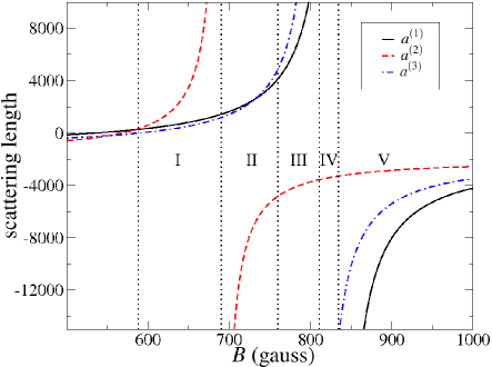
Figure 1: (color online) All possible s-wave scattering lengths are shown for the lowest 3 Zeeman states of Li⁶ from Ref. bartenstein2005pdl . Each marked region gives a different set of length scale discrepancies. Here $a^{\left(k\right)}$ is the scattering length between two atoms in states $\left|i\right\rangle$ and $\left|j\right\rangle$ with $k$ as the component not involved in the interaction.

Region
I	$r_{0}\ll a^{\left(3\right)}\lesssim a^{\left(1\right)}\ll a^{\left(2\right)}$	$a^{\left(1\right)},a^{\left(2\right)},a^{\left(3\right)}>0$
II	$r_{0}\ll a^{\left(3\right)}\sim a^{\left(1\right)}\ll\left|a^{\left(2\right)}\right|$	$a^{\left(2\right)}<0;a^{\left(1\right)},a^{\left(3\right)}>0$
III	$r_{0}\ll\left|a^{\left(2\right)}\right|\ll a^{\left(1\right)},a^{\left(3\right)}$	$a^{\left(2\right)}<0;a^{\left(1\right)},a^{\left(3\right)}>0$
IV	$r_{0}\ll\left|a^{\left(2\right)}\right|\ll\left|a^{\left(1\right)}\right|,a^{\left(3\right)}$	$a^{\left(2\right)},a^{\left(1\right)}<0;a^{\left(3\right)}>0$
V	$r_{0}\ll\left|a^{\left(2\right)}\right|\ll\left|a^{\left(1\right)}\right|\ll\left|a^{\left(3\right)}\right|$	$a^{\left(1\right)},a^{\left(2\right)},a^{\left(3\right)}<0$

Table 2: The possible tunable interaction regimes near the resonances of ⁶Li are given.

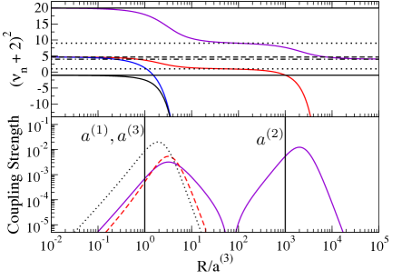
Figure 2: (color online) (a) For an example system having $a^{(1)}=a^{(3)}$ and $a^{(2)}=1000a^{(1)}$, the first four hyperangular eigenvalues are shown as functions of the hyperradius. The solid black horizontal lines show the expected behavior for 3 identical resonantly interacting bosons. The dashed line gives the behavior of two identical fermions interacting resonantly with a third distinguishable particle. Dotted lines give the expected universal behavior for a single resonant scattering length. Finally, the dot-dashed line is the lowest expected free space eigenvalue for three distinguishable free particles.(b)The coupling strengths between the third and fourth (purple solid curve), the first and fourth (red dashed curve), and the first and third (black dotted curve) adiabatic potentials are shown as a function of $R$.

Figure 2(a) shows an example of the lowest four hyperangular eigenvalues $\left(\nu+2\right)^{2}$ obtained from solving Eq. (40) for $a^{\left(1\right)}=a^{\left(3\right)}$ and $a^{\left(2\right)}=1000a^{\left(1\right)}$. This is provided as an example that is qualitatively similar to the behavior of the system in region I. When the hyperradius is in a region where all other length scales are much different, the hyperangular eigenvalue $\left(\nu+2\right)^{2}$ becomes constant, or, in the case of 2-body bound states, becomes proportional to $R^{2}$. This behavior can be interpreted as giving a universal set of potential curves from Eq. (31). For example in region I where $r_{0}\ll a^{\left(3\right)}\lesssim a^{\left(1\right)}\ll a^{\left(2\right)}$ there are three hyperradial regions: $r_{0}\ll R\ll a^{\left(3\right)}\lesssim a^{\left(1\right)}\ll a^{\left(2\right)}$; $r_{0}\ll a^{\left(3\right)}\lesssim a^{\left(1\right)}\ll R\ll a^{\left(2\right)}$; and $r_{0}\ll a^{\left(3\right)}\lesssim a^{\left(1\right)}\ll a^{\left(2\right)}\ll R$. In each region the hyperangular eigenvalues take on the universal value that is expected for resonant interactions efimov1973 ; nielsen2001tbp ; dincao2005sls .

Figure 3 schematically shows the behavior of the first few hyperradial effective potentials from Eq. (31). The grey areas are the regions where potentials are transitioning from one universal behavior to the next. The zero-range pseudo-potential cannot describe the short range details of the interaction, meaning that the potentials found here are only valid for $R\gg r_{0}$ where $r_{0}$ is a short range parameter shown schematically as the labeled blue region of Fig. 3.

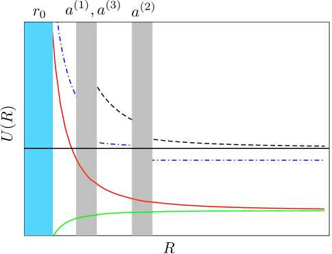
Figure 3: (color online) A schematic picture of the first four hyperradial potentials in region I is shown. The grey areas, labeled by the appropriate scattering lengths, indicate regions where the potentials are changing from one universal behavior to another. The blue region, labeled by $r_{0}$, indicates the short range region where the zero-range pseudo-potential not longer can be applied.

Figure 2(b) shows the coupling strength, $P_{mn}^{2}/2\mu\left[u_{m}\left(R\right)-u_{n}\left(R\right)\right]$, between the different potentials. The places where this coupling peaks are the points where a transition between curves is the most probable. Figures 4(a-e) are examples of the hyperangular eigenvalues found in each region. The magnetic field at which each set of eigenvalues are found is shown as dotted lines in Fig. 4(f) from left to right for Fig. 4(a-e) respectively. In each figure the hyperangular eigenvalue can be seen flattening out to a universal constant in each region of length scale discrepancy. As the magnetic field is scanned through each resonance, one two-body bound state becomes a virtual state. This behavior can be seen in the hyperangular eigenvalues that diverge toward $-\infty$. As each resonance is crossed, one of the hyperangular eigenvalue curves goes from diverging to $-\infty$ to converging to $\left(\nu+2\right)^{2}\rightarrow 4$.

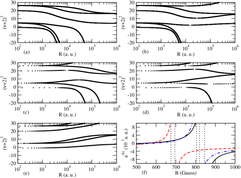
Figure 4: (color online) (a)-(e) Examples of the hyperangular eigenvalues from each region of magnetic field are shown as a function of the hyperradius in atomic units. (f) The three s-wave scattering lengths are shown as a reference plotted versus the magnetic field strength. The vertical dotted lines, from right to left, show the magnetic fields at which the hyperangular eigenvalues in (a)-(e) were found, $B=675,695,805,820$ and $845$ gauss respectively.

As a final examination of this system, we extract the scaling of the low energy three body recombination rate, i.e. the rate at which three particles collide and form a dimer and a free particle. The lowest 3-body curve, the lowest potential that goes to the three-free-particle threshold, is the potential that dominates this process. Contributions from higher hyperradial potentials will be suppressed due to larger tunneling barriers. One limitation of the zero-range pseudo-potential is that it only admits at most one dimer of each type. The process of three-body recombination releases the binding energy of the dimer state as kinetic energy between the dimer and remaining particle. For the purposes of this study we will concentrate on the three-body recombination processes that result in trap loss processes, where the energy released in the recombination can be assumed sufficient to eject the remaining fragments from a trap.

The event rate coefficient for $N$ initially unbound particles with total orbital angular momentum $L$ to make a transition from a hyperspherical potential curve with hyperangular eigenvalue $\lambda$ to a lower lying final state is given by mehta2009gtd ; esry1999rta

$$K_{N}=\dfrac{\hbar k}{\mu}N_{S}\left(\dfrac{2\pi}{k}\right)^{d-1}\dfrac{\Gamma\left(\dfrac{d}{2}\right)}{2\pi^{d/2}}\sum_{i,f}\left(2L+1\right)\left|T_{fi}\right|^{2},$$ (52)

where $d$ is the total dimension of the system (in the case of three-body recombination $d=6$), $T_{fi}\equiv S_{fi}-\delta_{fi}$ is the transition matrix element between an initial three-body entrance channel $i$ and a final exit channel $f$, and $k=\sqrt{2\mu E}/\hbar$ is the wave number of the asymptotic hyperradial wavefunction. The sum in this equation runs over all the initial, asymptotic channels with total angular momentum $L$ that contribute to the scattering process. In Eq. (52), $N_{S}$ is the number of permutational symmetries in the system. For three distinguishable particles $N_{S}=1$, but it can be different, for instance for $N$ identical bosons, $N_{S}=N!$.

In the low energy regime, only the lowest $L=0$ initial three-body channel will contribute, while higher channels will be suppressed. The sum over final $T$ matrix elements can be approximated using the Wentzel–Kramers–Brillouin (WKB) phase in the entrance channel mehta2009gtd ; dincao2005sls :

$$\sum_{f}\left|T_{fi}\right|^{2}\approx\dfrac{e^{-2\gamma}}{2}\dfrac{\sinh 2\eta}{\cos^{2}\phi+\sinh^{2}\eta},$$ (53)

where $\eta$ is an imaginary phase which parameterizes the losses from the incoming channel. In Eq. (53) $\gamma$ is the total WKB tunneling integral between the outer classical turning point and the hyperradial position at which the transition to the outgoing state occurs, i.e.

$$\gamma=\operatorname{Re}\left[\int_{R_{0}}^{R_{T}}\sqrt{\dfrac{2\mu}{\hbar^{2}}\left[U\left(R\right)-E\right]+\dfrac{1}{4R^{2}}}\;dR\right],$$ (54)

where $E$ is the initial three body energy, $R_{T}$ is the outer classical turning point and $R_{0}$ is the position at which the coupling between the incoming and outgoing channels peaks. In Eq. (53) $\phi$ is the WKB phase acumulated in any inner attractive well:

$$\phi=\operatorname{Im}\left[\int_{R_{0}}^{R_{T}}\sqrt{\dfrac{2\mu}{\hbar^{2}}\left[U\left(R\right)-E\right]+\dfrac{1}{4R^{2}}}\;dR\right].$$ (55)

The extra repulsive $1/4R^{2}$ term in Eqs. (54) and (55) is due to the Langer correction langer1937cfa . The total $T$-matrix element will depend on the detailed nature of the real short range interactions and the behavior of the outgoing channels, but the scaling behavior with the scattering lengths will be determined by Eq. (53). In each region of magnetic field, there are different length scale discrepancies and different numbers of bound states. As a result, we will examine each region separately.

IV.0.1 Region I $(a^{\left(1\right)}\sim a^{\left(3\right)}\ll a^{\left(2\right)})$

Figure 4(a) shows the behavior of the first few hyperangular eigenvalues in region I. The first three eigenvalues correspond to dimer states, while the fourth corresponds to the lowest three-body potential and is the entrance channel that will control three-body recombination. The lower two dimer states are relatively deeply bound with binding energies, $\hbar^{2}/ma^{2}$, on the order of $10^{-12}$ Hartree. This is comparable to the trap depth energy of a normal magneto-optical trap for experiments with ⁶Li ottenstein2008cst ; huckans2009tbr , meaning that recombination into these dimer channels typically releases enough energy to eject the remaining dimer-atom system from the trap.

In the limit where $R\gg a^{\left(3\right)}$, the three atoms are far enough apart to be in the non-interacting regime. This means that the hyperangular eigenfunction limits to the lowest allowed three-body hyperspherical harmonic with its corresponding eigenvalue, $\left(\nu+2\right)^{2}\rightarrow 4.$ In this limit the hyperradial potential becomes

$$U\left(R\gg a^{\left(3\right)}\right)=\dfrac{\hbar^{2}}{2\mu}\dfrac{4-1/4}{R^{2}}.$$ (56)

For very low energy scattering, the classical turning point in Eq. (53), is approximately

$$R_{T}=\dfrac{1}{2k}.$$ (57)

In fact, this will be the turning point for all of the three-body recombination processes discussed in this section.

It is possible for recombination to occur directly between the lowest three-body curve and the deep dimer channels, but this direct process is strongly suppressed due to the large tunneling barrier in the three-body potential at small $R$. The favored path is through a transition to the weakly bound dimer channel, shown schematically in Fig. 5.

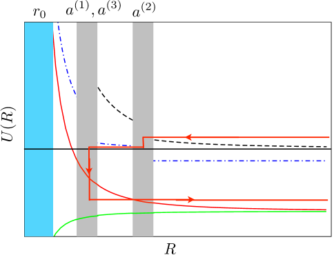
Figure 5: (Color online) A schematic of the path for three-body recombination in region I is shown. Transition regions are labeled by the appropriate length scale, and the short-range non-universal region is labeled by $r_{0}$.

The coupling between the lowest three-body channel and the weakly bound dimer channel peaks at approximately $R\sim a^{\left(2\right)}$, while the coupling peak between the weakly bound dimer channel and the remaining two dimer channels occurs at approximately $R\sim a^{\left(3\right)}$ $\sim a^{\left(1\right)}$. In the regime where $a^{\left(1\right)}\sim a^{\left(3\right)}\ll R\ll a^{\left(2\right)}$ the three particles are so far apart that they cannot see the smaller scattering lengths $a^{\left(1\right)}$ and $a^{\left(3\right)}$, but the third scattering length is so large compared to the hyperradius that it might as well be infinite. This leads to a universal potential whose hyperangular eigenvalue can be found by solving Eq. (40) with $a^{\left(1\right)}=a^{\left(3\right)}=0$ and $a^{\left(2\right)}\rightarrow\infty$, i.e

$$U\left(R\right) =\dfrac{\hbar^{2}}{2\mu}\dfrac{p_{1}^{2}-1/4}{R^{2}},$$ (58)

$$p_{1} =\left(\nu+2\right)=1.$$

This intermediate universal behavior can clearly be seen in Fig. (2a).

The behavior of each channel can be approximated by the universal behavior of the hyperradial potential in each region. Under this assumption, using Eq. (53), the tunneling probability is given by

$$e^{-2\gamma} \propto\exp\left[-2\int_{a^{\left(3\right)}}^{a^{\left(2\right)}}dR\sqrt{\dfrac{p_{1}^{2}}{R^{2}}-\frac{2\mu}{\hbar^{2}}E}\right.$$ (59)

$$-\left.2\int_{a^{\left(2\right)}}^{R_{T}}dR\sqrt{\dfrac{4}{R^{2}}-\frac{2\mu}{\hbar^{2}}E}\right].$$

If the scattering energy is very small, $E\ll\hbar^{2}/m\left[a^{\left(2\right)}\right]^{2}$, then the energy dependence in these integrands becomes negligible leaving,

$$e^{-2\gamma}\propto k^{4}\left(a^{\left(2\right)}a^{\left(3\right)}\right)^{2}.$$ (60)

Inserting this in for the $T$-matrix element in Eq. (52) gives the scaling behavior of the recombination rate with the scattering lengths dincao2005sls :

$$K_{3}\propto\left(a^{\left(2\right)}a^{\left(3\right)}\right)^{2}.$$ (61)

It was assumed here the final transition occurs at $R\sim a^{\left(3\right)}$ leading to the scaling behavior with $a^{\left(3\right)}$, but the transition could just as easily have occurred at $R\sim a^{\left(1\right)}$. $a^{\left(1\right)}$ and $a^{\left(3\right)}$ are approximately equal here, and which one dominates the transition depends on the short range behavior of the real two-body interaction. To extract the scaling behavior with respect to $a^{\left(1\right)}$, one can simply replace $a^{\left(3\right)}$ with $a^{\left(1\right)}$ in Eq. (61) as long as $a^{\left(1\right)}$ and $a^{\left(3\right)}$ are approximately equal.

IV.0.2 Region II $(a^{\left(1\right)}\sim a^{\left(3\right)}\ll\left|a^{\left(2\right)}\right|)$

The recombination in region II is simpler than in region I as there is no weakly bound intermediate state. Again, we assume that the trap loss recombination is dominated by transitions to the two remaining dimer states seen in Fig. 4(b). The lowest three-body potential has coupling to these channels that peaks at $R\sim a^{\left(1\right)}$ and $R\sim a^{\left(3\right)}$. For $R\gg\left|a^{\left(2\right)}\right|$ the hyperangular eigenvalue takes on the non-interacting value $\left(\nu+2\right)\rightarrow 2$. For $a^{\left(1\right)},a^{\left(3\right)}\ll R\ll\left|a^{\left(2\right)}\right|$ the universal hyperangular eigenvalue $\left(\nu+2\right)=p_{1}=1$ is seen again nielsen2001tbp ; dincao2005sls ; Braaten2006physrep . Ignoring the transitional region between these two regimes the transition probability is given by

$$e^{-2\gamma}\propto\exp\left[-2\left(\int_{a^{\left(3\right)}}^{\left|a^{\left(2\right)}\right|}dR\sqrt{\dfrac{p_{1}^{2}}{R^{2}}}+\int_{\left|a^{\left(2\right)}\right|}^{R_{T}}dR\sqrt{\dfrac{4}{R^{2}}}\right)\right].$$ (62)

Inserting this into Eq. (52) gives a recombination rate that has the same scaling behavior as in region I dincao2005sls :

$$K_{3}\propto\left(a^{\left(2\right)}a^{\left(3\right)}\right)^{2}.$$ (63)

Again it is assumed that the final transition occurs at $R\sim a^{\left(3\right)}$, but it could occur at $a^{\left(1\right)}$ as well. As in Region I, the scaling behavior with respect to $a^{\left(1\right)}$ can be found by simply replacing $a^{\left(3\right)}$ with $a^{\left(1\right)}$ in Eq. (61) as long as $a^{\left(1\right)}$ and $a^{\left(3\right)}$ are close.

IV.0.3 Region III $(\left|a^{\left(2\right)}\right|\ll a^{\left(1\right)}\sim a^{\left(3\right)})$ and Region IV $(\left|a^{\left(2\right)}\right|\ll\left|a^{\left(1\right)}\right|\sim a^{\left(3\right)})$

In Region III, none of the dimers predicted by the zero-range model have enough binding energy to cause trap loss. While recombination can occur into these channels, we will focus on the process of recombination to deeply bound states here. In reality, the deep interaction potential between two Li atom in different spin states admits many deeply bound dimer states, and a true hyperspherical description of the system would have channels going to each possible dimer-atom threshold. The energy released in recombining into these deep states is enough to kick the atoms out of any normal trap. Because the deeply bound states are of the size of the range of the interaction, coupling to the deeply bound hyperradial channels will peak at small hyperradius, $R\sim r_{0}$, and the rate can be found by studying the tunneling probability of reaching these states.

As with the recombination process in Region I, the most favorable pathway involves multiple steps. Starting from the lowest three-body channel, a transition is made to either the first or second weakly bound dimer channel. Because $a^{\left(1\right)}$ and $a^{\left(3\right)}$ are similar in magnitude, the coupling to these channels peaks in the same region. If the transition is made to the highest dimer channel, then another transition is made directly to the second.

This pathway is shown schematically in Fig. 6.

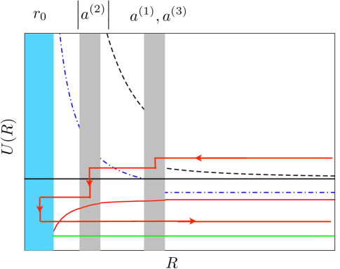
Figure 6: (color online) A schematic of the potentials and the path for three-body recombination in region III is shown. Again the labeled grey regions indicate a transition from one universal potential behavior to another. The green line represents the hyperradial potential for a deeply bound dimer state. The blue area labeled by $r_{0}$ is the short range region not described by zero-range interactions.

An interesting thing occurs in the lowest weakly bound potential when $\left|a^{\left(2\right)}\right|\ll R\ll a^{\left(1\right)}\sim a^{\left(3\right)}$: the universal potential becomes attractive. This region of attractive potential gives rise to a number of phenomena. For instance, in the limit $a^{\left(1\right)},a^{\left(3\right)}\rightarrow\infty$, the universal attractive potential supports an infinite number of geometrically spaced three-body bound states, giving rise to the Efimov effect. In the process of three-body recombination to deeply-bound dimer states, though, there is no tunnelling suppression in this channel, and the hyperradial wavefunction merely accumulates phase in this region. As a result the WKB tunnelling probability is controlled by the transition at $R\sim a^{\left(1\right)},a^{\left(3\right)}$:

$$e^{-2\gamma}\propto\exp\left[-2\int_{a^{\left(1\right)}}^{R_{T}}dR\sqrt{\dfrac{4}{R^{2}}}\right].$$ (64)

Inserting this into Eq. (52) gives the scaling of three-body recombination to deep dimer states as

$$K_{3}\propto\left[a^{\left(1\right)}\right]^{4}.$$ (65)

Again, it is assumed here that $a^{\left(1\right)}$ and $a^{\left(3\right)}$ are similar in magnitude. If this is not the case, for instance if $a^{\left(1\right)}\gg a^{\left(3\right)}$, then a scaling behavior similar to that of Eq. (61) is recovered:

$$K_{3}\propto\left[a^{\left(1\right)}a^{\left(3\right)}\right]^{2}.$$ (66)

In Region IV there is only a single weekly bound dimer state available, and trap loss will occur through recombination to deeply bound dimers. The path here is similar to that of Region III, where a transition happens from the lowest three-body channel to the weakly bound dimer channel. From there the hyperradial wavefunction can go to the small $R$ region without further suppression. This process then yields the same three-body recombination scaling behavior as Eq. (65) when $a^{\left(1\right)}\sim\left|a^{\left(3\right)}\right|$. When $a^{\left(3\right)}\gg\left|a^{\left(1\right)}\right|,$ the scaling predicted by Eq. (66) is recovered.

IV.0.4 Region V $(\left|a^{\left(2\right)}\right|\ll\left|a^{\left(3\right)}\right|\ll\left|a^{\left(1\right)}\right|)$

In this regime the recombination process is entirely controlled by the lowest three-body channel, shown schematically in Fig. 7.

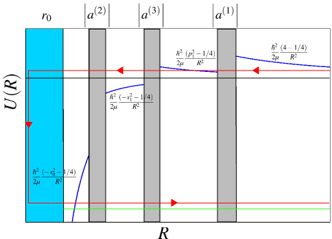
Figure 7: (Color online) A schematic of the lowest hyperradial potential is shown with the path for three-body recombination to deeply bound states. The green line represents the hyperradial potential for a deeply bound dimer state. Labeled grey areas indicate transition regions from one universal behavior to another, and the blue region indicates the short range regime.

The hyperradial potential has three universal regimes. The first, when $r_{0}\ll R\ll\left|a^{\left(2\right)}\right|\ll\left|a^{\left(3\right)}\right|\ll\left|a^{\left(1\right)}\right|$, is identical to that of three strongly interacting bosons. The hyperangular eigenvalue, $\left(\nu+2\right)^{2}$, is the first solution to Eq. (45) in the limit where $R/a\rightarrow 0$, yielding the hyperradial potential,

$$U\left(R\right) =\dfrac{\hbar^{2}}{2\mu}\dfrac{-\left(s_{0}\right)^{2}-1/4}{R^{2}},$$ (67)

$$s_{0} =1.0062.$$

In the next regime, when $r_{0}\ll\left|a^{\left(2\right)}\right|\ll R\ll\left|a^{\left(3\right)}\right|\ll\left|a^{\left(1\right)}\right|$, the three particles are far enough apart so as not to see the smallest scattering length. As a result the hyperangular eigenvalue is governed by Eq. (40) with the BBX symmetry of Table 1 imposed:

$$U\left(R\right) =\dfrac{\hbar^{2}}{2\mu}\dfrac{-\left(s_{1}\right)^{2}-1/4}{R^{2}},$$ (68)

$$s_{1} =0.4137.$$

In the regime where $r_{0}\ll\left|a^{\left(2\right)}\right|\ll\left|a^{\left(3\right)}\right|\ll R\ll\left|a^{\left(1\right)}\right|$, there is only one scattering length that is seen by the system, and the universal potential becomes that of Eq. (58). In the final regime, where the hyperradius is much larger than all of the scattering lengths, the potential goes to the non-interacting behavior of a hyperspherical harmonic.

The transition to a deeply bound dimer state occurs at $R\sim r_{0}$ following the path shown in Fig. 7. To get to this region, the wavefunction must first tunnel through a barrier, leading to suppression of the recombination rate. Once through the barrier, the wavefunction accumulates phase in the attractive potential regime. If enough phase can be accumulated in this regime, then a three-body bound state (a so called Efimov state) can be present leading to a resonance in the recombination rate. The final recombination rate for this process is esry1999rta ; nielsen2001tbp ; dincao2005sls ; braaten2004edr

$$K_{3}\propto A\dfrac{\sinh 2\eta}{\cos^{2}\left(\phi_{WKB}\right)+\sinh^{2}\eta},$$ (69)

where $\eta$ is controlled by the short range properties of the system, $\phi_{WKB}$ is the WKB phase accumulated in the attractive regime from $r_{0}$ to $\left|a^{\left(3\right)}\right|$, and $A$ is proportional to the tunneling suppression through the barrier:

$$A \propto\left[a^{\left(3\right)}a^{\left(1\right)}\right]^{2},$$ (70)

$$\phi_{WKB} =s_{1}\ln\left(\dfrac{a^{\left(3\right)}}{a^{\left(2\right)}}\right)+s_{0}\ln\left(\dfrac{\left|a^{\left(2\right)}\right|}{r_{0}}\right).$$ (71)

Figure 8 (a) show the log of the three-body recombination rate in arbitrary units as a function of the magnetic field with $\eta=0.001$. The short range length scale here is chosen to be approximately the van der Waals length of ⁶Li, $r_{0}=r_{d}\approx 30$ atomic units. Figure 8 (b) shows the scattering lengths in the same region of magnetic fields for reference.

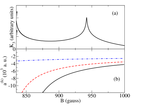
Figure 8: (color online) (a)The three-body recombination rate from Eq. (69) for ⁶Li is shown in arbitrary units as a function of magnetic field with $\eta=0.001$ and the short range length scale chosen to be approximately the van der Waals length, $r_{0}=r_{d}\approx 30$ a.u. The large y-axis tick marks indicate orders of maginitude. (b) The three scattering lengths $a^{\left(1\right)}$ (solid black curve), $a^{\left(2\right)}$ (dashed red curve) and $a^{\left(3\right)}$ (dot-dashed blue curve) are shown in atomic units as a function of magnetic field in Region V.

An Efimov resonance can clearly be seen at $B=942$ G when $\phi_{WKB}=3\pi/2$. This is in rough agreement with the predicted position of $B=1160$ G found in Ref. braaten2009three . The exact position of this resonance is somewhat sensitive to the short-range length scale $r_{0}$ which should be fit to experimental data. We have chosen $r_{0}$ as the Van der Waals length here for illustrative purposes. A WKB phase is $3\pi/2$ at the resonance indicates that this corresponds to the second Efimov state intersecting the continuum. The first Efimov state remains bound throughout this region. Because $a^{\left(1\right)}$ becomes resonantly large as  $B\rightarrow 834.15$ G, the $\left[a^{\left(3\right)}\right]^{2}$ scaling from Eq. (70) gives the large recombination rate seen in the lower field region of Fig. 8 (a).

With three overlapping resonances, ⁶Li provides a rich hunting ground for the study of three-body physics. Further, because it is a Fermionic atom, three-body interactions involving only two of the three lowest components are strongly suppressed meaning that the majority of the three-body physics is controlled by a system of three distinguishable particles. While only the processes of three-body recombination that lead to trap losses were studied in this section, there is still a rich and complex array of behaviors not discussed that can be described using the model presented here.

V Summary

In this work we have developed a new form for the hyperangular Green’s function in arbitrary dimensions. The derivation of the Green’s function is simple and follows easily from a standard Sturm-Liouville problem. By dividing a $d$ dimensional space into physically meaningful subspaces, this new Green’s function avoids the slow convergence often seen in spectral expansions form, while maintaining a physically intuitive set of hyperangular coordinates.

We have also used the hyperangular Green’s function to solve the three-body problem with zero-range s-wave interaction for arbitrary scattering lengths, particle masses and total angular momentum. With simple root finding, the adiabatic hyperangular channel functions and adiabatic potentials can be extracted. The resulting transcendental equation is in exact agreement with that derived using Fadeev like decompositions. To complete the problem, we have also derived, for the first time, general expressions for the non-adiabatic corrections to the potentials that are analytic up to root finding.

The results of the general three-body problem were then applied to the three lowest hyperfine components of ⁶Li near a set of overlapping resonances. By a simple WKB formalism, the scaling behavior of rate constant for trap loss three-body recombination events was extracted throughout the overlapping two-body resonances. Signatures of an Efimov style resonance are also predicted to appear at high field strengths. Throughout the resonances, all of the scattering lengths are very large compared to the length scale of the two-body interaction, indicating that the results presented here are universal. The simple and intuitive nature of the Lippmann-Schwinger equation in the three-body problem indicates that this Green’s function based method may be applicable in the context of the four-body problem, but this extension is the subject of ongoing inquiry.

Appendix A

In this appendix we sketch the derivation of the formulas for the non-adiabatic $\mathbf{P}$ and $\mathbf{Q}$ matrix elements given in Eqs.  (47) and (49). We begin by considering matrix elements dealing with the derivative of the Adiabatic Schrödinger equation:

$$\left\langle\Phi_{n}^{\prime}\left|\left(\Lambda^{2}-\varepsilon_{m}\right)\right|\Phi_{m}\right\rangle =0,$$ (72)

$$-\varepsilon_{n}^{\prime}\left\langle\Phi_{m}\left|\Phi_{n}\right.\right\rangle+\left\langle\Phi_{m}\left|\left(\Lambda^{2}-\varepsilon_{n}\right)\right|\Phi_{n}^{\prime}\right\rangle =0$$

where $\varepsilon_{n}=\nu_{n}\left(\nu_{n}+4\right)$ is the hyperangular eigenvalue of the $n$th adiabatic eigenfunction, and the prime indicates a hyperradial derivative has been taken. Taking the difference of these leads to an equation for the non-adiabatic coupling matrix element $P_{mn}$ for $m\neq n$:

$$\left\langle\Phi_{n}^{\prime}\left|\Lambda^{2}\right|\Phi_{m}\right\rangle-\left\langle\Phi_{m}\left|\Lambda^{2}\right|\Phi_{n}^{\prime}\right\rangle-\left(\varepsilon_{m}-\varepsilon_{n}\right)P_{mn}+\delta_{mn}\varepsilon_{n}^{\prime}=0.$$ (73)

The difference $\left\langle\Phi_{n}^{\prime}\left|\Lambda^{2}\right|\Phi_{m}\right\rangle-\left\langle\Phi_{m}\left|\Lambda^{2}\right|\Phi_{n}^{\prime}\right\rangle$ is given by the boundary conditions of the wave functions $\Phi_{m}$ and $\Phi_{n}$ at the coalescence points:

$$\left\langle\Phi_{n}^{\prime}\left|\Lambda^{2}\right|\Phi_{m}\right\rangle-\left\langle\Phi_{m}\left|\Lambda^{2}\right|\Phi_{n}^{\prime}\right\rangle =\sum_{k}\left[\dfrac{a^{\left(k\right)}}{d_{k}R}C_{m}\dfrac{\partial}{\partial R}C_{n}^{\left(k\right)}-C_{m}^{\left(k\right)}\dfrac{\partial}{\partial R}\left(\dfrac{a^{\left(k\right)}}{d_{k}R}C_{n}^{\left(k\right)}\right)\right]$$

$$=\sum_{k}C_{m}^{\left(k\right)}C_{n}^{\left(k\right)}\dfrac{a^{\left(k\right)}}{d_{k}R^{2}}.$$ (74)

Here the $LM$ subscript in the boundary values $C_{LM}^{\left(k\right)}$ have been suppressed. Inserting Eq. (74 into Eq. (73) yields Eq. (47),

$$P_{mn} =\dfrac{\sum_{k}C_{m}^{\left(k\right)}C_{n}^{\left(k\right)}\dfrac{a^{\left(k\right)}}{d_{k}R^{2}}}{\left(\varepsilon_{m}-\varepsilon_{n}\right)}\text{ for }n\neq m$$ (75)

$$-\varepsilon_{n}^{\prime} =\sum_{k}\left(C_{n}^{\left(k\right)}\right)^{2}\dfrac{a^{\left(k\right)}}{d_{k}R^{2}}.$$

A similar derivation provides the matrix elements $Q_{mn}$ given in Eq. (49).

References

(1)V. N. Efimov,
Sov. J. Nucl. Phys12, 589 (1971).
(2)V. N. Efimov,
Nucl. Phys. A210, 157 (1973).
(3)J. H. Macek,
Z. Phys. D3, 31 (1986).
(4)B. D. Esry, C. H. Greene, and J. P. Burke,
Phys. Rev. Lett.83, 1751 (1999).
(5)E. Nielsen and J. H. Macek,
Phys. Rev. Lett.83, 1566 (1999).
(6)E. Braaten and H. W. Hammer,
Phys. Rev. A70 (2004).
(7)T. Kraemer, M. Mark, P. Waldburger, J. G. Danzl, C. Chin, B. Engeser, A. D. Lange, K. Pilch, A. Jaakkola, H. Nägerl, and R. Grimm,
Nature440, 315 (2006).
(8)M. Zaccanti, B. Deissler, C. D’Errico, M. Fattori, M. Jona-Lasinio, S. Müller, G. Roati, M. Inguscio, and
G. Modugno,
Nature Phys.5, 586 (2009).
(9)T. B. Ottenstein, T. Lompe, M. Kohnen, A. N. Wenz, and
S. Jochim,
Phys. Rev. Lett.101, 203202 (2008).
(10)J. Huckans, J. Williams, E. Hazlett, R. Stites, and
K. O’Hara,
Phys. Rev. Lett.102, 165302 (2009).
(11)N. Gross, Z. Shotan, S. Kokkelmans, and L. Khaykovich,
Phys. Rev. Lett.103, 163202 (2009).
(12)S. E. Pollack, D. Dries, and R. G. Hulet,
Science326, 1683 (2009).
(13)J. von Stecher, J. P. D’Incao, and C. H. Greene,
Nature Physics5, 417 (2009).
(14)F. Ferlaino, S. Knoop, M. Berninger, W. Harm, J. P. D’Incao, H. C. Nägerl, and R. Grimm,
Phys. Rev. Lett.102, 140401 (2009).
(15)U. Fano,
Phys. Rev. A24, 2402 (1981).
(16)U. Fano,
Phys. Today29, 32 (1976).
(17)C. W. Clark and C. H. Greene,
Phys. Rev. A21, 1786 (1980).
(19)Y. Zhou, C. D. Lin, and J. Shertzer,
J. Phys. B26, 3937 (1993).
(20)C. D. Lin,
Phys. Rep.257, 1 (1995).
(21)V. Kokoouline and C. H. Greene,
Phys. Rev. A68, 012703 (2003).
(22)M. Fabre de la Ripelle,
Few-Body Systems14, 1 (1993).
(23)R. Szmytkowski,
J. Math. Phys.47, 063506 (2006).
(24)Y. F. Smirnov and K. V. Shitikova,
Sov. J. Part. Nucl.8, 44 (1977).
(25)J. Jackson,
Classical Electrodynamics Third Ed.,
John Wiley and Sons, New York, NY, 1999.
(26)M. Abramowitz and I. Stegun,
Handbook of Mathematical Functions, With Formulas, Graphs, and
Mathematical Tables,
Dover Publications, New York, NY, 1965.
(27)E. Nielsen, D. V. Fedorov, A. S. Jensen, and E. Garrido,
Phys. Rep.347, 373 (2001).
(28)J. P. D’Incao and B. D. Esry,
Phys. Rev. Lett.94, 213201 (2005).
(29)E. Braaten and H.-W. Hammer,
Phys. Rep.428, 259 (2006).
(30)M. Ross and G. Shaw,
Ann. Phys.13, 147 (1961).
(31)V. Efimov,
Physics Letters B33, 563 (1970).
(32)O. I. Kartavtsev and A. V. Malykh,
J. Phys. B40, 1429 (2007).
(33)E. Braaten, H. W. Hammer, D. Kang, and L. Platter,
Phys. Rev. Lett.103, 73202 (2009).
(34)P. Naidon and M. Ueda,
Phys. Rev. Lett.103, 73203 (2009).
(35)J. P. D’Incao and B. D. Esry,
Phys. Rev. Lett.103, 83202 (2009).
(36)S. T. Rittenhouse,
Phys. Rev. A81, 040701(R) (2010).
(37)M. Bartenstein, A. Altmeyer, S. Riedl, R. Geursen, S. Jochim, C. Chin, J. H. Denschlag, R. Grimm, A. Simoni, E. Tiesinga, et al.,
Phys. Rev. Lett.94, 103201 (2005).
(38)N. P. Mehta, S. T. Rittenhouse, J. P. D’Incao, J. von
Stecher, and C. H. Greene,
Phys. Rev. Lett.103, 153201 (2009).
(39)R. Langer,
Phys. Rev.51, 669 (1937).