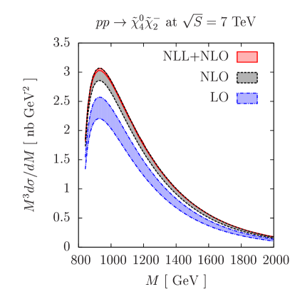
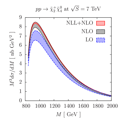
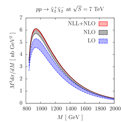
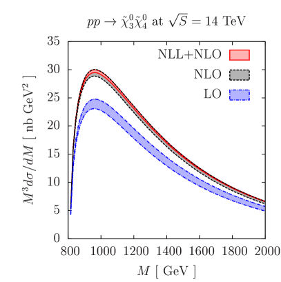
Threshold Resummation for Gaugino Pair Production at Hadron Colliders

Jonathan Debovea    Benjamin Fuksb    Michael Klasena klasen@lpsc.in2p3.fr a Laboratoire de Physique Subatomique et de Cosmologie, Université Joseph Fourier/CNRS-IN2P3/INPG, 53 Avenue des Martyrs, F-38026 Grenoble, France
b Institut Pluridisciplinaire Hubert Curien/Département Recherche Subatomique, Université de Strasbourg/CNRS-IN2P3, 23 Rue du Loess, F-67037 Strasbourg, France
Abstract

We present a complete analysis of threshold resummation effects on direct light and heavy gaugino pair production at the Tevatron and the LHC. Based on a new perturbative calculation at next-to-leading order of SUSY-QCD, which includes also squark mixing effects, we resum soft gluon radiation in the threshold region at leading and next-to-leading logarithmic accuracy, retaining at the same time the full SUSY-QCD corrections in the finite coefficient function. This allows us to correctly match the resummed to the perturbative cross section. Universal subleading logarithms are resummed in full matrix form. We find that threshold resummation slightly increases and considerably stabilizes the invariant mass spectra and total cross sections with respect to the next-to-leading order calculation. For future reference, we present total cross sections and their theoretical errors in tabular form for several commonly used SUSY benchmark points, gaugino pairs, and hadron collider energies.

pacs:
12.38.Cy,12.60.Jv,13.85.Qk,14.80.Ly
preprint: IPHC-PHENO-10-02preprint: LPSC 10-050

IPHC-PHENO-10-02
LPSC 10-050

I Introduction

The Minimal Supersymmetric Standard Model (MSSM) Nilles:1983ge continues to be one of the best-motivated and most intensely studied extensions of the Standard Model (SM) of particle physics. It introduces a symmetry between fermionic and bosonic degrees of freedom in nature and predicts one fermionic (bosonic) supersymmetric (SUSY) partner for each bosonic (fermionic) SM particle. Consequently, it allows to stabilize the gap between the electroweak and the Planck scale Witten:1981nf and to unify the three gauge couplings at energies of 𝒪(1016)𝒪superscript1016{\cal O}(10^{16}) GeV Dimopoulos:1981yj . It also contains a stable lightest supersymmetric particle (LSP), which interacts only weakly and represents therefore an excellent candidate for cold dark matter Ellis:1983ew . Spin partners of the SM particles have not yet been observed, and in order to remain a viable solution to the hierarchy problem, SUSY must be broken at low energy via soft terms in the Lagrangian. As a consequence, the SUSY particles must be massive in comparison to their SM counterparts, and the Tevatron and the LHC will perform a conclusive search covering a wide range of masses up to the TeV scale.

The production of SUSY particles at hadron colliders has been studied at leading order (LO) of perturbative QCD since the 1980s Barger:1983wc . More recently, previously neglected electroweak contributions Bozzi:2005sy , polarization effects Gehrmann:2004xu , and the violation of flavor Bozzi:2007me and CP𝐶𝑃CP symmetry Alan:2007rp have been considered at this order. Next-to-leading order (NLO) corrections have been computed within QCD since the late 1990s Beenakker:1996ch ; Beenakker:1999xh and recently also within the electroweak theory Hollik:2007wf . Resummation at the next-to-leading logarithmic (NLL) level has been achieved in the small transverse-momentum region for sleptons and gauginos Bozzi:2006fw , in the threshold region for sleptons, squarks and gluinos Bozzi:2007qr , and for sleptons and additional neutral gauge bosons also in both regions simultaneously Bozzi:2007tea .

As the fermionic partners of the electroweak gauge and Higgs bosons, the four neutralino (χ~i0(\tilde{\chi}^{0}_{i}, i=1,,4𝑖14i=1,\dots,4) and chargino (χ~i±(\tilde{\chi}^{\pm}_{i}, i=1,2𝑖12i=1,2) mass eigenstates are superpositions of the neutral and charged gaugino and higgsino interaction eigenstates. Their decays into leptons and missing transverse energy, carried away by the χ~10subscriptsuperscript~𝜒01\tilde{\chi}^{0}_{1} LSP, are easily identifiable at hadron colliders. The lighter mass eigenstates are accessible not only at the LHC with center-of-mass energies S𝑆\sqrt{S} of 7 to 14 TeV, but also at Run II of the Tevatron (S=1.96𝑆1.96\sqrt{S}=1.96 TeV), where the production of χ~1±χ~20subscriptsuperscript~𝜒plus-or-minus1subscriptsuperscript~𝜒02\tilde{\chi}^{\pm}_{1}\tilde{\chi}^{0}_{2} pairs decaying into trilepton final states is a gold-plated SUSY discovery channel Aaltonen:2008pv . For this particular channel, threshold resummation has been studied previously within the minimal supergravity (mSUGRA) model Li:2007ih . It was found that threshold resummation could increase the total cross section by up to 4.7% at the Tevatron relative to the NLO prediction, i.e. was significant even relatively far from the hadronic production threshold.

In this work, we extend and improve on these published results in several respects. First, we extend the original NLO calculation Beenakker:1999xh by also including squark mixing effects. Second, we include not only the QCD, but also the SUSY-QCD virtual loop contributions in the hard coefficient function of the resummed cross section, which therefore reproduces, when expanded, the correct NLO SUSY-QCD cross section in the threshold region. Third, we resum not only the diagonal, but the full matrix contributions coming from the anomalous dimension, thereby including all universal subleading terms and full singlet mixing. However, we refrain from resumming constant terms that are known to factorize and exponentiate in Drell-Yan like processes, but not in more complex processes like gaugino pair production with several interfering Born diagrams. For the Tevatron, we consider not only the production of χ~1±χ~20subscriptsuperscript~𝜒plus-or-minus1subscriptsuperscript~𝜒02\tilde{\chi}^{\pm}_{1}\tilde{\chi}^{0}_{2}, but also of χ~20χ~20subscriptsuperscript~𝜒02subscriptsuperscript~𝜒02\tilde{\chi}^{0}_{2}\tilde{\chi}^{0}_{2} and χ~1±χ~1±subscriptsuperscript~𝜒plus-or-minus1subscriptsuperscript~𝜒plus-or-minus1\tilde{\chi}^{\pm}_{1}\tilde{\chi}^{\pm}_{1} pairs. In particular the latter can have significantly larger cross sections than trilepton production due to the s𝑠s-channel exchange of massless photons. For the LHC, we concentrate on predictions for its initial center-of-mass energy of S=𝑆absent\sqrt{S}=7 TeV and include also the production of heavy gaugino (χ~2±subscriptsuperscript~𝜒plus-or-minus2\tilde{\chi}^{\pm}_{2}, χ~3,40subscriptsuperscript~𝜒034\tilde{\chi}^{0}_{3,4}) combinations, where threshold effects and direct gaugino pair production (as opposed to the production from squark and gluino cascade decays) will be more important. However, we will also show cross sections for S=𝑆absent\sqrt{S}=14 TeV for comparison.

The remainder of this paper is organized as follows: In Sec. II, we present briefly our LO and NLO SUSY-QCD calculations, focusing on squark mixing, the ultraviolet renormalization procedure and the dipole subtraction method employed for the cancellation of infrared divergences among virtual and real contributions. In Sec. III, we describe the threshold resummation formalism in Mellin space, starting from the refactorization of the perturbative cross section and the exponentiation of the eikonal function, giving then the explicit form of the resummed logarithms at NLL order, and finally describing various ways to improve on the original formalism. Sec. IV contains numerical results for various gaugino pair production cross sections at the Tevatron and at the LHC in both graphical and tabular form. It also includes a comprehensive analysis of theoretical errors coming from scale and parton density uncertainties. We summarize our results in Sec. V. Our conventions for the couplings of quarks and squarks to weak gauge bosons and gauginos are defined in the Appendix.

II Gaugino pair production at fixed order in perturbative QCD

At hadron colliders, two gauginos χ~i,jsubscript~𝜒𝑖𝑗\tilde{\chi}_{i,j} with masses mχ~i,jsubscript𝑚subscript~𝜒𝑖𝑗m_{\tilde{\chi}_{i,j}} and four-momenta p1,2subscript𝑝12p_{1,2} can be produced at LO of perturbation theory only through the annihilation of quarks q𝑞q and antiquarks q¯superscript¯𝑞\bar{q}^{\prime} with four-momenta pa,bsubscript𝑝𝑎𝑏p_{a,b},

q(pa)q¯(pb)𝑞subscript𝑝𝑎superscript¯𝑞subscript𝑝𝑏\displaystyle q(p_{a})\ \bar{q}^{\prime}(p_{b}) \displaystyle\to χ~i(p1)χ~j(p2),subscript~𝜒𝑖subscript𝑝1subscript~𝜒𝑗subscript𝑝2\displaystyle\tilde{\chi}_{i}(p_{1})\ \tilde{\chi}_{j}(p_{2}), (1)

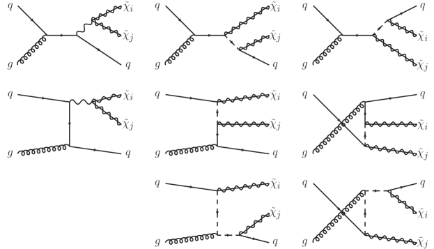
since gluons couple neither to electroweak gauge/Higgs bosons nor to their SUSY partners 111At the tree-level, we neglect s𝑠s-channel Higgs-boson exchanges, which may be produced by initial-state gluons through top-quark loops.. As shown in Fig. 1, the production can proceed either

Refer to caption
Figure 1: Tree-level Feynman diagrams for the production of gaugino pairs.

through the s𝑠s-channel exchange of a photon (γ𝛾\gamma), neutral (Z𝑍Z) or charged (W𝑊W) weak gauge boson, depending on the charge of the final state, or through the t𝑡t- and u𝑢u-channel exchange of a squark (q~~𝑞\tilde{q}), where the Mandelstam variables

s=(pa+pb)2𝑠superscriptsubscript𝑝𝑎subscript𝑝𝑏2\displaystyle s~{}=~{}(p_{a}+p_{b})^{2} , t=(pap1)2 , and u=(pap2)2𝑡superscriptsubscript𝑝𝑎subscript𝑝12 , and 𝑢superscriptsubscript𝑝𝑎subscript𝑝22\displaystyle t~{}=~{}(p_{a}-p_{1})^{2}\mbox{~{}~{},~{}and~{}~{}}u~{}=~{}(p_{a}-p_{2})^{2} (2)

and their mass-subtracted counterparts tχ~i,j=tmχ~i,j2subscript𝑡subscript~𝜒𝑖𝑗𝑡superscriptsubscript𝑚subscript~𝜒𝑖𝑗2t_{\tilde{\chi}_{i,j}}=t-m_{\tilde{\chi}_{i,j}}^{2} and uχ~i,j=umχ~i,j2subscript𝑢subscript~𝜒𝑖𝑗𝑢superscriptsubscript𝑚subscript~𝜒𝑖𝑗2u_{\tilde{\chi}_{i,j}}=u-m_{\tilde{\chi}_{i,j}}^{2} are defined in the usual way.

II.1 Leading order cross section

Table 1: s𝑠s-channel charges for gaugino pair production. The masses of the W𝑊W- and Z𝑍Z-bosons are mWsubscript𝑚𝑊m_{W} and mZsubscript𝑚𝑍m_{Z}.
QLsusuperscriptsubscript𝑄𝐿𝑠𝑢Q_{L}^{su} QLstsuperscriptsubscript𝑄𝐿𝑠𝑡Q_{L}^{st} QRsusuperscriptsubscript𝑄𝑅𝑠𝑢Q_{R}^{su} QRstsuperscriptsubscript𝑄𝑅𝑠𝑡Q_{R}^{st}
χ~i0χ~j0superscriptsubscript~𝜒𝑖0superscriptsubscript~𝜒𝑗0\tilde{\chi}_{i}^{0}\tilde{\chi}_{j}^{0} LqqZOij′′LsmZ2subscript𝐿𝑞superscript𝑞𝑍subscriptsuperscript𝑂′′𝐿𝑖𝑗𝑠subscriptsuperscript𝑚2𝑍\frac{L_{qq^{\prime}Z}O^{\prime\prime L}_{ij}}{s-m^{2}_{Z}} LqqZOij′′RsmZ2subscript𝐿𝑞superscript𝑞𝑍subscriptsuperscript𝑂′′𝑅𝑖𝑗𝑠subscriptsuperscript𝑚2𝑍\frac{L_{qq^{\prime}Z}O^{\prime\prime R}_{ij}}{s-m^{2}_{Z}} RqqZOij′′RsmZ2subscript𝑅𝑞superscript𝑞𝑍subscriptsuperscript𝑂′′𝑅𝑖𝑗𝑠subscriptsuperscript𝑚2𝑍\frac{R_{qq^{\prime}Z}O^{\prime\prime R}_{ij}}{s-m^{2}_{Z}} RqqZOij′′LsmZ2subscript𝑅𝑞superscript𝑞𝑍subscriptsuperscript𝑂′′𝐿𝑖𝑗𝑠subscriptsuperscript𝑚2𝑍\frac{R_{qq^{\prime}Z}O^{\prime\prime L}_{ij}}{s-m^{2}_{Z}}
χ~i+χ~j0superscriptsubscript~𝜒𝑖superscriptsubscript~𝜒𝑗0\tilde{\chi}_{i}^{+}\tilde{\chi}_{j}^{0} LqqWOjiLsmW2superscriptsubscript𝐿𝑞superscript𝑞𝑊subscriptsuperscript𝑂𝐿𝑗𝑖𝑠subscriptsuperscript𝑚2𝑊\frac{L_{qq^{\prime}W}^{\ast}O^{L\ast}_{ji}}{s-m^{2}_{W}} LqqWOjiRsmW2superscriptsubscript𝐿𝑞superscript𝑞𝑊subscriptsuperscript𝑂𝑅𝑗𝑖𝑠subscriptsuperscript𝑚2𝑊\frac{L_{qq^{\prime}W}^{\ast}O^{R\ast}_{ji}}{s-m^{2}_{W}} 0 0
χ~i+χ~jsuperscriptsubscript~𝜒𝑖superscriptsubscript~𝜒𝑗\tilde{\chi}_{i}^{+}\tilde{\chi}_{j}^{-} eqxWδqqδij4s+LqqZOijLsmZ2subscript𝑒𝑞subscript𝑥𝑊subscript𝛿𝑞superscript𝑞subscript𝛿𝑖𝑗4𝑠subscript𝐿𝑞superscript𝑞𝑍subscriptsuperscript𝑂𝐿𝑖𝑗𝑠subscriptsuperscript𝑚2𝑍-\frac{e_{q}x_{W}\delta_{qq^{\prime}}\delta_{ij}}{4s}+\frac{L_{qq^{\prime}Z}O^{\prime L}_{ij}}{s-m^{2}_{Z}}~{} eqxWδqqδij4s+LqqZOijRsmZ2subscript𝑒𝑞subscript𝑥𝑊subscript𝛿𝑞superscript𝑞subscript𝛿𝑖𝑗4𝑠subscript𝐿𝑞superscript𝑞𝑍subscriptsuperscript𝑂𝑅𝑖𝑗𝑠subscriptsuperscript𝑚2𝑍-\frac{e_{q}x_{W}\delta_{qq^{\prime}}\delta_{ij}}{4s}+\frac{L_{qq^{\prime}Z}O^{\prime R}_{ij}}{s-m^{2}_{Z}}~{} eqxWδqqδij4s+RqqZOijRsmZ2subscript𝑒𝑞subscript𝑥𝑊subscript𝛿𝑞superscript𝑞subscript𝛿𝑖𝑗4𝑠subscript𝑅𝑞superscript𝑞𝑍subscriptsuperscript𝑂𝑅𝑖𝑗𝑠subscriptsuperscript𝑚2𝑍-\frac{e_{q}x_{W}\delta_{qq^{\prime}}\delta_{ij}}{4s}+\frac{R_{qq^{\prime}Z}O^{\prime R}_{ij}}{s-m^{2}_{Z}}~{} eqxWδqqδij4s+RqqZOijLsmZ2subscript𝑒𝑞subscript𝑥𝑊subscript𝛿𝑞superscript𝑞subscript𝛿𝑖𝑗4𝑠subscript𝑅𝑞superscript𝑞𝑍subscriptsuperscript𝑂𝐿𝑖𝑗𝑠subscriptsuperscript𝑚2𝑍-\frac{e_{q}x_{W}\delta_{qq^{\prime}}\delta_{ij}}{4s}+\frac{R_{qq^{\prime}Z}O^{\prime L}_{ij}}{s-m^{2}_{Z}}

The LO differential cross section for given (anti-)quark helicities ha,bsubscript𝑎𝑏h_{a,b} can be expressed in the compact form

dσqq¯ha,hbdtdsuperscriptsubscript𝜎𝑞superscript¯𝑞subscript𝑎subscript𝑏d𝑡\displaystyle\frac{{\rm d}\sigma_{q\bar{q}^{\prime}}^{h_{a},h_{b}}}{{\rm d}t} =\displaystyle= 4πα2CA(1+δχiχj)xW2s2{(1ha)(1+hb)[|QLLu|2uχ~iuχ~j+|QLLt|2tχ~itχ~j+2Re[QLLuQLLt]mχ~imχ~js]\displaystyle\frac{4\pi\alpha^{2}}{C_{A}(1+\delta_{\chi_{i}\chi_{j}})x_{W}^{2}s^{2}}\Big{\{}(1-h_{a})(1+h_{b})\Big{[}\left|Q^{u}_{LL}\right|^{2}u_{\tilde{\chi}_{i}}u_{\tilde{\chi}_{j}}+\left|Q_{LL}^{t}\right|^{2}t_{\tilde{\chi}_{i}}t_{\tilde{\chi}_{j}}+2{\rm Re}[Q_{LL}^{u\ast}Q_{LL}^{t}]m_{\tilde{\chi}_{i}}m_{\tilde{\chi}_{j}}s\Big{]}
+(1+ha)(1hb)[|QRRu|2uχ~iuχ~j+|QRRt|2tχ~itχ~j+2Re[QRRuQRRt]mχ~imχ~js]1subscript𝑎1subscript𝑏delimited-[]superscriptsuperscriptsubscript𝑄𝑅𝑅𝑢2subscript𝑢subscript~𝜒𝑖subscript𝑢subscript~𝜒𝑗superscriptsuperscriptsubscript𝑄𝑅𝑅𝑡2subscript𝑡subscript~𝜒𝑖subscript𝑡subscript~𝜒𝑗2Redelimited-[]superscriptsubscript𝑄𝑅𝑅𝑢superscriptsubscript𝑄𝑅𝑅𝑡subscript𝑚subscript~𝜒𝑖subscript𝑚subscript~𝜒𝑗𝑠\displaystyle\hskip 85.35826pt+(1+h_{a})(1-h_{b})\Big{[}\left|Q_{RR}^{u}\right|^{2}u_{\tilde{\chi}_{i}}u_{\tilde{\chi}_{j}}+\left|Q_{RR}^{t}\right|^{2}t_{\tilde{\chi}_{i}}t_{\tilde{\chi}_{j}}+2{\rm Re}[Q_{RR}^{u\ast}Q_{RR}^{t}]m_{\tilde{\chi}_{i}}m_{\tilde{\chi}_{j}}s\Big{]}
+(1+ha)(1+hb)[|QRLu|2uχ~iuχ~j+|QRLt|2tχ~itχ~j2Re[QRLuQRLt](utmχ~i2mχ~j2)]1subscript𝑎1subscript𝑏delimited-[]superscriptsuperscriptsubscript𝑄𝑅𝐿𝑢2subscript𝑢subscript~𝜒𝑖subscript𝑢subscript~𝜒𝑗superscriptsuperscriptsubscript𝑄𝑅𝐿𝑡2subscript𝑡subscript~𝜒𝑖subscript𝑡subscript~𝜒𝑗2Redelimited-[]superscriptsubscript𝑄𝑅𝐿𝑢superscriptsubscript𝑄𝑅𝐿𝑡𝑢𝑡subscriptsuperscript𝑚2subscript~𝜒𝑖subscriptsuperscript𝑚2subscript~𝜒𝑗\displaystyle\hskip 85.35826pt+(1+h_{a})(1+h_{b})\Big{[}\left|Q_{RL}^{u}\right|^{2}u_{\tilde{\chi}_{i}}u_{\tilde{\chi}_{j}}+\left|Q_{RL}^{t}\right|^{2}t_{\tilde{\chi}_{i}}t_{\tilde{\chi}_{j}}-2{\rm Re}[Q_{RL}^{u\ast}Q_{RL}^{t}](ut-m^{2}_{\tilde{\chi}_{i}}m^{2}_{\tilde{\chi}_{j}})\Big{]}
+(1ha)(1hb)[|QLRu|2uχ~iuχ~j+|QLRt|2tχ~itχ~j2Re[QLRuQLRt](utmχ~i2mχ~j2)]}\displaystyle\hskip 85.35826pt+(1-h_{a})(1-h_{b})\Big{[}\left|Q_{LR}^{u}\right|^{2}u_{\tilde{\chi}_{i}}u_{\tilde{\chi}_{j}}+\left|Q_{LR}^{t}\right|^{2}t_{\tilde{\chi}_{i}}t_{\tilde{\chi}_{j}}-2{\rm Re}[Q_{LR}^{u\ast}Q_{LR}^{t}](ut-m^{2}_{\tilde{\chi}_{i}}m^{2}_{\tilde{\chi}_{j}})\Big{]}\Big{\}}

by employing the generalized charges

QXYt=2QXstδXYq~Xq~qχ~iYq~qχ~jtmq~2superscriptsubscript𝑄𝑋𝑌𝑡2superscriptsubscript𝑄𝑋𝑠𝑡subscript𝛿𝑋𝑌subscript~𝑞subscriptsuperscript𝑋~𝑞𝑞subscript~𝜒𝑖subscript𝑌~𝑞superscript𝑞subscript~𝜒𝑗𝑡subscriptsuperscript𝑚2~𝑞\displaystyle Q_{XY}^{t}~{}=~{}2Q_{X}^{st}\delta_{XY}-\sum_{\tilde{q}}\frac{X^{\ast}_{\tilde{q}q\tilde{\chi}_{i}}Y_{\tilde{q}q^{\prime}\tilde{\chi}_{j}}}{t-m^{2}_{\tilde{q}}} andand\displaystyle~{}~{}{\rm and}~{}~{} QXYu=2QXsuδXY+q~Xq~qχ~jYq~qχ~iumq~2,superscriptsubscript𝑄𝑋𝑌𝑢2superscriptsubscript𝑄𝑋𝑠𝑢subscript𝛿𝑋𝑌subscript~𝑞subscriptsuperscript𝑋~𝑞𝑞subscript~𝜒𝑗subscript𝑌~𝑞superscript𝑞subscript~𝜒𝑖𝑢subscriptsuperscript𝑚2~𝑞\displaystyle Q_{XY}^{u}~{}=~{}2Q_{X}^{su}\delta_{XY}+\sum_{\tilde{q}}\frac{X^{\ast}_{\tilde{q}q\tilde{\chi}_{j}}Y_{\tilde{q}q^{\prime}\tilde{\chi}_{i}}}{u-m^{2}_{\tilde{q}}}\ , (4)

where the s𝑠s-channel charges QXstsuperscriptsubscript𝑄𝑋𝑠𝑡Q_{X}^{st} and QXsusuperscriptsubscript𝑄𝑋𝑠𝑢Q_{X}^{su} are given in Tab. 1, mq~subscript𝑚~𝑞m_{\tilde{q}} is the mass of the squark exchanged in the t𝑡t- or u𝑢u-channel, X,Y{L,R}𝑋𝑌𝐿𝑅X,Y\in\{L,R\} relate to the left- and right-handed (s)quark couplings to weak gauge bosons and gauginos listed in App. A, and the couplings of the latter among each other depend on the neutral and charged gaugino-higgsino mixing matrices N𝑁N, U𝑈U and V𝑉V through the bilinear combinations Nilles:1983ge

OijL=122Ni4Vj212Ni2Vj1subscriptsuperscript𝑂𝐿𝑖𝑗122subscript𝑁𝑖4subscriptsuperscript𝑉𝑗212subscript𝑁𝑖2subscriptsuperscript𝑉𝑗1\displaystyle O^{L}_{ij}=\frac{1}{2\sqrt{2}}N_{i4}V^{\ast}_{j2}-\frac{1}{2}N_{i2}V^{\ast}_{j1} andand\displaystyle{\rm~{}~{}~{}~{}and~{}~{}~{}~{}} OijR=122Ni3Uj212Ni2Uj1,subscriptsuperscript𝑂𝑅𝑖𝑗122superscriptsubscript𝑁𝑖3subscript𝑈𝑗212superscriptsubscript𝑁𝑖2subscript𝑈𝑗1\displaystyle O^{R}_{ij}=-\frac{1}{2\sqrt{2}}N_{i3}^{\ast}U_{j2}-\frac{1}{2}N_{i2}^{\ast}U_{j1}\ ,~{} (5)
OijL=12cWVi1Vj1+14cWVi2Vj212cWδijxWsubscriptsuperscript𝑂𝐿𝑖𝑗12subscript𝑐𝑊subscript𝑉𝑖1superscriptsubscript𝑉𝑗114subscript𝑐𝑊subscript𝑉𝑖2superscriptsubscript𝑉𝑗212subscript𝑐𝑊subscript𝛿𝑖𝑗subscript𝑥𝑊\displaystyle O^{\prime L}_{ij}=\frac{1}{2c_{W}}V_{i1}V_{j1}^{\ast}+\frac{1}{4c_{W}}V_{i2}V_{j2}^{\ast}-\frac{1}{2c_{W}}\delta_{ij}x_{W} andand\displaystyle{\rm~{}~{}~{}~{}and~{}~{}~{}~{}} OijR=12cWUi1Uj1+14cWUi2Uj212cWδijxW,subscriptsuperscript𝑂𝑅𝑖𝑗12subscript𝑐𝑊superscriptsubscript𝑈𝑖1subscript𝑈𝑗114subscript𝑐𝑊superscriptsubscript𝑈𝑖2subscript𝑈𝑗212subscript𝑐𝑊subscript𝛿𝑖𝑗subscript𝑥𝑊\displaystyle O^{\prime R}_{ij}=\frac{1}{2c_{W}}U_{i1}^{\ast}U_{j1}+\frac{1}{4c_{W}}U_{i2}^{\ast}U_{j2}-\frac{1}{2c_{W}}\delta_{ij}x_{W}\ ,~{} (6)
Oij′′L=14cW[Ni3Nj3Ni4Nj4]subscriptsuperscript𝑂′′𝐿𝑖𝑗14subscript𝑐𝑊delimited-[]subscript𝑁𝑖3superscriptsubscript𝑁𝑗3subscript𝑁𝑖4superscriptsubscript𝑁𝑗4\displaystyle O^{\prime\prime L}_{ij}=\frac{1}{4c_{W}}\Big{[}N_{i3}N_{j3}^{\ast}-N_{i4}N_{j4}^{\ast}\Big{]} andand\displaystyle{\rm~{}~{}~{}~{}and~{}~{}~{}~{}} Oij′′R=14cW[Ni3Nj3+Ni4Nj4].subscriptsuperscript𝑂′′𝑅𝑖𝑗14subscript𝑐𝑊delimited-[]superscriptsubscript𝑁𝑖3subscript𝑁𝑗3superscriptsubscript𝑁𝑖4subscript𝑁𝑗4\displaystyle O^{\prime\prime R}_{ij}=\frac{1}{4c_{W}}\Big{[}-N_{i3}^{\ast}N_{j3}+N_{i4}^{\ast}N_{j4}\Big{]}\ .~{} (7)

α=e2/(4π)𝛼superscript𝑒24𝜋\alpha=e^{2}/(4\pi) is the electromagnetic fine structure constant, xW=1cW2=sW2=sin2θWsubscript𝑥𝑊1superscriptsubscript𝑐𝑊2superscriptsubscript𝑠𝑊2superscript2subscript𝜃𝑊x_{W}=1-c_{W}^{2}=s_{W}^{2}=\sin^{2}\theta_{W} is the squared sine of the electroweak mixing angle, and CA=3subscript𝐶𝐴3C_{A}=3, CF=4/3subscript𝐶𝐹43C_{F}=4/3 and αs=gs2/(4π)subscript𝛼𝑠superscriptsubscript𝑔𝑠24𝜋\alpha_{s}=g_{s}^{2}/(4\pi) are the QCD color factors and coupling constant. Unpolarized cross sections are obtained by averaging the polarized ones with

dσqq¯(0)dsuperscriptsubscript𝜎𝑞superscript¯𝑞0\displaystyle{\rm d}\sigma_{q\bar{q}^{\prime}}^{(0)} =\displaystyle= dσqq¯1,1+dσqq¯1,1+dσqq¯1,1+dσqq¯1,14.dsubscriptsuperscript𝜎11𝑞superscript¯𝑞dsubscriptsuperscript𝜎11𝑞superscript¯𝑞dsubscriptsuperscript𝜎11𝑞superscript¯𝑞dsubscriptsuperscript𝜎11𝑞superscript¯𝑞4\displaystyle\frac{{\rm d}\sigma^{1,1}_{q\bar{q}^{\prime}}+{\rm d}\sigma^{1,-1}_{q\bar{q}^{\prime}}+{\rm d}\sigma^{-1,1}_{q\bar{q}^{\prime}}+{\rm d}\sigma^{-1,-1}_{q\bar{q}^{\prime}}}{4}. (8)

II.2 Virtual corrections

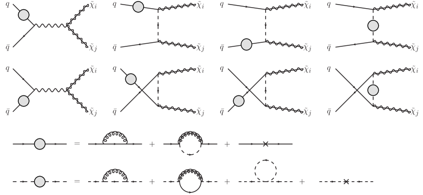
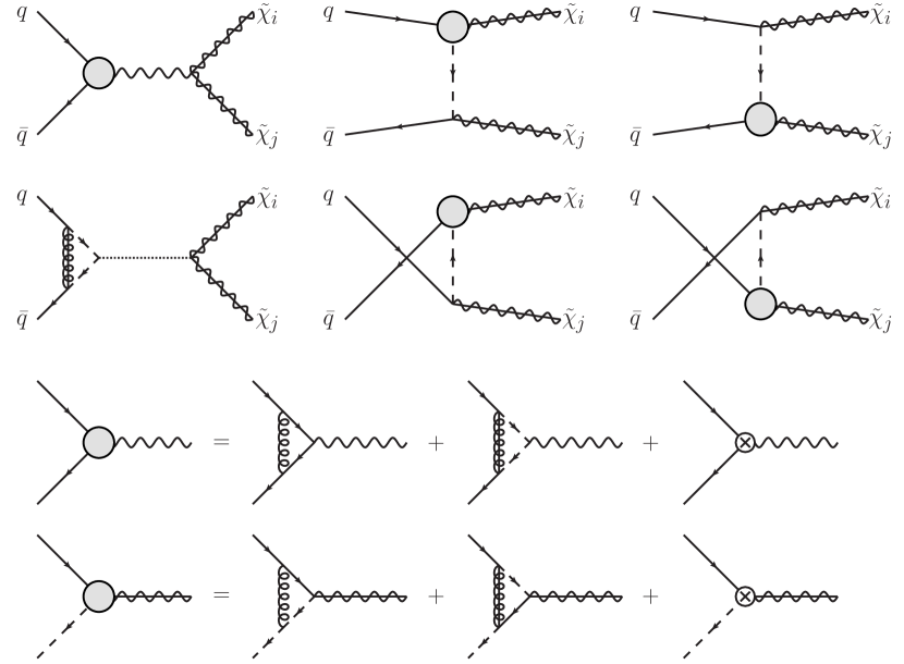
At NLO of SUSY-QCD, 𝒪(αs)𝒪subscript𝛼𝑠{\cal O}(\alpha_{s}), the cross section for gaugino pair production receives contributions from the interference of the virtual one-loop diagrams shown in Figs. 24 with the tree-level diagrams shown in Fig.
Refer to caption
Figure 2: Self-energy insertions (top) and contributions (bottom) to the production of gaugino pairs.

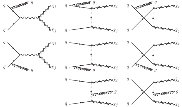
1 on the one hand and from real gluon (Fig. 5) and (anti-)quark emission diagrams on the other hand, where the latter are obtained by crossing the final-state gluon in Fig. 5 with the initial-state antiquark (Fig. 6) or quark (not shown). All diagrams have been evaluated analytically with self-written FORM programs and cross-checked independently with self-written MATHEMATICA programs.

The virtual self-energy diagrams for left- and right-handed quarks qL,R=PL,Rq=12(1γ5)qsubscript𝑞𝐿𝑅subscript𝑃𝐿𝑅𝑞12minus-or-plus1subscript𝛾5𝑞q_{L,R}=P_{L,R}\,q={1\over 2}(1\mp\gamma_{5})q (Fig. 2, third line),

ΣL,R(g)(p)subscriptsuperscriptΣ𝑔𝐿𝑅𝑝\displaystyle\Sigma^{(g)}_{L,R}(p) =\displaystyle= gs2CF16π2[(D2)B1(p,mq,0)+DmqB0(p,mq,0)]PL,R,superscriptsubscript𝑔𝑠2subscript𝐶𝐹16superscript𝜋2delimited-[]𝐷2italic-p̸subscript𝐵1𝑝subscript𝑚𝑞0𝐷subscript𝑚𝑞subscript𝐵0𝑝subscript𝑚𝑞0subscript𝑃𝐿𝑅\displaystyle-\frac{g_{s}^{2}C_{F}}{16\pi^{2}}\big{[}(D-2)\not{p}B_{1}(p,m_{q},0)+Dm_{q}B_{0}(p,m_{q},0)\big{]}P_{L,R}, (9)
ΣL(g~)(p)subscriptsuperscriptΣ~𝑔𝐿𝑝\displaystyle\Sigma^{(\tilde{g})}_{L~{}~{}\,}(p) =\displaystyle= gs2CF8π2i=12[B1(p,mg~,mq~i)Ri1q~Ri1q~+mg~B0(p,mg~,mq~i)Ri2q~Ri1q~]PL,andsuperscriptsubscript𝑔𝑠2subscript𝐶𝐹8superscript𝜋2superscriptsubscript𝑖12delimited-[]italic-p̸subscript𝐵1𝑝subscript𝑚~𝑔subscript𝑚subscript~𝑞𝑖superscriptsubscript𝑅𝑖1~𝑞superscriptsubscript𝑅𝑖1~𝑞subscript𝑚~𝑔subscript𝐵0𝑝subscript𝑚~𝑔subscript𝑚subscript~𝑞𝑖superscriptsubscript𝑅𝑖2~𝑞superscriptsubscript𝑅𝑖1~𝑞subscript𝑃𝐿and\displaystyle-\frac{g_{s}^{2}C_{F}}{8\pi^{2}}\sum_{i=1}^{2}\Big{[}\not{p}B_{1}(p,m_{\tilde{g}},m_{\tilde{q}_{i}})R_{i1}^{\tilde{q}\ast}R_{i1}^{\tilde{q}}+m_{\tilde{g}}B_{0}(p,m_{\tilde{g}},m_{\tilde{q}_{i}})R_{i2}^{\tilde{q}\ast}R_{i1}^{\tilde{q}}\Big{]}P_{L},~{}~{}{\rm and} (10)
ΣR(g~)(p)subscriptsuperscriptΣ~𝑔𝑅𝑝\displaystyle\Sigma^{(\tilde{g})}_{R~{}~{}\,}(p) =\displaystyle= gs2CF8π2i=12[B1(p,mg~,mq~i)Ri2q~Ri2q~+mg~B0(p,mg~,mq~i)Ri1q~Ri2q~]PR,superscriptsubscript𝑔𝑠2subscript𝐶𝐹8superscript𝜋2superscriptsubscript𝑖12delimited-[]italic-p̸subscript𝐵1𝑝subscript𝑚~𝑔subscript𝑚subscript~𝑞𝑖superscriptsubscript𝑅𝑖2~𝑞superscriptsubscript𝑅𝑖2~𝑞subscript𝑚~𝑔subscript𝐵0𝑝subscript𝑚~𝑔subscript𝑚subscript~𝑞𝑖superscriptsubscript𝑅𝑖1~𝑞superscriptsubscript𝑅𝑖2~𝑞subscript𝑃𝑅\displaystyle-\frac{g_{s}^{2}C_{F}}{8\pi^{2}}\sum_{i=1}^{2}\Big{[}\not{p}B_{1}(p,m_{\tilde{g}},m_{\tilde{q}_{i}})R_{i2}^{\tilde{q}\ast}R_{i2}^{\tilde{q}}+m_{\tilde{g}}B_{0}(p,m_{\tilde{g}},m_{\tilde{q}_{i}})R_{i1}^{\tilde{q}\ast}R_{i2}^{\tilde{q}}\Big{]}P_{R}, (11)

expanded as usual into vector (V) and scalar (S) parts Σ(p)=[ΣLV(p2)+ΣLS(p2)]PL+(LR)\Sigma(p)=[\Sigma^{V}_{L}(p^{2})\,\not{p}+\Sigma^{S}_{L}(p^{2})]P_{L}+(L\leftrightarrow R), as well as those for squarks (Fig. 2, fourth line),

Σij(g)(p2)subscriptsuperscriptΣ𝑔𝑖𝑗superscript𝑝2\displaystyle\Sigma^{(g)}_{ij}(p^{2}) =\displaystyle= gs2CF16π2[p2(B0(p,mq~i,0)2B1(p,mq~i,0)+B21(p,mq~i,0))+DB22(p,mq~i,0)]δij,superscriptsubscript𝑔𝑠2subscript𝐶𝐹16superscript𝜋2delimited-[]superscript𝑝2subscript𝐵0𝑝subscript𝑚subscript~𝑞𝑖02subscript𝐵1𝑝subscript𝑚subscript~𝑞𝑖0subscript𝐵21𝑝subscript𝑚subscript~𝑞𝑖0𝐷subscript𝐵22𝑝subscript𝑚subscript~𝑞𝑖0subscript𝛿𝑖𝑗\displaystyle-\frac{g_{s}^{2}C_{F}}{16\pi^{2}}\Big{[}p^{2}\big{(}B_{0}(p,m_{\tilde{q}_{i}},0)-2B_{1}(p,m_{\tilde{q}_{i}},0)+B_{21}(p,m_{\tilde{q}_{i}},0)\big{)}+DB_{22}(p,m_{\tilde{q}_{i}},0)\Big{]}\delta_{ij}, (12)
Σij(g~)(p2)subscriptsuperscriptΣ~𝑔𝑖𝑗superscript𝑝2\displaystyle\Sigma^{(\tilde{g})}_{ij}(p^{2}) =\displaystyle= gs2CF4π2{[p2(B1(p,mq,mg~)+B21(p,mq,mg~))+DB22(p,mq,mg~)]δij\displaystyle-\frac{g_{s}^{2}C_{F}}{4\pi^{2}}\Big{\{}\Big{[}p^{2}\big{(}B_{1}(p,m_{q},m_{\tilde{g}})+B_{21}(p,m_{q},m_{\tilde{g}})\big{)}+DB_{22}(p,m_{q},m_{\tilde{g}})\Big{]}\delta_{ij} (13)
mqmg~B0(p,mq,mg~)(Ri1q~Rj2q~+Ri2q~Rj1q~)},and\displaystyle\hskip 34.1433pt-~{}m_{q}m_{\tilde{g}}~{}B_{0}(p,m_{q},m_{\tilde{g}})\big{(}R_{i1}^{\tilde{q}}R_{j2}^{\tilde{q}\ast}+R_{i2}^{\tilde{q}}R_{j1}^{\tilde{q}\ast}\big{)}\Big{\}},~{}~{}{\rm and}
Σij(q~)(p2)subscriptsuperscriptΣ~𝑞𝑖𝑗superscript𝑝2\displaystyle\Sigma^{(\tilde{q})}_{ij}(p^{2}) =\displaystyle= gs2CF16π2k=12Skiq~Skjq~A0(mq~k)withSki=Rk1q~Ri1q~Rk2q~Ri2q~,superscriptsubscript𝑔𝑠2subscript𝐶𝐹16superscript𝜋2superscriptsubscript𝑘12superscriptsubscript𝑆𝑘𝑖~𝑞superscriptsubscript𝑆𝑘𝑗~𝑞subscript𝐴0subscript𝑚subscript~𝑞𝑘withsubscript𝑆𝑘𝑖subscriptsuperscript𝑅~𝑞𝑘1subscriptsuperscript𝑅~𝑞𝑖1subscriptsuperscript𝑅~𝑞𝑘2subscriptsuperscript𝑅~𝑞𝑖2\displaystyle\frac{g_{s}^{2}C_{F}}{16\pi^{2}}\sum_{k=1}^{2}S_{ki}^{\tilde{q}}S_{kj}^{\tilde{q}\ast}A_{0}(m_{\tilde{q}_{k}})~{}~{}~{}{\rm with}~{}~{}~{}S_{ki}=R^{\tilde{q}\ast}_{k1}R^{\tilde{q}}_{i1}-R^{\tilde{q}\ast}_{k2}R^{\tilde{q}}_{i2}, (14)

contain ultraviolet (UV) divergences in the scalar integrals B0,1,(p,m1,m2)subscript𝐵01𝑝subscript𝑚1subscript𝑚2B_{0,1,...}(p,m_{1},m_{2}) Passarino:1978jh , which exhibit themselves as 1/ϵ1italic-ϵ1/\epsilon poles in D=42ϵ𝐷42italic-ϵD=4-2\epsilon dimensions 222As it is customary, we absorb a factor of (2πμR)4Dsuperscript2𝜋subscript𝜇𝑅4𝐷(2\pi\mu_{R})^{4-D} in the definition of the scalar integrals, where μRsubscript𝜇𝑅\mu_{R} is the renormalization scale.. They must therefore be absorbed through a suitable
Refer to caption
Figure 3: Vertex correction insertions (top) and contributions (bottom) to the production of gaugino pairs.

renormalization procedure into the fundamental wave functions, mass parameters, and coupling constants of the SUSY-QCD Lagrangian

\displaystyle{\cal L} =\displaystyle= [q¯L0i∂̸qL0q¯R0mq0qL0+(LR)]+[i=12(μq~i0)(μq~i0)q~i0(mq~2)ii0q~i0]+.\displaystyle\Big{[}\bar{q}^{0}_{L}i\not{\partial}q^{0}_{L}-\bar{q}^{0}_{R}m^{0}_{q}q^{0}_{L}+(L\leftrightarrow R)\Big{]}+\Big{[}\sum_{i=1}^{2}(\partial_{\mu}\tilde{q}^{0}_{i})^{\dagger}(\partial^{\mu}\tilde{q}^{0}_{i})-\tilde{q}^{0\dagger}_{i}(m^{2}_{\tilde{q}})^{0}_{ii}\tilde{q}^{0}_{i}\Big{]}+\,...\,. (15)

The two components of the unrenormalized squark field q~0superscript~𝑞0\tilde{q}^{0} correspond originally to the left- and right-handed chiralities of the unrenormalized SM quark field q0superscript𝑞0q^{0}, but mix due to the fact that soft SUSY-breaking and Higgs terms render the 2×2222\times 2-dimensional mass matrix (mq~2)0superscriptsubscriptsuperscript𝑚2~𝑞0(m^{2}_{\tilde{q}})^{0} non-diagonal Nilles:1983ge . In Eq. (15) we have diagonalized this mass matrix with the squark rotation matrix Rq~ 0superscript𝑅~𝑞 0R^{\tilde{q}\,0}, so that the components i=1(2)𝑖12i=1\,(2) of the squark field correspond to the squark mass eigenvalues mq~i0superscriptsubscript𝑚subscript~𝑞𝑖0m_{\tilde{q}_{i}}^{0}. The squark self-energies in Eqs. (12)-(14) thus also carry indices i,j=1,2formulae-sequence𝑖𝑗12i,j=1,2 corresponding to the (outgoing and incoming) squark mass eigenstates. Multiplicative renormalization is achieved perturbatively by expanding the renormalization constants,

qL,R0=(1+12δZq)qL,Rsubscriptsuperscript𝑞0𝐿𝑅112𝛿subscript𝑍𝑞subscript𝑞𝐿𝑅\displaystyle q^{0}_{L,R}~{}=~{}\left(1~{}~{}+\frac{1}{2}\,\delta Z_{q}~{}~{}\right)q_{L,R}\, andand\displaystyle{\rm and} mq0=mq+δmq,\displaystyle~{}~{}m^{0}_{q}~{}~{}~{}\,=~{}~{}m_{q}~{}~{}~{}+~{}\delta m_{q}~{}~{}~{}\,, (16)
q~i0=(δij+12δZq~,ij)q~j\displaystyle\tilde{q}^{0}_{i}~{}~{}~{}\,=~{}\left(\delta_{ij}+\frac{1}{2}\,\delta Z_{\tilde{q},ij}\right)\tilde{q}_{j}~{}~{}~{} andand\displaystyle{\rm and} (mq~2)ij0=(mq~2)ij+(δmq~2)ij,subscriptsuperscriptsubscriptsuperscript𝑚2~𝑞0𝑖𝑗subscriptsubscriptsuperscript𝑚2~𝑞𝑖𝑗subscript𝛿subscriptsuperscript𝑚2~𝑞𝑖𝑗\displaystyle(m^{2}_{\tilde{q}})^{0}_{ij}~{}=~{}(m^{2}_{\tilde{q}})_{ij}+(\delta m^{2}_{\tilde{q}})_{ij}, (17)

with the usual factor of 1/2121/2 for the (s)quark wave functions. The renormalized self-energies are then

Σ^(p)^Σ𝑝\displaystyle\hat{\Sigma}(p) =\displaystyle= [ΣLV(p2)+12(δZq+δZq)]PL+[ΣLS(p2)12(mqδZq+δZqmq)δmq]PL+(LR)\displaystyle\Big{[}\Sigma^{V}_{L}(p^{2})+\frac{1}{2}(\delta Z_{q}+\delta Z_{q}^{\dagger})\Big{]}\not{p}P_{L}+\Big{[}\Sigma^{S}_{L}(p^{2})-\frac{1}{2}(m_{q}\delta Z_{q}+\delta Z_{q}^{\dagger}m_{q})-\delta m_{q}\Big{]}P_{L}+(L\leftrightarrow R) (18)

for quarks and

Σ^ij(p2)subscript^Σ𝑖𝑗superscript𝑝2\displaystyle\hat{\Sigma}_{ij}(p^{2}) =\displaystyle= Σij(p2)+12(δZq~,ij+δZq~,ji)p212k=12[(mq~2)ikδZq~,kj+δZq~,ki(mq~2)kj](δmq~2)ijsubscriptΣ𝑖𝑗superscript𝑝212𝛿subscript𝑍~𝑞𝑖𝑗𝛿subscriptsuperscript𝑍~𝑞𝑗𝑖superscript𝑝212superscriptsubscript𝑘12delimited-[]subscriptsuperscriptsubscript𝑚~𝑞2𝑖𝑘𝛿subscript𝑍~𝑞𝑘𝑗𝛿subscriptsuperscript𝑍~𝑞𝑘𝑖subscriptsuperscriptsubscript𝑚~𝑞2𝑘𝑗subscript𝛿superscriptsubscript𝑚~𝑞2𝑖𝑗\displaystyle\Sigma_{ij}(p^{2})+\frac{1}{2}(\delta Z_{\tilde{q},ij}+\delta Z^{\ast}_{\tilde{q},ji})\,p^{2}-\frac{1}{2}\sum_{k=1}^{2}\left[(m_{\tilde{q}}^{2})_{ik}\delta Z_{\tilde{q},kj}+\delta Z^{\ast}_{\tilde{q},ki}(m_{\tilde{q}}^{2})_{kj}\right]-(\delta m_{\tilde{q}}^{2})_{ij} (19)

for squarks.

We choose to renormalize the wave functions in the MS¯¯MS\overline{\rm MS}-scheme, so that the definition of the quark fields corresponds to the one employed in the parton densities in the external hadrons 333This is at variance with Ref. Li:2007ih , where the quark wave functions are renormalized on-shell, thereby absorbing finite SUSY contributions into the definition of the quark fields.. In this scheme, the quark wave function counterterm

δZq=δZq(g)+δZq(g~)𝛿subscript𝑍𝑞𝛿superscriptsubscript𝑍𝑞𝑔𝛿superscriptsubscript𝑍𝑞~𝑔\displaystyle\delta Z_{q}~{}=~{}\delta Z_{q}^{(g)}+\delta Z_{q}^{(\tilde{g})}~{} withwith\displaystyle{\rm with} δZq(g)=δZq(g~)=gs2CF16π2ΔandΔ=1ϵγE+ln4π,𝛿superscriptsubscript𝑍𝑞𝑔𝛿superscriptsubscript𝑍𝑞~𝑔superscriptsubscript𝑔𝑠2subscript𝐶𝐹16superscript𝜋2ΔandΔ1italic-ϵsubscript𝛾𝐸4𝜋\displaystyle~{}\delta Z_{q}^{(g)}~{}=~{}\delta Z_{q}^{(\tilde{g})}~{}=~{}-\frac{g_{s}^{2}C_{F}}{16\pi^{2}}\Delta~{}~{}{\rm and}~{}~{}\Delta~{}=~{}{1\over\epsilon}-\gamma_{E}+\ln 4\pi, (20)

defined as the UV-divergent plus universal finite parts of the on-shell counterterm ΣL,RV(mq2)mq2[ΣL,RV(mq2)+ΣR,LV(mq2)]mq[ΣL,RS(mq2)+ΣR,LS(mq2)]subscriptsuperscriptΣ𝑉𝐿𝑅superscriptsubscript𝑚𝑞2superscriptsubscript𝑚𝑞2delimited-[]subscriptsuperscriptΣ𝑉𝐿𝑅superscriptsubscript𝑚𝑞2subscriptsuperscriptΣ𝑉𝑅𝐿superscriptsubscript𝑚𝑞2subscript𝑚𝑞delimited-[]subscriptsuperscriptΣ𝑆𝐿𝑅superscriptsubscript𝑚𝑞2subscriptsuperscriptΣ𝑆𝑅𝐿superscriptsubscript𝑚𝑞2-\Sigma^{V}_{L,R}(m_{q}^{2})-m_{q}^{2}[\Sigma^{V\prime}_{L,R}(m_{q}^{2})+\Sigma^{V\prime}_{R,L}(m_{q}^{2})]-m_{q}[\Sigma^{S\prime}_{L,R}(m_{q}^{2})+\Sigma^{S\prime}_{R,L}(m_{q}^{2})] Bohm:2001yx , is hermitian (δZq=δZq𝛿subscript𝑍𝑞𝛿superscriptsubscript𝑍𝑞\delta Z_{q}=\delta Z_{q}^{\dagger}) and the same for left- and right-handed quarks. The superscripts g𝑔g and g~~𝑔\tilde{g} label the gluon and gluino exchange contributions, respectively, and γEsubscript𝛾𝐸\gamma_{E} is the Euler constant. The squark wave function counterterms

δZq~,ij𝛿subscript𝑍~𝑞𝑖𝑗\displaystyle\delta Z_{\tilde{q},ij} =\displaystyle= δZq~,ij(g)+δZq~,ij(g~)+δZq~,ij(q~),𝛿superscriptsubscript𝑍~𝑞𝑖𝑗𝑔𝛿superscriptsubscript𝑍~𝑞𝑖𝑗~𝑔𝛿superscriptsubscript𝑍~𝑞𝑖𝑗~𝑞\displaystyle\delta Z_{\tilde{q},ij}^{(g)}+\delta Z_{\tilde{q},ij}^{(\tilde{g})}+\delta Z_{\tilde{q},ij}^{(\tilde{q})}, (21)

with

δZq~,ii(g)=δZq~,ii(g~)=gs2CF8π2Δ𝛿superscriptsubscript𝑍~𝑞𝑖𝑖𝑔𝛿superscriptsubscript𝑍~𝑞𝑖𝑖~𝑔superscriptsubscript𝑔𝑠2subscript𝐶𝐹8superscript𝜋2Δ\displaystyle\delta Z_{\tilde{q},ii}^{(g)}~{}=~{}-\delta Z_{\tilde{q},ii}^{(\tilde{g})}~{}=~{}\frac{g_{s}^{2}C_{F}}{8\pi^{2}}\Delta~{} andand\displaystyle{\rm and} δZq~,ii(q~)=0𝛿superscriptsubscript𝑍~𝑞𝑖𝑖~𝑞0\displaystyle~{}\delta Z_{\tilde{q},ii}^{(\tilde{q})}~{}=~{}0 (22)

for i=j𝑖𝑗i=j and

δZq~,ij(g)𝛿subscriptsuperscript𝑍𝑔~𝑞𝑖𝑗\displaystyle\delta Z^{(g)}_{\tilde{q},ij} =\displaystyle= 0,0\displaystyle 0, (23)
δZq~,ij(g~)𝛿superscriptsubscript𝑍~𝑞𝑖𝑗~𝑔\displaystyle\delta Z_{\tilde{q},ij}^{(\tilde{g})} =\displaystyle= gs2CF4π22Δmq~i2mq~j2[mqmg~(Ri1q~Rj2q~+Ri2q~Rj1q~)],andsuperscriptsubscript𝑔𝑠2subscript𝐶𝐹4superscript𝜋22Δsuperscriptsubscript𝑚subscript~𝑞𝑖2superscriptsubscript𝑚subscript~𝑞𝑗2delimited-[]subscript𝑚𝑞subscript𝑚~𝑔subscriptsuperscript𝑅~𝑞𝑖1superscriptsubscript𝑅𝑗2~𝑞subscriptsuperscript𝑅~𝑞𝑖2superscriptsubscript𝑅𝑗1~𝑞and\displaystyle\frac{g_{s}^{2}C_{F}}{4\pi^{2}}\frac{2\Delta}{m_{\tilde{q}_{i}}^{2}-m_{\tilde{q}_{j}}^{2}}\Big{[}m_{q}m_{\tilde{g}}\big{(}R^{\tilde{q}}_{i1}R_{j2}^{\tilde{q}\ast}+R^{\tilde{q}}_{i2}R_{j1}^{\tilde{q}\ast}\big{)}\Big{]},~{}~{}{\rm and} (24)
δZq~,ij(q~)𝛿superscriptsubscript𝑍~𝑞𝑖𝑗~𝑞\displaystyle\delta Z_{\tilde{q},ij}^{(\tilde{q})} =\displaystyle= gs2CF16π22Δmq~i2mq~j2k=12mq~k2SkiSkjsuperscriptsubscript𝑔𝑠2subscript𝐶𝐹16superscript𝜋22Δsuperscriptsubscript𝑚subscript~𝑞𝑖2superscriptsubscript𝑚subscript~𝑞𝑗2superscriptsubscript𝑘12superscriptsubscript𝑚subscript~𝑞𝑘2subscript𝑆𝑘𝑖superscriptsubscript𝑆𝑘𝑗\displaystyle\frac{g_{s}^{2}C_{F}}{16\pi^{2}}\frac{2\Delta}{m_{\tilde{q}_{i}}^{2}-m_{\tilde{q}_{j}}^{2}}\sum_{k=1}^{2}m_{\tilde{q}_{k}}^{2}S_{ki}S_{kj}^{\ast} (25)

for ij𝑖𝑗i\neq j, defined similarly as the UV-divergent plus universal finite parts of the on-shell counterterms Re~Σii(mq~i2)~ResubscriptsuperscriptΣ𝑖𝑖superscriptsubscript𝑚subscript~𝑞𝑖2-\widetilde{\rm Re}\,\Sigma^{\prime}_{ii}(m_{\tilde{q}_{i}}^{2}) for i=j𝑖𝑗i=j and 2Re~Σij(mq~j2)/(mq~i2mq~j2)2~ResubscriptΣ𝑖𝑗superscriptsubscript𝑚subscript~𝑞𝑗2superscriptsubscript𝑚subscript~𝑞𝑖2superscriptsubscript𝑚subscript~𝑞𝑗22\,\widetilde{\rm Re}\,\Sigma_{ij}(m_{\tilde{q}_{j}}^{2})/(m_{\tilde{q}_{i}}^{2}-m_{\tilde{q}_{j}}^{2}) for ij𝑖𝑗i\neq j Bohm:2001yx , enter only through the renormalization of the squark mixing matrix,

Rq~ 0=Rq~+δRq~superscript𝑅~𝑞 0superscript𝑅~𝑞𝛿superscript𝑅~𝑞\displaystyle R^{\tilde{q}\,0}=R^{\tilde{q}}+\delta R^{\tilde{q}}~{} withwith\displaystyle{\rm with} δRijq~=14k=12(δZq~,ikδZq~,ki)Rkjq~=12k=12δZq~,ikRkjq~,𝛿superscriptsubscript𝑅𝑖𝑗~𝑞14superscriptsubscript𝑘12𝛿subscript𝑍~𝑞𝑖𝑘𝛿subscriptsuperscript𝑍~𝑞𝑘𝑖superscriptsubscript𝑅𝑘𝑗~𝑞12superscriptsubscript𝑘12𝛿subscript𝑍~𝑞𝑖𝑘superscriptsubscript𝑅𝑘𝑗~𝑞\displaystyle~{}\delta R_{ij}^{\tilde{q}}~{}=~{}\frac{1}{4}\sum_{k=1}^{2}(\delta Z_{\tilde{q},ik}-\delta Z^{\ast}_{\tilde{q},ki})R_{kj}^{\tilde{q}}~{}=~{}\frac{1}{2}\sum_{k=1}^{2}\delta Z_{\tilde{q},ik}R_{kj}^{\tilde{q}}, (26)

since in the MS¯¯MS\overline{\rm MS}-scheme the gluon and gluino contributions for i=j𝑖𝑗i=j in Eq. (22) cancel each other. In the last step of Eq. (26), we have made use of the fact that in the MS¯¯MS\overline{\rm MS}-scheme the squark wave-function renormalization constants are anti-hermitian matrices (δZq~,ij=δZq~,ji𝛿subscript𝑍~𝑞𝑖𝑗𝛿superscriptsubscript𝑍~𝑞𝑗𝑖\delta Z_{\tilde{q},ij}=-\delta Z_{\tilde{q},ji}^{\ast}).

Refer to caption
Figure 4: Box diagrams contributing to the production of gaugino pairs at NLO.

The (s)quark masses are renormalized in the on-shell scheme to make them correspond to the physical masses. The quark mass counterterm is then defined by mqΣV(mq2)+ΣS(mq2)subscript𝑚𝑞superscriptΣ𝑉superscriptsubscript𝑚𝑞2superscriptΣ𝑆superscriptsubscript𝑚𝑞2m_{q}\Sigma^{V}(m_{q}^{2})+\Sigma^{S}(m_{q}^{2}) Bohm:2001yx with the result

δmq𝛿subscript𝑚𝑞\displaystyle\delta m_{q} =\displaystyle= δmq(g)+δmq(g~)𝛿superscriptsubscript𝑚𝑞𝑔𝛿superscriptsubscript𝑚𝑞~𝑔\displaystyle\delta m_{q}^{(g)}+\delta m_{q}^{(\tilde{g})} (27)

and

δmq(g)𝛿superscriptsubscript𝑚𝑞𝑔\displaystyle\delta m_{q}^{(g)} =\displaystyle= gs2CF16π2mq[(D2)B1(mq,mq,0)+DB0(mq,mq,0)],superscriptsubscript𝑔𝑠2subscript𝐶𝐹16superscript𝜋2subscript𝑚𝑞delimited-[]𝐷2subscript𝐵1subscript𝑚𝑞subscript𝑚𝑞0𝐷subscript𝐵0subscript𝑚𝑞subscript𝑚𝑞0\displaystyle-\frac{g_{s}^{2}C_{F}}{16\pi^{2}}m_{q}\Big{[}(D-2)B_{1}(m_{q},m_{q},0)+DB_{0}(m_{q},m_{q},0)\Big{]}, (28)
δmq(g~)𝛿superscriptsubscript𝑚𝑞~𝑔\displaystyle\delta m_{q}^{(\tilde{g})} =\displaystyle= gs2CF16π2i=12[mqB1(mq,mg~,mq~i)+2mg~B0(mq,mg~,mq~i)Re(Ri2q~Ri1q~)].superscriptsubscript𝑔𝑠2subscript𝐶𝐹16superscript𝜋2superscriptsubscript𝑖12delimited-[]subscript𝑚𝑞subscript𝐵1subscript𝑚𝑞subscript𝑚~𝑔subscript𝑚subscript~𝑞𝑖2subscript𝑚~𝑔subscript𝐵0subscript𝑚𝑞subscript𝑚~𝑔subscript𝑚subscript~𝑞𝑖Resubscriptsuperscript𝑅~𝑞𝑖2subscriptsuperscript𝑅~𝑞𝑖1\displaystyle-\frac{g_{s}^{2}C_{F}}{16\pi^{2}}\sum_{i=1}^{2}\Big{[}m_{q}B_{1}(m_{q},m_{\tilde{g}},m_{\tilde{q}_{i}})+2m_{\tilde{g}}B_{0}(m_{q},m_{\tilde{g}},m_{\tilde{q}_{i}}){\rm Re}\big{(}R^{\tilde{q}\ast}_{i2}R^{\tilde{q}}_{i1}\big{)}\Big{]}. (29)

For our numerical results, we will set the masses of external quarks to zero in accordance with the collinear factorization of quarks in hadrons. The squark mass counterterm is defined by Re~[Σii(mq~i2)]~Redelimited-[]subscriptΣ𝑖𝑖superscriptsubscript𝑚subscript~𝑞𝑖2\widetilde{\rm Re}[\Sigma_{ii}(m_{\tilde{q}_{i}}^{2})]. The result is

δmq~i2𝛿superscriptsubscript𝑚subscript~𝑞𝑖2\displaystyle\delta m_{\tilde{q}_{i}}^{2} =\displaystyle= δmq~i2(g)+δmq~i2(g~)+δmq~i2(q~)𝛿superscriptsubscript𝑚subscript~𝑞𝑖2𝑔𝛿superscriptsubscript𝑚subscript~𝑞𝑖2~𝑔𝛿superscriptsubscript𝑚subscript~𝑞𝑖2~𝑞\displaystyle\delta m_{\tilde{q}_{i}}^{2(g)}+\delta m_{\tilde{q}_{i}}^{2(\tilde{g})}+\delta m_{\tilde{q}_{i}}^{2(\tilde{q})} (30)

with

δmq~i2(g)𝛿superscriptsubscript𝑚subscript~𝑞𝑖2𝑔\displaystyle\delta m_{\tilde{q}_{i}}^{2(g)} =\displaystyle= gs2CF8π2mq~i2[B1(mq~i,mq~i,0)B0(mq~i,mq~i,0)],superscriptsubscript𝑔𝑠2subscript𝐶𝐹8superscript𝜋2superscriptsubscript𝑚subscript~𝑞𝑖2delimited-[]subscript𝐵1subscript𝑚subscript~𝑞𝑖subscript𝑚subscript~𝑞𝑖0subscript𝐵0subscript𝑚subscript~𝑞𝑖subscript𝑚subscript~𝑞𝑖0\displaystyle\frac{g_{s}^{2}C_{F}}{8\pi^{2}}m_{\tilde{q}_{i}}^{2}\Big{[}B_{1}(m_{\tilde{q}_{i}},m_{\tilde{q}_{i}},0)-B_{0}(m_{\tilde{q}_{i}},m_{\tilde{q}_{i}},0)\Big{]}, (31)
δmq~i2(g~)𝛿superscriptsubscript𝑚subscript~𝑞𝑖2~𝑔\displaystyle\delta m_{\tilde{q}_{i}}^{2(\tilde{g})} =\displaystyle= gs2CF4π2[mq~i2B1(mq~i,mq,mg~)+mq2B0(mq~i,mq,mg~)+A0(mg~)\displaystyle-\frac{g_{s}^{2}C_{F}}{4\pi^{2}}\Big{[}m_{\tilde{q}_{i}}^{2}B_{1}(m_{\tilde{q}_{i}},m_{q},m_{\tilde{g}})+m_{q}^{2}B_{0}(m_{\tilde{q}_{i}},m_{q},m_{\tilde{g}})+A_{0}(m_{\tilde{g}}) (32)
 2mqmg~B0(mq~i,mq,mg~)Re(Ri1q~Ri2q~)],and\displaystyle\hskip 36.98857pt-\,2m_{q}m_{\tilde{g}}B_{0}(m_{\tilde{q}_{i}},m_{q},m_{\tilde{g}})\,{\rm Re}(R_{i1}^{\tilde{q}}R_{i2}^{\tilde{q}\ast})\Big{]},~{}~{}{\rm and}
δmq~i2(q~)𝛿superscriptsubscript𝑚subscript~𝑞𝑖2~𝑞\displaystyle\delta m_{\tilde{q}_{i}}^{2(\tilde{q})} =\displaystyle= gs2CF16π2j=12|Sji|2A0(mq~j).superscriptsubscript𝑔𝑠2subscript𝐶𝐹16superscript𝜋2superscriptsubscript𝑗12superscriptsubscript𝑆𝑗𝑖2subscript𝐴0subscript𝑚subscript~𝑞𝑗\displaystyle\frac{g_{s}^{2}C_{F}}{16\pi^{2}}\sum_{j=1}^{2}|S_{ji}|^{2}A_{0}(m_{\tilde{q}_{j}}). (33)

Supersymmetric Ward identities link the quark-quark-gauge boson and quark-squark-gaugino vertices to the weak gauge-boson and gaugino self-energies. As the latter do not receive strong corrections at NLO, the former require no further renormalization beyond the one for the (s)quark wave functions discussed above. However, the artificial breaking of supersymmetry by the mismatch of two gaugino and (D2)𝐷2(D-2) transverse vector degrees of freedom must be compensated by a finite counterterm g^=g[1αsCF/(8π)]^𝑔𝑔delimited-[]1subscript𝛼𝑠subscript𝐶𝐹8𝜋\hat{g}=g[1-\alpha_{s}C_{F}/(8\pi)], effectively shifting the quark-squark-gaugino scalar coupling constant g^^𝑔\hat{g} with respect to the weak gauge coupling constant g𝑔g Beenakker:1996ch ; AguilarSaavedra:2005pw .

II.3 Real corrections

Apart from the (now UV-finite) virtual corrections dσab(V)dsubscriptsuperscript𝜎𝑉𝑎𝑏{\rm d}\sigma^{(V)}_{ab} to the LO cross section dσab(0)dsubscriptsuperscript𝜎0𝑎𝑏{\rm d}\sigma^{(0)}_{ab} described above, the NLO cross section

dσab(1)(pa,pb)dsubscriptsuperscript𝜎1𝑎𝑏subscript𝑝𝑎subscript𝑝𝑏\displaystyle{\rm d}\sigma^{(1)}_{ab}(p_{a},p_{b}) =\displaystyle= 2+1[(dσab(R)(pa,pb))ϵ=0(dipolesdσab(0)(pa,pb)dVdipole)ϵ=0]subscript21delimited-[]subscriptdsubscriptsuperscript𝜎𝑅𝑎𝑏subscript𝑝𝑎subscript𝑝𝑏italic-ϵ0subscriptsubscriptdipolestensor-productdsubscriptsuperscript𝜎0𝑎𝑏subscript𝑝𝑎subscript𝑝𝑏dsubscript𝑉dipoleitalic-ϵ0\displaystyle\int_{2+1}\left[\left({\rm d}\sigma^{(R)}_{ab}(p_{a},p_{b})\right)_{\epsilon=0}-\left(\sum_{\mathrm{dipoles}}\;{\rm d}\sigma^{(0)}_{ab}(p_{a},p_{b})\otimes\;{\rm d}V_{\mathrm{dipole}}\right)_{\epsilon=0}\;\right] (34)
+\displaystyle+ 2[dσab(V)(pa,pb)+dσab(0)(pa,pb)𝑰]ϵ=0subscript2subscriptdelimited-[]dsubscriptsuperscript𝜎𝑉𝑎𝑏subscript𝑝𝑎subscript𝑝𝑏tensor-productdsubscriptsuperscript𝜎0𝑎𝑏subscript𝑝𝑎subscript𝑝𝑏𝑰italic-ϵ0\displaystyle\int_{2}\left[{\rm d}\sigma^{(V)}_{ab}(p_{a},p_{b})+{\rm d}\sigma^{(0)}_{ab}(p_{a},p_{b})\otimes{{\mbox{\boldmath$I$}}}\right]_{\epsilon=0}
+\displaystyle+ a01dx2[dσab(0)(xpa,pb)(𝑷+𝑲)a,a(x)+dσaa(0)(pa,xpb)(𝑷+𝑲)b,a(x)]ϵ=0subscriptsuperscript𝑎superscriptsubscript01differential-d𝑥subscript2subscriptdelimited-[]tensor-productdsubscriptsuperscript𝜎0superscript𝑎𝑏𝑥subscript𝑝𝑎subscript𝑝𝑏superscript𝑷𝑲𝑎superscript𝑎𝑥tensor-productdsubscriptsuperscript𝜎0𝑎superscript𝑎subscript𝑝𝑎𝑥subscript𝑝𝑏superscript𝑷𝑲𝑏superscript𝑎𝑥italic-ϵ0\displaystyle\sum_{a^{\prime}}\int_{0}^{1}{\rm d}x\;\int_{2}\left[{\rm d}\sigma^{(0)}_{a^{\prime}b}(xp_{a},p_{b})\otimes\left({{\mbox{\boldmath$P$}}}+{{\mbox{\boldmath$K$}}}\right)^{a,a^{\prime}}(x)+{\rm d}\sigma^{(0)}_{aa^{\prime}}(p_{a},xp_{b})\otimes\left({{\mbox{\boldmath$P$}}}+{{\mbox{\boldmath$K$}}}\right)^{b,a^{\prime}}(x)\right]_{\epsilon=0}

also receives contributions dσab(R)dsubscriptsuperscript𝜎𝑅𝑎𝑏{\rm d}\sigma^{(R)}_{ab} from real gluon (Fig. 5), quark (Fig. 6) and antiquark (not shown) emission
Refer to caption
Figure 5: Gluon emission diagrams contributing to the production of gaugino pairs at NLO.
Refer to caption
Figure 6: Quark emission diagrams contributing to the production of gaugino pairs at NLO.

diagrams, where the emitted parton carries four-momentum p3subscript𝑝3p_{3}. In the Catani-Seymour dipole formalism Catani:1996vz , the real contributions are rendered infrared (IR) finite by subtracting from them their soft and collinear limits (pa,bp30subscript𝑝𝑎𝑏subscript𝑝30p_{a,b}\cdot p_{3}\to 0)

dσab(0)(pa,pb)dVdipoletensor-productdsubscriptsuperscript𝜎0𝑎𝑏subscript𝑝𝑎subscript𝑝𝑏dsubscript𝑉dipole\displaystyle{\rm d}\sigma^{(0)}_{ab}(p_{a},p_{b})\otimes{\rm d}V_{\mathrm{dipole}} =\displaystyle= i[𝒟a3,b(p1,p2,p3;pa,pb)FJ(2)(p~1,p~2;p~a3,pb)+(ab)]\displaystyle\sum_{i}\left[{\cal D}^{a3,b}(p_{1},p_{2},p_{3};p_{a},p_{b})\;F_{J}^{(2)}({\widetilde{p}}_{1},{\widetilde{p}}_{2};{\widetilde{p}}_{a3},p_{b})+(a\leftrightarrow b)\right] (35)

before integration over the three-particle final-state phase space. They can then be evaluated in four dimensions (i.e. with ϵ=0italic-ϵ0\epsilon=0). In the case at hand of two initial-state partons and no colored final state particles at LO, the only dipole contribution comes from an initial state emitter and an initial state spectator, e.g.

𝒟a3,b(p1,p2,p3;pa,pb)superscript𝒟𝑎3𝑏subscript𝑝1subscript𝑝2subscript𝑝3subscript𝑝𝑎subscript𝑝𝑏\displaystyle{\cal D}^{a3,b}(p_{1},p_{2},p_{3};p_{a},p_{b}) =\displaystyle= 12pap31x3,ab1~,2~;a3~,b|𝑻b𝑻a3𝑻a32𝑽a3,b|1~,2~;a3~,b2,ab2,ab\displaystyle-\frac{1}{2p_{a}\cdot p_{3}}\;\frac{1}{x_{3,ab}}{}_{2,ab}\langle{{\widetilde{1}},{\widetilde{2}};{\widetilde{a3}},b}|\,\frac{{{\mbox{\boldmath$T$}}}_{b}\cdot{{\mbox{\boldmath$T$}}}_{a3}}{{{\mbox{\boldmath$T$}}}_{a3}^{2}}\;{{\mbox{\boldmath$V$}}}^{a3,b}\,|{{\widetilde{1}},{\widetilde{2}};{\widetilde{a3}},b}\rangle_{2,ab} (36)

(see Eq. (5.136) of Ref. Catani:1996vz ). The color charges 𝑻a3,bsubscript𝑻𝑎3𝑏{{\mbox{\boldmath$T$}}}_{a3,b} and splitting functions 𝑽a3,bsuperscript𝑽𝑎3𝑏{{\mbox{\boldmath$V$}}}^{a3,b} (Eqs. (5.145)-(5.148) of Ref. Catani:1996vz ) act on Born-like squared matrix elements, which are written here in terms of vectors |1~,2~;a3~,b2,absubscriptket~1~2~𝑎3𝑏2𝑎𝑏|{{\widetilde{1}},{\widetilde{2}};{\widetilde{a3}},b}\rangle_{2,ab} in color and helicity space. These matrix elements involve an initial-state parton a3~~𝑎3{\widetilde{a3}} with momentum parallel to pasubscript𝑝𝑎p_{a},

p~a3μ=x3,abpaμsuperscriptsubscript~𝑝𝑎3𝜇subscript𝑥3𝑎𝑏superscriptsubscript𝑝𝑎𝜇\displaystyle{\widetilde{p}}_{a3}^{\mu}~{}=~{}x_{3,ab}\,p_{a}^{\mu} ,where\displaystyle,~{}~{}{\rm where}~{}~{} x3,ab=papbp3pap3pbpapb,subscript𝑥3𝑎𝑏subscript𝑝𝑎subscript𝑝𝑏subscript𝑝3subscript𝑝𝑎subscript𝑝3subscript𝑝𝑏subscript𝑝𝑎subscript𝑝𝑏\displaystyle x_{3,ab}~{}=~{}\frac{p_{a}\cdot p_{b}-p_{3}\cdot p_{a}-p_{3}\cdot p_{b}}{p_{a}\cdot p_{b}}, (37)

and rescaled four-momenta of the final-state gauginos

p~1,2μ=p1,2μ2p1,2(K+K~)(K+K~)2(K+K~)μ+2p1,2KK2K~μ,superscriptsubscript~𝑝12𝜇superscriptsubscript𝑝12𝜇2subscript𝑝12𝐾~𝐾superscript𝐾~𝐾2superscript𝐾~𝐾𝜇2subscript𝑝12𝐾superscript𝐾2superscript~𝐾𝜇{\widetilde{p}_{1,2}}^{\mu}=p_{1,2}^{\mu}-\frac{2p_{1,2}\cdot(K+{\widetilde{K}})}{(K+{\widetilde{K}})^{2}}\;(K+{\widetilde{K}})^{\mu}+\frac{2p_{1,2}\cdot K}{K^{2}}\;{\widetilde{K}}^{\mu}, (38)

where Kμ=paμ+pbμp3μsuperscript𝐾𝜇superscriptsubscript𝑝𝑎𝜇superscriptsubscript𝑝𝑏𝜇superscriptsubscript𝑝3𝜇K^{\mu}=p_{a}^{\mu}+p_{b}^{\mu}-p_{3}^{\mu} and K~μ=p~a3μ+pbμsuperscript~𝐾𝜇superscriptsubscript~𝑝𝑎3𝜇superscriptsubscript𝑝𝑏𝜇{\widetilde{K}}^{\mu}={\widetilde{p}_{a3}}^{\mu}+p_{b}^{\mu}. The phase space function FJ(2)(p~1,p~2;p~a3,pb)superscriptsubscript𝐹𝐽2subscript~𝑝1subscript~𝑝2subscript~𝑝𝑎3subscript𝑝𝑏F_{J}^{(2)}({\widetilde{p}}_{1},{\widetilde{p}}_{2};{\widetilde{p}}_{a3},p_{b}) tends to zero with pap3subscript𝑝𝑎subscript𝑝3p_{a}\cdot p_{3} and ensures therefore that the LO cross section is IR-finite. To compensate for the subtracted auxiliary dipole term dσab(0)(pa,pb)dVdipoletensor-productdsubscriptsuperscript𝜎0𝑎𝑏subscript𝑝𝑎subscript𝑝𝑏dsubscript𝑉dipole{\rm d}\sigma^{(0)}_{ab}(p_{a},p_{b})\otimes{\rm d}V_{\mathrm{dipole}}, the latter must be integrated analytically over the full phase space of the emitted parton,

𝑰=dipoles1dVdipole,𝑰subscriptdipolessubscript1differential-dsubscript𝑉dipole{{\mbox{\boldmath$I$}}}=\sum_{\mathrm{dipoles}}\;\int_{1}\;{\rm d}V_{\mathrm{dipole}}\;\;, (39)

and added to the virtual cross section. The integrated dipole term is defined explicitly in Eq. (10.15) of Ref. Catani:1996vz ; it contains all the simple and double poles in ϵitalic-ϵ\epsilon necessary to cancel the IR singularities in dσab(V)dsubscriptsuperscript𝜎𝑉𝑎𝑏{\rm d}\sigma^{(V)}_{ab}. The insertion operators

𝑷a,a(p1,,pm,pb;xpa,x;μF2)superscript𝑷𝑎superscript𝑎subscript𝑝1subscript𝑝𝑚subscript𝑝𝑏𝑥subscript𝑝𝑎𝑥superscriptsubscript𝜇𝐹2\displaystyle{{\mbox{\boldmath$P$}}}^{a,a^{\prime}}(p_{1},...,p_{m},p_{b};xp_{a},x;\mu_{F}^{2}) =\displaystyle= αs2πPaa(x)1𝑻a2[i𝑻i𝑻alnμF22xpapi+𝑻b𝑻alnμF22xpapb]subscript𝛼𝑠2𝜋superscript𝑃𝑎superscript𝑎𝑥1superscriptsubscript𝑻superscript𝑎2delimited-[]subscript𝑖subscript𝑻𝑖subscript𝑻superscript𝑎superscriptsubscript𝜇𝐹22𝑥subscript𝑝𝑎subscript𝑝𝑖subscript𝑻𝑏subscript𝑻superscript𝑎superscriptsubscript𝜇𝐹22𝑥subscript𝑝𝑎subscript𝑝𝑏\displaystyle\frac{\alpha_{s}}{2\pi}\;P^{aa^{\prime}}(x)\;\frac{1}{{{\mbox{\boldmath$T$}}}_{a^{\prime}}^{2}}\left[\sum_{i}{{\mbox{\boldmath$T$}}}_{i}\cdot{{\mbox{\boldmath$T$}}}_{a^{\prime}}\;\ln\frac{\mu_{F}^{2}}{2xp_{a}\cdot p_{i}}+{{\mbox{\boldmath$T$}}}_{b}\cdot{{\mbox{\boldmath$T$}}}_{a^{\prime}}\;\ln\frac{\mu_{F}^{2}}{2xp_{a}\cdot p_{b}}\right] (40)

are directly related to the regularized Altarelli-Parisi splitting distributions at 𝒪(αs)𝒪subscript𝛼𝑠{\cal O}(\alpha_{s}),

Pqq(x)superscript𝑃𝑞𝑞𝑥\displaystyle P^{qq}(x) =\displaystyle= CF[1+x2(1x)++32δ(1x)],subscript𝐶𝐹delimited-[]1superscript𝑥2subscript1𝑥32𝛿1𝑥\displaystyle~{}C_{F}\left[\frac{1+x^{2}}{(1-x)_{+}}+{3\over 2}\delta(1-x)\right], (41)
Pqg(x)superscript𝑃𝑞𝑔𝑥\displaystyle P^{qg}(x) =\displaystyle= CF[1+(1x)2x],subscript𝐶𝐹delimited-[]1superscript1𝑥2𝑥\displaystyle~{}C_{F}\left[\frac{1+(1-x)^{2}}{x}\right], (42)
Pgq(x)superscript𝑃𝑔𝑞𝑥\displaystyle P^{gq}(x) =\displaystyle= TR[x2+(1x)2],andsubscript𝑇𝑅delimited-[]superscript𝑥2superscript1𝑥2and\displaystyle~{}T_{R}\;\left[x^{2}+(1-x)^{2}\right],~{}~{}{\rm and} (43)
Pgg(x)superscript𝑃𝑔𝑔𝑥\displaystyle P^{gg}(x) =\displaystyle= 2CA[(11x)++1xx1+x(1x)]+β0δ(1x),2subscript𝐶𝐴delimited-[]subscript11𝑥1𝑥𝑥1𝑥1𝑥subscript𝛽0𝛿1𝑥\displaystyle 2C_{A}\left[\left(\frac{1}{1-x}\right)_{+}+\frac{1-x}{x}-1+x(1-x)\right]+\beta_{0}\,\delta(1-x), (44)

where β0=11CA/62NfTR/3subscript𝛽011subscript𝐶𝐴62subscript𝑁𝑓subscript𝑇𝑅3\beta_{0}=11C_{A}/6-2N_{f}T_{R}/3 and β1=(17CA25CANf3CFNf)/6subscript𝛽117superscriptsubscript𝐶𝐴25subscript𝐶𝐴subscript𝑁𝑓3subscript𝐶𝐹subscript𝑁𝑓6\beta_{1}=(17C_{A}^{2}-5C_{A}N_{f}-3C_{F}N_{f})/6 are the one- and two-loop coefficients of the QCD beta-function, CF=4/3subscript𝐶𝐹43C_{F}=4/3, TR=1/2subscript𝑇𝑅12T_{R}=1/2, CA=3subscript𝐶𝐴3C_{A}=3, and Nfsubscript𝑁𝑓N_{f} is the number of quark flavors. They cancel the dependence of the hadronic cross section on the factorization scale μFsubscript𝜇𝐹\mu_{F} up to NLO accuracy. The insertion operators

𝑲a,a(x)=αs2π{K¯aa(x)KF.S.aa(x)+δaai𝑻i𝑻aγi(1)𝑻i2[(11x)++δ(1x)]}αs2π𝑻b𝑻a1𝑻a2K~aa(x)superscript𝑲𝑎superscript𝑎𝑥subscript𝛼𝑠2𝜋absentabsentsuperscript¯𝐾𝑎superscript𝑎𝑥subscriptsuperscript𝐾𝑎superscript𝑎formulae-sequenceFS𝑥superscript𝛿𝑎superscript𝑎subscript𝑖subscript𝑻𝑖subscript𝑻𝑎superscriptsubscript𝛾𝑖1superscriptsubscript𝑻𝑖2delimited-[]subscript11𝑥𝛿1𝑥subscript𝛼𝑠2𝜋subscript𝑻𝑏subscript𝑻superscript𝑎1superscriptsubscript𝑻superscript𝑎2superscript~𝐾𝑎superscript𝑎𝑥{{\mbox{\boldmath$K$}}}^{a,a^{\prime}}(x)=\frac{\alpha_{s}}{2\pi}\left\{\frac{}{}{\overline{K}}^{aa^{\prime}}(x)-K^{{aa^{\prime}}}_{\scriptscriptstyle\rm F\!.S\!.}(x)+\;\delta^{aa^{\prime}}\;\sum_{i}{{\mbox{\boldmath$T$}}}_{i}\cdot{{\mbox{\boldmath$T$}}}_{a}\;\frac{\gamma_{i}^{(1)}}{{{\mbox{\boldmath$T$}}}_{i}^{2}}\left[\left(\frac{1}{1-x}\right)_{+}+\delta(1-x)\right]\right\}-\frac{\alpha_{s}}{2\pi}{{\mbox{\boldmath$T$}}}_{b}\cdot{{\mbox{\boldmath$T$}}}_{a^{\prime}}\frac{1}{{{\mbox{\boldmath$T$}}}_{a^{\prime}}^{2}}{\widetilde{K}}^{aa^{\prime}}(x) (45)

with γq(1)=3CF/2superscriptsubscript𝛾𝑞13subscript𝐶𝐹2\gamma_{q}^{(1)}=3C_{F}/2 and γg(1)=β0superscriptsubscript𝛾𝑔1subscript𝛽0\gamma_{g}^{(1)}=\beta_{0},

K¯qq(x)=K¯q¯q¯(x)superscript¯𝐾𝑞𝑞𝑥superscript¯𝐾¯𝑞¯𝑞𝑥\displaystyle{\overline{K}}^{qq}(x)\;\,=\;\,{\overline{K}}^{{\bar{q}}{\bar{q}}}(x) =\displaystyle= CF[(21xln1xx)+(1+x)ln1xx+(1x)]δ(1x)(5π2)CF,subscript𝐶𝐹delimited-[]subscript21𝑥1𝑥𝑥1𝑥1𝑥𝑥1𝑥𝛿1𝑥5superscript𝜋2subscript𝐶𝐹\displaystyle C_{F}\left[\left(\frac{2}{1-x}\ln\frac{1-x}{x}\right)_{+}-(1+x)\ln\frac{1-x}{x}+(1-x)\right]-\delta(1-x)\left(5-\pi^{2}\right)C_{F}\;\;, (46)
K¯qg(x)=K¯q¯g(x)superscript¯𝐾𝑞𝑔𝑥superscript¯𝐾¯𝑞𝑔𝑥\displaystyle{\overline{K}}^{qg}(x)\;\,=\;\,{\overline{K}}^{{\bar{q}}g}(x) =\displaystyle= Pqg(x)ln1xx+CFx,superscript𝑃𝑞𝑔𝑥1𝑥𝑥subscript𝐶𝐹𝑥\displaystyle P^{qg}(x)\ln\frac{1-x}{x}+C_{F}\;x\;\;, (47)
K¯gq(x)=K¯gq¯(x)superscript¯𝐾𝑔𝑞𝑥superscript¯𝐾𝑔¯𝑞𝑥\displaystyle{\overline{K}}^{gq}(x)\;\,=\;\,{\overline{K}}^{g{\bar{q}}}(x) =\displaystyle= Pgq(x)ln1xx+TR 2x(1x),superscript𝑃𝑔𝑞𝑥1𝑥𝑥subscript𝑇𝑅2𝑥1𝑥\displaystyle P^{gq}(x)\ln\frac{1-x}{x}+T_{R}\;2x(1-x)\;\;, (48)
K¯gg(x)superscript¯𝐾𝑔𝑔𝑥\displaystyle{\overline{K}}^{gg}(x) =\displaystyle= 2CA[(11xln1xx)++(1xx1+x(1x))ln1xx]2subscript𝐶𝐴delimited-[]subscript11𝑥1𝑥𝑥1𝑥𝑥1𝑥1𝑥1𝑥𝑥\displaystyle 2C_{A}\left[\left(\frac{1}{1-x}\ln\frac{1-x}{x}\right)_{+}+\left(\frac{1-x}{x}-1+x(1-x)\right)\ln\frac{1-x}{x}\right] (49)
\displaystyle- δ(1x)[(509π2)CA169TRNf],𝛿1𝑥delimited-[]509superscript𝜋2subscript𝐶𝐴169subscript𝑇𝑅subscript𝑁𝑓\displaystyle\delta(1-x)\left[\left(\frac{50}{9}-\pi^{2}\right)C_{A}-\frac{16}{9}T_{R}N_{f}\right]\;\;,
K¯q¯q(x)=K¯qq¯(x)superscript¯𝐾¯𝑞𝑞𝑥superscript¯𝐾𝑞¯𝑞𝑥\displaystyle{\overline{K}}^{{\bar{q}}q}(x)\;\,=\;\,{\overline{K}}^{q{\bar{q}}}(x) =\displaystyle= 0,0\displaystyle 0, (50)

and

K~ab(x)superscript~𝐾𝑎𝑏𝑥\displaystyle{\widetilde{K}}^{ab}(x) =\displaystyle= Pregab(x)ln(1x)+δab𝑻a2[(21xln(1x))+π23δ(1x)]subscriptsuperscript𝑃𝑎𝑏reg𝑥1𝑥superscript𝛿𝑎𝑏superscriptsubscript𝑻𝑎2delimited-[]subscript21𝑥1𝑥superscript𝜋23𝛿1𝑥\displaystyle P^{ab}_{{\rm reg}}(x)\;\ln(1-x)+\;\delta^{ab}\,{{\mbox{\boldmath$T$}}}_{a}^{2}\left[\left(\frac{2}{1-x}\ln(1-x)\right)_{+}-\frac{\pi^{2}}{3}\delta(1-x)\right] (51)

depend on the factorization scheme through the term KF.S.aa(x)subscriptsuperscript𝐾𝑎superscript𝑎formulae-sequenceFS𝑥K^{{aa^{\prime}}}_{\scriptscriptstyle\rm F\!.S\!.}(x), which vanishes in the MS¯¯MS\overline{\rm MS}-scheme, and also on the regular parts of the Altarelli-Parisi splitting

Refer to caption
Figure 7: Associated production of a gaugino and a virtual squark, decaying subsequently into a gaugino and a quark.

distributions given by Pregab(x)=Pab(x)subscriptsuperscript𝑃𝑎𝑏reg𝑥superscript𝑃𝑎𝑏𝑥P^{ab}_{{\rm reg}}(x)=P^{ab}(x), if ab𝑎𝑏a\neq b, and otherwise by

Pregqq(x)=CF(1+x)subscriptsuperscript𝑃𝑞𝑞reg𝑥subscript𝐶𝐹1𝑥\displaystyle P^{qq}_{{\rm reg}}(x)~{}=~{}-C_{F}\,(1+x)~{}~{} andand\displaystyle{\rm and} Preggg(x)=2CA[1xx1+x(1x)].subscriptsuperscript𝑃𝑔𝑔reg𝑥2subscript𝐶𝐴delimited-[]1𝑥𝑥1𝑥1𝑥\displaystyle~{}~{}P^{gg}_{{\rm reg}}(x)~{}=~{}2\,C_{A}\left[\frac{1-x}{x}-1+x(1-x)\right]. (52)

The last line in Eq. (34) contains therefore the finite remainders that are left after the factorization of collinear initial-state singularities into the parton densities in the MS¯¯MS\overline{\rm MS}-scheme at the factorization scale μFsubscript𝜇𝐹\mu_{F}. As guaranteed by the Kinoshita-Lee-Nauenberg and factorization theorems, the total NLO cross section is then not only UV-, but also IR-finite.

Finally, one subtlety must still be addressed: in Fig. 6, the center and right diagrams of lines one and three proceed through a squark propagator, which can become on-shell if mq~mχ~subscript𝑚~𝑞subscript𝑚~𝜒m_{\tilde{q}}\geq m_{\tilde{\chi}} and s(mq~+mχ~)2𝑠superscriptsubscript𝑚~𝑞subscript𝑚~𝜒2s\geq(m_{\tilde{q}}+m_{\tilde{\chi}})^{2}. To avoid double counting, the resonance contribution

dσqg(q~)dsubscriptsuperscript𝜎~𝑞𝑞𝑔\displaystyle{\rm d}\sigma^{(\tilde{q})}_{qg} =\displaystyle= dσ(qgχ~q~)BR(q~χ~q)d𝜎𝑞𝑔~𝜒~𝑞BR~𝑞~𝜒𝑞\displaystyle{\rm d}\sigma(qg\to\tilde{\chi}\tilde{q})~{}{\rm BR}(\tilde{q}\to\tilde{\chi}q) (53)

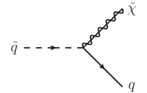
must be subtracted from the gaugino pair production process using the narrow-width approximation, as it is identified experimentally as the associated production of a gaugino and a squark (Fig. 7), followed by the decay of the squark into a gaugino and a quark (Fig. 8).

III Threshold Resummation at Next-to-Leading Logarithmic Accuracy

In the previous section, we have demonstrated that all soft and collinear (IR) singularities in the partonic NLO cross section dσab(1)dsubscriptsuperscript𝜎1𝑎𝑏{\rm d}\sigma^{(1)}_{ab} either cancel among virtual and real corrections or can be absorbed at the factorization scale μFsubscript𝜇𝐹\mu_{F} into parton density functions (PDFs) fa,b/A,B(xa,b,μF2)subscript𝑓𝑎𝑏𝐴𝐵subscript𝑥𝑎𝑏superscriptsubscript𝜇𝐹2f_{a,b/A,B}(x_{a,b},\mu_{F}^{2}), which represent probability distributions for initial partons a,b𝑎𝑏a,b with longitudinal momentum fraction xa,bsubscript𝑥𝑎𝑏x_{a,b} in the external hadrons A,B𝐴𝐵A,B (e.g. protons or anti-protons). The QCD factorization theorem guarantees that the observable hadronic cross section

M2dσABdM2(τ)superscript𝑀2dsubscript𝜎𝐴𝐵dsuperscript𝑀2𝜏\displaystyle M^{2}\frac{{\rm d}\sigma_{AB}}{{\rm d}M^{2}}(\tau) =\displaystyle= ab01dxadxbdz[xafa/A(xa,μ2)][xbfb/B(xb,μ2)][zdσab(z,M2,μ2)]δ(τxaxbz)subscript𝑎𝑏superscriptsubscript01differential-dsubscript𝑥𝑎differential-dsubscript𝑥𝑏differential-d𝑧delimited-[]subscript𝑥𝑎subscript𝑓𝑎𝐴subscript𝑥𝑎superscript𝜇2delimited-[]subscript𝑥𝑏subscript𝑓𝑏𝐵subscript𝑥𝑏superscript𝜇2delimited-[]𝑧dsubscript𝜎𝑎𝑏𝑧superscript𝑀2superscript𝜇2𝛿𝜏subscript𝑥𝑎subscript𝑥𝑏𝑧\displaystyle\sum_{ab}\int_{0}^{1}\!{\rm d}x_{a}{\rm d}x_{b}{\rm d}z[x_{a}f_{a/A}(x_{a},\mu^{2})][x_{b}f_{b/B}(x_{b},\mu^{2})]\,[z\,{\rm d}\sigma_{ab}(z,M^{2},\mu^{2})]\,\delta(\tau-x_{a}x_{b}z) (54)

can be obtained by convolving the process-dependent partonic cross section

dσab(z,M2,μ2)dsubscript𝜎𝑎𝑏𝑧superscript𝑀2superscript𝜇2\displaystyle{\rm d}\sigma_{ab}(z,M^{2},\mu^{2}) =\displaystyle= n=0asn(μ2)dσab(n)(z,M2,μ2)superscriptsubscript𝑛0superscriptsubscript𝑎𝑠𝑛superscript𝜇2dsuperscriptsubscript𝜎𝑎𝑏𝑛𝑧superscript𝑀2superscript𝜇2\displaystyle\sum_{n=0}^{\infty}a_{s}^{n}(\mu^{2})\,{\rm d}\sigma_{ab}^{(n)}(z,M^{2},\mu^{2}) (55)

with universal PDFs. For the sake of simplicity, we will identify in the remainder of this paper the factorization scale μFsubscript𝜇𝐹\mu_{F} and the renormalization scale

Refer to caption
Figure 8: Tree-level diagram for a squark decaying into a gaugino and a quark.

μRsubscript𝜇𝑅\mu_{R}, which enters the partonic cross section through the perturbative expansion in the (reduced) strong coupling constant as(μR2)=αs(μR2)/(2π)subscript𝑎𝑠superscriptsubscript𝜇𝑅2subscript𝛼𝑠superscriptsubscript𝜇𝑅22𝜋a_{s}(\mu_{R}^{2})=\alpha_{s}(\mu_{R}^{2})/(2\pi) and also explicitly beyond LO, with the common scale μ𝜇\mu. M2superscript𝑀2M^{2} represents the invariant mass squared of the (colorless) gaugino pair produced at LO, which carries the fractions τ=M2/S𝜏superscript𝑀2𝑆\tau=M^{2}/S and z=M2/s𝑧superscript𝑀2𝑠z=M^{2}/s of the hadronic and partonic center-of-mass energies S𝑆S and s=xaxbS𝑠subscript𝑥𝑎subscript𝑥𝑏𝑆s=x_{a}x_{b}S, respectively. At LO, where no additional partons are produced besides the gaugino pair, the partonic cross section

dσab(0)(z,M2,μ2)=σab(0)(M2)δ(1z)dsuperscriptsubscript𝜎𝑎𝑏0𝑧superscript𝑀2superscript𝜇2superscriptsubscript𝜎𝑎𝑏0superscript𝑀2𝛿1𝑧{\rm d}\sigma_{ab}^{(0)}(z,M^{2},\mu^{2})=\sigma_{ab}^{(0)}(M^{2})\,\delta(1-z) (56)

is independent of μ𝜇\mu and has its support entirely at the point z=1𝑧1z=1. At higher order in QCD, the cancellation of soft and collinear parton emission among virtual and real corrections is restricted by the phase space boundary of the latter. This leads to logarithmic contributions asn[lnm(1z)/(1z)]+superscriptsubscript𝑎𝑠𝑛subscriptdelimited-[]superscript𝑚1𝑧1𝑧a_{s}^{n}[\ln^{m}(1-z)/(1-z)]_{+} with m2n1𝑚2𝑛1m\leq 2n-1 (see Eqs. (40) and (45)), which become large close to the partonic threshold at z1𝑧1z\to 1. Consequently, they spoil the convergence of the perturbative series and must be resummed to all orders in assubscript𝑎𝑠a_{s}.

By applying a Mellin transform

F(N)𝐹𝑁\displaystyle F(N) =\displaystyle= 01dyyN1F(y)superscriptsubscript01differential-d𝑦superscript𝑦𝑁1𝐹𝑦\displaystyle\int_{0}^{1}{\rm d}y\,y^{N-1}F(y) (57)

to the quantities F=σAB𝐹subscript𝜎𝐴𝐵F=\sigma_{AB}, σabsubscript𝜎𝑎𝑏\sigma_{ab}, and fa,b/A,Bsubscript𝑓𝑎𝑏𝐴𝐵f_{a,b/A,B} with y=τ𝑦𝜏y=\tau, z𝑧z, and xa,bsubscript𝑥𝑎𝑏x_{a,b} in Eq. (54), the hadronic cross section can be written as a simple product

M2dσABdM2(N1)superscript𝑀2dsubscript𝜎𝐴𝐵dsuperscript𝑀2𝑁1\displaystyle M^{2}\frac{{\rm d}\sigma_{AB}}{{\rm d}M^{2}}(N-1) =\displaystyle= abfa/A(N,μ2)fb/B(N,μ2)σab(N,M2,μ2),subscript𝑎𝑏subscript𝑓𝑎𝐴𝑁superscript𝜇2subscript𝑓𝑏𝐵𝑁superscript𝜇2subscript𝜎𝑎𝑏𝑁superscript𝑀2superscript𝜇2\displaystyle\sum_{ab}f_{a/A}(N,\mu^{2})f_{b/B}(N,\mu^{2})\sigma_{ab}(N,M^{2},\mu^{2}), (58)

the large logarithms in z1𝑧1z\to 1 turn into large logarithms of the Mellin variable N𝑁N,

(lnm(1z)1z)+lnm+1Netc.,subscriptsuperscript𝑚1𝑧1𝑧superscript𝑚1𝑁etc\bigg{(}\frac{\ln^{m}(1-z)}{1-z}\bigg{)}_{+}\longrightarrow\ln^{m+1}N~{}~{}{\rm etc.}, (59)

and it is thus possible, in the N𝑁N\rightarrow\infty limit, to retain only the leading powers in N𝑁N. In particular, one can neglect among the N𝑁N-moments of the Altarelli-Parisi splitting functions at 𝒪(as)𝒪subscript𝑎𝑠{\cal O}(a_{s})

Pqq(N)=γqq(1)(N)superscript𝑃𝑞𝑞𝑁superscriptsubscript𝛾𝑞𝑞1𝑁\displaystyle P^{qq}(N)~{}=~{}\gamma_{qq}^{(1)}(N) =\displaystyle= CF[32+1N(N+1)2k=1N1k]CF(322lnN¯)+𝒪(1N),subscript𝐶𝐹delimited-[]321𝑁𝑁12superscriptsubscript𝑘1𝑁1𝑘subscript𝐶𝐹322¯𝑁𝒪1𝑁\displaystyle C_{F}\bigg{[}\frac{3}{2}+\frac{1}{N(N+1)}-2\sum_{k=1}^{N}\frac{1}{k}\bigg{]}~{}\to~{}C_{F}\bigg{(}\frac{3}{2}-2\ln\bar{N}\bigg{)}+{\cal O}\left(\frac{1}{N}\right), (60)
Pqg(N)=γqg(1)(N)superscript𝑃𝑞𝑔𝑁superscriptsubscript𝛾𝑞𝑔1𝑁\displaystyle P^{qg}(N)~{}=~{}\gamma_{qg}^{(1)}(N) =\displaystyle= CF[2+N+N2N(N21)]CFN,subscript𝐶𝐹delimited-[]2𝑁superscript𝑁2𝑁superscript𝑁21subscript𝐶𝐹𝑁\displaystyle C_{F}\bigg{[}\frac{2+N+N^{2}}{N(N^{2}-1)}\bigg{]}~{}\to~{}\frac{C_{F}}{N}, (61)
Pgq(N)=γgq(1)(N)superscript𝑃𝑔𝑞𝑁superscriptsubscript𝛾𝑔𝑞1𝑁\displaystyle P^{gq}(N)~{}=~{}\gamma_{gq}^{(1)}(N) =\displaystyle= TR[2+N+N2N(N+1)(N+2)]TRN,andsubscript𝑇𝑅delimited-[]2𝑁superscript𝑁2𝑁𝑁1𝑁2subscript𝑇𝑅𝑁and\displaystyle T_{R}\bigg{[}\frac{2+N+N^{2}}{N(N+1)(N+2)}\bigg{]}~{}\to~{}\frac{T_{R}}{N},~{}{\rm and} (62)
Pgg(N)=γgg(1)(N)superscript𝑃𝑔𝑔𝑁superscriptsubscript𝛾𝑔𝑔1𝑁\displaystyle P^{gg}(N)~{}=~{}\gamma_{gg}^{(1)}(N) =\displaystyle= 2CA[1N(N1)+1(N+1)(N+2)k=1N1k]+β02CAlnN¯+β0+𝒪(1N)2subscript𝐶𝐴delimited-[]1𝑁𝑁11𝑁1𝑁2superscriptsubscript𝑘1𝑁1𝑘subscript𝛽02subscript𝐶𝐴¯𝑁subscript𝛽0𝒪1𝑁\displaystyle 2C_{A}\bigg{[}\frac{1}{N(N-1)}+\frac{1}{(N+1)(N+2)}-\sum_{k=1}^{N}\frac{1}{k}\bigg{]}+\beta_{0}~{}\to~{}-2C_{A}\ln\bar{N}+\beta_{0}+{\cal O}\left(\frac{1}{N}\right) (63)

those which are not diagonal. Here, we have introduced the variable N¯=NeγE¯𝑁𝑁superscript𝑒subscript𝛾𝐸\bar{N}=Ne^{\gamma_{E}}, where γEsubscript𝛾𝐸\gamma_{E} is the Euler constant.

III.1 Refactorization

The resummation of the large logarithms in Eqs. (40) and (45) is based on the observation that the separation of the non-perturbative PDFs fa,b/A,Bsubscript𝑓𝑎𝑏𝐴𝐵f_{a,b/A,B} and the perturbative partonic cross section σabsubscript𝜎𝑎𝑏\sigma_{ab} in Eq. (58) is not unambiguously defined. It is in particular possible to re-factorize the partonic cross section Sterman:1986aj

σab(N,M2,μ2)subscript𝜎𝑎𝑏𝑁superscript𝑀2superscript𝜇2\displaystyle\sigma_{ab}(N,M^{2},\mu^{2}) =\displaystyle= Hab(M2,μ2)ψa/a(N,M2)ψb/b(N,M2)fa/a(N,μ2)fb/b(N,μ2)Sab(N,M2)+𝒪(1N)subscript𝐻𝑎𝑏superscript𝑀2superscript𝜇2subscript𝜓𝑎𝑎𝑁superscript𝑀2subscript𝜓𝑏𝑏𝑁superscript𝑀2subscript𝑓𝑎𝑎𝑁superscript𝜇2subscript𝑓𝑏𝑏𝑁superscript𝜇2subscript𝑆𝑎𝑏𝑁superscript𝑀2𝒪1𝑁\displaystyle H_{ab}(M^{2},\mu^{2})\frac{\psi_{a/a}(N,M^{2})\psi_{b/b}(N,M^{2})}{f_{a/a}(N,\mu^{2})f_{b/b}(N,\mu^{2})}S_{ab}(N,M^{2})+{\cal O}\left(\frac{1}{N}\right) (64)

into a hard function Habsubscript𝐻𝑎𝑏H_{ab}, which is non-singular in and in fact independent of N𝑁N, a ratio of PDFs in partons ψa,bsubscript𝜓𝑎𝑏\psi_{a,b} and fa,bsubscript𝑓𝑎𝑏f_{a,b} defined at fixed energy and longitudinal momentum fraction, respectively, and a function Sabsubscript𝑆𝑎𝑏S_{ab}, which describes the emission of soft gluons and can thus be computed in the eikonal approximation. The hard function

Hab(M2,μ2)subscript𝐻𝑎𝑏superscript𝑀2superscript𝜇2\displaystyle H_{ab}(M^{2},\mu^{2}) =\displaystyle= n=0asn(μ2)Hab(n)(M2,μ2)superscriptsubscript𝑛0superscriptsubscript𝑎𝑠𝑛superscript𝜇2superscriptsubscript𝐻𝑎𝑏𝑛superscript𝑀2superscript𝜇2\displaystyle\sum_{n=0}^{\infty}a_{s}^{n}(\mu^{2})H_{ab}^{(n)}(M^{2},\mu^{2}) (65)

can be expanded as a power series in assubscript𝑎𝑠a_{s}. Its LO and NLO coefficients read

Hab(0)(M2,μ2)superscriptsubscript𝐻𝑎𝑏0superscript𝑀2superscript𝜇2\displaystyle H_{ab}^{(0)}(M^{2},\mu^{2}) =\displaystyle= σab(0)(M2)andsuperscriptsubscript𝜎𝑎𝑏0superscript𝑀2and\displaystyle\sigma_{ab}^{(0)}(M^{2})~{}{\rm and} (66)
Hab(1)(M2,μ2)superscriptsubscript𝐻𝑎𝑏1superscript𝑀2superscript𝜇2\displaystyle H_{ab}^{(1)}(M^{2},\mu^{2}) =\displaystyle= σab(0)(M2)[𝒜0+(γa(1)+γb(1))lnM2μ2],superscriptsubscript𝜎𝑎𝑏0superscript𝑀2delimited-[]subscript𝒜0superscriptsubscript𝛾𝑎1superscriptsubscript𝛾𝑏1superscript𝑀2superscript𝜇2\displaystyle\sigma_{ab}^{(0)}(M^{2})\left[{\cal A}_{0}+\left(\gamma_{a}^{(1)}+\gamma_{b}^{(1)}\right)\ln\frac{M^{2}}{\mu^{2}}\right], (67)

where 𝒜0subscript𝒜0{\cal A}_{0} represents the IR-finite part of the renormalized virtual correction

σab(V)(M2,μ2)superscriptsubscript𝜎𝑎𝑏𝑉superscript𝑀2superscript𝜇2\displaystyle\sigma_{ab}^{(V)}(M^{2},\mu^{2}) =\displaystyle= as(4πμ2M2)ϵΓ(1ϵ)Γ(12ϵ)(𝒜2ϵ2+𝒜1ϵ+𝒜0)σab(0)(M2)+𝒪(ϵ).subscript𝑎𝑠superscript4𝜋superscript𝜇2superscript𝑀2italic-ϵΓ1italic-ϵΓ12italic-ϵsubscript𝒜2superscriptitalic-ϵ2subscript𝒜1italic-ϵsubscript𝒜0superscriptsubscript𝜎𝑎𝑏0superscript𝑀2𝒪italic-ϵ\displaystyle a_{s}\bigg{(}\frac{4\pi\mu^{2}}{M^{2}}\bigg{)}^{\epsilon}\frac{\Gamma(1-\epsilon)}{\Gamma(1-2\epsilon)}\bigg{(}\frac{{\cal A}_{-2}}{\epsilon^{2}}+\frac{{\cal A}_{-1}}{\epsilon}+{\cal A}_{0}\bigg{)}\sigma_{ab}^{(0)}(M^{2})+{\cal O}(\epsilon). (68)

The PDFs satisfy the evolution equations Altarelli:1977zs

fc/a(N,μ2)lnμ2subscript𝑓𝑐𝑎𝑁superscript𝜇2superscript𝜇2\displaystyle\frac{\partial f_{c/a}(N,\mu^{2})}{\partial\ln\mu^{2}} =\displaystyle= bγbc(N,as(μ2))fb/a(N,μ2),subscript𝑏subscript𝛾𝑏𝑐𝑁subscript𝑎𝑠superscript𝜇2subscript𝑓𝑏𝑎𝑁superscript𝜇2\displaystyle\sum_{b}\gamma_{bc}(N,a_{s}(\mu^{2}))\,f_{b/a}(N,\mu^{2}), (69)

governed by the (gauge-independent) anomalous dimensions γaa(N,as(μ2))=nasn(μ2)γaa(n)(N)subscript𝛾𝑎superscript𝑎𝑁subscript𝑎𝑠superscript𝜇2subscript𝑛superscriptsubscript𝑎𝑠𝑛superscript𝜇2superscriptsubscript𝛾𝑎superscript𝑎𝑛𝑁\gamma_{aa^{\prime}}(N,a_{s}(\mu^{2}))=\sum_{n}a_{s}^{n}(\mu^{2})\gamma_{aa^{\prime}}^{(n)}(N) of the composite Wilson operators with γaa(1)(N)superscriptsubscript𝛾𝑎superscript𝑎1𝑁\gamma_{aa^{\prime}}^{(1)}(N) given above, and Sterman:1986aj

ψa/a(N,μ2)lnμ2subscript𝜓𝑎𝑎𝑁superscript𝜇2superscript𝜇2\displaystyle\frac{\partial\psi_{a/a}(N,\mu^{2})}{\partial\ln\mu^{2}} =\displaystyle= γa(as(μ2))ψa/a(N,μ2),subscript𝛾𝑎subscript𝑎𝑠superscript𝜇2subscript𝜓𝑎𝑎𝑁superscript𝜇2\displaystyle\gamma_{a}(a_{s}(\mu^{2}))\psi_{a/a}(N,\mu^{2}), (70)

where the (gauge-dependent) anomalous dimensions γa=1/ZaZa/lnμ2=nasn(μ2)γa(n)subscript𝛾𝑎1subscript𝑍𝑎subscript𝑍𝑎superscript𝜇2subscript𝑛superscriptsubscript𝑎𝑠𝑛superscript𝜇2superscriptsubscript𝛾𝑎𝑛\gamma_{a}=1/Z_{a}\,\partial Z_{a}/\partial\ln\mu^{2}=\sum_{n}a_{s}^{n}(\mu^{2})\gamma_{a}^{(n)} of the fields a𝑎a correspond in the axial gauge Frazer:1978jd to the N𝑁N-independent (virtual) parts of γaa(N)subscript𝛾𝑎𝑎𝑁\gamma_{aa}(N) 444For a comparison with Eq. (20) one must, of course, evaluate δZq𝛿subscript𝑍𝑞\delta Z_{q} in axial (not Feynman) gauge and recover the renormalization scale dependence through the replacement ln4πln4πμR24𝜋4𝜋superscriptsubscript𝜇𝑅2\ln 4\pi\to\ln 4\pi\mu_{R}^{2}.. In the singlet/non-singlet basis and to one-loop order, the evolution equations for fc/asubscript𝑓𝑐𝑎f_{c/a} can be solved and written in the closed exponential form Furmanski:1981cw

fc/a(N,μ2)subscript𝑓𝑐𝑎𝑁superscript𝜇2\displaystyle f_{c/a}(N,\mu^{2}) =\displaystyle= bEbc(N,μ2,μ02)fb/a(N,μ02),subscript𝑏subscript𝐸𝑏𝑐𝑁superscript𝜇2superscriptsubscript𝜇02subscript𝑓𝑏𝑎𝑁superscriptsubscript𝜇02\displaystyle\sum_{b}E_{bc}(N,\mu^{2},\mu_{0}^{2})f_{b/a}(N,\mu_{0}^{2}), (71)

where the evolution operator E(N,μ2,μ02)𝐸𝑁superscript𝜇2superscriptsubscript𝜇02E(N,\mu^{2},\mu_{0}^{2}) satisfies the same evolution equation, Eq. (69), as fc/a(N,μ2)subscript𝑓𝑐𝑎𝑁superscript𝜇2f_{c/a}(N,\mu^{2}). The ratio

ψa/a(N,M2)fa/a(N,μ2)subscript𝜓𝑎𝑎𝑁superscript𝑀2subscript𝑓𝑎𝑎𝑁superscript𝜇2\displaystyle{\psi_{a/a}(N,M^{2})\over f_{a/a}(N,\mu^{2})} =\displaystyle= Δa(N,M2,μ2)Ua(N,M2)1/2subscriptΔ𝑎𝑁superscript𝑀2superscript𝜇2subscript𝑈𝑎superscript𝑁superscript𝑀212\displaystyle\Delta_{a}(N,M^{2},\mu^{2})\,U_{a}(N,M^{2})^{1/2} (72)

has been shown Sterman:1986aj to exponentiate to all orders into a gauge-independent, but scheme- and scale-dependent function

lnΔa(N,M2,μ2)subscriptΔ𝑎𝑁superscript𝑀2superscript𝜇2\displaystyle\ln\Delta_{a}(N,M^{2},\mu^{2}) =\displaystyle= 01dzzN111z[(1z)msμ2(1z)2M2dq2q2Aa(as(q2))Ba(as((1z)msM2))]superscriptsubscript01differential-d𝑧superscript𝑧𝑁111𝑧delimited-[]superscriptsubscriptsuperscript1𝑧subscript𝑚𝑠superscript𝜇2superscript1𝑧2superscript𝑀2dsuperscript𝑞2superscript𝑞2subscript𝐴𝑎subscript𝑎𝑠superscript𝑞2subscript𝐵𝑎subscript𝑎𝑠superscript1𝑧subscript𝑚𝑠superscript𝑀2\displaystyle\int_{0}^{1}{\rm d}z\frac{z^{N-1}-1}{1-z}\left[\int_{(1-z)^{m_{s}}\mu^{2}}^{(1-z)^{2}M^{2}}\frac{{\rm d}q^{2}}{q^{2}}A_{a}(a_{s}(q^{2}))-B_{a}(a_{s}((1-z)^{m_{s}}M^{2}))\right] (73)

with ms=0subscript𝑚𝑠0m_{s}=0 and consequently Ba=0subscript𝐵𝑎0B_{a}=0 in the MS¯¯MS\overline{\rm MS}-scheme, which describes the soft and collinear gluon radiation from the initial partons, and a gauge-dependent, but scheme- and scale independent function

lnUa(N,M2)subscript𝑈𝑎𝑁superscript𝑀2\displaystyle\ln U_{a}(N,M^{2}) =\displaystyle= 01dzzN111zνa(as((1z)2M2)),superscriptsubscript01differential-d𝑧superscript𝑧𝑁111𝑧subscript𝜈𝑎subscript𝑎𝑠superscript1𝑧2superscript𝑀2\displaystyle-\int_{0}^{1}{\rm d}z\frac{z^{N-1}-1}{1-z}\nu_{a}(a_{s}((1-z)^{2}M^{2})), (74)

which can be combined with the soft function

lnSab(N,M2)subscript𝑆𝑎𝑏𝑁superscript𝑀2\displaystyle\ln S_{ab}(N,M^{2}) =\displaystyle= +01dzzN111zλa(as((1z)2M2))δabsuperscriptsubscript01differential-d𝑧superscript𝑧𝑁111𝑧subscript𝜆𝑎subscript𝑎𝑠superscript1𝑧2superscript𝑀2subscript𝛿𝑎𝑏\displaystyle+\int_{0}^{1}{\rm d}z\frac{z^{N-1}-1}{1-z}\lambda_{a}(a_{s}((1-z)^{2}M^{2}))\delta_{ab}\!\!\!\! (75)

into the gauge-, scheme- and scale-independent function

lnΔab(N,M2)subscriptΔ𝑎𝑏𝑁superscript𝑀2\displaystyle\ln\Delta_{ab}(N,M^{2}) =\displaystyle= 01dzzN111zDab(as((1z)2M2)).superscriptsubscript01differential-d𝑧superscript𝑧𝑁111𝑧subscript𝐷𝑎𝑏subscript𝑎𝑠superscript1𝑧2superscript𝑀2\displaystyle\int_{0}^{1}{\rm d}z\frac{z^{N-1}-1}{1-z}D_{ab}(a_{s}((1-z)^{2}M^{2})). (76)

The functions Uasubscript𝑈𝑎U_{a} and Sabsubscript𝑆𝑎𝑏S_{ab} can be computed in the eikonal approximation. They depend on the cusp anomalous dimension νa=2Ca(γcothγ1)subscript𝜈𝑎2subscript𝐶𝑎𝛾hyperbolic-cotangent𝛾1\nu_{a}=2C_{a}(\gamma\coth\gamma-1) Polyakov:1980ca of the considered process and describe soft wide-angle radiation.

III.2 NLL approximation

The coefficients

Aa(as)subscript𝐴𝑎subscript𝑎𝑠\displaystyle A_{a}(a_{s}) =\displaystyle= n=1asnAa(n),Ba(as)=n=1asnBa(n),andDab(as)=n=1asnDab(n)formulae-sequencesuperscriptsubscript𝑛1superscriptsubscript𝑎𝑠𝑛superscriptsubscript𝐴𝑎𝑛subscript𝐵𝑎subscript𝑎𝑠superscriptsubscript𝑛1superscriptsubscript𝑎𝑠𝑛superscriptsubscript𝐵𝑎𝑛andsubscript𝐷𝑎𝑏subscript𝑎𝑠superscriptsubscript𝑛1superscriptsubscript𝑎𝑠𝑛superscriptsubscript𝐷𝑎𝑏𝑛\displaystyle\sum_{n=1}^{\infty}a_{s}^{n}A_{a}^{(n)},~{}~{}~{}B_{a}(a_{s})~{}=~{}\sum_{n=1}^{\infty}a_{s}^{n}B_{a}^{(n)},~{}~{}~{}{\rm and}~{}~{}~{}D_{ab}(a_{s})~{}=~{}\sum_{n=1}^{\infty}a_{s}^{n}D_{ab}^{(n)} (77)

can be expanded as power series in assubscript𝑎𝑠a_{s}, and the NLL results read Sterman:1986aj ; Catani:1989ne

Aa(1)superscriptsubscript𝐴𝑎1\displaystyle A_{a}^{(1)} =\displaystyle= 2Ca,2subscript𝐶𝑎\displaystyle 2C_{a}, (78)
Aa(2)superscriptsubscript𝐴𝑎2\displaystyle A_{a}^{(2)} =\displaystyle= 2Ca[(6718π26)CA59Nf],2subscript𝐶𝑎delimited-[]6718superscript𝜋26subscript𝐶𝐴59subscript𝑁𝑓\displaystyle 2C_{a}\bigg{[}\bigg{(}\frac{67}{18}-\frac{\pi^{2}}{6}\bigg{)}C_{A}-\frac{5}{9}N_{f}\bigg{]}, (79)
Ba(1)superscriptsubscript𝐵𝑎1\displaystyle B_{a}^{(1)} =\displaystyle= 0(intheMS¯scheme),and0inthe¯MSschemeand\displaystyle 0~{}({\rm in~{}the~{}}\overline{\rm MS}~{}{\rm scheme}),~{}{\rm and} (80)
Dab(1)superscriptsubscript𝐷𝑎𝑏1\displaystyle D_{ab}^{(1)} =\displaystyle= 0(sinceνa(1)=λa(1))0sincesuperscriptsubscript𝜈𝑎1superscriptsubscript𝜆𝑎1\displaystyle 0~{}({\rm since}~{}\nu_{a}^{(1)}=\lambda_{a}^{(1)}) (81)

with νa(1)=4Casuperscriptsubscript𝜈𝑎14subscript𝐶𝑎\nu_{a}^{(1)}=4C_{a} and Ca=CFsubscript𝐶𝑎subscript𝐶𝐹C_{a}=C_{F} and CAsubscript𝐶𝐴C_{A} for an incoming quark (a=q𝑎𝑞a=q) and gluon (a=g𝑎𝑔a=g), respectively. Note, however, that Dab(2)0superscriptsubscript𝐷𝑎𝑏20D_{ab}^{(2)}\neq 0 Vogt:2000ci . After the integrations in Eqs. (73) and (76) have been performed, the partonic cross section in Eq. (64) can be written in the closed exponential form Vogt:2000ci

σab(N,M2,μ2)subscript𝜎𝑎𝑏𝑁superscript𝑀2superscript𝜇2\displaystyle\sigma_{ab}(N,M^{2},\mu^{2}) =\displaystyle= ab(M2,μ2)exp[𝒢ab(N,M2,μ2)]+𝒪(1N).subscript𝑎𝑏superscript𝑀2superscript𝜇2subscript𝒢𝑎𝑏𝑁superscript𝑀2superscript𝜇2𝒪1𝑁\displaystyle{\cal H}_{ab}(M^{2},\mu^{2})\exp[{\cal G}_{ab}(N,M^{2},\mu^{2})]+{\cal O}\left(\frac{1}{N}\right). (82)

Here, the perturbative coefficients of the hard function

ab(M2,μ2)subscript𝑎𝑏superscript𝑀2superscript𝜇2\displaystyle{\cal H}_{ab}(M^{2},\mu^{2}) =\displaystyle= n=0asn(μ2)ab(n)(M2,μ2)superscriptsubscript𝑛0superscriptsubscript𝑎𝑠𝑛superscript𝜇2superscriptsubscript𝑎𝑏𝑛superscript𝑀2superscript𝜇2\displaystyle\sum_{n=0}^{\infty}a_{s}^{n}(\mu^{2}){\cal H}_{ab}^{(n)}(M^{2},\mu^{2}) (83)

have been redefined with respect to those in Eq. (65) in order to absorb the non-logarithmic terms resulting from the integration, i.e.

ab(0)(M2,μ2)superscriptsubscript𝑎𝑏0superscript𝑀2superscript𝜇2\displaystyle{\cal H}_{ab}^{(0)}(M^{2},\mu^{2}) =\displaystyle= σab(0)(M2)andsubscriptsuperscript𝜎0𝑎𝑏superscript𝑀2and\displaystyle\sigma^{(0)}_{ab}(M^{2})~{}{\rm and} (84)
ab(1)(M2,μ2)superscriptsubscript𝑎𝑏1superscript𝑀2superscript𝜇2\displaystyle{\cal H}_{ab}^{(1)}(M^{2},\mu^{2}) =\displaystyle= σab(0)(M2)[𝒜0+π26(Aa(1)+Ab(1))+(γa(1)+γb(1))lnM2μ2].superscriptsubscript𝜎𝑎𝑏0superscript𝑀2delimited-[]subscript𝒜0superscript𝜋26subscriptsuperscript𝐴1𝑎subscriptsuperscript𝐴1𝑏superscriptsubscript𝛾𝑎1superscriptsubscript𝛾𝑏1superscript𝑀2superscript𝜇2\displaystyle\sigma_{ab}^{(0)}(M^{2})\left[{\cal A}_{0}+\frac{\pi^{2}}{6}\left(A^{(1)}_{a}+A^{(1)}_{b}\right)+\left(\gamma_{a}^{(1)}+\gamma_{b}^{(1)}\right)\ln\frac{M^{2}}{\mu^{2}}\right]. (85)

The coefficient function ab(1)(M2,μ2)superscriptsubscript𝑎𝑏1superscript𝑀2superscript𝜇2{\cal H}_{ab}^{(1)}(M^{2},\mu^{2}) given here agrees with the one presented in Eq. (115) of Ref. Li:2007ih except for their last three terms. While their last term corresponds to the flavor-diagonal collinear improvement to be discussed below, the two other terms represent leading and next-to-leading logarithms and should therefore not be present. Furthermore, the two terms in (ln4πμr2/Q2γE)4𝜋superscriptsubscript𝜇𝑟2superscript𝑄2subscript𝛾𝐸(\ln 4\pi\mu_{r}^{2}/Q^{2}-\gamma_{E}) should be squared individually, not together, and the virtual correction ~VQCDsuperscriptsubscript~𝑉QCD\tilde{\cal M}_{V}^{\rm QCD} defined in Eq. (116) of Ref. Li:2007ih should include the complete SUSY-QCD contributions and not only their UV-singular parts. The function 𝒢absubscript𝒢𝑎𝑏{\cal G}_{ab} takes the form

𝒢ab(N,M2,μ2)subscript𝒢𝑎𝑏𝑁superscript𝑀2superscript𝜇2\displaystyle{\cal G}_{ab}(N,M^{2},\mu^{2}) =\displaystyle= Lgab(1)(λ)+gab(2)(λ,M2/μ2)+asgab(3)(λ,M2/μ2)+𝐿superscriptsubscript𝑔𝑎𝑏1𝜆superscriptsubscript𝑔𝑎𝑏2𝜆superscript𝑀2superscript𝜇2subscript𝑎𝑠superscriptsubscript𝑔𝑎𝑏3𝜆superscript𝑀2superscript𝜇2\displaystyle Lg_{ab}^{(1)}(\lambda)+g_{ab}^{(2)}(\lambda,M^{2}/\mu^{2})+a_{s}g_{ab}^{(3)}(\lambda,M^{2}/\mu^{2})+\dots (86)

with λ=asβ0L𝜆subscript𝑎𝑠subscript𝛽0𝐿\lambda=a_{s}\beta_{0}L and L=lnN¯𝐿¯𝑁L=\ln\bar{N}. The first term in Eq. (86),

Lgab(1)(λ)𝐿superscriptsubscript𝑔𝑎𝑏1𝜆\displaystyle Lg_{ab}^{(1)}(\lambda) =\displaystyle= L2λβ0(Aa(1)+Ab(1))[2λ+(12λ)ln(12λ)],𝐿2𝜆subscript𝛽0superscriptsubscript𝐴𝑎1superscriptsubscript𝐴𝑏1delimited-[]2𝜆12𝜆12𝜆\displaystyle{L\over 2\lambda\beta_{0}}(A_{a}^{(1)}+A_{b}^{(1)})\big{[}2\lambda+(1-2\lambda)\ln(1-2\lambda)\big{]}, (87)

collects the leading logarithmic (LL) large-N𝑁N contributions L(asL)n𝐿superscriptsubscript𝑎𝑠𝐿𝑛L(a_{s}L)^{n} and depends on Aa,b(1)superscriptsubscript𝐴𝑎𝑏1A_{a,b}^{(1)} only. The coefficients Aa,b(2)superscriptsubscript𝐴𝑎𝑏2A_{a,b}^{(2)}, Aa,b(1)superscriptsubscript𝐴𝑎𝑏1A_{a,b}^{(1)} and Dab(1)superscriptsubscript𝐷𝑎𝑏1D_{ab}^{(1)} determine the function

2β0gab(2)(λ,M2/μ2)2subscript𝛽0superscriptsubscript𝑔𝑎𝑏2𝜆superscript𝑀2superscript𝜇2\displaystyle 2\beta_{0}g_{ab}^{(2)}(\lambda,M^{2}/\mu^{2}) =\displaystyle= (Aa(1)+Ab(1))ln(12λ)lnM2μ2superscriptsubscript𝐴𝑎1superscriptsubscript𝐴𝑏112𝜆superscript𝑀2superscript𝜇2\displaystyle(A_{a}^{(1)}+A_{b}^{(1)})\ln(1-2\lambda)\ln\frac{M^{2}}{\mu^{2}} (88)
+\displaystyle+ (Aa(1)+Ab(1))β1β02[2λ+ln(12λ)+12ln2(12λ)]superscriptsubscript𝐴𝑎1superscriptsubscript𝐴𝑏1subscript𝛽1superscriptsubscript𝛽02delimited-[]2𝜆12𝜆12superscript212𝜆\displaystyle(A_{a}^{(1)}+A_{b}^{(1)})\frac{\beta_{1}}{\beta_{0}^{2}}\big{[}2\lambda+\ln(1-2\lambda)+\frac{1}{2}\ln^{2}(1-2\lambda)\big{]}
\displaystyle- (Aa(2)+Ab(2))1β0[2λ+ln(12λ)]+Dab(1)ln(12λ),superscriptsubscript𝐴𝑎2superscriptsubscript𝐴𝑏21subscript𝛽0delimited-[]2𝜆12𝜆superscriptsubscript𝐷𝑎𝑏112𝜆\displaystyle(A_{a}^{(2)}+A_{b}^{(2)})\frac{1}{\beta_{0}}\big{[}2\lambda+\ln(1-2\lambda)\big{]}+D_{ab}^{(1)}\ln(1-2\lambda),

which resums the next-to-leading logarithmic (NLL) terms (asL)nsuperscriptsubscript𝑎𝑠𝐿𝑛(a_{s}L)^{n}. Similarly, the functions gab(n+1)superscriptsubscript𝑔𝑎𝑏𝑛1g_{ab}^{(n+1)} resum the NnLL terms and depend on the coefficients Aa,b(n+1)superscriptsubscript𝐴𝑎𝑏𝑛1A_{a,b}^{(n+1)}, Aa,b(k)superscriptsubscript𝐴𝑎𝑏𝑘A_{a,b}^{(k)} and Dab(k)superscriptsubscript𝐷𝑎𝑏𝑘D_{ab}^{(k)} with 1kn1𝑘𝑛1\leq k\leq n.

III.3 Collinear improvement

Up to this point, we have systematically neglected all terms of 𝒪(1/N)𝒪1𝑁{\cal O}(1/N). However, since the dominant 1/N1𝑁1/N-terms, i.e. those of the form asnL2n1/Nsuperscriptsubscript𝑎𝑠𝑛superscript𝐿2𝑛1𝑁a_{s}^{n}L^{2n-1}/N, stem from the universal collinear radiation of initial state partons, they are expected to exponentiate as well. This has been proven to next-to-next-to-leading order for deep-inelastic scattering and Drell-Yan type processes Kramer:1996iq and can be achieved by making the replacement (cf. Eq. (97) below)

ab(1)ab(1)+LAa(1)+Ab(1)Nab(0),superscriptsubscript𝑎𝑏1superscriptsubscript𝑎𝑏1𝐿superscriptsubscript𝐴𝑎1superscriptsubscript𝐴𝑏1𝑁superscriptsubscript𝑎𝑏0{\cal H}_{ab}^{(1)}\rightarrow{\cal H}_{ab}^{(1)}+L{A_{a}^{(1)}+A_{b}^{(1)}\over N}{\cal H}_{ab}^{(0)}, (89)

i.e. by including the corresponding subleading terms of the diagonal splitting functions γaa,bb(N)subscript𝛾𝑎𝑎𝑏𝑏𝑁\gamma_{aa,bb}(N) in Eqs. (60) and (63). Carrying on with this argument, it is even possible to resum the terms of 𝒪(1/N)𝒪1𝑁{\cal O}(1/N) coming from the diagonal and non-diagonal splitting functions by identifying the terms Kulesza:2002rh

Lgab(1)(λ)𝐿superscriptsubscript𝑔𝑎𝑏1𝜆\displaystyle Lg_{ab}^{(1)}(\lambda) =\displaystyle= L2λβ0(Aa(1)+Ab(1))[(2λ)ln(12λ)]+𝐿2𝜆subscript𝛽0superscriptsubscript𝐴𝑎1superscriptsubscript𝐴𝑏1delimited-[]2𝜆12𝜆\displaystyle{L\over 2\lambda\beta_{0}}(A_{a}^{(1)}+A_{b}^{(1)})\big{[}(-2\lambda)\ln(1-2\lambda)\big{]}+... (90)

with the LL approximation of the QCD evolution operators Eabsubscript𝐸𝑎𝑏E_{ab} defined in Eq. (71) and then promoting the LL to the full one-loop approximation Eab(1)subscriptsuperscript𝐸1𝑎𝑏E^{(1)}_{ab}. The resummed cross section, Eq. (82), can then be written in a collinearly improved form as

σab(N,M2,μ2)subscript𝜎𝑎𝑏𝑁superscript𝑀2superscript𝜇2\displaystyle\sigma_{ab}(N,M^{2},\mu^{2}) =\displaystyle= a,bEaa(1)(N,M2/N¯2,μF2)~ab(M2,μR2)exp[𝒢~ab(N,M2,μR2)]Ebb(1)(N,M2/N¯2,μF2),subscriptsuperscript𝑎superscript𝑏superscriptsubscript𝐸𝑎superscript𝑎1𝑁superscript𝑀2superscript¯𝑁2subscriptsuperscript𝜇2𝐹subscript~superscript𝑎superscript𝑏superscript𝑀2subscriptsuperscript𝜇2𝑅subscript~𝒢superscript𝑎superscript𝑏𝑁superscript𝑀2subscriptsuperscript𝜇2𝑅superscriptsubscript𝐸𝑏superscript𝑏1𝑁superscript𝑀2superscript¯𝑁2subscriptsuperscript𝜇2𝐹\displaystyle\sum_{a^{\prime},b^{\prime}}E_{aa^{\prime}}^{(1)}(N,M^{2}/\bar{N}^{2},\mu^{2}_{F})\,\tilde{\cal H}_{a^{\prime}b^{\prime}}(M^{2},\mu^{2}_{R})\,\exp[\tilde{\cal G}_{a^{\prime}b^{\prime}}(N,M^{2},\mu^{2}_{R})]\,E_{bb^{\prime}}^{(1)}(N,M^{2}/\bar{N}^{2},\mu^{2}_{F}), (91)

where the dependences on the factorization and renormalization scales have been recovered explicitly, the collinearly improved hard coefficient function ~absubscript~𝑎𝑏\tilde{\cal H}_{ab} is expanded as usual as a power series in as(μ2)subscript𝑎𝑠superscript𝜇2a_{s}(\mu^{2}) and its LO and NLO coefficients read now

~ab(0)(M2,μ2)superscriptsubscript~𝑎𝑏0superscript𝑀2superscript𝜇2\displaystyle\tilde{\cal H}_{ab}^{(0)}(M^{2},\mu^{2}) =\displaystyle= σab(0)(M2)andsuperscriptsubscript𝜎𝑎𝑏0superscript𝑀2and\displaystyle\sigma_{ab}^{(0)}(M^{2})~{}{\rm and} (92)
~ab(1)(M2,μ2)superscriptsubscript~𝑎𝑏1superscript𝑀2superscript𝜇2\displaystyle\tilde{\cal H}_{ab}^{(1)}(M^{2},\mu^{2}) =\displaystyle= σab(0)(M2)[𝒜0+π26(Aa(1)+Ab(1))],superscriptsubscript𝜎𝑎𝑏0superscript𝑀2delimited-[]subscript𝒜0superscript𝜋26superscriptsubscript𝐴𝑎1superscriptsubscript𝐴𝑏1\displaystyle\sigma_{ab}^{(0)}(M^{2})\left[{\cal A}_{0}+\frac{\pi^{2}}{6}\left(A_{a}^{(1)}+A_{b}^{(1)}\right)\right], (93)

and the Sudakov exponential function 𝒢~absubscript~𝒢𝑎𝑏\tilde{{\cal G}}_{ab} is expanded in the same way as 𝒢absubscript𝒢𝑎𝑏{\cal G}_{ab} in Eq. (86) with

Lg~ab(1)(λ)𝐿superscriptsubscript~𝑔𝑎𝑏1𝜆\displaystyle L\tilde{g}_{ab}^{(1)}(\lambda) =\displaystyle= L2λβ0(Aa(1)+Ab(1))[2λ+ln(12λ)]and𝐿2𝜆subscript𝛽0superscriptsubscript𝐴𝑎1superscriptsubscript𝐴𝑏1delimited-[]2𝜆12𝜆and\displaystyle{L\over 2\lambda\beta_{0}}(A_{a}^{(1)}+A_{b}^{(1)})\big{[}2\lambda+\ln(1-2\lambda)\big{]}~{}~{}{\rm and} (94)
2β0g~ab(2)(λ,M2/μ2)2subscript𝛽0superscriptsubscript~𝑔𝑎𝑏2𝜆superscript𝑀2superscript𝜇2\displaystyle 2\beta_{0}\tilde{g}_{ab}^{(2)}(\lambda,M^{2}/\mu^{2}) =\displaystyle= (Aa(1)+Ab(1))[2λ+ln(12λ)]lnM2μ2superscriptsubscript𝐴𝑎1superscriptsubscript𝐴𝑏1delimited-[]2𝜆12𝜆superscript𝑀2superscript𝜇2\displaystyle(A_{a}^{(1)}+A_{b}^{(1)})\big{[}2\lambda+\ln(1-2\lambda)\big{]}\ln\frac{M^{2}}{\mu^{2}} (95)
+\displaystyle+ (Aa(1)+Ab(1))β1β02[2λ+ln(12λ)+12ln2(12λ)]superscriptsubscript𝐴𝑎1superscriptsubscript𝐴𝑏1subscript𝛽1superscriptsubscript𝛽02delimited-[]2𝜆12𝜆12superscript212𝜆\displaystyle(A_{a}^{(1)}+A_{b}^{(1)})\frac{\beta_{1}}{\beta_{0}^{2}}\big{[}2\lambda+\ln(1-2\lambda)+\frac{1}{2}\ln^{2}(1-2\lambda)\big{]}
\displaystyle- (Aa(2)+Ab(2))1β0[2λ+ln(12λ)]superscriptsubscript𝐴𝑎2superscriptsubscript𝐴𝑏21subscript𝛽0delimited-[]2𝜆12𝜆\displaystyle(A_{a}^{(2)}+A_{b}^{(2)})\frac{1}{\beta_{0}}\big{[}2\lambda+\ln(1-2\lambda)\big{]}
+\displaystyle+ (2γa(1)2γb(1)+Dab(1))ln(12λ).2superscriptsubscript𝛾𝑎12superscriptsubscript𝛾𝑏1superscriptsubscript𝐷𝑎𝑏112𝜆\displaystyle(-2\gamma_{a}^{(1)}-2\gamma_{b}^{(1)}+D_{ab}^{(1)})\ln(1-2\lambda).

Here, the anomalous dimensions γa,b(1)superscriptsubscript𝛾𝑎𝑏1\gamma_{a,b}^{(1)} in g~ab(2)(λ,M2/μ2)subscriptsuperscript~𝑔2𝑎𝑏𝜆superscript𝑀2superscript𝜇2\tilde{g}^{(2)}_{ab}(\lambda,M^{2}/\mu^{2}) have been introduced to cancel the NLL terms in the one-loop approximation Eab(1)superscriptsubscript𝐸𝑎𝑏1E_{ab}^{(1)} of the evolution operators.

For the Drell-Yan process, it has been suggested that also the constant terms in the hard coefficient function ~ab(1)(M2,μ2)superscriptsubscript~𝑎𝑏1superscript𝑀2superscript𝜇2\tilde{\cal H}_{ab}^{(1)}(M^{2},\mu^{2}) can be exponentiated, since these terms factorize the complete Born cross section, include finite remainders of the infrared singularities in the virtual corrections and are thus related to the corresponding singularities in the real corrections giving rise to the large logarithms Eynck:2003fn . While this choice is supported by an explicit two-loop calculation Hamberg:1990np and can be applied to other Drell-Yan like processes Bozzi:2007qr , gaugino pair production does not proceed through a single s𝑠s-channel diagram, and the virtual corrections thus factorize only at the level of amplitudes, but not the full cross section. Resumming some or all of the finite terms in the hard coefficient function ~ab(1)(M2,μ2)superscriptsubscript~𝑎𝑏1superscript𝑀2superscript𝜇2\tilde{\cal H}_{ab}^{(1)}(M^{2},\mu^{2}) into an exponential as in Ref. Li:2007ih seems therefore not to be justified in this case.

III.4 Matching and inverse Mellin transform

As mentioned above, the large logarithms, which spoil the convergence of the perturbative series and must be resummed to all orders, appear close to production threshold. Conversely, the perturbative cross section should be valid far from this threshold. To obtain a reliable prediction in all kinematic regions, both results must be consistently matched through

σabsubscript𝜎𝑎𝑏\displaystyle\sigma_{ab} =\displaystyle= σab(res.)+σab(f.o.)σab(exp.),\displaystyle\sigma^{\rm(res.)}_{ab}+\sigma^{\rm(f.o.)}_{ab}-\sigma^{\rm(exp.)}_{ab}, (96)

i.e. by subtracting from the sum of the resummed (res.) cross section in Eq. (91) and the fixed order (f.o.) cross section in Eq. (34) their overlap. The latter can be obtained by expanding (exp.) the resummed cross section to the same fixed order as the perturbative result. At 𝒪(as)𝒪subscript𝑎𝑠{\cal O}(a_{s}), one then obtains

σab(exp.)(N,M2,μ2)\displaystyle\sigma_{ab}^{\rm(exp.)}(N,M^{2},\mu^{2}) =\displaystyle= ~ab(0)(M2,μ2)+as~ab(1)(M2,μ2)superscriptsubscript~𝑎𝑏0superscript𝑀2superscript𝜇2subscript𝑎𝑠superscriptsubscript~𝑎𝑏1superscript𝑀2superscript𝜇2\displaystyle\tilde{\cal H}_{ab}^{(0)}(M^{2},\mu^{2})+a_{s}\tilde{\cal H}_{ab}^{(1)}(M^{2},\mu^{2}) (97)
\displaystyle- as(2LlnM2μ2)c[γac(1)(N)~cb(0)(M2,μ2)+~ac(0)(M2,μ2)γbc(1)(N)]subscript𝑎𝑠2𝐿superscript𝑀2superscript𝜇2subscript𝑐delimited-[]superscriptsubscript𝛾𝑎𝑐1𝑁superscriptsubscript~𝑐𝑏0superscript𝑀2superscript𝜇2superscriptsubscript~𝑎𝑐0superscript𝑀2superscript𝜇2superscriptsubscript𝛾𝑏𝑐1𝑁\displaystyle a_{s}\bigg{(}2L-\ln\frac{M^{2}}{\mu^{2}}\bigg{)}\sum_{c}\big{[}\gamma_{ac}^{(1)}(N)\tilde{\cal H}_{cb}^{(0)}(M^{2},\mu^{2})+\tilde{\cal H}_{ac}^{(0)}(M^{2},\mu^{2})\gamma_{bc}^{(1)}(N)\big{]}
\displaystyle- as~ab(0)(M2,μ2)[L2(Aa(1)+Ab(1))2L(γa(1)+γb(1))].subscript𝑎𝑠superscriptsubscript~𝑎𝑏0superscript𝑀2superscript𝜇2delimited-[]superscript𝐿2superscriptsubscript𝐴𝑎1superscriptsubscript𝐴𝑏12𝐿superscriptsubscript𝛾𝑎1superscriptsubscript𝛾𝑏1\displaystyle a_{s}\tilde{\cal H}_{ab}^{(0)}(M^{2},\mu^{2})\big{[}L^{2}(A_{a}^{(1)}+A_{b}^{(1)})-2L(\gamma_{a}^{(1)}+\gamma_{b}^{(1)})\big{]}.

After the resummed result and its perturbative expansion have been obtained in Mellin N𝑁N-space and multiplied with the N𝑁N-moments of the PDFs according to Eq. (58), an inverse Mellin transform

M2dσABdM2(τ)superscript𝑀2dsubscript𝜎𝐴𝐵dsuperscript𝑀2𝜏\displaystyle M^{2}{{\rm d}\sigma_{AB}\over{\rm d}M^{2}}(\tau) =\displaystyle= 12πi𝒞NdNτNM2dσAB(N)dM212𝜋𝑖subscriptsubscript𝒞𝑁differential-d𝑁superscript𝜏𝑁superscript𝑀2dsubscript𝜎𝐴𝐵𝑁dsuperscript𝑀2\displaystyle{1\over 2\pi i}\int_{{\cal C}_{N}}{\rm d}N\tau^{-N}M^{2}{{\rm d}\sigma_{AB}(N)\over{\rm d}M^{2}} (98)

must be performed in order to obtain the observed hadronic cross section as a function of τ=M2/S𝜏superscript𝑀2𝑆\tau=M^{2}/S. Special attention must be paid to the singularities in the resummed exponents g~ab(1,2)superscriptsubscript~𝑔𝑎𝑏12\tilde{g}_{ab}^{(1,2)}, which are situated at λ=1/2𝜆12\lambda=1/2 and are related to the Landau pole of the perturbative coupling assubscript𝑎𝑠a_{s}. To avoid this pole as well as those in the Mellin moments of the PDFs related to the small-x𝑥x (Regge) singularity fa/A(x,μ02)xα(1x)βproportional-tosubscript𝑓𝑎𝐴𝑥superscriptsubscript𝜇02superscript𝑥𝛼superscript1𝑥𝛽f_{a/A}(x,\mu_{0}^{2})\propto x^{\alpha}(1-x)^{\beta} with α<0𝛼0\alpha<0, we choose an integration contour 𝒞Nsubscript𝒞𝑁{\cal C}_{N} according to the principal value procedure proposed in Ref. Contopanagos:1993yq and the minimal prescription proposed in Ref. Catani:1996yz and define two branches

𝒞N:N=C+ze±iϕwithz[0,[,\displaystyle{\cal C}_{N}:~{}~{}N=C+ze^{\pm i\phi}~{}~{}{\rm with}~{}~{}z\in[0,\infty[, (99)

where the constant C𝐶C is chosen such that the singularities of the N𝑁N-moments of the PDFs lie to the left and the Landau pole to the right of the integration contour. While formally the angle ϕitalic-ϕ\phi can be chosen in the range [π/2,π[[\pi/2,\pi[, the integral converges faster, if ϕ>π/2italic-ϕ𝜋2\phi>\pi/2.

IV Numerical Results

We now turn to our numerical analysis of threshold resummation effects on the production of various gaugino pairs at the Tevatron pp¯𝑝¯𝑝p\bar{p}-collider (S=1.96𝑆1.96\sqrt{S}=1.96 TeV) and the LHC pp𝑝𝑝pp-collider (S=714𝑆714\sqrt{S}=7-14 TeV). For the masses and widths of the electroweak gauge bosons, we use the current values of mZ=91.1876subscript𝑚𝑍91.1876m_{Z}=91.1876 GeV and mW=80.403subscript𝑚𝑊80.403m_{W}=80.403 GeV. The squared sine of the electroweak mixing angle

sin2θWsuperscript2subscript𝜃𝑊\displaystyle\sin^{2}\theta_{W} =\displaystyle= 1mW2mZ21superscriptsubscript𝑚𝑊2superscriptsubscript𝑚𝑍2\displaystyle 1-{m_{W}^{2}\over m_{Z}^{2}} (100)

and the electromagnetic fine structure constant

α𝛼\displaystyle\alpha =\displaystyle= 2GFmW2sin2θWπ2subscript𝐺𝐹superscriptsubscript𝑚𝑊2superscript2subscript𝜃𝑊𝜋\displaystyle{\sqrt{2}G_{F}m_{W}^{2}\sin^{2}\theta_{W}\over\pi} (101)

can be calculated in the improved Born approximation using the world average value of GF=1.16637105subscript𝐺𝐹1.16637superscript105G_{F}=1.16637\cdot 10^{-5} GeV-2 for Fermi’s coupling constant Amsler:2008zzb . The CKM-matrix is assumed to be diagonal, and the top quark mass is taken to be 173.1 GeV :2009ec . The strong coupling constant is evaluated in the one-loop and two-loop approximation for LO and NLO/NLL+NLO results, respectively, with a value of ΛMS¯nf=5superscriptsubscriptΛ¯MSsubscript𝑛𝑓5\Lambda_{\overline{\rm MS}}^{n_{f}=5} corresponding to the employed LO (CTEQ6.6L1) and NLO (CTEQ6.6M) parton densities Nadolsky:2008zw . For the resummed and expanded contributions, the latter have been transformed numerically to Mellin N𝑁N-space. When we present spectra in the invariant mass M𝑀M of the gaugino pair, we identify the unphysical scales μF=μR=μsubscript𝜇𝐹subscript𝜇𝑅𝜇\mu_{F}=\mu_{R}=\mu with M𝑀M, whereas for total cross sections we identify them with the average mass of the two produced gauginos. The remaining theoretical uncertainty is estimated by varying the common scale μ𝜇\mu about these central values by a factor of two up and down and the parton densities along the 22 eigenvector directions defined by the CTEQ collaboration.

IV.1 Benchmark points

The running electroweak couplings as well as the physical masses of the SUSY particles and their mixing angles are computed with the computer program SPheno 2.2.3 Porod:2003um , which includes a consistent calculation of the Higgs boson masses and all one-loop and the dominant two-loop radiative corrections in the renormalization group equations linking the restricted set of SUSY-breaking parameters at the gauge coupling unification scale to the complete set of observable SUSY masses and mixing angles at the electroweak scale. We choose the widely used minimal supergravity (mSUGRA) point SPS1a’ AguilarSaavedra:2005pw as the benchmark for most of our numerical studies. This point has an intermediate value of tanβ=10𝛽10\tan\beta=10 and μ>0𝜇0\mu>0 (favored by the rare decay bsγ𝑏𝑠𝛾b\to s\gamma and the measured anomalous magnetic moment of the muon), a light gaugino mass parameter of m1/2=250subscript𝑚12250m_{1/2}=250 GeV, and a slightly lower scalar mass parameter m0=70subscript𝑚070m_{0}=70 GeV and trilinear coupling A0=300subscript𝐴0300A_{0}=-300 GeV than the original point SPS1a Allanach:2002nj in order to render it compatible with low-energy precision data, high-energy mass bounds, and the observed cold dark matter relic density. It is also similar to the post-WMAP point B’ (m0=60subscript𝑚060m_{0}=60 GeV and A0=0subscript𝐴00A_{0}=0) Battaglia:2003ab , which has been adopted by the CMS collaboration as their first low-mass point (LM1) Ball:2007zza . In the SPS1a’ scenario, the χ~10subscriptsuperscript~𝜒01\tilde{\chi}^{0}_{1} is the LSP with a mass of 98 GeV, the gauginos producing the trilepton signal have masses of mχ~1±mχ~20=184similar-to-or-equalssubscript𝑚subscriptsuperscript~𝜒plus-or-minus1subscript𝑚subscriptsuperscript~𝜒02184m_{\tilde{\chi}^{\pm}_{1}}\simeq m_{\tilde{\chi}^{0}_{2}}=184 GeV, and the heavier gauginos, which decay mostly into the lighter gauginos, W𝑊W and Z𝑍Z bosons as well as the lightest Higgs boson, have masses of mχ~30=400subscript𝑚subscriptsuperscript~𝜒03400m_{\tilde{\chi}^{0}_{3}}=400 GeV and mχ~2±mχ~40=415similar-to-or-equalssubscript𝑚subscriptsuperscript~𝜒plus-or-minus2subscript𝑚subscriptsuperscript~𝜒04415m_{\tilde{\chi}^{\pm}_{2}}\simeq m_{\tilde{\chi}^{0}_{4}}=415 GeV. The average squark and gluino masses are mq~550similar-to-or-equalssubscript𝑚~𝑞550m_{\tilde{q}}\simeq 550 GeV and mg~=604subscript𝑚~𝑔604m_{\tilde{g}}=604 GeV.

Apart from the low-mass point LM1, we will also study the points LM7 and LM9, since all three points have been found by the CMS collaboration to lead to visible three-lepton signals. For LM7, the direct χ~1±χ~20subscriptsuperscript~𝜒plus-or-minus1subscriptsuperscript~𝜒02\tilde{\chi}^{\pm}_{1}\tilde{\chi}^{0}_{2} production cross section exceeds even 70% of the total SUSY particle production cross section Ball:2007zza . The ATLAS collaboration have studied the direct production of gauginos at the points SU2 and SU3 with or without a jet veto (denoted JV, i.e. no jet in the event with transverse momentum pT>20subscript𝑝𝑇20p_{T}>20 GeV) in order to suppress the background from top quark pair production Aad:2009wy . A summary of all scenarios considered here is presented in Tab. 2. Note that none of these points falls into (but most of

Table 2: Names, mSUGRA parameters, and physical SUSY particle masses of the benchmark points used in our numerical studies.
Scenario m0subscript𝑚0m_{0} [GeV]​ m1/2subscript𝑚12m_{1/2} [GeV]​ A0subscript𝐴0A_{0} [GeV]​ tanβ𝛽\tan\beta sgn(μ)𝜇(\mu) mχ~10subscript𝑚subscriptsuperscript~𝜒01m_{\tilde{\chi}^{0}_{1}} [GeV]​ mχ~1±,χ~20subscript𝑚subscriptsuperscript~𝜒plus-or-minus1subscriptsuperscript~𝜒02m_{\tilde{\chi}^{\pm}_{1},\tilde{\chi}^{0}_{2}} [GeV]​ mχ~30subscript𝑚subscriptsuperscript~𝜒03m_{\tilde{\chi}^{0}_{3}} [GeV]​ mχ~2±,χ~40subscript𝑚subscriptsuperscript~𝜒plus-or-minus2subscriptsuperscript~𝜒04m_{\tilde{\chi}^{\pm}_{2},\tilde{\chi}^{0}_{4}} [GeV]​ mq~subscript𝑚~𝑞m_{\tilde{q}} [GeV]​ mg~subscript𝑚~𝑔m_{\tilde{g}} [GeV]​
SPS 1a’    70 250 -300 10 ++   98 184 400 415 550 604
LM1    60 250      0 10 ++   96 178 346 366 550 603
LM7 3000 230      0 10 ++   94 176 337 359 3000 636
LM9 1450 175      0 50 ++   70 128 263 284 1480 487
SU2 3550 300      0 10 ++ 124 229 355 384 3560 809
SU3   100 300 -300   6 ++ 118 223 465 481 650 715

them lie relatively close to) the regions excluded by the Tevatron collaborations CDF and D0, which assume, however, a lower value of tanβ=3𝛽3\tan\beta=3 and always A0=0subscript𝐴00A_{0}=0 Aaltonen:2008pv . In Ref. Li:2007ih , the cross section for the associated production of χ~1±subscriptsuperscript~𝜒plus-or-minus1\tilde{\chi}^{\pm}_{1} and χ~20subscriptsuperscript~𝜒02\tilde{\chi}^{0}_{2} has been computed as a function of tanβ𝛽\tan\beta and m1/2subscript𝑚12m_{1/2} for m0=200subscript𝑚0200m_{0}=200 and 1000 GeV and assuming A0=0subscript𝐴00A_{0}=0 and μ>0𝜇0\mu>0. Unfortunately, the exact version of the renormalization group program SPheno used there could not be determined, and we were not able to reproduce the physical SUSY particle mass spectra of Ref. Li:2007ih . Since we also do not completely agree analytically with the coefficient function ab(1)(M2,μ2)superscriptsubscript𝑎𝑏1superscript𝑀2superscript𝜇2{\cal H}_{ab}^{(1)}(M^{2},\mu^{2}) of Ref. Li:2007ih (see above), we must refrain from a direct comparison of our numerical results.

IV.2 Invariant mass spectra

In Fig. 9 we present invariant mass spectra M3dσ/dMsuperscript𝑀3d𝜎d𝑀M^{3}{\rm d}\sigma/{\rm d}M for

Refer to caption
Refer to caption
Refer to caption
Figure 9: Invariant mass spectra for the production of various light gaugino pairs at the Tevatron in the SPS1a’ scenario and in the LO (blue), NLO (grey) and NLL+NLO (red) approximation. The corresponding scale uncertainties are represented by the band widths.

the production of various combinations of χ~1±subscriptsuperscript~𝜒plus-or-minus1\tilde{\chi}^{\pm}_{1} and χ~20subscriptsuperscript~𝜒02\tilde{\chi}^{0}_{2} with mχ~1±mχ~20=184similar-to-or-equalssubscript𝑚subscriptsuperscript~𝜒plus-or-minus1subscript𝑚subscriptsuperscript~𝜒02184m_{\tilde{\chi}^{\pm}_{1}}\simeq m_{\tilde{\chi}^{0}_{2}}=184 GeV in the SPS1a’ scenario at the Tevatron. The spectra start at M=mχ~1±+mχ~20=368𝑀subscript𝑚subscriptsuperscript~𝜒plus-or-minus1subscript𝑚subscriptsuperscript~𝜒02368M=m_{\tilde{\chi}^{\pm}_{1}}+m_{\tilde{\chi}^{0}_{2}}=368 GeV and increase considerably from LO (blue) to NLO (grey), but much less from NLO to NLL+NLO (red). The scale uncertainty is considerably reduced from NLO to NLL+NLO, which indicates good convergence of the reorganized perturbative series. The cross section is smallest for the production of two neutralinos, since they are gaugino-like and couple only weakly to the s𝑠s-channel Z𝑍Z-boson (see Tab. 1). Since the Tevatron is a pp¯𝑝¯𝑝p\bar{p} collider, the cross sections are identical for χ~20χ~1subscriptsuperscript~𝜒02subscriptsuperscript~𝜒1\tilde{\chi}^{0}_{2}\tilde{\chi}^{-}_{1} and χ~1+χ~20subscriptsuperscript~𝜒1subscriptsuperscript~𝜒02\tilde{\chi}^{+}_{1}\tilde{\chi}^{0}_{2} (not shown) pairs. The largest cross section is obtained for chargino pairs due to the s𝑠s-channel photon contribution. Threshold resummation should be most important as Ms𝑀𝑠M\to\sqrt{s} and z1𝑧1z\to 1, but its effects on the partonic cross section are, of course, reduced in the hadronic cross section shown here by the parton densities, which tend to 00 as xa,bsubscript𝑥𝑎𝑏x_{a,b} and z1𝑧1z\to 1. Nevertheless, on close inspection one observes that the NLL+NLO cross section for two neutralinos no longer overlaps with the one at NLO for relatively large invariant masses of MS/2similar-to-or-equals𝑀𝑆2M\simeq\sqrt{S}/2.

A similar hierarchy of the different production channels is observed in Fig. 10 for the LHC with its
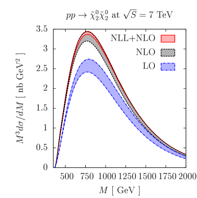
Refer to caption
Refer to caption
Refer to caption
Refer to caption
Figure 10: Same as Fig. 9 for the LHC with its current center-of-mass energy of S=7𝑆7\sqrt{S}=7 TeV.

current center-of-mass energy of S=7𝑆7\sqrt{S}=7 TeV and in Fig. 11 for

Refer to caption
Refer to caption
Refer to caption
Refer to caption
Figure 11: Same as Fig. 9 for the LHC with its design center-of-mass energy of S=14𝑆14\sqrt{S}=14 TeV.

the LHC with its design energy of S=14𝑆14\sqrt{S}=14 TeV. There are, however, two notable differences. First, the LHC is a pp𝑝𝑝pp collider, so that the cross section for χ~1+χ~20subscriptsuperscript~𝜒1subscriptsuperscript~𝜒02\tilde{\chi}^{+}_{1}\tilde{\chi}^{0}_{2} exceeds the one for χ~1χ~20subscriptsuperscript~𝜒1subscriptsuperscript~𝜒02\tilde{\chi}^{-}_{1}\tilde{\chi}^{0}_{2} by a factor of two and becomes even larger than the one for chargino pairs. Second, the NLO band is separated by a wider gap from the LO band than it was the case at Tevatron, whereas the NLL+NLO and NLO bands overlap considerably more. This is, of course, due to the fact that the light gauginos are now produced further away from the threshold of the 7 or 14 TeV collider, so that the importance of soft-gluon resummation is reduced. However, one still observes a sizeable reduction of the scale uncertainty from NLO to NLL+NLO.

Heavier gaugino pairs can only be produced with sizeable cross sections at the LHC. We therefore show in Figs. 12 and 13 the invariant mass
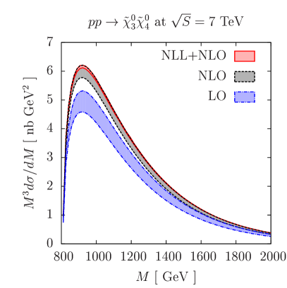
Refer to caption
Refer to caption
Refer to caption
Refer to caption
Figure 12: Same as Fig. 9 for the production of heavy gaugino pairs at the LHC with its current center-of-mass energy of S=7𝑆7\sqrt{S}=7 TeV.
Refer to caption
Refer to caption
Refer to caption
Refer to caption
Figure 13: Same as Fig. 9 for the production of heavy gaugino pairs at the LHC with its design center-of-mass energy of S=14𝑆14\sqrt{S}=14 TeV.

spectra M3dσ/dMsuperscript𝑀3d𝜎d𝑀M^{3}{\rm d}\sigma/{\rm d}M for the production of various combinations of χ~3,40subscriptsuperscript~𝜒034\tilde{\chi}^{0}_{3,4} and χ~2±subscriptsuperscript~𝜒plus-or-minus2\tilde{\chi}^{\pm}_{2} at the LHC with S=7𝑆7\sqrt{S}=7 TeV and 14 TeV and with mχ~30=400subscript𝑚subscriptsuperscript~𝜒03400m_{\tilde{\chi}^{0}_{3}}=400 GeV and mχ~2±mχ~40=415similar-to-or-equalssubscript𝑚subscriptsuperscript~𝜒plus-or-minus2subscript𝑚subscriptsuperscript~𝜒04415m_{\tilde{\chi}^{\pm}_{2}}\simeq m_{\tilde{\chi}^{0}_{4}}=415 GeV in the SPS1a’ scenario. The spectra start at M800830similar-to-or-equals𝑀800830M\simeq 800-830 GeV, and their magnitudes are considerably smaller than in the light gaugino case. However, they are now of comparable size for neutralino and chargino pairs due to the fact that the dominantly higgsino χ~30subscriptsuperscript~𝜒03\tilde{\chi}^{0}_{3} and χ~40subscriptsuperscript~𝜒04\tilde{\chi}^{0}_{4} now have sizeable couplings to the s𝑠s-channel Z𝑍Z-boson (see Tab. 1). The associated production of a neutralino and a chargino is again much larger for the positive chargino eigenstate than for its negative counterpart. The cross sections for χ~30χ~2±subscriptsuperscript~𝜒03subscriptsuperscript~𝜒plus-or-minus2\tilde{\chi}^{0}_{3}\tilde{\chi}^{\pm}_{2} pairs are very similar to those for χ~40χ~2±subscriptsuperscript~𝜒04subscriptsuperscript~𝜒plus-or-minus2\tilde{\chi}^{0}_{4}\tilde{\chi}^{\pm}_{2} pairs and therefore not shown. Higgsino-like neutralinos and charginos with large s𝑠s-channel contributions are produced as S𝑆S-waves, so that the invariant mass spectra rise more steeply at low M𝑀M than P𝑃P-wave produced gaugino-like neutralinos and charginos.

From Figs. 9-13, the impact of threshold resummation effects is difficult to estimate. We therefore present in Fig. 14 the relative
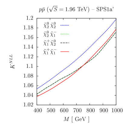
Refer to caption
Refer to caption
Refer to caption
Figure 14: Ratios KNLLsuperscript𝐾NLLK^{\rm NLL} of NLL+NLO over NLO differential cross sections as a function of the invariant mass M𝑀M of a light gaugino pair at the Tevatron (top left) and LHC with S=7𝑆7\sqrt{S}=7 TeV (top right) and S=14𝑆14\sqrt{S}=14 TeV (bottom) in the SPS1a’ scenario.

size

KNLL=dσNLL+NLOdσNLOsuperscript𝐾NLL𝑑superscript𝜎NLLNLO𝑑superscript𝜎NLOK^{\rm NLL}=\frac{d\sigma^{\rm NLL+NLO}}{d\sigma^{\rm NLO}} (102)

of the NLL+NLO prediction with respect to the NLO prediction. As one expects, the correction is larger at the Tevatron with its lower center-of-mass energy (top left) than at the LHC (top right and bottom) and increases with the invariant mass. The relatively small differences among the KNLLsuperscript𝐾NLLK^{\rm NLL}-factors for neutralino pair production and the channels involving at least one chargino can be traced to the fact that the former receives most of its contributions from t𝑡t- and u𝑢u-channel squark exchanges, which are more sensible to strong corrections than the exchanges of electroweak bosons in the s𝑠s-channel.

The KNLLsuperscript𝐾NLLK^{\rm NLL}-factors for the production of heavy gaugino pairs at the LHC with S=7𝑆7\sqrt{S}=7 TeV (14 TeV) are presented in Fig. 15 left (right).
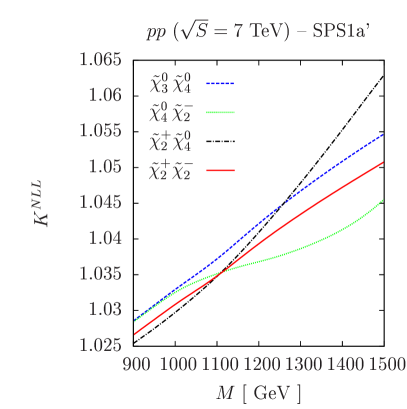
Refer to caption
Refer to caption
Figure 15: Same as Fig. 14 for heavy gaugino pairs at the LHC with S=7𝑆7\sqrt{S}=7 TeV (left) and S=14𝑆14\sqrt{S}=14 TeV (right).

They are larger than their counterparts for light gauginos in Fig. 14, since the gaugino masses as well as the invariant masses M𝑀M are now closer to the hadronic center-of-mass energies. In addition, the result for the χ~30χ~40subscriptsuperscript~𝜒03subscriptsuperscript~𝜒04\tilde{\chi}^{0}_{3}\tilde{\chi}^{0}_{4} channel differs no longer substantially from the other channels, since the heavy neutralinos are now higgsino-like and their production is now also dominated by the s𝑠s-channel exchange of a weak gauge boson.

IV.3 Total cross sections

The stability of the perturbative series and its reorganization is traditionally checked by varying the factorization and renormalization scales μFsubscript𝜇𝐹\mu_{F} and μRsubscript𝜇𝑅\mu_{R} about a central value μ0subscript𝜇0\mu_{0}. We therefore present now the total cross sections for the production of light gaugino pairs at the Tevatron (Fig. 16) and
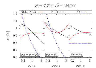
Refer to caption
Refer to caption
Refer to caption
Figure 16: Total cross sections for the production of neutralino (top left), chargino-neutralino (top right) and chargino pairs (bottom) at the Tevatron with S=1.96𝑆1.96\sqrt{S}=1.96 TeV in the LO (blue, dot-dashed), NLO (black, dashed) and NLL+NLO (red, full) approximation.

at the LHC with S=7𝑆7\sqrt{S}=7 TeV (Fig. 17) as a

Refer to caption
Refer to caption
Refer to caption
Refer to caption
Figure 17: Same as Fig. 16 for the LHC with its current center-of-mass energy of S=7𝑆7\sqrt{S}=7 TeV.

function of the ratio μF,R/μ0subscript𝜇𝐹𝑅subscript𝜇0\mu_{F,R}/\mu_{0}, where the central scale μ0subscript𝜇0\mu_{0} is now chosen to be the average mass of the produced gaugino pair. The LO prediction (blue, dot-dashed) of the electroweak processes under consideration is, of course, independent of the renormalization scale μRsubscript𝜇𝑅\mu_{R} (right part of the figures), whereas the NLO prediction (black, dashed) depends inversely on the logarithm of μRsubscript𝜇𝑅\mu_{R} through the strong coupling αs(μR)subscript𝛼𝑠subscript𝜇𝑅\alpha_{s}(\mu_{R}). At NLL accuracy (red, full), the resummed soft corrections attenuate this dependence and introduce a plateau region, so that the prediction is stabilized. The factorization scale μFsubscript𝜇𝐹\mu_{F} (central part of the figures) enters the hadronic cross section already at LO through the largely logarithmic dependence of the PDFs, which is then attenuated by the factorization of initial-state singularities at NLO and further at NLL accuracy. In all cases, the resulting total NLL+NLO prediction is thus much less dependent on the common scale μF=μR=μsubscript𝜇𝐹subscript𝜇𝑅𝜇\mu_{F}=\mu_{R}=\mu (left part of the figures) than the LO and NLO estimates.

In Tab. 3 we present the total cross sections for the trilepton

Table 3: Total cross sections for the production of χ~1+χ~20superscriptsubscript~𝜒1superscriptsubscript~𝜒20\tilde{\chi}_{1}^{+}\tilde{\chi}_{2}^{0} pairs in the SPS1a’ scenario at different hadron colliders and center-of-mass energies in the LO, NLO and NLL+NLO approximation, together with the corresponding scale and PDF uncertainties.
Colliders σNLL+NLOsuperscript𝜎NLLNLO\sigma^{\rm NLL+NLO} [fb] σNLOsuperscript𝜎NLO\sigma^{\rm NLO} [fb] σLOsuperscript𝜎LO\sigma^{\rm LO} [fb]
pp¯𝑝¯𝑝p\bar{p}(S=1.96𝑆1.96\sqrt{S}=1.96 TeV) 30.90.2+0.11.9+1.530.9^{+0.1}_{-0.2}\;{}^{+1.5}_{-1.9} 31.21.2+0.91.9+1.531.2^{+0.9}_{-1.2}\;{}^{+1.5}_{-1.9} 27.23.0+3.6subscriptsuperscript27.23.63.027.2^{+3.6}_{-3.0}
pp𝑝𝑝pp(S=7𝑆7\sqrt{S}=7 TeV) 263.31.3+0.613.2+11.4263.3^{+0.6}_{-1.3}\;{}^{+11.4}_{-13.2} 265.54.3+5.013.2+11.5265.5^{+5.0}_{-4.3}\;{}^{+11.5}_{-13.2} 223.17.1+6.9subscriptsuperscript223.16.97.1223.1^{+6.9}_{-7.1}
pp𝑝𝑝pp(S=10𝑆10\sqrt{S}=10 TeV) 470.72.3+1.419.3+17.7470.7^{+1.4}_{-2.3}\;{}^{+17.7}_{-19.3} 474.06.0+8.319.4+17.7474.0^{+8.3}_{-6.0}\;{}^{+17.7}_{-19.4} 387.44.3+2.5subscriptsuperscript387.42.54.3387.4^{+2.5}_{-4.3}
pp𝑝𝑝pp(S=14𝑆14\sqrt{S}=14 TeV) 772.73.1+1.626.7+25.5772.7^{+1.6}_{-3.1}\;{}^{+25.5}_{-26.7} 777.57.4+11.926.7+25.5777.5^{+11.9}_{-7.4}\;{}^{+25.5}_{-26.7} 623.79.3+4.7subscriptsuperscript623.74.79.3623.7^{+4.7}_{-9.3}

channel in the SPS1a’ scenario at the Tevatron (S=1.96𝑆1.96\sqrt{S}=1.96 TeV) and LHC (S=7𝑆7\sqrt{S}=7, 10 and 14 TeV). Besides the central values (in fb) at LO, NLO and NLL+NLO, we also present the scale and PDF uncertainties. The former are estimated as described above by a common variation of the renormalization and factorization scales by a factor of two about the average mass of the two gauginos, the latter through

ΔσPDF+=i=122[max(σ+iσ0,σiσ0,0)]2Δsubscript𝜎limit-fromPDFsuperscriptsubscript𝑖122superscriptdelimited-[]subscript𝜎𝑖subscript𝜎0subscript𝜎𝑖subscript𝜎002\displaystyle\Delta\sigma_{\rm PDF+}~{}=~{}\sqrt{\sum_{i=1}^{22}\left[\max\left(\sigma_{+i}-\sigma_{0},\sigma_{-i}-\sigma_{0},0\right)\right]^{2}} , ΔσPDF=i=122[max(σ0σ+i,σ0σi,0)]2Δsubscript𝜎limit-fromPDFsuperscriptsubscript𝑖122superscriptdelimited-[]subscript𝜎0subscript𝜎𝑖subscript𝜎0subscript𝜎𝑖02\displaystyle\Delta\sigma_{\rm PDF-}~{}=~{}\sqrt{\sum_{i=1}^{22}\left[\max\left(\sigma_{0}-\sigma_{+i},\sigma_{0}-\sigma_{-i},0\right)\right]^{2}} (103)

along the 22 eigenvector directions defined by the CTEQ collaboration. Since these are available only for the NLO fit CTEQ6.6M, but not for the LO fit CTEQ6.6L1, we do not present a PDF uncertainty for the LO prediction. Furthermore, the same PDF set enters at NLO and NLL+NLO, so that the PDF uncertainties for these two predictions coincide. The most important result is again the considerable reduction of the scale uncertainty from LO to NLO and then to NLL+NLO. The total cross sections increase with the available center-of-mass energy due to the higher parton luminosity at smaller values of x𝑥x. A crude estimate gives

σppsubscript𝜎𝑝𝑝\displaystyle\sigma_{pp} =\displaystyle= m2/S1dτfq/p(xq)fq¯/p(xq¯)σqq¯m2/S1dττ1.81τS,S1.6\displaystyle\int_{m^{2}/S}^{1}{\rm d}\tau\,f_{q/p}(x_{q})\,f_{\bar{q}/p}(x_{\bar{q}})\,\sigma_{q\bar{q}}~{}\sim~{}\int_{m^{2}/S}^{1}{\rm d}\tau\,\tau^{-1.8}{1\over\tau S},~{}\sim~{}\sqrt{S}^{1.6} (104)

which agrees with the cross sections given in Tab. 3 surprisingly well.

In Tab. 4 we fix the LHC center-of-mass energy to its design value

Table 4: Total cross sections for the production of various gaugino pairs in the SPS1a’ scenario at the LHC with its design center-of-mass energy of S=14𝑆14\sqrt{S}=14 TeV. The central predictions are given at LO, NLO and NLL+NLO together with the corresponding scale and PDF uncertainties.
Gaugino pair σNLL+NLOsuperscript𝜎NLLNLO\sigma^{\rm NLL+NLO} [fb] σNLOsuperscript𝜎NLO\sigma^{\rm NLO} [fb] σLOsuperscript𝜎LO\sigma^{\rm LO} [fb]
χ~20χ~20superscriptsubscript~𝜒20superscriptsubscript~𝜒20\tilde{\chi}_{2}^{0}\tilde{\chi}_{2}^{0} 25.10.2+0.30.7+1.225.1^{+0.3}_{-0.2}\;{}^{+1.2}_{-0.7} 25.50.6+0.80.7+1.325.5^{+0.8}_{-0.6}\;{}^{+1.3}_{-0.7} 19.20.4+0.3subscriptsuperscript19.20.30.419.2^{+0.3}_{-0.4}
χ~1+χ~1superscriptsubscript~𝜒1superscriptsubscript~𝜒1\tilde{\chi}_{1}^{+}\tilde{\chi}_{1}^{-} 665.82.2+1.020.6+20.6665.8^{+1.0}_{-2.2}\;{}^{+20.6}_{-20.6} 671.16.6+10.820.6+20.7671.1^{+10.8}_{-6.6}\;{}^{+20.7}_{-20.6} 533.47.3+3.4subscriptsuperscript533.43.47.3533.4^{+3.4}_{-7.3}
χ~20χ~1superscriptsubscript~𝜒20superscriptsubscript~𝜒1\tilde{\chi}_{2}^{0}\tilde{\chi}_{1}^{-} 433.30.8+0.616.0+17.9433.3^{+0.6}_{-0.8}\;{}^{+17.9}_{-16.0} 436.93.5+7.216.1+17.9436.9^{+7.2}_{-3.5}\;{}^{+17.9}_{-16.1} 348.34.9+2.2subscriptsuperscript348.32.24.9348.3^{+2.2}_{-4.9}
χ~1+χ~20superscriptsubscript~𝜒1superscriptsubscript~𝜒20\tilde{\chi}_{1}^{+}\tilde{\chi}_{2}^{0} 772.73.1+1.626.7+25.5772.7^{+1.6}_{-3.1}\;{}^{+25.5}_{-26.7} 777.57.4+11.926.7+25.5777.5^{+11.9}_{-7.4}\;{}^{+25.5}_{-26.7} 623.79.3+4.7subscriptsuperscript623.74.79.3623.7^{+4.7}_{-9.3}
χ~30χ~40superscriptsubscript~𝜒30superscriptsubscript~𝜒40\tilde{\chi}_{3}^{0}\tilde{\chi}_{4}^{0} 14.60.1+0.00.7+0.714.6^{+0.0}_{-0.1}\;{}^{+0.7}_{-0.7} 14.80.3+0.30.7+0.714.8^{+0.3}_{-0.3}\;{}^{+0.7}_{-0.7} 12.10.5+0.5subscriptsuperscript12.10.50.512.1^{+0.5}_{-0.5}
χ~2+χ~2superscriptsubscript~𝜒2superscriptsubscript~𝜒2\tilde{\chi}_{2}^{+}\tilde{\chi}_{2}^{-} 14.00.0+0.10.6+0.714.0^{+0.1}_{-0.0}\;{}^{+0.7}_{-0.6} 14.20.3+0.30.6+0.714.2^{+0.3}_{-0.3}\;{}^{+0.7}_{-0.6} 11.70.5+0.5subscriptsuperscript11.70.50.511.7^{+0.5}_{-0.5}
χ~30χ~2superscriptsubscript~𝜒30superscriptsubscript~𝜒2\tilde{\chi}_{3}^{0}\tilde{\chi}_{2}^{-} 8.50.0+0.00.5+0.68.5^{+0.0}_{-0.0}\;{}^{+0.6}_{-0.5} 8.60.2+0.20.5+0.68.6^{+0.2}_{-0.2}\;{}^{+0.6}_{-0.5} 6.90.3+0.3subscriptsuperscript6.90.30.36.9^{+0.3}_{-0.3}
χ~2+χ~30superscriptsubscript~𝜒2superscriptsubscript~𝜒30\tilde{\chi}_{2}^{+}\tilde{\chi}_{3}^{0} 19.10.1+0.11.0+0.919.1^{+0.1}_{-0.1}\;{}^{+0.9}_{-1.0} 19.30.4+0.41.0+0.919.3^{+0.4}_{-0.4}\;{}^{+0.9}_{-1.0} 16.00.7+0.7subscriptsuperscript16.00.70.716.0^{+0.7}_{-0.7}
χ~40χ~2superscriptsubscript~𝜒40superscriptsubscript~𝜒2\tilde{\chi}_{4}^{0}\tilde{\chi}_{2}^{-} 7.80.0+0.00.5+0.57.8^{+0.0}_{-0.0}\;{}^{+0.5}_{-0.5} 7.90.2+0.20.5+0.57.9^{+0.2}_{-0.2}\;{}^{+0.5}_{-0.5} 6.40.3+0.3subscriptsuperscript6.40.30.36.4^{+0.3}_{-0.3}
χ~2+χ~40superscriptsubscript~𝜒2superscriptsubscript~𝜒40\tilde{\chi}_{2}^{+}\tilde{\chi}_{4}^{0} 17.70.1+0.10.9+0.817.7^{+0.1}_{-0.1}\;{}^{+0.8}_{-0.9} 17.80.3+0.40.9+0.817.8^{+0.4}_{-0.3}\;{}^{+0.8}_{-0.9} 14.90.6+0.7subscriptsuperscript14.90.70.614.9^{+0.7}_{-0.6}

of S=14𝑆14\sqrt{S}=14 TeV and show the total production cross sections for light and heavy gaugino pairs in LO, NLO and NLL+NLO together with the corresponding theoretical uncertainties. As it was already mentioned above, the cross section for the higgsino-like χ~30χ~40subscriptsuperscript~𝜒03subscriptsuperscript~𝜒04\tilde{\chi}^{0}_{3}\tilde{\chi}^{0}_{4} pairs is about as large as the one for χ~2+χ~2superscriptsubscript~𝜒2superscriptsubscript~𝜒2\tilde{\chi}_{2}^{+}\tilde{\chi}_{2}^{-} pairs, and it is in fact not much smaller than the one for the considerably lighter gaugino-like χ~20χ~20subscriptsuperscript~𝜒02subscriptsuperscript~𝜒02\tilde{\chi}^{0}_{2}\tilde{\chi}^{0}_{2} pairs. In general, the heavy gaugino cross sections are, however, significantly smaller than those for light gauginos.

In Tab. 5, we present finally total cross sections for the trilepton

Table 5: Total cross sections for the production of χ~1+χ~20superscriptsubscript~𝜒1superscriptsubscript~𝜒20\tilde{\chi}_{1}^{+}\tilde{\chi}_{2}^{0} pairs at the LHC with its current center-of-mass energy of S=7𝑆7\sqrt{S}=7 TeV for different SUSY benchmark points. The central predictions are given at LO, NLO and NLL+NLO together with the corresponding scale and PDF uncertainties.
Scenario σNLL+NLOsuperscript𝜎NLLNLO\sigma^{\rm NLL+NLO} [fb] σNLOsuperscript𝜎NLO\sigma^{\rm NLO} [fb] σLOsuperscript𝜎LO\sigma^{\rm LO} [fb]
LM1 294.61.4+0.814.5+12.8294.6^{+0.8}_{-1.4}\;{}^{+12.8}_{-14.5} 297.04.8+5.814.5+12.8297.0^{+5.8}_{-4.8}\;{}^{+12.8}_{-14.5} 248.27.5+7.1subscriptsuperscript248.27.17.5248.2^{+7.1}_{-7.5}
LM7 538.93.5+2.426.7+23.9538.9^{+2.4}_{-3.5}\;{}^{+23.9}_{-26.7} 543.810.7+12.826.8+24.0543.8^{+12.8}_{-10.7}\;{}^{+24.0}_{-26.8} 441.214.3+14.0subscriptsuperscript441.214.014.3441.2^{+14.0}_{-14.3}
LM9 1736.212.1+8.074.3+68.81736.2^{+8.0}_{-12.1}\;{}^{+68.8}_{-74.3} 1750.328.8+38.874.4+69.01750.3^{+38.8}_{-28.8}\;{}^{+69.0}_{-74.4} 1374.415.7+8.4subscriptsuperscript1374.48.415.71374.4^{+8.4}_{-15.7}
SU2 171.70.9+0.59.8+8.5171.7^{+0.5}_{-0.9}\;{}^{+8.5}_{-9.8} 173.43.9+4.29.8+8.5173.4^{+4.2}_{-3.9}\;{}^{+8.5}_{-9.8} 145.07.0+7.4subscriptsuperscript145.07.47.0145.0^{+7.4}_{-7.0}
SU3 116.90.4+0.16.4+5.6116.9^{+0.1}_{-0.4}\;{}^{+5.6}_{-6.4} 118.02.1+2.26.4+5.6118.0^{+2.2}_{-2.1}\;{}^{+5.6}_{-6.4} 101.64.4+4.6subscriptsuperscript101.64.64.4101.6^{+4.6}_{-4.4}
SU2+JV 170.40.7+0.29.8+8.6170.4^{+0.2}_{-0.7}\;{}^{+8.6}_{-9.8} 172.03.6+3.99.9+8.6172.0^{+3.9}_{-3.6}\;{}^{+8.6}_{-9.9} 145.07.0+7.4subscriptsuperscript145.07.47.0145.0^{+7.4}_{-7.0}
SU3+JV 115.40.1+0.16.4+5.6115.4^{+0.1}_{-0.1}\;{}^{+5.6}_{-6.4} 116.61.8+1.96.4+5.6116.6^{+1.9}_{-1.8}\;{}^{+5.6}_{-6.4} 101.64.4+4.6subscriptsuperscript101.64.64.4101.6^{+4.6}_{-4.4}

channel in our different benchmark scenarios at the LHC with its current center-of-mass energy of S=7𝑆7\sqrt{S}=7 TeV. Since the masses of χ~1±subscriptsuperscript~𝜒plus-or-minus1\tilde{\chi}^{\pm}_{1} and χ~20subscriptsuperscript~𝜒02\tilde{\chi}^{0}_{2} are always rather similar, one expects also similar total cross sections. This is indeed confirmed by the S=7𝑆7\sqrt{S}=7 TeV results in Tab. 3 and the numbers in Tab. 5 with the notable exceptions of LM7 and LM9, where the cross section is about a factor of two and one order of magnitude larger than for the other points, respectively. This is partly due to the lower gaugino masses at LM9 and partly to the much heavier squark masses, which suppress the t𝑡t- and u𝑢u-channels and thus their destructive interference with the s𝑠s-channel amplitudes. The additional jet veto (JV), i.e. the rejection of events containing jets with transverse momentum pT>20subscript𝑝𝑇20p_{T}>20 GeV, envisaged by the ATLAS collaboration to suppress the background from top quark pair production, has obviously no consequences at LO, since gauginos are exclusively produced at this order. An additional quark or gluon can only be present at NLO or NLL+NLO, and restricting its transverse momentum to low values reduces the total cross sections slightly with respect to the unrestricted predictions. The small reduction of the signal cross section in combination with a large reduction of the background should therefore indeed lead to a much better significance.

V Conclusions

In summary, we presented in this paper a complete analysis of threshold resummation effects on direct light and heavy gaugino pair production at the Tevatron and at the LHC with its current, intermediate, and design center-of-mass energies. We confirmed the existing NLO calculation and extended it to include also mixing effects for intermediate squarks. Soft gluon radiation in the threshold region was resummed at leading and next-to-leading logarithmic accuracy into a Sudakov exponential, and the full SUSY-QCD corrections were retained in the finite coefficient function. This allowed us to correctly match the resummed cross section at NLL accuracy to the NLO perturbative cross section. Universal subleading logarithms coming from the splitting of initial partons were resummed in full matrix form, i.e. including also non-diagonal splittings. We found that resummation increased the invariant mass spectra and total cross sections only slightly, but stabilized the reorganized perturbative series considerably with respect to the fixed-order calculation. For future reference, we presented total cross sections with the corresponding theoretical errors from scale and PDF variations at LO, NLO and NLL+NLO in tabular form for several commonly used SUSY benchmark points, light and heavy gaugino pairs, and various hadron collider types and energies.

Appendix A Quark and squark couplings to weak gauge bosons and gauginos

The coupling strengths of the electroweak gauge bosons Z𝑍Z and W𝑊W to left- and right-handed (s)quarks q𝑞q (q~~𝑞\tilde{q}) with weak isospin Tq3subscriptsuperscript𝑇3𝑞T^{3}_{q} and fractional electric charge eqsubscript𝑒𝑞e_{q} are given by

{LqqZ,RqqZ}subscript𝐿𝑞𝑞𝑍subscript𝑅𝑞𝑞𝑍\displaystyle\{L_{qqZ},R_{qqZ}\} =\displaystyle= 12cW(Tq3eqxW),12subscript𝑐𝑊subscriptsuperscript𝑇3𝑞subscript𝑒𝑞subscript𝑥𝑊\displaystyle\ -\frac{1}{2c_{W}}(T^{3}_{q}-e_{q}\,x_{W})\ ,
{Lq~iq~jZ,Rq~iq~jZ}subscript𝐿subscript~𝑞𝑖subscript~𝑞𝑗𝑍subscript𝑅subscript~𝑞𝑖subscript~𝑞𝑗𝑍\displaystyle\{L_{\tilde{q}_{i}\tilde{q}_{j}Z},R_{\tilde{q}_{i}\tilde{q}_{j}Z}\} =\displaystyle= 12cW(Tq3eqxW){Ri1q~Rj1q~,Ri2q~Rj2q~},12subscript𝑐𝑊subscriptsuperscript𝑇3𝑞subscript𝑒𝑞subscript𝑥𝑊subscriptsuperscript𝑅~𝑞𝑖1subscriptsuperscript𝑅~𝑞𝑗1subscriptsuperscript𝑅~𝑞𝑖2subscriptsuperscript𝑅~𝑞𝑗2\displaystyle\ -\frac{1}{2c_{W}}(T^{3}_{q}-e_{q}\,x_{W})\{R^{\tilde{q}}_{i1}\,R^{\tilde{q}\ast}_{j1},R^{\tilde{q}}_{i2}\,R^{\tilde{q}\ast}_{j2}\}\ ,
{LudW,RudW}subscript𝐿𝑢𝑑𝑊subscript𝑅𝑢𝑑𝑊\displaystyle\{L_{udW},R_{udW}\} =\displaystyle= {Vud2cW,0},subscript𝑉𝑢𝑑2subscript𝑐𝑊0\displaystyle\ \{-{V_{ud}\over 2c_{W}},0\}\ ,
{Lu~id~jW,Ru~id~jW}subscript𝐿subscript~𝑢𝑖subscript~𝑑𝑗𝑊subscript𝑅subscript~𝑢𝑖subscript~𝑑𝑗𝑊\displaystyle\{L_{\tilde{u}_{i}\tilde{d}_{j}W},R_{\tilde{u}_{i}\tilde{d}_{j}W}\} =\displaystyle= {Vud2cWRi1u~Rj1d~, 0},subscript𝑉𝑢𝑑2subscript𝑐𝑊subscriptsuperscript𝑅~𝑢𝑖1subscriptsuperscript𝑅~𝑑𝑗1 0\displaystyle\ \{-\frac{V_{ud}}{2c_{W}}R^{\tilde{u}}_{i1}\,R^{\tilde{d}\ast}_{j1},\,0\}, (105)

where xW=1cW2=sW2=sin2θWsubscript𝑥𝑊1superscriptsubscript𝑐𝑊2superscriptsubscript𝑠𝑊2superscript2subscript𝜃𝑊x_{W}=1-c_{W}^{2}=s_{W}^{2}=\sin^{2}\theta_{W} is the squared sine of the electroweak mixing angle, Riju~,d~subscriptsuperscript𝑅~𝑢~𝑑𝑖𝑗R^{\tilde{u},\tilde{d}}_{ij} are the elements of the rotation matrices diagonalizing the up- and down-type squark mass matrices, and Vudsubscript𝑉𝑢𝑑V_{ud} are the elements of the CKM matrix. Their SUSY counterparts, i.e. the squark-quark-gaugino couplings, are given by

Ld~jdχ~i0subscript𝐿subscript~𝑑𝑗𝑑subscriptsuperscript~𝜒0𝑖\displaystyle L_{\tilde{d}_{j}d\tilde{\chi}^{0}_{i}} =\displaystyle= (edTd3)sWNi1+Tq3cWNi22cWRj1d~+mdNi322mWcosβRj2d~,subscript𝑒𝑑subscriptsuperscript𝑇3𝑑subscript𝑠𝑊subscript𝑁𝑖1subscriptsuperscript𝑇3𝑞subscript𝑐𝑊subscript𝑁𝑖22subscript𝑐𝑊subscriptsuperscript𝑅~𝑑𝑗1subscript𝑚𝑑subscript𝑁𝑖322subscript𝑚𝑊𝛽subscriptsuperscript𝑅~𝑑𝑗2\displaystyle\ \frac{(e_{d}-T^{3}_{d})\,s_{W}\,N_{i1}+T^{3}_{q}\,c_{W}\,N_{i2}}{\sqrt{2}\,c_{W}}R^{\tilde{d}\ast}_{j1}+\frac{m_{d}\,N_{i3}}{2\sqrt{2}\,m_{W}\,\cos\beta}R^{\tilde{d}\ast}_{j2}\ ,~{}
Rd~jdχ~i0subscript𝑅subscript~𝑑𝑗𝑑superscriptsubscript~𝜒𝑖0\displaystyle R_{\tilde{d}_{j}d\tilde{\chi}_{i}^{0}} =\displaystyle= edsWNi12cWRj2d~+mdNi322mWcosβRj1d~,subscript𝑒𝑑subscript𝑠𝑊subscriptsuperscript𝑁𝑖12subscript𝑐𝑊subscriptsuperscript𝑅~𝑑𝑗2subscript𝑚𝑑subscriptsuperscript𝑁𝑖322subscript𝑚𝑊𝛽subscriptsuperscript𝑅~𝑑𝑗1\displaystyle\ -\frac{e_{d}\,s_{W}\,N^{\ast}_{i1}}{\sqrt{2}\,c_{W}}R^{\tilde{d}\ast}_{j2}+\frac{m_{d}\,N^{\ast}_{i3}}{2\sqrt{2}\,m_{W}\,\cos\beta}R^{\tilde{d}\ast}_{j1}\ ,~{}
Lu~juχ~i0subscript𝐿subscript~𝑢𝑗𝑢subscriptsuperscript~𝜒0𝑖\displaystyle L_{\tilde{u}_{j}u\tilde{\chi}^{0}_{i}} =\displaystyle= (euTu3)sWNi1+Tq3cWNi22cWRj1u~+muNi422mWsinβRj2u~,subscript𝑒𝑢subscriptsuperscript𝑇3𝑢subscript𝑠𝑊subscript𝑁𝑖1subscriptsuperscript𝑇3𝑞subscript𝑐𝑊subscript𝑁𝑖22subscript𝑐𝑊subscriptsuperscript𝑅~𝑢𝑗1subscript𝑚𝑢subscript𝑁𝑖422subscript𝑚𝑊𝛽subscriptsuperscript𝑅~𝑢𝑗2\displaystyle\ \frac{(e_{u}-T^{3}_{u})\,s_{W}\,N_{i1}+T^{3}_{q}\,c_{W}\,N_{i2}}{\sqrt{2}\,c_{W}}R^{\tilde{u}\ast}_{j1}+\frac{m_{u}\,N_{i4}}{2\sqrt{2}\,m_{W}\,\sin\beta}R^{\tilde{u}\ast}_{j2}\ ,~{}
Ru~juχ~i0subscript𝑅subscript~𝑢𝑗𝑢superscriptsubscript~𝜒𝑖0\displaystyle R_{\tilde{u}_{j}u\tilde{\chi}_{i}^{0}} =\displaystyle= eusWNi12cWRj2u~+muNi422mWsinβRj1u~,subscript𝑒𝑢subscript𝑠𝑊superscriptsubscript𝑁𝑖12subscript𝑐𝑊subscriptsuperscript𝑅~𝑢𝑗2subscript𝑚𝑢superscriptsubscript𝑁𝑖422subscript𝑚𝑊𝛽subscriptsuperscript𝑅~𝑢𝑗1\displaystyle\ -\frac{e_{u}\,s_{W}\,N_{i1}^{\ast}}{\sqrt{2}c_{W}}R^{\tilde{u}\ast}_{j2}+\frac{m_{u}\,N_{i4}^{\ast}}{2\sqrt{2}\,m_{W}\,\sin\beta}R^{\tilde{u}\ast}_{j1}\ ,~{}
Ld~juχ~i±subscript𝐿subscript~𝑑𝑗𝑢superscriptsubscript~𝜒𝑖plus-or-minus\displaystyle L_{\tilde{d}_{j}u\tilde{\chi}_{i}^{\pm}} =\displaystyle= 12[Ui1Rj1d~mdUi22mWcosβRj2d~]Vud,12delimited-[]subscript𝑈𝑖1subscriptsuperscript𝑅~𝑑𝑗1subscript𝑚𝑑subscript𝑈𝑖22subscript𝑚𝑊𝛽subscriptsuperscript𝑅~𝑑𝑗2subscript𝑉𝑢𝑑\displaystyle\ \frac{1}{2}\bigg{[}U_{i1}\,R^{\tilde{d}\ast}_{j1}-\frac{m_{d}\,U_{i2}}{\sqrt{2}\,m_{W}\,\cos\beta}R^{\tilde{d}\ast}_{j2}\bigg{]}V_{ud}\ ,~{}
Rd~juχ~i±subscript𝑅subscript~𝑑𝑗𝑢superscriptsubscript~𝜒𝑖plus-or-minus\displaystyle R_{\tilde{d}_{j}u\tilde{\chi}_{i}^{\pm}} =\displaystyle= muVi2Vud22mWsinβRj1d~,subscript𝑚𝑢superscriptsubscript𝑉𝑖2subscript𝑉𝑢𝑑22subscript𝑚𝑊𝛽subscriptsuperscript𝑅~𝑑𝑗1\displaystyle\ -\frac{m_{u}\,V_{i2}^{\ast}\,V_{ud}}{2\sqrt{2}\,m_{W}\,\sin\beta}R^{\tilde{d}\ast}_{j1}\ ,~{}
Lu~jdχ~i±subscript𝐿subscript~𝑢𝑗𝑑superscriptsubscript~𝜒𝑖plus-or-minus\displaystyle L_{\tilde{u}_{j}d\tilde{\chi}_{i}^{\pm}} =\displaystyle= 12[Vi1Rj1u~muVi22mWsinβRj2u~]Vud,12delimited-[]subscript𝑉𝑖1subscriptsuperscript𝑅~𝑢𝑗1subscript𝑚𝑢subscript𝑉𝑖22subscript𝑚𝑊𝛽subscriptsuperscript𝑅~𝑢𝑗2superscriptsubscript𝑉𝑢𝑑\displaystyle\ \frac{1}{2}\bigg{[}V_{i1}\,R^{\tilde{u}\ast}_{j1}-\frac{m_{u}\,V_{i2}}{\sqrt{2}\,m_{W}\,\sin\beta}R^{\tilde{u}\ast}_{j2}\bigg{]}V_{ud}^{\ast}\ ,~{}
Ru~jdχ~i±subscript𝑅subscript~𝑢𝑗𝑑superscriptsubscript~𝜒𝑖plus-or-minus\displaystyle R_{\tilde{u}_{j}d\tilde{\chi}_{i}^{\pm}} =\displaystyle= mdUi2Vud22mWcosβRj1u~,subscript𝑚𝑑subscriptsuperscript𝑈𝑖2subscriptsuperscript𝑉𝑢𝑑22subscript𝑚𝑊𝛽subscriptsuperscript𝑅~𝑢𝑗1\displaystyle\ -\frac{m_{d}\,U^{\ast}_{i2}V^{\ast}_{ud}}{2\sqrt{2}\,m_{W}\,\cos\beta}R^{\tilde{u}\ast}_{j1}~{}, (106)

where the matrices N𝑁N, U𝑈U and V𝑉V diagonalize the neutral and charged gaugino-higgsino mass matrices, mu,dsubscript𝑚𝑢𝑑m_{u,d} are the up- and down-type quark masses, and mWsubscript𝑚𝑊m_{W} is the mass of the W𝑊W-boson. All other couplings vanish due to electromagnetic charge conservation Nilles:1983ge .

Acknowledgements.
This work has been supported by a Ph.D. fellowship of the French ministry for education and research and by the Theory-LHC-France initiative of the CNRS/IN2P3.

References

  • (1) H. P. Nilles, Phys. Rept.  110 (1984) 1; H. E. Haber and G. L. Kane, Phys. Rept.  117 (1985) 75; J. F. Gunion and H. E. Haber, Nucl. Phys.  B 272 (1986) 1 [Erratum-ibid.  B 402 (1993) 567].
  • (2) E. Witten, Nucl. Phys.  B 188 (1981) 513.
  • (3) S. Dimopoulos, S. Raby and F. Wilczek, Phys. Rev.  D 24 (1981) 1681.
  • (4) J. R. Ellis, J. S. Hagelin, D. V. Nanopoulos, K. A. Olive and M. Srednicki, Nucl. Phys.  B 238 (1984) 453.
  • (5) V. Barger, R. Robinett, W. Keung and R. Phillips, Phys. Lett.  B 131 (1983) 372; S. Dawson, E. Eichten and C. Quigg, Phys. Rev.  D 31 (1985) 1581; D. A. Dicus, S. Nandi and J. Woodside, Phys. Rev.  D 41 (1990) 2347; M. Klasen and G. Pignol, Phys. Rev.  D 75 (2007) 115003.
  • (6) G. Bozzi, B. Fuks and M. Klasen, Phys. Rev.  D 72 (2005) 035016; D. Berdine and D. Rainwater, Phys. Rev.  D 72 (2005) 075003; S. Bornhauser, M. Drees, H. K. Dreiner and J. S. Kim, Phys. Rev.  D 76 (2007) 095020.
  • (7) T. Gehrmann, D. Maitre and D. Wyler, Nucl. Phys.  B 703 (2004) 147; G. Bozzi, B. Fuks and M. Klasen, Phys. Lett.  B 609 (2005) 339; J. Debove, B. Fuks and M. Klasen, Phys. Rev.  D 78 (2008) 074020.
  • (8) G. Bozzi, B. Fuks, B. Herrmann and M. Klasen, Nucl. Phys.  B 787 (2007) 1; F. del Aguila et al., Eur. Phys. J.  C 57 (2008) 183; B. Fuks, B. Herrmann and M. Klasen, Nucl. Phys.  B 810 (2009) 266.
  • (9) A. T. Alan, K. Cankoçak and D. A. Demir, Phys. Rev.  D 75 (2007) 095002 [Erratum-ibid.  D 76 (2007) 119903].
  • (10) W. Beenakker, R. Höpker, M. Spira and P. M. Zerwas, Nucl. Phys.  B 492 (1997) 51; W. Beenakker, M. Krämer, T. Plehn, M. Spira and P. M. Zerwas, Nucl. Phys.  B 515 (1998) 3; H. Baer, B. W. Harris and M. H. Reno, Phys. Rev.  D 57 (1998) 5871; E. L. Berger, M. Klasen and T. M. P. Tait, Phys. Rev.  D 59 (1999) 074024; E. L. Berger, M. Klasen and T. M. P. Tait, Phys. Lett.  B 459 (1999) 165; E. L. Berger, M. Klasen and T. M. P. Tait, Phys. Rev.  D 62 (2000) 095014 [Erratum-ibid.  67 (2003) 099901]; M. Spira, arXiv:hep-ph/0211145; L. G. Jin, C. S. Li and J. J. Liu, Eur. Phys. J.  C 30 (2003) 77; L. G. Jin, C. S. Li and J. J. Liu, Phys. Lett.  B 561 (2003) 135.
  • (11) W. Beenakker, M. Klasen, M. Krämer, T. Plehn, M. Spira and P. M. Zerwas, Phys. Rev. Lett.  83 (1999) 3780 [Erratum-ibid.  100 (2008) 029901].
  • (12) W. Hollik, M. Kollar and M. K. Trenkel, JHEP 0802 (2008) 018; W. Hollik, E. Mirabella and M. K. Trenkel, JHEP 0902 (2009) 002; E. Mirabella, JHEP 0912 (2009) 012.
  • (13) G. Bozzi, B. Fuks and M. Klasen, Phys. Rev.  D 74 (2006) 015001; M. Klasen, Nucl. Phys. Proc. Suppl.  160 (2006) 111; L. L. Yang, C. S. Li, J. J. Liu and Q. Li, Phys. Rev.  D 72 (2005) 074026; H. K. Dreiner, S. Grab, M. Krämer and M. K. Trenkel, Phys. Rev.  D 75 (2007) 035003; Y. Q. Chen, T. Han and Z. G. Si, JHEP 0705 (2007) 068; J. Debove, B. Fuks and M. Klasen, Phys. Lett.  B 688 (2010) 208; J. Debove, arXiv:0908.4149 [hep-ph].
  • (14) G. Bozzi, B. Fuks and M. Klasen, Nucl. Phys.  B 777 (2007) 157; A. Kulesza and L. Motyka, Phys. Rev. Lett.  102 (2009) 111802; U. Langenfeld and S. O. Moch, Phys. Lett.  B 675 (2009) 210; A. Kulesza and L. Motyka, Phys. Rev.  D 80 (2009) 095004; W. Beenakker, S. Brensing, M. Krämer, A. Kulesza, E. Laenen and I. Niessen, JHEP 0912 (2009) 041.
  • (15) G. Bozzi, B. Fuks and M. Klasen, Nucl. Phys.  B 794 (2008) 46; B. Fuks, M. Klasen, F. Ledroit, Q. Li and J. Morel, Nucl. Phys.  B 797 (2008) 322.
  • (16) T. Aaltonen et al. [CDF Collaboration], Phys. Rev. Lett.  101 (2008) 251801; R. Forrest [CDF Collaboration], arXiv:0910.1931 [hep-ex]; V. M. Abazov et al. [D0 Collaboration], Phys. Lett.  B 680 (2009) 34.
  • (17) C. S. Li, Z. Li, R. J. Oakes and L. L. Yang, Phys. Rev.  D 77 (2008) 034010.
  • (18) G. Passarino and M. J. G. Veltman, Nucl. Phys.  B 160 (1979) 151.
  • (19) M. Böhm, A. Denner and H. Joos, Gauge theories of the strong and electroweak interaction. Teubner, Stuttgart (2001).
  • (20) J. A. Aguilar-Saavedra et al., Eur. Phys. J.  C 46 (2006) 43.
  • (21) S. Catani and M. H. Seymour, Nucl. Phys.  B 485 (1997) 291 [Erratum-ibid.  B 510 (1998) 503].
  • (22) G. Sterman, Nucl. Phys.  B 281 (1987) 310; N. Kidonakis and G. Sterman, Nucl. Phys.  B 505 (1997) 321; N. Kidonakis, G. Oderda and G. Sterman, Nucl. Phys.  B 525 (1998) 299.
  • (23) G. Altarelli and G. Parisi, Nucl. Phys.  B 126 (1977) 298.
  • (24) W. R. Frazer and J. F. Gunion, Phys. Rev.  D 19 (1979) 2447.
  • (25) W. Furmanski and R. Petronzio, Z. Phys.  C 11 (1982) 293.
  • (26) A. M. Polyakov, Nucl. Phys.  B 164 (1980) 171; G. P. Korchemsky and A. V. Radyushkin, Phys. Lett.  B 171 (1986) 459.
  • (27) S. Catani and L. Trentadue, Nucl. Phys.  B 327 (1989) 323; S. Catani and L. Trentadue, Nucl. Phys.  B 353 (1991) 183.
  • (28) A. Vogt, Phys. Lett.  B 497 (2001) 228.
  • (29) M. Krämer, E. Laenen and M. Spira, Nucl. Phys.  B 511 (1998) 523; S. Catani, D. de Florian and M. Grazzini, JHEP 0105 (2001) 025.
  • (30) A. Kulesza, G. Sterman and W. Vogelsang, Phys. Rev.  D 66 (2002) 014011; L. G. Almeida, G. Sterman and W. Vogelsang, Phys. Rev.  D 80 (2009) 074016.
  • (31) T. O. Eynck, E. Laenen and L. Magnea, JHEP 0306 (2003) 057.
  • (32) R. Hamberg, W. L. van Neerven and T. Matsuura, Nucl. Phys.  B 359 (1991) 343 [Erratum-ibid.  B 644 (2002) 403].
  • (33) H. Contopanagos and G. Sterman, Nucl. Phys.  B 419 (1994) 77.
  • (34) S. Catani, M. L. Mangano, P. Nason and L. Trentadue, Nucl. Phys.  B 478 (1996) 273.
  • (35) C. Amsler et al. [Particle Data Group], Phys. Lett.  B 667 (2008) 1.
  • (36) Tevatron Electroweak Working Group, arXiv:0903.2503 [hep-ex].
  • (37) P. M. Nadolsky et al., Phys. Rev.  D 78 (2008) 013004.
  • (38) W. Porod, Comput. Phys. Commun.  153 (2003) 275.
  • (39) B. C. Allanach et al., in Proc. of the APS/DPF/DPB Summer Study on the Future of Particle Physics (Snowmass 2001) ed. N. Graf, Eur. Phys. J.  C 25 (2002) 113.
  • (40) M. Battaglia, A. De Roeck, J. R. Ellis, F. Gianotti, K. A. Olive and L. Pape, Eur. Phys. J.  C 33 (2004) 273.
  • (41) G. Bayatian et al. [CMS Collaboration], J. Phys. G 34 (2007) 995.
  • (42) G. Aad et al. [ATLAS Collaboration], arXiv:0901.0512.