LRI- Université Paris-Sud, Paris, France
11email: {Miguel.Nicolau,Marc.Schoenauer}@inria.fr 22institutetext: Memorial University
Newfoundland, Canada
22email: wolfgang@mun.ca
Evolving Genes to Balance a Pole
Abstract
We discuss how to use a Genetic Regulatory Network as an evolutionary representation to solve a typical GP reinforcement problem, the pole balancing. The network is a modified version of an Artificial Regulatory Network proposed a few years ago, and the task could be solved only by finding a proper way of connecting inputs and outputs to the network. We show that the representation is able to generalize well over the problem domain, and discuss the performance of different models of this kind.
1 Introduction
Knowledge of biological systems has come a long way since the inception of the evolutionary computation field [1]. Their remarkable flexibility and adaptivity seems to suggest that more biologically based representations could be applied as representations for program evolution, i.e., Genetic Programming (GP). The objective of this paper is exactly that - to apply a recent biological model as a basis for some GP representations.
We are interested here in a complexification of the genotype-phenotype mapping, a process that seems to contribute to a higher evolvability of genomes [2]. A central piece of this mechanism is the regulation of genes by genes, what has become known as Genetic Regulatory Networks (GRNs).
GRNs are biological interaction networks among the genes in a chromosome and the proteins they produce: each gene encodes specific types of protein, and some of those, termed Transcription Factors, regulate (either enhance or inhibit) the expression of other genes, and hence the generation of the protein those genes encode. The study of such networks of interactions provides many interdisciplinary research opportunities, and as a result, GRNs have become an exciting and quickly developing field of research [3].
The question of how to use a GRN approach for GP is a challenge that is being recognized only slowly by GP researchers. While some progress has been made [4, 5], there is yet to be proposed a proper unification of the counteracting tendencies of networks to produce dynamics and continuous signals versus the boolean logic and operator-operand-based methodology of traditional GP.
In this contribution, we shall study whether and how the Artificial Gene Regulatory Model proposed in [6] can be used to achieve the function traditionally implemented by control algorithms, by applying it to a classical benchmark problem of control engineering, pole balancing.
Along the way, we hope to learn how to use this type of representation for problems usually solved with less evolvable representations. Our goal is to arrive at a flexible and at the same time very general representation useful in GP in general. While we are not there yet, we have made progress notably by finding ways to couple input and output to artificial GRNs, a feature of utmost importance in Genetic Programming.
This paper is organised as follows. Section 2 describes the GRN model used, along with an analysis of its behaviour and modifications done in order to adapt it to the evolution of solutions for typical GP problems. Section 3 then describes the problem and the evolutionary algorithm we shall use to solve it. Section 4 describes some of the experiments conducted, and finally Section 5 draws conclusions and discusses future work directions.
2 Artificial Gene Regulatory Model
2.1 Representation and dynamics
The model used in this work [6] is composed of a genome, represented as a binary string, and mobile proteins, which interact with the genome through their binary signatures: they do so at regulatory sites, located upstream from genes. The resulting interaction regulates the expression of the associated gene.
Genes are identified within the genome by Promoter sites. These consist of an arbitrarily selected 32 bit bit pattern: the sequence XYZ01010101 identifies a gene, with X, Y and Z representing each an arbitrary sequence of 8 bits.
If a promoter site is found, the 160 bits () following it represent the gene sequence, which encodes a protein. This protein (like all others in the model) is a 32 bit sequence, resulting from a many-to-one mapping of the gene sequence: each bit results from a majority rule for each of the five sets of 32 bits.
Upstream from the promoter site exist two additional 32 bit segments, representing the enhancer and inhibitor sites: these regulate the protein production of the associated gene. The attachment of proteins to these regulatory sites is what regulates this production. Fig. 1 illustrates the encoding of a gene.

The binding of proteins to the regulatory sites is calculated through the use of the XOR operation, which returns the degree of match as the number of bits set to one (that is, the number of complementary bits between both binary strings).
The enhancing and inhibiting signals regulating the production of protein are calculated by the following equation:
| (1) |
where is the total number of proteins, is the concentration of protein , is the number of complementary bits between the (enhancing or inhibitory) regulating site and protein , is the maximum match observed in the current genome, and is a positive scaling factor. Because of the exponential, only proteins whose match is close to will have an influence here.
The production of is calculated via the following differential equation:
| (2) |
where is a positive scaling factor (representing a time unit), and is a term that proportionally scales protein production, ensuring that , which results in competition between binding sites for proteins.
2.2 Initialisation
Genomes can be initialised either randomly, or by using a duplication and mutation technique [6]: it consists in creating a random 32 bit sequence, followed by a series of length duplications with a typical low mutation rate associated. It has been shown [7, 8] that evolution through genome duplication and subsequent divergence (mostly deletion) and specialisation occurs in nature.
In the following, genomes that have been initialized using a sequence of Duplications and Mutations will be termed “DM-genomes” by contrast to the “random genomes”.
2.3 Input / Output
Most GP-like problems associate a given set of input values with a set of responses (or outputs), and then measure the fitness of an individual as the difference between the responses obtained and the known correct outputs. However, the model as presented in [6] is a closed world. This Section will now extend it with I/O capabilities, so that it can be applied to typical GP problems.
2.3.1 Model Input
In order to introduce the notation of an input signal, the current model was extended through the insertion of extra proteins: regulatory proteins not produced by genes, which are inserted into the model at a given time.
Like the proteins which are produced by the genes in the model, these are also -bit binary strings, and like the other regulatory proteins, they cooperate in the regulation of the expression of all genes, through the application of Eq. 1. However, since they are not produced by specific genes, their concentration is always the same across time (unless intentionally modified, see below).
As these are regulatory proteins, their concentration is considered to take up part of the regulatory process. This means that the differential equation used (Eq. 2) to calculate the expression level of TR-genes is changed as follows:
| (3) |
where are the indices of the extra proteins in the model, and is a term that proportionally scales protein concentrations, such that the sum of all protein concentrations (gene expression and extra proteins) adds up to .
These extra proteins can be associated with problem inputs in two ways:
-
•
The binary signatures of the proteins represent the input values;
-
•
The concentrations of the proteins represent the input values.
Each has its advantages and disadvantages. Setting binary signatures allows evolution to exploit binary mutation to find useful matches between binary signatures, but has a low resolution for continuous domains. Setting quantities is more adequate to represent continuous domains, but can be hard to tune - a low extra protein concentration will hardly influence the regulatory process, whereas a high concentration might crush the role of TF-genes.
2.3.2 Model Output
As mentioned before, each gene in the model encodes a transcription factor, which is used in the regulatory process. In nature, however, these are only a subset of the proteins expressed by genes. One could have proteins with different roles in the model, and use some as outputs of the model.
Keeping this idea in mind, the model has been adapted, so that different kinds of promoters can be detected, to identify different types of gene. This allows one to give specific roles to the proteins produced by each type of gene.
In this work, two types of genes were identified in the model: genes encoding transcription factors (TF-genes) and genes encoding a product protein (P-genes). The first ones act just like in the original model [6]: their proteins regulate the production of all genes, regardless of their type. The second ones are only regulated: their actual output signal is left for interpretation to the objective function. In order to identify different types of genes, the genome is scanned for different promoter sites. Dropping the ambiguous sequence used in the original model (see Section 2.1), the following binary sequences were used: XYZ00000000 to identify TF-genes, and XYZ11111111 to identify P-genes, as they have both the same probability of appearing (and no overlapping of their signatures).
Note that a previous approach for extracting an output signal from this model exists [9], where a random site of the genome is used as a regulation site, but despite the results achieved, it does not offer the same degree of flexibility as the technique now presented.
2.3.3 Dynamic analysis
Several possibilities exist, when choosing the dynamic equation to use when calculating the concentration of P-proteins. In order to keep with the nature of the model, equations based on the calculation of concentration of TF-proteins were tested; the following equation was used:
| (4) |
where is the concentration of the P-protein at time , its concentration at time , and are calculated as before at time , and is a scaling factor, ensuring the sum of all P-proteins concentrations111Concentrations of TF-proteins and P-proteins are normalised independently. is .
This equation was chosen as it seems to give P-genes similar dynamics to TF-genes, for both random genomes and DM-genomes
3 The Problem: Single-Pole Balancing
The potential of using gene regulatory networks as a representation for an Evolutionary Algorithm lies in their possibly rich, non-linear dynamics [9]. A famous dynamic control benchmark is the pole-balancing problem [10, 11], also known as the inverted pendulum problem. It consists in controlling, along a finite one dimensional track, a cart on which a rigid pole is attached. The command is a bang-bang command: the user can apply a constant force to either side of the cart. The objective is to keep the pole balanced on top of the cart, while keeping the cart within the (limited) boundaries of the track.
There are four input variables associated with this problem:
is the position of the cart,
relative to the centre;
is the angle of the pole with the
vertical;
is the velocity of the cart on the track;
is the angular velocity of the pole.
The physical simulation of the cart and pole movements is modelled by the following equations of motion:
where is the gravity, the half-pole length, is the bang-bang command allowed, and are the masses of the pole and the cart respectively.
A time step of is used throughout the simulations. A failure signal is associated when either the cart reaches the track boundaries (), or the pole falls (i.e., ).
The resulting controller accepts the four inputs, and outputs one of two answers: push the cart left or right (with constant force ).
3.1 Encoding the Problem
The four inputs were encoded using extra proteins, as explained in Section
2.3. These had the following signatures:
: 00000000000000000000000000000000: 00000000000000001111111111111111
: 11111111111111110000000000000000: 11111111111111111111111111111111
They were chosen such that their signatures are as different as possible. Their concentration dictates their value: each of them had the corresponding value of the input variable, scaled to the range . This means that the cumulated regulatory influence of these extra proteins ranged from up to .
The GRN was allowed to stabilize first, and then tested against a random cart state, as seen in the literature. This is thus a very noisy fitness function, as several combinations of the four input variables result in unsolvable states (i.e. the pole cannot be balanced). Success is dictated by a successful series of time steps without the cart exiting the track, or the pole falling beyond the range. The (minimising) fitness is thus:
The output action extracted from the genome is the concentration of a single P-protein: a concentration above pushes the cart right, and vice-versa. In the current work, all P-genes that are present in the genome are tested, and the most successful one is used.
As relevant concentration must be close to , small genomes were used (the higher the number of P-genes, the lower the probability of having a P-protein concentration). The genomes were hence initialised with only DM events, with mutation rate, generally leading to very small genomes.
As an alternative to this approach, another technique was used, which consists in extracting the derivative of the chosen P-gene expression: if the derivative is positive between measuring times (i.e. if the concentration of the P-protein increased), then the cart is pushed right; otherwise, it is pushed left. If there was no change in its concentration, then the previous action is repeated.
Another choice lies with the synchronisation between the cart model and the regulatory model, that is, when to extract the current concentration of the elected P-protein and feed it to the cart model. As the interval of update for the cart model is , the interval of measurement of the P-gene was set to time steps. This is however arbitrary, and could become a parameter to optimise, as it could be set differently for different genomes (some genomes have slower reactions, others have faster ones).
3.2 The Evolutionary Algorithm
The evolutionary algorithm used to evolve the binary genomes was an evolutionary strategy : parents give birth to offspring, and the best of all are used as the new parent population; a maximum of iterations were allowed. The only variation operator used was a simple bit-flip mutation, set to and adapted by the well-known rule of Evolution Strategies [12]: when the rate of successful mutations is higher than (i.e. when more than 20% mutation events result in a reduction of the error measure), the mutation rate is doubled; it is halved in the opposite case. However, to avoid stagnation of evolution, if the number of mutation events (i.e. the number of bits flipped per generation) drops below , the mutation rate is doubled.
4 Results and Analysis
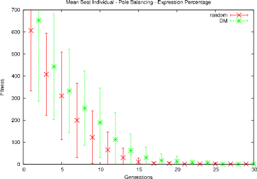
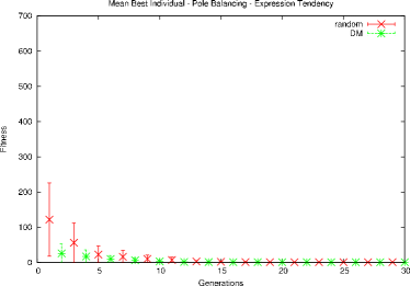
Fig. 2 shows the average fitness evolution for independent runs, for both expression measurement approaches. Both approaches solve the problem quite fast, but it is obvious that using product tendency gives faster convergence to an optimal solution. This is an expected result: when using P-protein absolute values, the concentration of a P-protein has to be fairly close to , in order to provide a solution. However, when using P-protein tendency, the starting concentration of the P-protein has no influence on the behaviour of the cart.
4.1 Generalisation Performance
Whitley et al. [11] proposed a generalisation test to assert whether the discovered solution is robust. Once a controller is evolved that can balance the pole for time steps with a random setup, the evolution cycle is stopped, and this controller is applied to a series of generalisation tests. These consist of combinations of the four input variables, with their normalised values set to the following: , , , , and . This results in initial cases. The generalisation score of the best individual found is thus the number of test cases out of these , for which the controller manages to balance the pole for time steps.
All runs found solutions for this problem, using either P-protein concentrations or P-protein tendencies (for both random and DM-genomes). At the end of each run, the generalisation test was applied to the best individual in the population; Table 1 shows the results obtained.
| Approach | Best | Worst | Median | Mean | Std. Dev. | |
|---|---|---|---|---|---|---|
| Product | random genomes | 422 | 3 | 194 | 202.18 | 110.01 |
| Percentage | DM-genomes | 416 | 23 | 237 | 235.68 | 107.85 |
| Product | random genomes | 359 | 0 | 63 | 85.82 | 66.99 |
| Tendency | DM-genomes | 187 | 7 | 77 | 81.40 | 48.33 |
The results obtained show little difference between random and DM-genomes. However, there is a big difference between using P-proteins concentrations or tendencies, with the former achieving much better results. When using product tendency, the concentration of P-proteins can easily become : the previous move is then repeated, and keeps moving the cart leftwards. This creates a disassociation between the product expression and the cart behaviour, which becomes a handicap when applying the model to some of the harder generalisation tests.
Note that many of the generalisation tests are unsolvable. After an exhaustive search of all possible bang-bang solutions up to steps of simulation, tests were found unsolvable (execution time constrains prevented a deeper search). This means that an ideal controller can only solve (or less) cases. It also shows that the best result found ( tests solved), although not as high as one of the best in the literature ( solved cases [11]), is still quite close to the optimum.
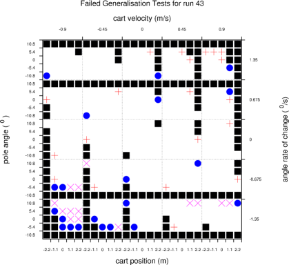
Fig. 3 shows a plot of all the generalisation tests that are not solvable at depth , and those that are additionally not solved by the best random and DM-genome. It shows that cases where and both take large or small values (i.e. a large angle in absolute value, together with a large angular velocity increasing this angle) are unsolvable, and that both genomes additionally fail on cases that are close to these unsolvable cases. It is interesting to see however how the unsolved cases of the DM-genome are mostly symmetric in terms of the matrix of test cases, whereas the random genome is far more unbalanced. This has to do with the sinusoidal nature of the controllers generated by random genomes, as can be seen in the next section.
4.2 Pole balancing behaviour of typical networks
Fig. 4 shows example behaviours of the best evolved regulatory models (random and DM, using P-protein concentrations), applied to different generalisation cases.
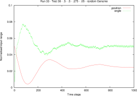
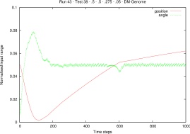
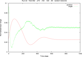
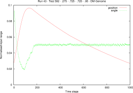
It is interesting to observe the different approaches to solve the same generalisation test. In particular, one can see how the random genome is quite sinusoidal in its approach, whereas the DM-genome generates a much more linear behaviour.
4.3 Resulting Networks: A typical example
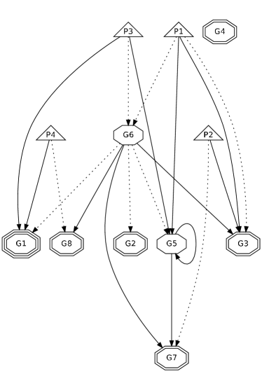
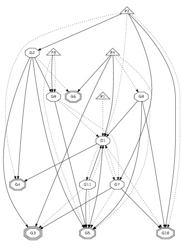
Fig. 5 shows the regulatory networks extracted from the best performing random and DM-genomes, at a threshold of (i.e. only connections with a match larger than 19 are represented, the other ones having a negligible impact on the regulation – see Eq. 1). Even with such a low number of genes, one can see that the regulatory interactions are quite complex. Gene G6 seems to act as a central regulatory node on the random genome, whereas that role is taken up by G1 in the DM-genome. Note also how few connections exist to the chosen P-genes (G1 and G3, respectively); however, the extra protein P4 (representing the rate of change of the pole, ) is directly connected to these on both genomes. This could very well be a mechanism for stronger reaction to changes of , which has been shown to greatly influence the success rate of a balancing attempt (see Fig. 3).
5 Conclusions
One of the main objectives of this paper was to investigate the possibility of using GRNs as a new representation for program synthesis through Genetic Programming. Our motivation was that today’s mainstream Evolutionary Computation (EC) approaches are by and large crude simplifications of the biological paradigm of natural evolution, not taking into account many advances of biological knowledge in the recent past [1]. The artificial GRN model used [6] presents an interesting balance between biological accuracy and computational potential, and was proposed as a good basis to introduce more accurate biological basis for EC.
The results obtained show that there is a clear computational potential within the model; it should therefore be possible to use other similar models as basis for EC techniques.
The adaptation of such models to EC is not straightforward. As these are mostly complex systems, a thorough comprehension of their exact dynamics is often not possible. The choice of how to encode inputs and outputs is also not a simple issue, and can greatly influence their computational potential.
Another key issue is the execution speed. While their biological equivalent systems are extremely fast, at the moment these computer models are somewhat slow, and the model used here is no exception. In order to accelerate the regulatory reactions, several tricks were used, such as adapting the sampling time of the differential equation (the parameter), and parallelization by distributing the evaluation of genomes across a cluster – the resulting average execution time of a single run was around minutes, when executing the code on recent machines running in parallel. Of course, a fascinating possibility to overcome this issue would be to synthesize the resulting GRN into biological medium.
Regarding this problem, some parameters could be optimized (e.g. by evolution). First, the signature and concentration of the extra proteins: a deeper understanding of their influence on the regulatory process is necessary; it could very well be that their influence is far too strong for the moment.
Second, the synchronisation between the biological and physical models. As mentioned before, different models have different reaction times (for example, stabilization times for genomes of this size may go from a few thousand iterations up to hundreds of thousands); each genome would therefore need to tune its synchronisation period individually.
Future work will now focus on extensive testing of the new extended GRN model on various problem domains. The most promising ones seem to be dynamic control problems, as these might profit the most from the remarkable dynamic properties of the model. But the flexibility of this representation allows one to imagine more GP-like approaches. For example, even though only 2 types of proteins were used, a lot more could be introduced - and potentially represent the equivalent of GP functions or terminals. The change of their concentrations over time could then represent priorities of execution, or even probabilities. Work is under way to explore these new avenues of investigation.
References
- [1] W. Banzhaf, G. Beslon, S. Christensen, J. A. Foster, F. Képès, V. Lefort, J. F. Miller, M. Radman, and J. J. Ramsden. From artificial evolution to computational evolution: a research agenda. Nature Reviews Genetics, 7:729–735, 2006.
- [2] M. Kirschner and J. Gerhart. The plausibility of life: Resolving Darwin’s dilemma. Yale University Press, 2005.
- [3] J. Hasty, D. McMillan, F. Isaacs, and J.J. Collins. Computational studies of gene regulatory networks: In numero molecular biology. Nature Reviews Genetics, 2:268–279, 2001.
- [4] M. A. Lones and A. M. Tyrrell. Modelling biological evolvability: Implicit context and variation filtering in enzyme genetic programming. BioSystems, 76((1-3)):229–238, 2004.
- [5] S. Zhan, J. F. Miller, and A. M. Tyrrell. An evolutionary system using development and artificial genetic regulatory networks. In Proc. IEEE CEC’08. IEEE Press, 2008.
- [6] W. Banzhaf. Artificial regulatory networks and genetic programming. In Rick Riolo and Bill Worzel, editors, Genetic Programming Theory and Practice, chapter 4, pages 43–62. Kluwer Publishers, 2003.
- [7] K. Wolfe and D. Shields. Molecular evidence for an ancient duplication of the entire yeast genome. Nature, 387:708–713, 1997.
- [8] M. Kellis, B. W. Birren, and E. S. Lander. Proof and evolutionary analysis of ancient genome duplication in the yeast saccharomyces cerevisiae. Nature, 428:617–624, 2004.
- [9] P. D. Kuo and W. Banzhaf. Small world and scale-free network topologies in an artificial regulatory network model. In J. Pollack, et al., editors, Artificial Life IX, pages 404–409. Bradford Books, 2004.
- [10] A. G. Barto, R. S. Sutton, and C. W. Anderson. Neuronlike adaptive elements that can solve difficult learning control problems. IEEE Transactions on Systems, Man and Cybernetics, 13:834–846, 1983.
- [11] D. Whitley, S. Dominic, R. Das, and C. W. Anderson. Genetic reinforcement learning for neurocontrol problems. Machine Learning, 13(2–3):259–284, 1993.
- [12] I. Rechenberg. Evolutionsstrategie ’94. Frommann-Holzboog, Stuttgart, 1994.