Quantum interference and sub-Poissonian statistics for time-modulated driven dissipative nonlinear oscillator

Abstract

We show that quantum-interference phenomena can be realized for the dissipative nonlinear systems exhibiting hysteresis-cycle behavior and quantum chaos. Such results are obtained for a driven dissipative nonlinear oscillator with time-dependent parameters and take place for the regimes of long time intervals exceeding dissipation time and for macroscopic levels of oscillatory excitation numbers. Two schemas of time modulation: (i) periodic variation of the strength of the ${\chi}(3)$ nonlinearity; (ii) periodic modulation of the amplitude of the driving force, are considered. These effects are obtained within the framework of phase-space quantum distributions. It is demonstrated that the Wigner functions of oscillatory mode in both bistable and chaotic regimes acquire negative values and interference patterns in parts of phase-space due to appropriately time-modulation of the oscillatory nonlinear dynamics. It is also shown that the time-modulation of the oscillatory parameters essentially improves the degree of sub-Poissonian statistics of excitation numbers.

I INTRODUCTION

In recent years the study of quantum dynamics of oscillators with time-dependent parameters has been focus of considerable attention. This interest is justified by many applications in different contexts. Particulary, one application concerns to the center of mass motion of a laser cooled and trapped ion in a Paul trap trapped_ion . The quantum dynamics of an anharmonic oscillator (AHO) with time dependent modulation of its frequency and nonlinearity parameters has been investigated in applications to macroscopic superposition of quantum states time_dep_nonlinearity . In the last few years there has been rapid progress in the construction and manipulation of nanomechanical oscillators with giant ${\chi}(3)$-Kerr nonlinearity nano -nano_2 . The nanomechanical resonator with a significant fourth-order nonlinearity in the elastic potential energy has been experimentally demonstrated A . It has also been shown that this system is dynamically equivalent to the Duffing oscillator with varied driving force duffing_force . This scheme is widely employed for a large variety of applications as well as the other schemes of micro- and nanomechanical oscillators, more commonly as sensors or actuators in integrated electrical, optical, and optoelectrical systems nano , devices .

It is well assessed that in the case of unitary dynamics, without any losses, an anharmonic oscillator leads to sub-Poissonian statistics of oscillatory excitation number, quadratic squeezing and superposition of macroscopically distinguishable coherent states. For dissipative dynamics the important parameter responsible for production of nonclassical states via ${\chi}(3)$ materials is the ratio between nonlinearity and damping. Therefore, the practical realization of such quantum effects requires a high nonlinearity with respect to dissipation. In this direction the largest nonlinear interaction was proposed in many papers, particularly, in terms of electromagnetically induced transparency EM and by using the Purcell effect P , and in cavity QED R . The significant nonlinearity has also been observed for nanomechanical resonators N . These methods can lead to ${\chi}(3)$ nonlinearity of several orders of magnitude higher than natural optical self-Kerr interactions. Note, that high ${\chi}(3)$ nonlinear oscillators generate also a lot of interest recently due to their applications in areas of quantum computing C .

In the case of nonlinear dissipative ${\chi}(3)$ interaction stimulated by coherent driving force, the time evolution cannot be solved analytically for arbitrary evolution times and suitable numerical methods have to be used. Nevertheless, with dissipation included a driven AHO model has been solved exactly in the steady-state regime in terms of the Fokker-Planck equation in complex P representation I . Analogous solution has been obtained for a combined driven parametric oscillator with Kerr nonlinearity II . The Wigner functions for both these models have been obtained using these solutions I , III .

The investigation of quantum dynamics of a driven dissipative nonlinear oscillator for non-stationary cases is much more complicated and only a few papers have been done in this field up to now. More recently, the quantum version of dissipative AHO or the Duffing oscillator with time-modulated driving force has been studied in the series of the papers SR , X1 , X2 in the context of a stochastic resonance SR , quantum-to-classical transition and investigation of quantum dissipative chaos X1 , X2 .

In this paper we continue investigation of time-modulated effects for quantum version of the Duffing oscillator. In this direction we investigate quantum effects in the presence of dissipation and decoherence, mainly sub-Poissonian statistics and signature of quantum interference within the framework of the Wigner function for an oscillatory mode. Two schemas of time modulation: (i) periodic variation of the strength of the ${\chi}(3)$ nonlinearity; (ii) modulation of the amplitude of the driving force will be considered. Our main result is that time modulation of the oscillatory parameters essentially improves the degree of sub-Poissonian statistics of oscillatory excitation numbers as well as leads to negative values of the Wigner functions in an over transient regime for definite time intervals exceeding the transient time within the period of modulation. Thus, we demonstrate that for the case of time-modulated AHO the Wigner function gradually deviates from the Wigner function corresponding to an ordinary AHO without any modulation. Really, surprisingly simple analytical results for the Wigner functions of an ordinary AHO have been analytically obtained in over transient regime I , III , that are positive in all ranges of phase-space. In our scheme the negative values for the Wigner function of oscillatory mode, that reflect quantum-interference patterns in phase space, appear due to time-modulation dynamics and are realized in both bistable and chaotic operational regimes.

Note, that nowadays, large theoretical and experimental papers have been devoted to the implementation of macroscopic (i.e., many particle) quantum superposition states (MQS). The most notable results on MQS are experimentally obtained with atoms interacting with microwave fields trapped inside a cavity SC1 or for freely propagating fields SC2 and with optical parametric amplifier in the presence of decoherence SC3 . Naturally, the question arises whether the quantum-interference patterns obtained for driven AHO can be realized for time intervals exceeding the characteristic decoherence and dissipation time on many particle level. The corresponding results obtained here are verified for the operational regimes of high nonlinearity with respect to dissipation, e.g., for the ratio ${\chi}/{\gamma}\simeq 1\cdot 10^{-1}\div 1.5\cdot 10^{-3}$, where $\chi$ is the nonlinear constant proportional to ${\chi}(3)$ and $\gamma$ is the damping constant. Nevertheless, we have checked for these parameters that phase-space interference patterns are also obtained in the macroscopic level that involves a number of oscillatory excitation numbers in excess of $52$.

The outline of this paper is as follows. In the next section we describe the models and investigate the mean oscillatory excitation numbers and quantum fluctuations of excitation numbers on the base of the Mandel parameters. In Sec. III we shortly discuss the case of the unitary dynamics. In Sec. IV we present the results for the Wigner functions showing negativity due to the time modulations of the oscillatory dynamics. We summarize our results in Sec. V.

II Models: excitation numbers and quantum statistics

We treat the Duffing oscillator as an open quantum system and assume that its time evolution is described by Markovian dynamics in terms of the Lindblad master equation for the reduced density matrix $\rho$. In the interaction picture that corresponds to the transformation $\rho\longrightarrow e^{-i\omega a^{+}at}\rho e^{i\omega a^{+}at}$, where $a^{+}$ and $a$ are the Bose annihilation and creation operators of the oscillatory mode and $\omega$ is the driving frequency, this equation reads in the Markovian form as

$$\frac{d\rho}{dt}=\frac{-i}{\hbar}[H_{0}+H_{int},\rho]+~{}~{}~{}~{}~{}~{}~{}~{}~{}~{}~{}~{}~{}~{}~{}~{}~{}~{}~{}~{}~{}~{}~{}~{}~{}~{}~{}~{}~{}~{}~{}~{}$$

$$\sum_{i=1,2}\left(L_{i}\rho L_{i}^{+}-\frac{1}{2}L_{i}^{+}L_{i}\rho-\frac{1}{2}\rho L_{i}^{+}L_{i}\right).$$ (1)

The Hamiltonians are

$$H_{0}=\hbar\Delta a^{+}a,~{}~{}~{}~{}~{}~{}~{}~{}~{}~{}~{}~{}~{}~{}~{}~{}~{}~{}~{}~{}~{}~{}~{}~{}~{}~{}~{}~{}~{}~{}~{}~{}~{}~{}~{}~{}$$

$$H_{int}=\hbar\chi(t)(a^{+}a)^{2}+\hbar(f(t)a^{+}+f(t)^{*}a),$$ (2)

where $\chi(t)$ and $f(t)$, which may or may not depend on time, represent, respectively, the strength of the nonlinearity and amplitude of the force, $\omega_{0}$ is the resonant frequency, $\Delta=\omega_{0}-\omega$ is the detuning. The dissipative and decoherence effects, losses, and thermal noise are included in the last part of this equation, where $L_{i}$ are the Lindblad operators:

$$L_{1}=\sqrt{(N+1)\gamma}a,\qquad L_{2}=\sqrt{N\gamma}a^{+},$$ (3)

$\gamma$ is the spontaneous decay rate of the dissipation process and $N$ denotes the mean number of quanta of a heat bath.

This model seems experimentally feasible and can be realized in several experimental schemes. In fact, a single mode field is well described in terms of an AHO, and the nonlinear medium could be an optical fiber or a $\chi(3)$ crystal, placed in a cavity. The anharmonicity of mode dynamics comes from the self-phase modulation due to the photon-photon interaction in the $\chi(3)$ medium. In this case, it is possible to realize time modulation of the strength of the nonlinearity by using a media with periodic variation of the $\chi(3)$ susceptibility.

On the other side, the Hamiltonian described by Eq. (2) describes a single nanomechanical resonator with $a^{+}$ and $a$ raising and lowering operators related to the position and momentum operators of a mode quantum motion

$$x=\sqrt{\frac{\hbar}{2m\omega_{0}}}(a+a^{+}),\ p=-i\sqrt{2\hbar m\omega_{0}}(a-a^{+}),$$

where $m$ is the effective mass of the nanomechanical resonator, $\omega_{0}$ is the linear resonator frequency and $\chi$ proportional to the Duffing nonlinearity. One of the variants of nano-oscillators is based on a double-clamped platinum beam N for which the nonlinearity parameter equals to $\chi=\hbar/4\sqrt{3}Qma_{c}^{2}$, where $a_{c}$ is the critical amplitude at which the resonance amplitude has an infinite slope as a function of the driving frequency, $Q$ is the mechanical quality factor of the resonator. In this case, the giant nonlinearity $\chi\cong 3.4\cdot 10^{-4}s^{-1}$ was realized. Note, that details of this resonator, including expression for the parameter $a_{c}$, are presented in amp . On decreasing nanomechanical resonator mass, its resonance frequency increases, exceeding 1 GHz in recent experiments nano , nano_1 . It is possible to reach a quantum regime for such frequencies, i.e., to cool down the temperatures for which thermal energy will be comparable to the energy of oscillatory quanta. The recent investigations in this direction are devoted to classical to quantum transition of a driven nanomechanical oscillator Qnr1 , generation of Fock states Qnr2 , nonlinear dynamics, and stochastic resonance Qnr3 .

Cyclotron oscillations of a single electron in a Penning trap with a magnetic field are another realization of the quantum version of the Duffing oscillator a , b , c . In this case the anharmonicity comes from nonlinear effect that is caused by the relativistic motion of an electron in a trap, while the dissipation effects arise from the spontaneous emission of the synchrotron radiation and thermal fluctuations of the cyclotron motion. Note that a one-electron oscillator allows one to achieve a relatively strong cubic nonlinearity, $\chi/\gamma\lesssim 1$.

For the constant parameters $\chi(t)=\chi$ and $f(t)=f$ the equations (1) and (2) describe the model of a driven dissipative AHO that was introduced long ago in quantum optics to describe bistability due to a Kerr nonlinear medium drumm . For the case of time-dependent parameters $\chi(t)$ and $f(t)$ the dynamics of the AHO exhibits a rich phase-space structure, including regimes of regular, bistable and chaotic motion. We perform our calculations for these three qualitatively different regimes concerning two models of time-modulated AHO corresponding to two physical situations: (i) $\chi=\chi(t)=\chi_{0}+\chi_{1}sin(\delta t)$ and $f(t)=const=f$; (ii) $f=f(t)=f_{0}+f_{1}sin(\Omega t)$ and $\chi(t)=const=\chi$ with $\delta\ll\omega$ and $\Omega\ll\omega$ the modulation frequencies.

We analyze the master equation numerically using quantum state diffusion method (QSD) QSD . According to this method, the reduced density operator is calculated as the ensemble mean

$$\rho(t)=M(|\psi_{\xi}(t)\rangle\langle\psi_{\xi}(t)|)=\lim_{N\rightarrow\infty}\frac{1}{N}\sum_{\xi}^{N}|\psi_{\xi}(t)\rangle\langle\psi_{\xi}(t)|$$ (4)

over the stochastic pure states $|\psi_{\xi}(t)\rangle$ describing evolution along a quantum trajectory. The stochastic equation for the state $|\psi_{\xi}(t)\rangle$ involves both Hamiltonian described by Eq. (2) and the Linblad operators described by Eq. (3). We calculate the density operator using an expansion of the state vector $|\psi_{\xi}\rangle$ in a truncated basis of Fock’s number states of a harmonic oscillator

$$|\psi_{\xi}(t)\rangle=\sum_{n}a_{n}^{\xi}(t)|n\rangle.$$ (5)

II.1 Improvement of the sub-Poissonian statistics by modulation of the nonlinearity

In the classical limit the corresponding equation of motion for the dimensionless mean amplitude $\alpha=Tr(\rho a(t))$ has the form

$$\frac{d\alpha}{dt}=-\frac{\gamma}{2}\alpha-i(\Delta+(\chi_{0}+\chi_{1}\sin\delta t)(1+2|\alpha|^{2}))\alpha-if.$$ (6)

We remind the reader that for the constant strength of the nonlinearity, $\chi_{1}=0$, the semiclassical mean excitation number $|\alpha|^{2}$ as a function of the driving intensity can exhibit multiple steady states and hysteresis. In the case of modulation, $\chi_{1}\neq 0$, the interaction Hamiltonian is explicitly time dependent, and the system exhibits regions of regular, bistable, and chaotic motion with $\chi_{0}$, $\chi_{1}$, $\Delta$, and the modulation frequency being the control parameters.

We examine these operational regimes by numerical analysis of the phase space of dimensionless position and momentum $x=Re(\alpha)$ and $y=Im(\alpha)$. Choosing $x_{0}$ and $y_{0}$ as an arbitrary initial phase-space point of the system at the time $t_{0}$, we define a constant phase map in the $(X,Y)$ plane by the sequence of points $(X_{n},Y_{n})=(X(t_{n}),Y(t_{n}))$ at $t_{n}=t_{0}+\frac{2\pi}{\delta}n$ ($n=0,1,2,...$). This means that for any $t=t_{n}$ the system is at one of the points of the Poincaré section. The analyses show that for time scales exceeding the damping time $1/\gamma$, the asymptotic dynamics of the system is regular in the limits of small and large values of the modulation frequency, i.e., $\delta\ll\gamma$, $\delta\gg\gamma$, and for positive values of the detuning, $\Delta>0$. Such regime is also realized when the modulation part of the parameter, i.e., $\chi_{1}$ is much less than the $\chi_{0}$.

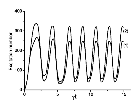
Figure 1: The photon excitation numbers for two cases: (1) for monostable regime with parameters $\Delta/\gamma=0.1,\chi(t)/\gamma=5\cdot 10^{-3}(1+0.7\sin(\delta t)),\delta/\gamma=3,f/\gamma=20$; (2) for bistable regime with parameters $\Delta/\gamma=-1,\chi(t)/\gamma=6\cdot 10^{-3}(1+0.5\sin(\delta t)),\delta/\gamma=3,f/\gamma=20$.

First, we discuss the case of classically regular behavior assuming the interaction of the system with vacuum reservoir: $N=0$. Below we present numerical results for both the oscillatory mean excitation number $\langle n\rangle=M(\langle\psi_{\xi}|a^{+}a|\psi_{\xi}\rangle)$ and Mandel $Q$ parameter which describes the deviation of excitation number uncertainty from the Poissonian variance, i.e., $Q=\frac{\langle(\Delta n)^{2}\rangle-\langle n\rangle}{\langle n\rangle}$, $\langle(\Delta n)^{2}\rangle=\langle(a^{+}a)^{2}\rangle-\langle a^{+}a\rangle^{2}$, i.e.,

$$\langle(\Delta n)^{2}\rangle=M(\langle\psi_{\xi}|(a^{+}a)^{2}|\psi_{\xi}\rangle)-\langle n\rangle^{2}.$$ (7)

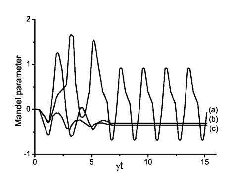
Figure 2: The Mandel parameter for the monostable regime with the parameters as in Fig. 1, case (1), (curve(a)); AHO without time-modulation: $\chi/\gamma=8.5\cdot 10^{-3}$ (b); $\chi/\gamma=1.5\cdot 10^{-3}$ (c). The other parameters are as in the Fig. 1, case (1).

For the driven dissipative AHO under time-modulation of the strength of nonlinearity, the ensemble-averaged mean oscillatory excitation number exhibits a periodic time-dependent behavior in both cases of regular and chaotic regimes for over transient time-intervals. For bistable and monostable regimes the results of numerical calculations for time evolution of $\langle n\rangle$ are depicted in Fig. 1(case 1) and Fig. 1(case 2) for the parameters: $\chi(t)/\gamma=5\cdot 10^{-3}(1+0.7\sin(3\gamma t))$ and $\chi(t)/\gamma=6\cdot 10^{-3}(1+0.5\sin(3\gamma t))$. The time evolution of the Mandel parameter is depicted on Fig. 2. As we see (Fig. 2(a)), the $Q$ parameter also shows a time-dependent modulation and formation of the sub-Poissonian statistics $(Q<0)$ for the definite time intervals exceeding the transient time $t\gamma\geq 6$. The level of the oscillatory excitation-number fluctuations reaches to the minimum values $Q_{min}=-0.69$ and the maximum values $Q_{max}=1.2$ at the fixed intervals of time, respectively, at $\gamma t_{k}=6.8+\frac{2\pi k}{\delta}\gamma$ and at $\gamma t_{k}=7.6+\frac{2\pi k}{\delta}\gamma$ , $(k=0,1,2...)$. Comparing this result with the case without any time-modulation we also present the $Q$ parameter for the maximal and minimal values of $\chi(t)$, i.e., for $\chi=8.5\cdot 10^{-3}$ ($Q=-0.3$, curve (b)) and for $\chi=1.5\cdot 10^{-3}$ ($Q=-0.36$, curve (c)). Thus, we conclude that the modulation of the strength of nonlinearity leads to the improvement of the level of sub-Poissonian statistics below the level of corresponding steady-state regime. Indeed, we find that $Q_{min}<-0.36$. It is interesting that $Q_{min}$ corresponds to the maximal value of the mean excitation number, $\langle n\rangle=249$. As calculations show, analogous result takes place for the bistable regime, Fig. 1, case(2). In this case, $Q_{min}=-0.7$ for the mean excitation numbers $\langle n\rangle=352$. Note that such effect of improving the sub-Poissonian statistics has been recently obtained for the dissipative AHO under time-modulation of the driving amplitude X1 .

III Time modulation in the case of unitary dynamic

We now calculate the quantum distributions, at first considering the simplest case of non-dissipative AHO without any driving. In this case the operator $(a^{+}a)$ is an invariant of motion, since this operator commutes with the corresponding Hamiltonian $H(t)=\hbar[\Delta a^{+}a+\chi(t)(a^{+}a)^{2}]$. The system exhibits an unitary evolution; for an initial coherent state $|\alpha_{0}\rangle$ with the phase $\varphi=0$ at $t=0$, the state evolution at time $t$ is

$$|\psi(t)\rangle=U\left(t\right)|\alpha_{0}\rangle=e^{-|\alpha_{0}|/2}\sum_{n=0}^{\infty}\frac{|\alpha_{0}|^{n}}{\sqrt{n!}}e^{-i\varphi(t)n^{2}}|n\rangle,$$ (8)

, where $\varphi(t)=\int_{0}^{t}\chi(\tau)d\tau$. This state involves the time-modulation effects as well as describes the interference of the Fock number states $|n\rangle$. The corresponding nonstationary Wigner function is written as

$$W(\alpha,t)=\frac{2}{\pi^{2}}e^{-2|\alpha|^{2}}\int d^{2}\beta\langle-\beta|\psi(t)\rangle\langle\psi(t)|\beta\rangle e^{-2(\beta\alpha^{*}-\beta^{*}\alpha)}.$$ (9)

We transform this formula to the form

$$W(r,\theta)=\sum_{n,m}\rho_{nm}(t)W_{mn}(r,\theta),$$ (10)

where $(r,\theta)$ are the polar coordinates in the complex phase-space plane, $x=rcos\theta$, $y=rsin\theta$, while the coefficients $W_{mn}(r,\theta)$ are the Fourier transform of matrix elements of the Wigner characteristic function

$$W_{mn}\left(r,\theta\right)=\left\{\begin{array}[]{rcl}\frac{2}{\pi}\left(-1\right)^{n}\sqrt{\frac{n!}{m!}}e^{i(m-n)\theta}(2r)^{m-n}e^{-2r^{2}}L_{n}^{m-n}(4r^{2}),~{}m\geq n\\ \frac{2}{\pi}\left(-1\right)^{m}\sqrt{\frac{m!}{n!}}e^{i(m-n)\theta}(2r)^{n-m}e^{-2r^{2}}L_{m}^{n-m}(4r^{2}),~{}n\geq m\end{array},\right.$$ (13)

The matrix elements $\rho_{nm}(t)=\langle n|\psi(t)\rangle\langle\psi(t)|n\rangle$ are equal to

$$\rho_{nm}(t)=e^{-|\alpha_{0}|^{2}}\frac{|\alpha_{0}|^{n+m}}{\sqrt{n!m!}}e^{i\varphi(t)(n^{2}-m^{2})},$$ (14)

where for $\chi(t)=\chi_{0}+\chi_{1}sin(\delta t+\phi)$ we have

$$\varphi(t)=\chi_{0}t+\frac{\chi_{1}}{\delta}[\cos(\delta t+\phi)-\cos\phi].$$ (15)

These results are valid for short time intervals, much less than the characteristic dissipation time, $t\ll\gamma^{-1}$. The Wigner function Eq. (10) with the density matrix Eq. (14) leads to the interference fringes arising from the non-diagonal elements $\rho_{nm}$. For non-modulated case, $\varphi(t)=\chi_{0}t$, the Wigner function is well studied (see, for example, cccc ). Particularly, for $\chi t=\frac{\pi}{2}$ and in the case of the initial coherent state, it describes a superposition of other coherent states of the same amplitude but different phases. The novelty of the Eqs. (10) and (14) consists in the time-dependent nonlinearity that is the factor of $\varphi(t)$. This modulation term allows to control the time intervals of the maximal superposition with appropriate choice of the modulation frequency and the phase $\phi$. Indeed, the first time at which we have the superposition of coherent states is determined from $\varphi(t)=\frac{\pi}{2}$. Particularly, for $\delta t\ll 1$, we have $\varphi(t)\simeq(\chi_{0}+\chi_{1}\sin\phi)t$ and hence the superposition is realized, if $t=\pi/2(\chi_{0}+\chi_{1}\sin\phi)$.

IV Wigner functions and quantum-interference patterns

It is well known that the phase-space Wigner distribution function can simply visualize nonclassical effects including quantum-interference. For example, a signature of quantum interference is exhibited in the Wigner function by the non-positive values. In this section the numerical results of the nonstationary Wigner functions in bistable and chaotic regimes of AHO are presented and discussed.

It should be noted that the most of investigations of the quantum distributions of oscillatory states, including also modes of radiations, have been made for the steady-state situations. The simplicity of Kerr nonlinearity allows to determine the Wigner function of the quantum state under time evolution due to interaction (see, for example cccc ). In this sense, we note the main peculiarity of our paper in comparison with above noted important inputs. In this paper, we calculate the Wigner functions in an over transient regime, $t\gg\gamma^{-1}$, of the dissipative dynamics, however, we consider time-dependent effects which appear due to the time-modulation of the oscillatory parameters.

Below we investigate the Wigner functions for both cases of time-modulation (see, cases (i) and (ii)). For periodic variation of the strength of $\chi(3)$ nonlinearity, semiclassical dynamics is described by Eq. (6), while for the case of time-modulation of the driving amplitude the semiclassical equation reads as

$$\frac{d\alpha}{dt}=-\frac{\gamma}{2}\alpha-i(\Delta+\chi_{0}(1+2|\alpha|^{2}))\alpha-i(f_{0}+f_{1}sin(\Omega t)).$$ (16)

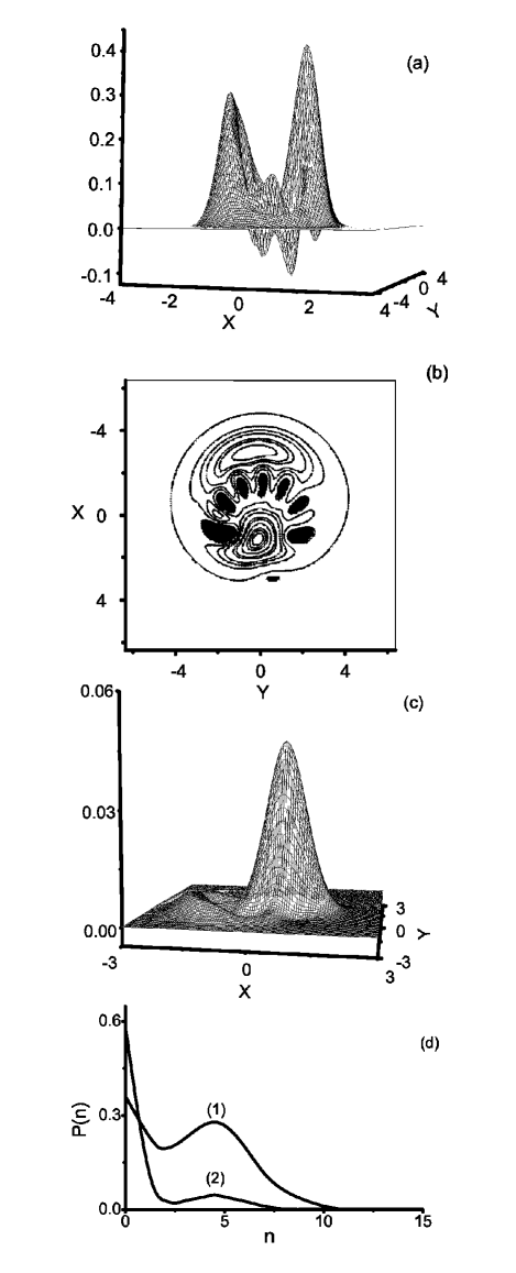
Figure 3: The Wigner function and its contour plot, averaged over 3000 trajectories, for the parameters: $\Delta/\gamma=-15,\chi/\gamma=2,f/\gamma=5.8(1+0.5\sin(\Omega t)),\Omega/\gamma=2$, (a) and (b). The contour plot of the Wigner function that indicates the ranges of negativity in the black (b). The Wigner function for AHO without modulation, $f/\gamma=5.8$ (c). The probability distribution of excitation numbers (d): case of time-modulation (1), case without of modulation (2). The parameters are as on the Figs. (a) and (c), respectively.

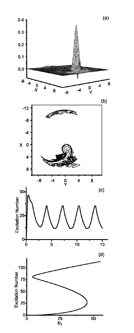
Figure 4: The Wigner function (a); the contour plot of the Wigner function (b); and the mean excitation number (c); averaged over 3000 trajectories, for the dissipative AHO under time-modulated driving. The parameters are in the range of bistability: $\Delta/\gamma=-13.02,\chi/\gamma=0.08,f/\gamma=29(1+0.5\sin(\Omega t)),\Omega/\gamma=2$. The hysteresis curve (d) for the stationary case.

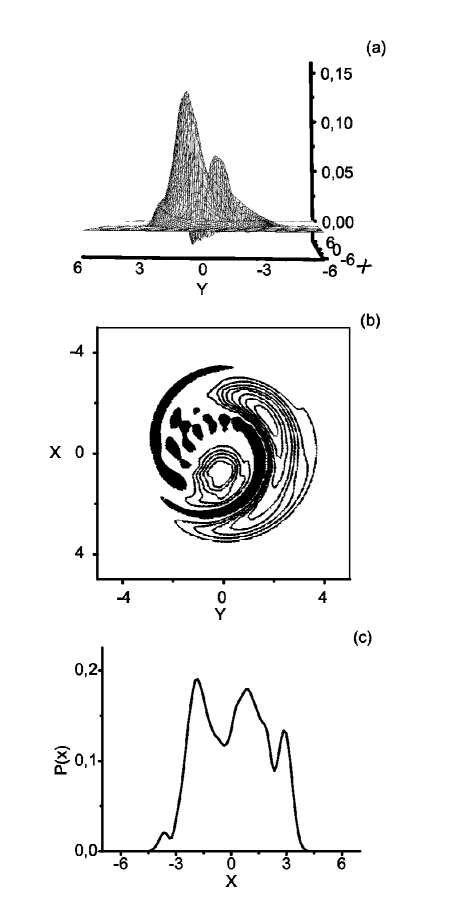
Figure 5: The Wigner function (a); the contour plot of the Wigner function (b); and the distribution of quadrature amplitude $P(x)$ for the driven dissipative AHO with time-modulation of the nonlinearity. The parameters are in the range of bistability: $\Delta/\gamma=-15,\chi(t)/\gamma=1.5(1+0.5\sin(\delta t)),\delta/\gamma=5,f/\gamma=10.2$.

IV.1 Quantum interference pattern assisted by the bistability.

First, we consider the case of time-modulated driving force. In the limit $f_{1}\ll f_{0}$ the system is reduced effectively to the model of a single driven anharmonic oscillator, which exhibits bistability for the definite range of the parameters: $\chi_{0}$, $\Delta$, $f_{0}$, and $\gamma$ (see for example duffing_force , SR , c , drumm ), however, for negative detuning, $\Delta<0$. In this case, the semiclassical steady-state oscillatory excitation number $|\alpha|^{2}$, as solution of Eq. (16), displays hysteresis behavior, while quantum mechanical mean excitation number $\langle a^{+}a\rangle$ does not show any hysteresis in the critical range due to quantum statistical averaging I . The analysis of the stochastic trajectories for an expectation number $n_{\xi}(t)=\langle\psi_{\xi}|a^{+}a|\psi_{\xi}\rangle$ shows that the system spends most of its time close to one of the semiclassical bistable solutions with quantum-interstate transitions, occurring at random intervals SR . On increasing the amplitude $f_{1}$ a new channel of stimulated interstate transitions is raised between the semiclassical bistable solutions. Their contribution for the further increasing of $f_{1}$ at $f_{1}\leq f_{0}$ leads to the emergence of a chaotic regime.

In another scenario of transition from regular regime to bistability and chaos the modulation frequency $\Omega$ may be varied, with the other parameters unchanged. In the range $\Omega\ll\gamma$ the modulation of the system is adiabatic. On increasing modulation frequency the system oscillates between the two possible metastable states. At $\Omega\geq\gamma$ a strong entanglement of these states occurs, and the system comes to a chaotic regime. As can be seen from the numerical calculations, the analogous results are also obtained from the case (i), i.e., for the case of modulation of the parameter $\chi(t)$. Some differences between operational regimes of these two models will be considered below.

The Wigner function is determined by the expression

$$W(\alpha,t)=\frac{2}{\pi^{2}}e^{-2|\alpha|^{2}}\int d^{2}\beta\langle-\beta|\rho(t)|\beta\rangle e^{-2(\beta\alpha^{*}-\beta^{*}\alpha)},$$ (17)

which is obtained from the Eq. (10), where, however, the matrix elements of the density operator of the full dissipative system are used, $\rho_{nm}(t)=M(\langle n|\psi_{\xi}(t)\rangle\langle\psi_{\xi}(t)|m\rangle)$. The coefficients $W_{mn}(r,\theta)$ are the Fourier transform of matrix elements of the Wigner characteristic function (see Eq. (13)).

As calculations show, the most striking signature of quantum bistability in the presence of time-modulation is the appearance of quantum-interference with negative regions in the Wigner function. We illustrate quantum-interference pattern in phase space and in the bistable operational regime on Figs. 3-4. More importantly, we clearly observe (Fig. 3(a)) that the Wigner function displays two peaks around the bistable semiclassical solutions as well as the negative part between them that indicates quantum-interference. The ranges of negativity are indicated in details on Fig. 3(b). Another peculiarity is that the Wigner function is nonstationary and the interference patterns take place for the definite time intervals $\gamma t_{k}=6.9+\frac{2\pi k}{\delta}\gamma$ (k=0,1,2…), exceeding transient time, at which the mean excitation number $\langle n\rangle$ reaches its maximal value. The interference pattern is destroyed as the time-modulation is decreased. Indeed, as it is shown on Fig. 3(c), in the case $f_{1}=0$ the Wigner function is positive in all phase-space and indicates quantum bistability in accordance with the analytical results I . Examples of the curves for the ensemble-averaged excitation number distributions $P_{n}=\langle n|\rho|n\rangle$ are demonstrated on Fig. 3(d) for the two cases of modulated and non-modulated dynamics described on the Figs. 3(a) and 3(c). In correspondence with the bistable behavior of the system we find a developing bimodal structure of $P_{n}=\langle n|\rho|n\rangle$ for the oscillatory mode. However, this structure is less pronounced for the case of non-modulated stationary dynamics and is well resolved for the case of time-modulation of the driving force, as we can also observe from the results for the Wigner functions. The reason is that the interstate transitions due to time-modulation of the driving force approximately equalizes the populations of the states.

Note, that these results are given for a choice of parameters which ensures that the oscillator is in the specific bistable regime operating with small main excitation numbers. Nevertheless, it is possible to find the parameters that would enable us to observe quantum-interference pattern on a macroscopic level of excitation numbers. For this goal, we use the scaling properties of the driven AHO recently proposed in X1 . Indeed, it is easy to verify that Eqs. (6) and (16) are invariant with respect to the following scaling transformation of the amplitude $\alpha\rightarrow\alpha^{{}^{\prime}}=\lambda\alpha$, where $\lambda$ is a real positive dimensionless coefficient, if the oscillatory parameters are correspondingly transformed as $\Delta\rightarrow\Delta^{{}^{\prime}}=\Delta+\chi(1-1/\lambda^{2})$, $\chi\rightarrow\chi^{{}^{\prime}}=\chi/\lambda^{2}$, $f\rightarrow f^{{}^{\prime}}=\lambda f$, $\gamma\rightarrow\gamma^{{}^{\prime}}=\gamma$. This scaling properties of the semiclassical equations signifies that for the definite different sets of the parameters the phase-space trajectories have the same form and differ from each other only in a scale. It has been numerically shown that this scaling parameter is also approximately realized in a quantum ensemble theory in the presence of quantum noise, for wider ranges of the parameters, but not for large values of the parameter $\chi/\gamma$, i.e., in a deeper quantum regime. We calculate the Wigner function and its contour plot for the parameters obtained from the data of the Fig. 3(a) with the scaling parameter $\lambda=5$. The results presented in Fig. 4(a) and Fig. 4(b), particularly, illustrate the quantum interference pattern for a macroscopic level of the mean excitation number, $\langle n\rangle=40$. As we see, the negative part of the Wigner function decreases with increasing the mean oscillatory excitation number. The result for time evolution of the mean oscillatory excitation number averaged over quantum trajectories is depicted in Fig. 4(c). For such parameters the system still operates in a bistable regime. We indicate the hysteresis curve for the corresponding semiclassical solution for the excitation number $|\alpha|^{2}$ on Fig. 4(d) for the stationary case: $f_{1}=0$.

Analogous results are obtained for the case (i), that is the time-modulation of the strength of the nonlinearity. The results of numerical calculations of the Wigner function and the corresponding distribution of quadrature amplitude P(x) in the operational regime of bistability are shown on Fig. 4.

Note that these interference effects have been demonstrated for the strong quantum regimes of high nonlinearity. As a consequence, the oscillatory excitation number is small in this bistable regime. Below we consider the regime of chaotic dynamics where quantum-interference pattern is realized with relatively high level of excitation numbers.

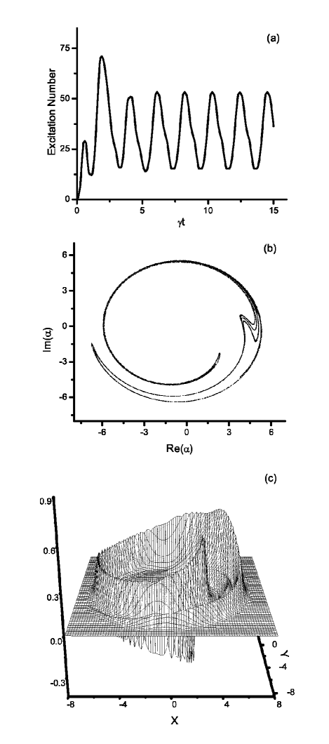
Figure 6: (a) The mean excitation number; (b) the Poincar$\acute{e}$ section ($\approx 20000$ points) for the dimensionless complex amplitude $\alpha$, plotted at times of the constant phase $\delta t_{k}=2\pi k$ (k=0,1,2…), when the maximal interference pattern on the Wigner function (c) is realized, for the case of time-modulated nonlinearity $\chi(t)$. The parameters are in the range of chaos: $\Delta/\gamma=-5,\chi(t)/\gamma=0.2(1+0.75\sin(\delta t)),\delta/\gamma=3,f/\gamma=10$.

IV.2 Negative Wigner functions for the chaotic dynamics.

For both models of AHO corresponding to two forms of time-modulations (cases (i) and (ii)), the dynamics of the system is chaotic in the ranges: $\delta\geq\gamma$ or $\Omega\geq\gamma$ and $\chi_{0}\simeq\chi_{1}$ or $f_{0}\simeq f_{1}$ and for negative detuning. Thus, the ways to realize the controlling transition from the regular to chaotic dynamics through the intermediate ranges of bistability are to vary the strength $\chi_{1}$ or $f_{1}$ of the modulation processes in the ranges from $\chi_{1}\ll\chi_{0}$ or $f_{1}\ll f_{0}$ to $\chi_{1}\leq\chi_{0}$ or $f_{1}\leq f_{0}$. In order to get a quantitative measure for chaotic dynamics, we have chosen the analysis on the base of the $Poincar\acute{e}$ section.

We note, that the order-to-chaos transition for dissipative AHO under time-modulated driving force was already analyzed X1 . Therefore, here we concentrate on investigation of quantum interference phenomenon considering AHO with time-modulated nonlinearity. The results of the ensemble-averaged numerical calculation of the mean excitation number, the Poincar$\acute{e}$ section and the Wigner function are shown on Figs. 6(a)-6(c), respectively. The mean excitation number of the driven AHO versus dimensionless time is depicted in Fig. 6(a). In contrast to the semiclassical result its quantum ensemble counterpart (Fig. 6(a)) has clear regular periodic behavior for time intervals exceeding the characteristic dissipation time, due to ensemble averaging. The Fig. 6(b) clearly indicates the classical strong attractors with fractal structure that are typical for a chaotic $Poincar\acute{e}$ section. Thus, the Wigner function Fig. 6(c) reflects the chaotic dynamics, its contour plots in the (x,y) plane are similar to the $Poincar\acute{e}$ section. However, the Wigner functions have regions of negative values for the definite time intervals. The example depicted on Fig. 6(c) corresponds to time intervals $\gamma t_{k}=6+\frac{2\pi k}{\delta}\gamma$ (k=0,1,2…), for which the mean excitation number reaches a macroscopic level, i.e., $n=52$.

V CONCLUSION

We have numerically studied the phenomena at the overlap of bistability, chaos and quantum-interference for the driven and damped AHO with time-dependent parameters. We have pointed out, that the time-modulation of the oscillatory parameters, that are the strength of $\chi(3)$ nonlinearity or the amplitude of the driving force, leads to formation of the quantum-interference patterns in phase-space in over transient regimes, for the definite time intervals exceeding the transient dissipation time $t\gg\gamma^{-1}$. These effects are displayed as the negative values of the Wigner functions in phase-space. Quantum interference patterns take place for both bistable and chaotic operational regimes and come from the oscillation between possible metastable states of semiclassical dynamics due to time-modulation. We have also demonstrated that the time-modulation of the nonlinearity parameter for the regular operational regime of AHO, essentially improves the degree of sub-Poissonian statistics of oscillatory mean excitation number. In this spirit, we emphasize that the idea of improving the degree of quantum effects as well as obtaining qualitatively new quantum effects due to appropriately time-modulation of open quantum systems was recently exploited for formation of high degree continuous variable entanglement in nondegenerate optical parametric oscillator ENT .

- (1) F. Diedrich, J. C. Berquist, W. M. Itano, and D. J. Wineland, Phys. Lett. 62, 403 (1989); D. J. Wineland, C. Monroe, W. M. Itano, D. Liebfred, B. E. King and D. M. Mekhot, J. Res. Natn. Inst. Standt. Technol. 103, 259 (1998).
- (2) S. Mancini and P. Tombesi, Phys. Rev. A52, 2475 (1995).
- (3) X. M. H. Huang, C. A. Zorman, M. Mehregany, and M. L. Roukes, Nature (London) 412, 496 (2003); K. C. Schwab and M. L. Roukes, Phys. Today 58, N7, 36 (2005).
- (4) A. N. Cleland and M. R. Geller, J. App. Phys. 92, 2758 (2002); A. N. Cleland and M. R. Geller, Phys. Rev. Lett. 93, 070501 (2004).
- (5) K. Jacobs and A. J. Landahl, arXiv: 0809.2993v1 quant-ph (2008).
- (6) R. Almog, S. Zaitsev, O. Shtempluck, and E. Buks, Phys. Rev. Lett. 98, 078103 (2007).
- (7) E. Babourine-Brooks, A. Doherty, G. J. Milburn, quant-ph/ 0804.3618v1, (2008).
- (8) M. P. Blencowe, Phys. Rep. 395 159 (2004); T. J. Kippling and K. J. Vahala, Opt. Expr. 15,17172 (2007); M. Aspelmeyer and K. Schwab, New J. Phys. 10, 095001 (2008).
- (9) A. Imamoglu, H. Schmidt, G. Woods, and M. Deutsch, Phys. Rev. Lett. 79, 1467 (1997); M. J. Werner and A. Imamoglu, Phys. Rev. A 61 011801(R) (1999); M. Fleischhauer A. Imamoglu, and J. P. Marangos, Phys. Mod. Phys. 77, 633 (2005).
- (10) P. Bermel, A. Rodriguez, J. D. Joannopoulos, and M. Soljacic, Phys. Rev. Lett. 99, 053601 (2007).
- (11) F. G. S. L. Brandao, M. Hertmann, and M. B. Plenio, New J. Phys. 10, 043010 (2008).
- (12) I. Kozinsky, H. W. Ch. Postma, O. Kogan, A. Husain and M. L. Roukes, Phys. Rev. Lett. 99, 207201 (2007).
- (13) Q. A. Turchette , C. J. Hood, W. Lange, H. Mabuchi, and H. J. Kimble, Phys. Rev. Lett. 75, 4710 (1995); K. Nemoto, W. J. Munro, Phys. Rev. Lett. 93, 250502 (2004); W. J. Munro, K. Nemoto and T. P. Spiller, New J. Phys. 7, 137 (2005); J. Lee, M. Paternostro, C. Ogden, Y. W. Cheong, S. Bose and M. S. Kim, New J. Phys. 8, 23 (2006).
- (14) K. V. Kheruntsyan J. Opt. B: Quantum Semiclass. Opt. 1, 225 (1999).
- (15) G. Yu. Kryuchkyan and K. V. Kheruntsyan Opt. Commun 120, 132 (1996).
- (16) K. V. Kheruntsyan D. S. Krahmer, G. Yu. Kryuchkyan and K. G. Petrossian, Opt. Commun 139, 157 (1997).
- (17) H. H. Adamyan, S. B. Manvelyan, and G. Yu. Kryuchkyan Phys. Rev. A63, 022102 (2001).
- (18) G. Yu. Kryuchkyan and S. B. Manvelyan, Phys. Rev. Lett. 88, 094101 (2002); Phys. Rev. A68, 013823 (2003).
- (19) H. H. Adamyan, S. B. Manvelyan, and G. Yu. Kryuchkyan Phys. Rev. E64, 046219 (2001).
- (20) M. Brune, et al, Phys. Rev. A45,5193 (1992); J. M. Raimoind, et al, Rev. Mod. Phys. 73, 565(2001).
- (21) A. Ourjoumtsev, et al, Science. 382,83 (2006); A. Ourjoumtsev, et al, Nature 448, 787 (2007).
- (22) F. DeMartini, et al, Phys. Rev. Lett. 100, 253601 (2008).
- (23) H. W. Ch. Postma, I. Kozinsky, A. Hussian, and M. L. Roukes, Appl. Phys. Lett. 86, 223105 (2005).
- (24) I. Katz, A. Retzker, R. Straub, and R. Lifshitz, Phys. Rev. Lett. 99 040404 (2007).
- (25) E. Buks, E. Segev, S. Zaitsev, B. Abdon, and M. P. Blencowe, Europhys. Lett., 81 10001 (2008).
- (26) R. Almog, S. Zaitsev, O. Shtempluck, and E. Buks, App. Phys. Lett. 90, 013508 (2007); J. S. Aldridge and A. H. Cleland, Phys. Rev. Lett 94, 156403 (2005).
- (27) A. E. Kaplan, Phys. Rev. Lett. 48, 138 (1982).
- (28) D. Enzer and G. Gabrielse, Phys. Rev. Lett. 78, 1211 (1997); G. Gabrielse, H. G. Dehmelt, and W. Kells, ibid. 54, 537 (1985).
- (29) M. Rigo, G. Alber, F. Mota-Furtado, and P. F. OMahony, Phys. Rev. A55, 1665 (1997); A58, 478 (1998).
- (30) P. D. Drummond and D. F. Walls, Phys. Rev. A 23 2563 (1981).
- (31) N. Gisin and I. C. Percival, J. Phys. A 25, 5677 (1992); 26, 2233 (1993); 26, 2245 (1993); I. C. Percival, Quantum State Diffusion(Cambridge University Press, Cambridge, (2000).
- (32) , G.J. Milburn and K. Wodkiewicz, arXiv:quant-ph/060516v4.
- (33) H. H. Adamyan and G. Yu. Kryuchkyan, Phys. Rev. A74, 023810 (2006); N. H. Adamyan, H. H. Adamyan and G. Yu. Kryuchkyan, Phys. Rev. A77, 023820 (2008).