A two dimensional adaptive nodes technique in irregular regions applied to meshless-type methods

Abstract

We propose a two dimensional (2D) adaptive nodes technique for irregular regions. The method is based on equi-distribution principal and dimension reduction. The mesh generation is carried out by first producing some adaptive nodes in a rectangle based on equi-distribution along the coordinate axes and then transforming the generated nodes to the physical domain. Since the produced mesh is applied to the meshless-type methods, the connectivity of the points is not used and only the grid points are important, though the grid lines are utilized in the adapting process. The performance of the adaptive points is examined by considering a collocation meshless method which is based on interpolation in terms of a set of radial basis functions. A generalized thin plate spline with sufficient smoothness is used as a basis function and the arc-length is employed as a monitor in the equi-distribution process. Some experimental results will be presented to illustrate the effectiveness of the proposed method.
Key words. Adaptive mesh, Equi-distribution, Irregular regions, Collocation meshless method, Dimension reduction method.

1 Introduction

Mesh free methods are now well known in the numerical solution of partial differential equations (PDEs). The most attractive feature of these techniques is that discretization of the domain or boundary is not required. This feature considerably reduces the computational complexity of the method. While the meshless techniques are often divided into two categories: boundary (see for example [20]) and domain type methods, the current work concerns with the latter category.
The use of radial basis functions (RBFs) for solving PDEs, first presented by Kansa, is a fully mesh free approach and falls into the domain type matheds [12, 24]. This method can be easily applied to the case of higher dimensional spaces due to the nature of the RBFs. Despite a good performance of RBFs in approximating multi-variate functions, they involve ill-conditioning, especially for large scale problems. Another difficulty concerns their computational efficiency, due to the dense matrices arising from interpolation. To tackle the above difficulties some sort of localization, such as domain decomposition methods (DDM) [8] and compactly supported RBFs (CS-RBFs) [5], the most important of which was introduced by Wendland [21], have been recommended.
In the DDM the domain is divided into some subdomains and the PDE is solved for each subproblem followed by assembling the global solution. As a result, the ill-conditioning is avoided and the computational efficiency is improved due to working with small size matrices. On the other hand, using the CS-RBFs results in sparse matrices, which again improve the conditioning and computational efficiency of the method.

This work involves a different approach which can still be used with the above proposed methods. As was highlighted before, in using the classical RBFs, increasing the size of the problem itself affects the conditioning. Consequently, reducing the number of nodes can improve the conditioning. One way to achieve this goal is to apply a set of adaptive nodes rather than uniform ones. As is well known, the main idea in adaptive meshes is to use a minimum number of nodes while still having the desired accuracy. This is achieved by allocating more mesh points to the areas where they are required. The adaptive mesh strategies often fall into two categories: the equi-distribution principle [7] and the variational principle [23]. The most popular technique, which has been widely used in the literature, is based on the equi-distribution strategy, which is also employed in this work. In this approach the mesh distribution is carried out in such a way that some measure of error, called a monitor function, is equalized over each subinterval.

Much effort has been devoted to generating adaptive meshes in two and three dimensional spaces, based on both equi-distribution and variational principles (see for example [18, 2, 15]). In the literature two major methods, namely transformation [6] and dimension reduction [19], have been employed to produce 2D meshes. The first category is based on mapping the physical domain into a simple domain with a uniform mesh and it leads to solving a differential equation in order to obtain an adaptive mesh. In the dimension reduction method, which is also employed in this paper, the equi-distribution process is reduced to a 1D case.

A method based on equi-distributing along the grid lines in the coordinate directions has been presented to produce mesh points in rectangular regions [16]. Also a generalization of this method to the case of three dimensions was proposed in [17]. However, due to the use of grid lines in the coordinate directions, this method was limited to the case of rectangular and cubic domains, respectively, in the case of 2D and 3D. The purpose of the current work is to extend the above method to more general cases with irregular boundaries in 2D. This is carried out by first, generating some adaptive nodes in a rectangle, then mapping the generated nodes to the physical domain employing a suitable transformation. Of course, the mesh produced by the proposed method neither precisely satisfies the equi-distributing condition nor concerns about properties such as orthogonality, which are often required in numerical mesh-dependent methods. Instead, the mesh points are suitable for any meshless methods in which the mesh points, rather than mesh lines, are important.

While a part of researches in the adaptive mesh community concerns with constructing monitor functions for different applications [3], the current study focus on the mesh generation strategy using a well known monitor, namely arc-length [22]. In addition, we remark that the connectivity of the mesh are not used in this work, although they are used in the mesh points generation process.
This paper is organized as follows. In section 2 the adaptive mesh technique in 1D is reviewed. A generalization of this method to the case of 2D is discussed in section 3. The new mesh generation method is presented in section 4. In section 5 the collocation meshless method is reviewed. Some numerical results are given in section 6.

2 Adaptive mesh

We now introduce the concept of equi-distribution in the case of 1D.

Definition 1 (Equi-distributing)

Let $M$ be a non-negative piecewise continuous function on $[a,b]$ and $c$ be a constant such that $n=\frac{1}{c}\int_{a}^{b}M(x)dx$ is an integer. The mesh

$$\Pi:\quad a=x_{0}<x_{1}<\cdots<x_{n}=b,$$

is called equi-distributing (e.d.) on $[a,b]$ with respect to M and $c$ if

$$\int_{x_{j}}^{x_{j+1}}M(x)dx=c,\qquad j=0,1,\cdots,n-1.$$

A suitable algorithm to produce an e.d. mesh has been given in [13]. In Definition 1 the function $f$, often called a monitor, is dependent on the solution of the underlying PDE and its derivatives. The arc-length monitor

$$M=\sqrt{1+u^{2}_{x}}\ ,$$ (1)

which is used in this work has been widely used in the literature (see for example [22, 1]). The function $u$ in (1) is the solution of the underlying PDE, $x$ is the coordinate, in the direction of which the adaptivity is performed, and $u_{x}$ is the partial derivative with respect to $x$. To find more details about the monitors for different applications see for example [4, 3].

3 Adaptive nodes in a rectangle

A natural extension of Definition 1 to the case of 2D is as follows,

Definition 2 (2D Equi-distributing)

Given a 2D domain $\Omega$, a 2D adaptive mesh based on equi-distributing will be a mesh obtained by dividing the domain $\Omega$ into $n$ subdomains $\Omega_{i}$ such that

$$\int\int_{\Omega_{i}}M(x,y)dxdy=constant,$$

where $M$ is a suitable monitor function.

Obviously an infinite number of adaptive meshes based on Definition 2 exist. However, obtaining even one of these meshes can be a complicated process. A method based on dimension reduction was proposed for a rectangular region in [16]. Since the current work is a development of the above mentioned method, here it is briefly reviewed. To do so, we start with a uniform mesh in a rectangle in the form

$$\{(x,y)|\ a_{1}\leq x\leq b_{1},\ a_{2}\leq y\leq b_{2}\}.$$

Let the underlying uniform mesh points be

$$\{(x_{ij},y_{ij})|\ i=0,1,\cdots,N_{1},\ j=0,1\cdots,N_{2}\},$$

where

$$x_{ij}=x_{i}=a_{1}+i\cdot h_{1},\ y_{ij}=y_{j}=a_{2}+j\cdot h_{2},$$ (2)

and

$$h_{m}=\frac{b_{m}-a_{m}}{N_{m}},\ \ \ \ m=1,2.$$

The equi-distribution process is performed in three stages. In the first stage, equi-distribution is performed in the direction of the $x$-axis. More precisely, for each horizontal line $y=y_{j},\ \ j=0,1,\cdots,N_{2}$, we obtain the new mesh

$$(x^{{}^{\prime}}_{ij},y_{ij})$$

such that

$$\int_{x^{{}^{\prime}}_{ij}}^{x^{{}^{\prime}}_{i+1j}}M_{x}(x,y_{ij})dx=constant,\ \ \ i=0,1,\cdots,N_{1}-1,$$

where $M_{x}$ is the monitor function in the $x$ coordinate direction. Note that only the first coordinates of the points have been changed (Fig. 1a).

Figure 1: The three stages of the adaptive mesh method are shown in Figures (a), (b) and (c) respectively and in each direction the grid curves are displayed with the quadrilateral formed.

In the second stage the equi-distribution is performed in the vertical direction along the grid lines produced in the first stage. Since the grid lines are curved, the distribution is performed along the arc rather than the vertical coordinate. Denoting by $s$ the arc-length variable for each vertical grid line $i=0,1,\cdots,N_{1},$  the distance $s_{ij},\ \ j=0,1,\cdots,N_{2}$ from  $(x^{{}^{\prime}}_{io},y_{io})$ to  $(x^{{}^{\prime}}_{ij},y_{ij})$  along the vertical grid lines can be evaluated piecewise linearly by ($s_{io}=0$ )

$$s_{ij}=s_{i(j-1)}+\|(x_{ij},y_{ij})-(x_{i(j-1)},y_{i(j-1)})\|.$$

Having the values of the monitor function corresponding to  $s_{ij}$,  i.e.  the value of  $M_{y}$ at the points  $(x^{{}^{\prime}}_{ij},y_{ij}),$ the new e.d. mesh $s^{{}^{\prime}}_{i0},s^{{}^{\prime}}_{i1},\cdots,s^{{}^{\prime}}_{iN_{2}}$ is obtained by

$$\int_{s^{{}^{\prime}}_{ij}}^{s^{{}^{\prime}}_{i(j+1)}}M_{y}(x,y)ds=constant,\ \ i=0,1,\cdots,N_{1}.$$

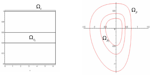
Figure 2: The subregion $\Omega_{c_{i}}$ in $\Omega_{c}$ is mapped into $\Omega_{p_{i}}$ in $\Omega_{p}$.

The new values of $s^{{}^{\prime}}_{ij}$ can be used to generate the new positions of the points on the grid lines since the piecewise linear representation of the underlying arc is available (Fig. 1b). For more details see [16]. A similar procedure is performed in the third stage along the horizontal grid curves, with the monitor in the  $x$ coordinate direction again (Fig. 1c).
The mesh resulting from the above procedure forms quadrilaterals whose sides equi-distribute the grid lines in the two coordinate directions (see Fig. 1c).

4 Adaptive nodes in a non-rectangular domain

In this section we present a new technique for generating adaptive nodes in a simply connected domain, $\Omega_{p}$, bounded by a closed curve $\Gamma$. For ease of explanation, we assume that $\Gamma$ can be given by the parametric equations

$$\Gamma:x=g_{1}(\theta),\quad y=g_{2}(\theta),\quad 0\leq\ \theta\leq 2\pi,$$

where $\theta$ is the angle used in the polar coordinate system and measured in the conventional anti-clockwise direction. The key to our proposed method is to make use of a rectangular transformation and to produce an adaptive mesh in the rectangle. We introduce a mapping

$$\psi:\Omega_{c}\rightarrow\Omega_{p}$$ (3)

where

$$\Omega_{c}=\{(\theta,r),0\leq\theta\leq 2\pi,\ 0\leq r\leq 1\}$$

is a rectangle in the cartesian coordinate system $(\theta,r)$, referred to as computational domain, $\Omega_{p}$ is the physical domain and the transformation is defined by the following functions

$$\left\{\begin{array}[]{l}x=rg_{1}(\theta),\\ y=rg_{2}(\theta).\end{array}\right.$$ (4)

One can easily see that the above transformation corresponds the line $r=1$ in $\Omega_{c}$ to the boundary $\Gamma$ in $\Omega_{p}$. In addition, any rectangular subregion $\Omega_{c_{i}}$ in $\Omega_{c}$ is mapped into a subregion $\Omega_{p_{i}}$ in $\Omega_{p}$ as shown in Fig. 2.
The method described in section 3 and used to produce grid points in a rectangle, is now applicable to the computational domain $\Omega_{c}$. Before explaining the adapting technique, we propose a method to construct a uniform mesh in $\Omega_{p}$ by the use of the transformation in (3).

We start with a uniform mesh in $\Omega_{c}$ in the cartesian coordinate system $\theta r$ as follows,

$$\theta_{0}<\theta_{1}<\dots<\theta_{n-1}=2\pi-h_{\theta},$$

$$h_{r}=r_{1}<r_{2}<\dots<t_{m-1}<r_{m}=1,$$

where

$$h_{\theta}=\frac{2\pi}{n},\ \theta_{j}=jh_{\theta},\ j=0,1,\dots,n-1,$$

and

$$h_{r}=\frac{1}{m},\ r_{i}=ih_{r},\ i=1,2,\dots,m.$$

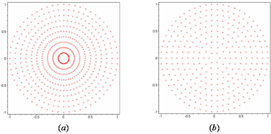
Figure 3: The mesh points transformed from $\Omega_{c}$ into a circle before and after refinement are displayed in Figures (a) and (b) respectively.

Using equations (4) the mesh points $(\theta_{j},r_{i})$ are transformed to the points $(x_{i},y_{j})$ in the $xy$ coordinate system, as depicted in Fig. 3. Unlike the mesh in $\Omega_{c}$, the new mesh in $\Omega_{p}$ is non-uniform, since each line $r=r_{i}$ in $\Omega_{c}$ corresponds to a closed curve in $\Omega_{p}$ with the same number of nodes, n. Therefore, the mesh will be clustered around the center, especially, for small values of $r$. This feature affects the quality of the grid points. To avoid this difficulty, below we suggest a refinement process to construct a roughly uniform mesh referred to as a uniform mesh in this paper. Although there might be some easier way to produce a set of uniform mesh points in an irregular region, the following method will be utilized in the adapting technique later.

4.1 A uniform mesh in $\Omega_{p}$

In order to obtain a uniform mesh in $\Omega_{p}$, we now refine the above mesh points obtained by the transformation. The refinement process is performed by modifying the number of nodes on each closed curve, $r=r_{i}$ based on a suitable criteria. For instance, we suggest this number of points to be selected in such away that the distance between the adjacent points on each closed curve be the same as that on the boundary. we propose the following process which is based on the perimeter of the closed curves.
The perimeter of the $i$th curve can be approximated by the perimeter of a circle whose radius is evaluated by the average length of the position vectors of the boundary points, i.e.

$$R_{i}=\frac{1}{n}\sum_{j=0}^{n-1}R_{ij},\ i=1,\dots,m,$$

where

$$R_{ij}=\sqrt{x^{2}_{ij}+y^{2}_{ij}},\ \ x_{ij}=r_{i}g_{1}(\theta_{j}),\ \ y_{ij}=r_{i}g_{2}(\theta_{j}).$$

The approximate number of nodes for the $i$th curve can be therefore obtained by

$$n_{\theta_{i}}=\frac{p_{i}}{\Delta s},$$ (5)

where $p_{i}=2\pi R_{i}$ is the perimeter of the circle and $\Delta s$ is the minimum distance between the adjacent boundary nodes. Another difficulty may arise due to the value of $n_{r}$. In fact, if the values of $n_{\theta}$ and $n_{r}$ are arbitrarily selected, the points may be clustered along the lines $\theta=\theta_{j}$ (see Fig. 4). To treat this issue we propose the value of $n_{r}$ to be selected based on $n_{\theta}$ using a criteria similar to the above mentioned process. For instance, for a given value of $n_{\theta}$, $n_{r}$ can be determined such that

$$\frac{p}{R}=\frac{n_{\theta}}{n_{r}},$$ (6)

where $p$ is the approximate perimeter of the boundary and $R$ is the average lengthes of the position vectors. A clustered and a refined mesh obtained by the above process are displayed in Figures 3a and 3b, respectively.
The suitably selected $n_{\theta_{i}}$ and $n_{r}$ will be also used in adapting mesh points later.

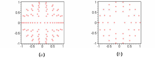
Figure 4: The points produced by an arbitrarily selected value of $n_{r}$ in (a) and a suitably selected value of $n_{r}$ based on relation (6) in (b) are displayed.

4.2 Adaptive nodes in non-rectangular regions

We now present a method to produce adaptive nodes in the physical domain $\Omega_{p}$. The key to this new approach is to make use of the adaptive mesh technique described in section 3 and the transformation (3). More precisely, some adaptive points are first prepared in the computational domain $\Omega_{c}$ and then transformed into the physical domain $\Omega_{p}$. Fig. 5 illustrates how, for instance, the third stage of adapting mesh in $\Omega_{c}$ is related to $\Omega_{p}$, i.e. equi-distributing along the grid lines for the coordinate $\theta$.

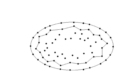
Figure 5: The grid curves in $\Omega_{p}$ resulted from the transformation of the grid lines in $\Omega_{c}$ in the third stage of adapting nodes.

Although, the mesh points produced by the above method is somehow adaptive, the concentration of the points around the center is an disadvantage as previously discussed. To overcome this difficulty, below we propose a refining mechanism in performing the 3-stage adaptive algorithm.
We start with a uniform mesh in $\Omega_{c}$ and perform the the first two stages of the adapting method. More precisely, the equi-distribution in the horizontal direction and the vertical grid lines are accomplished (Fig. 1a and 1b). But, the final stage is done in a different manner. We suggest a combination of the third stage of the adapting technique with the refinement process discussed in section 4.1 to avoid clustering the mesh points. As noted before, the density of the mesh around the center can be avoided by modifying the number of nodes along the closed curves. Recalling the refinement process to obtain a uniform mesh, a suitable number of points for the $i$th closed curve, $n_{\theta_{i}}$ was computed in (5). We can either use the same number of points or a new value of $n_{\theta_{i}}$ based on the new perimeter of the curves resulted from the first two stages.
Having obtained the horizontal grid lines by the two-stage procedure and found the $n_{\theta_{i}}$ for each curve, we can equi-distribute $n_{\theta_{i}}$ points along the horizontal grid curves used in the third stage of adapting method in Fig. 1c.

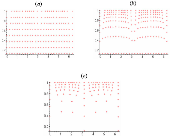
Figure 6: The illustration of the 3-stage adapting mesh in $\Omega_{c}$ with a refined number of nodes along each grid cure in the horizontal direction in (c) is displayed.

Fig. 6 illustrates the 3-stage adapting nodes in the rectangular domain. It is observed that in the third stage (Fig. 6c) a refined number of nodes, $n_{\theta_{i}}$ are distributed along the horizontal grid curves.

5 Meshless methods

In this section we first introduce the RBFs and then describe their application to the numerical solution of PDEs based on collocation meshless method.

5.1 Radial basis functions

RBFs are known as the natural extensions of splines to multi-variate interpolation. Suppose the set of points

$$\{x_{i}\in\Omega|i=1,2,\cdots,N\},$$

is given, where $\Omega$ is a bounded domain in $R^{n}$. The radial function $\varphi:\Omega\longrightarrow R$ is used to construct the approximate function

$$s(x)=\sum_{k=1}^{N}\alpha_{k}\varphi(\|x-x_{k}\|),$$

which interpolates an unknown function $f$ whose values at $\{x_{i}\}_{i=1}^{N}$ are known. $\|.\|$ represents the Euclidean norm. The unknown coefficients $\alpha_{k}$ are determined such that the following  $N$ interpolation conditions are satisfied,

$$f(x_{i})=s(x_{i})=\sum_{k=1}^{N}\alpha_{k}\varphi(\|x_{i}-x_{k}\|),\ \ \ i=1,\cdots,N.$$

There is a large class of interpolating RBFs [14] that can be used in meshless methods. These include the linear $1+r$, the polynomial $P_{k}(r)$, the thin plate spline (TPS) $r^{2}\log r$, the Gaussian $\exp(-r^{2}/\beta^{2})$, and the multi-quadrics $\sqrt{\beta^{2}+r^{2}}$ (with $\beta$ a constant parameter). In this paper we employ a generalized TPS, i.e. $r^{4}\log r$ which is a particular case of $r^{2k}\log r$ (k=2). These RBFs, augmented by some polynomials, are known as the natural extension of the cubic splines to the case of 2D. In fact, they are obtained by minimizing a $H^{m}$ semi-norm over all interpolants for which the semi-norm exists. The theoretical discussion of these RBFs has been presented in [9].

5.2 Collocation meshless method

We describe the collocation method for a general case of PDEs in the form

$$Lu=F,$$ (7)

where  $L=[L_{1},\cdots,L_{N}]^{T}$ represents a vector of linear operations and $F=[f_{1},\cdots,f_{N}]^{T}$ denotes a vector containing the right hand sides of the equations. For instance,  Poisson’s equation with a Dirichlet boundary condition

$$\begin{array}[]{cc}\Delta u=f,&\text{in}\ \Omega,\\ u=g,&\text{on}\ \partial\Omega,\\ \end{array}$$

is a very simple case of equation (7) where  $L=[\Delta,I]^{T}$,  $F=[f,g]^{T}$ and the operators $\Delta$ and $I$ act on the domain $\Omega$ and the boundary $\partial\Omega$ respectively.
The collocation method is simply to express the unknown function $u$ in terms of the $RBFs$ as

$$u(x)=\sum_{k=1}^{N}\alpha_{k}\varphi(\|x-x_{k}\|),$$ (8)

and determine the unknowns  $\alpha_{k}$  in such a way that (8) satisfies equation (7) for all interpolation points. Substituting (8) in equation (7) and imposing the  $N$ essential conditions of the collocation method lead to a linear system of equations whose coefficient matrix consists of  $N$ row blocks, the entries of which are of the form

$$A^{\mu}_{ij}=L_{\mu}\varphi(\|x-x_{j}\|)|_{x=x_{i}},\ \ \ i=1,\cdots,N_{\mu},\ j=1,\cdots,N,$$

where $N_{\mu}$ indicates the number of nodes associated with the operator $L_{\mu}$.
The above collocation method is referred to as a non-symmetric collocation method due to the non-symmetric coefficient matrices. The invertibility of the coefficient matrix can not be guaranteed [10], although in most cases a non-singular matrix is expected. To tackle this difficulty the symmetric collocation method, motivated by Hermitian interpolation, has been suggested. This method leads to symmetric matrices and proves the non-singularity of interpolation matrices at the expense of double acting the operators on the $RBFs$ [11]. Since this work is not concerned with the singularity of the matrices the non-symmetric case will be implemented. Of course, the main technique discussed in this paper can be applied to the other case as well.

6 Numerical Results

We now examine the effectiveness of the mesh generation technique by applying the collocation meshless method to some PDEs. In each case, the PDE is solved with some equally spaced nodes (roughly uniform) and adaptive nodes generated by the new method and the results are compared. As previously noted, $\phi(r)=r^{4}\log r$, is used as a basis function. In each example, $M$ test points, which do not coincide with the interpolation nodes, are randomly selected and a root mean square (RMS) error at these points is evaluated by

$$\text{RMS error}=\sqrt{\sum_{i=1}^{M}(u_{apr,i}-u_{ex,i})^{2}/M}$$

where $u_{apr,i}$ and $u_{ex,i}$ denote the approximate and exact values of $u$, respectively, at a test point $i$.

Equations (4) are used to evaluate the arc-length monitors

$$M_{\theta}=\sqrt{1+u_{\theta}^{2}}\ \ \ \text{and}\ \ \ M_{r}=\sqrt{1+u_{r}^{2}},$$

respectively for equi-distributing in the $\theta$ and $r$ coordinate directions where

$$u_{\theta}=\frac{\partial u}{\partial x}\frac{dx}{d\theta}+\frac{\partial u}{\partial y}\frac{dy}{d\theta},\ \ \ u_{r}=\frac{\partial u}{\partial x}\frac{dx}{dr}+\frac{\partial u}{\partial y}\frac{dy}{dr}$$

.

We consider the Poisson equation

$$\begin{array}[]{ll}\Delta u=f(x,y)&\text{in}\ \Omega\\ u(x,y)=g(x,y),&\text{on}\ \partial\Omega,\\ \end{array}$$ (9)

for different cases with various solutions and regions.

Example 1

We solve equations (9) in the case of

$$\begin{array}[]{l}f(x,y)=4e^{x^{2}+y^{2}}+4(x^{2}+y^{2})e^{x^{2}+y^{2}}\\ \\ g(x,y)=e^{x^{2}+y^{2}}\end{array}$$

and $\partial\Omega$ is an ellipse whose equation is $x^{2}+4y^{2}-1=0$.
In this case the exact solution is given by $u(x,y)=e^{x^{2}+y^{2}}$.

Table 1: Error values for Example 1

$n_{\theta},\ n_{r}$	25,4	31,5	37,6	43,7	50, 8	56,9	63,10	69,11
$n$	60	86	124	162	212	266	328	398
Adaptive	1.04E-3	8.47E-5	5.15E-5	2.31E-6	4.81E-6	5.14E-7	4.75E-7	7.67E-8
Uniform	2.53E-3	9.24E-4	3.42E-4	1.36E-4	5.57E-5	2.37E-5	1.09E-5	4.80E-6

Example 2

$$\begin{array}[]{l}f(x,y)=-4e^{(4-x^{2}-y^{2})}+4(x^{2}+y^{2})e^{(4-x^{2}-y^{2})}\\ \\ g(x,y)=e^{(4-x^{2}-y^{2})}\end{array}$$

and $\partial\Omega$ is the same as that in Example 1.
The exact solution is given by $u(x,y)=e^{(4-x^{2}-y^{2})}$.

Table 2: Error values for Example 2

$n_{\theta},\ n_{r}$	25,4	31,5	37,6	43,7	50, 8	56,9	63,10	69,11
$n$	60	86	124	162	212	266	328	398
Adaptive	3.055E-4	3.76E-4	1.42-4	6.32E-5	1.91E-5	7.23E-6	2.50E-6	8.43E-7
Uniform	2.89E-4	3.75E-4	2.26E-4	1.03E-4	4.32E-5	1.78E-5	7.83E-6	3.13E-6

Example 3

$$\begin{array}[]{l}f(x,y)=4\\ \\ g(x,y)=x^{2}+y^{2}\end{array}$$

and the boundary is given by the parametric equations:

$$\left\{\begin{array}[]{l}x=cos\theta\sqrt{1-cos\theta/2}\\ \\ y=sin\theta\sqrt{1-sin\theta/2}\\ \end{array}\right.$$

The exact solution is given by $u(x,y)=x^{2}+y^{2}$.

Table 3: Error values for Example 3

$n_{\theta},\ n_{r}$	25,4	30,5	45,8	55,9	65,11	75,12
$n$	60	78	142	262	366	460
Adaptive	1.13E-3	3.80E-5	2.54E-5	3.21E-6	3.80E-7	1.81E-7
Uniform	1.85E-3	7.62E-4	5.40E-5	2.27E-5	5.34E-6	2.46E-6

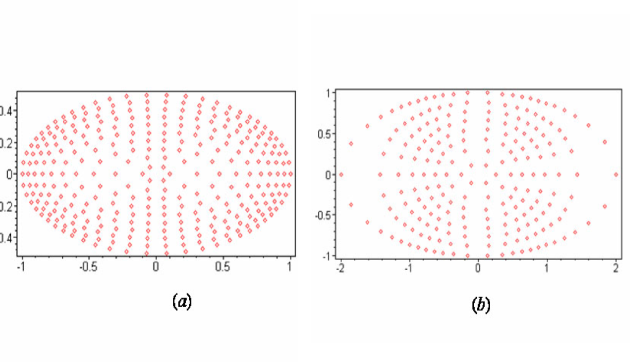
Figure 7: The adaptive nodes generated for the solutions of Examples 1 and 2 are displayed in (a) and (b) respectively.

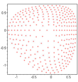
Figure 8: The adaptive nodes generated for the solution of Example 3.

The adaptive nodes generated for the above PDEs are displayed in Figures 7a, 7b and 8, respectively. One can expect, for the solution of Example 1, the mesh points to be more dense close to the boundary and, for the solution of Example 2, the mesh points to be more dense around the center. These are exactly what we observe in the figures. Therefore, the adaptive nodes are in a good agreement with the solutions. A similar situation is observed in Fig. 8 for the solution of Example 3.

The numerical errors for the above three examples are listed, respectively, in Tables 1, 2 and 3, where $n_{\theta}$ is the number of boundary points, $n$ is the total number of collocation points and $n_{r}$ is the appropriate number of divisions for the coordinate $r$ based on relation (6).
In all the examples, the numerical results demonstrate a considerable reduction in the error in the case of using the adapting nodes produced by the new adaptive method. In particular, Table 1 shows that the error in the case of using $398$ uniform nodes is nearly the same as that in the case of using $212$ adaptive nodes. Moreover, the error in the case of using $398$ uniform nodes is $63$ times larger than that in the case of using the same number of adaptive mesh points.

7 Conclusion

A new adaptive mesh technique was presented for irregular regions in two dimensional cases based on equi-distribution. The method was based on first, generating some adaptive nodes in a rectangle and then mapping the produced nodes to the physical domain using a suitable transformation.

The new method was examined by considering some PDEs solved by a collocation meshless method and the results demonstrated considerable reduction in the error values. Since the current work was not involved with constructing a monitor for the underlying method, a general monitor function, arc-length, was employed to produce the adaptive nodes. Of course, using a suitable monitor for the underlying method could have resulted in more improvement in the numerical results

The proposed method was implemented for 2D regions whose boundary was given by parametric equations in terms of polar coordinate system. For a more general case of irregular boundaries, we suggest a piecewise interpolation, in terms of some scattered points on the boundary, to make a set of parametric equations. Moreover, an extension of the new method to the case of 3D is currently under study and will be reported in a near future.

References

- [1] Beckett G., Mackenzie J. A., Ramage A. and Sloan D. M., On the numerical solution of one-dimensional PDEs using adaptive methods based on equi-distribution. Journal of Computational Physics, 167(2), 372-392, 2001.
- [2] Burgarellia D., Kischinhevskyb M., and Biezuner R. J., A new adaptive mesh refinement strategy for numerically solving evolutionary PDE’s . Journal of Computational and Applied Mathematics, 196(1), 115-131, 2006.
- [3] Cao W., Huang W. and Russell R. D., A study of monitor functions for two-dimensional adaptive mesh generation. SIAM J. Sci. Comput., 20(6), 1978-1994, 1999.
- [4] Carey G. F. and Humphrey D. L., Mesh refinement and iterative solution methods for finite element computations. Internat. J. Numer. Meth. Engng., 17(11), 1717-1734, 2005.
- [5] Chen C. S., Ganesh M., Golberg M. A. and Cheng A. H. D., Multi-level compact radial functions based computational schemes for some elliptic problems. Computers and Mathematics with applications, 43(3), 359-378, 2002.
- [6] Chen K., Two-dimensional adaptive quadrilateral mesh generation. Comm. Numer. Meth. Engng., 10(10), 815-825, 1994.
- [7] De Boor C., In good approximation by splines with variable knots II. Lecture notes Series 363, Springer-Verlag, Berlin, 1973.
- [8] Dubal M. R., Domain decomposition and local refinement for multi-quadric approximations I: Second-order equations in one-dimension. J. Appl. Sci. Comp., 1(1), 146-171, 1994.
- [9] Duchon J., Spline minimizing rotation-invariant semi-norms in Sobolev spaces In: W. Schempp, K. Zeller, eds. Constructive theory of function of several variables, lecture notes in mathematics 571, 85-100, Springer Berlin, 1977.
- [10] Fasshauer G. E., Solving partial differential equations with radial basis function: multi-level methods and smoothing. Advances in Computational Mathematics, 11, 139-159, 1999.
- [11] Fasshauer G. E., Solving partial differential equations by collocation with radial basis functions. In: Le Mehaute, A., Rabut C. and Schumaker LL. (eds.), Chamonix proceedings. Vanderbilt University Press, Nashville, TN, 1-8, 1996.
- [12] Kansa J., Multi-quadrics - a scattered data approximation scheme with applications to computational fluid dynamics-II. Comput. Math. Appl., 19(8/9), 147-161, 1990.
- [13] Kautsky J. and Nichols N. K., Equi-distributing meshes with constraints. SIAM J. Sci. Statist. Comput., 1(4), 449-511, 1980.
- [14] Powell M. J. D., The theory of radial basis function approximation in 1990, Advances in Numerical Analysis, vol. 2: Wavelets, Subdivision Algorithms and Radial Basis Functions, pp. 105 210, W.A. Light, ed., Oxford Univ. Press, 1992.
- [15] Ragusa J. C. and Wanga y., A two-mesh adaptive mesh refinement technique for SN neutral-particle transport using a higher-order DGFEM . Journal of Computational and Applied Mathematics 233, 3178-3188, 2010.
- [16] Shanazari K. and Chen K., A minimal distance constrained adaptive mesh algorithm with application to the dual reciprocity method. Numerical Algorithms, 32, 275-286, 2003.
- [17] Shanazari K. and Nima Rabie, A three dimensional adaptive nodes technique applied to meshless type methods Applied Numerical Mathematicss, 59, 1187-1197, 2009.
- [18] Shishkina O. and Wagner C., Adaptive meshes for simulations of turbulent Rayleigh-Benard convection. Journal of Numerical Analysis, Industrial and Applied Mathematics, 1(2), 219-228, 2006.
- [19] Sweby P. K., Data-dependent grids. Numerical Analysis Report 7/87, University of Reading, UK, 1987.
- [20] Wanga H. and Qing-Hua Q., A meshless method for generalized linear or nonlinear Poisson-type problems. Engineering Analysis with Boundary Elements, 30(6), 515-521, 2006.
- [21] Wendland H., Piecewise polynomial, positive definite and compactly supported radial function of minimal degree. Adv. Comput. Math., 4(1), 389-396, 1995.
- [22] White A. B., On selection of equi-distribution meshes for two-point boundary value problems. SIAM J. Numer. Anal., 16(3), 472-502, 1979.
- [23] Winslow A. M., Numerical solution of the quasi-linear Poisson’s equation in a non-uniform triangle mesh. J. Comput. Phys., 1(2), 149-172, 1967.
- [24] Zhang Y., Solving partial differential equations by meshless methods using radial basis functions. Applied Mathematics and Computation, 185, 614-627, 2007.