A Theoretical Study of the Equation of States for Crustal Matter of Strongly Magnetized Neutron Stars

Abstract

We have investigated some of the properties of dense sub-nuclear matter at the crustal region (both the outer crust and the inner crust region) of a magnetar. The relativistic version of Thomas-Fermi (TF) model is used in presence of strong quantizing magnetic field for the outer crust matter. The compressed matter in the outer crust, which is a crystal of metallic iron, is replaced by a regular array of spherically symmetric Wigner-Seitz (WS) cells. In the inner crust region, a mixture of iron and heavier neutron rich nuclei along with electrons and free neutrons has been considered. Conventional Harrison-Wheeler (HW) and Bethe-Baym-Pethick (BBP) equation of states are used for the nuclear mass formula. A lot of significant changes in the characteristic properties of dense crustal matter, both at the outer crust and the inner crust, have been observed.

1 Introduction

Magnetars are the most exotic stellar objects, believed to be strongly magnetized young neutron stars. The surface magnetic field for such objects are observed to be $\geq 10^{15}$G R1 ; R2 ; R3 ; R4 . Then it is quite likely that the field at the interior, even at the inner crust region may be stronger than the surface value (can be predicted theoretically by scalar Virial theorem). If the internal field strength is happened to be so high, then most of the physical and chemical properties of dense stellar matter of the magnetars must change significantly from the conventional picture R5 ; R6 ; R7 . A lot of investigations have already been done on the effect of strong quantizing magnetic field on various physical properties of dense stellar matter inside neutron stars as well as quark matter inside quark stars or hybrid stars, including the effect on quark-hadron phase transition at the core region of a compact neutron star R8 . The effect of such strong magnetic field on various elementary processes inside neutron stars and quark stars or hybrid stars have also been studied. The effect of strong quantizing magnetic field on the $\beta$-equilibration among the constituents have also been investigated R9 . It has also been shown that strong quantizing magnetic field acts like a catalyst to generate fermion mass dynamically, i.e., chiral symmetry breaking occurs in presence of strong quantizing magnetic field R10 ; R11 ; R12 .

In this article we present our investigation on the effect of strong magnetic field on the crustal matter of magnetars. The work is divided into two parts: in the first part, based on one of our very recent work R13 , we have investigated the effect of strong quantizing magnetic field on the outer crust matter. In the second part, we have studied the properties of compact sub-nuclear matter at the inner crust region in presence of such strong quantizing magnetic field.

The paper is organized in the following manner: In section 2, the effect of strong quantizing magnetic field on the crustal matter of magnetars is discussed. In the outer crust region, the matter with dense crystalline structure of metallic iron at sub-nuclear density are replaced by an array of spherically symmetric WS cells with positively charged nuclei at the centre surrounded by non-uniform dense electron gas with over all charge neutrality. In the inner crust we have used the conventional HW and BBP equation of states for the nuclear matter RR14 ; R14 ; R15 , consisting of iron along with some more heavier neutron rich nuclei. In one of our forth coming article we shall report the effect strong magnetic field on inner crust matter using some modern type nuclear mass formulas and make a comparative study with those models. Here we have presented with detailed numerical computation the effect of strong magnetic field on the inner crust matter, which as mentioned above is assumed to be a mixture of iron, some heavier neutron rich nuclei, which we found to be specially true in presence of strong quantizing magnetic field, electrons and free neutrons. The presence of free neutrons are considered beyond neutron drip density. Finally, in the last section, we have given the conclusions and discussed the importance and future prospects of the present work.

2 Crustal Matter

In the first part of this section, we present our study on the effect of strong magnetic field on the outer crust region with the composition mentioned in the introduction part. For a typical neutron star, the width of the outer crust region is $\sim 0.2-0.4$Km. In a recent work we have developed an exact formalism for the relativistic version of TF model in presence of strong quantizing magnetic field R13 . This formalism is used within the limitation of TF model R16 , to obtain the equation of state for crustal matter of a typical magnetar. In this model it has been assumed that for a WS cell, the atomic number is $Z$ and the mass number is $A$. To make each cell electrically charge neutral, $Z$ must also be the number of electrons inside the WS cells.

In this model, the modified form of Poisson’s equation is given by R13

$$\frac{d^{2}\phi}{dx^{2}}=\sum_{\nu=0}^{\nu_{\rm{max}}}(2-\delta_{\nu 0})(\phi^{2}(x)-\phi_{\nu}^{2}x^{2})^{1/2}$$ (1)

where $\phi(x)$ is the modified form of electrostatic potential related to the original Coulomb potential $V(x)$ by the relation

$$\phi(x)=\frac{\mu x}{Ze^{2}}[\mu_{e}+eV(x)],$$ (2)

with $\mu_{e}$, the electron chemical potential, assumed to be constant throughout the cell (this is the so called Thomas-Fermi condition), the dimensionless scaled radial coordinate $x$ is related to the actual radial coordinate $r$ of WS cells by the relation: $x=r/\mu$, with

$$\mu=\left(\frac{\pi}{2e^{3}B}\right)^{1/2},$$ (3)

$e=|e|$, the magnitude of electron charge, $B$ is the constant magnetic field, assumed to be along $z$-direction (we have chosen the gauge $A^{\mu}\equiv(0,0,xB,0)$),

$$\phi_{\nu}=\frac{m_{\nu}\mu}{Ze^{2}},$$ (4)

with $m_{\nu}=(m_{e}^{2}+2\nu eB)^{1/2}$, $m_{e}=0.5$MeV, the electron rest mass and $\nu=0,1,2,.......,\nu_{\rm{max}}$, is the Landau quantum number for the electrons, $\nu_{\rm{max}}$ is the upper limit of Landau quantum number (the upper limit of the Landau quantum number $\nu_{\rm{max}}$ is finite at zero temperature, otherwise $\nu_{\rm{max}}=\infty$). Finally, the factor $(2-\delta_{\nu 0})$ indicates that the zeroth Landau level is singly degenerate, whereas, all other states are doubly degenerate. In this article we have assumed that the electron gas in the dense crustal matter of crystalline metallic iron is strongly degenerate and is considered to be at zero temperature. Then it is quite obvious from the non-negative value of electron Fermi momentum, that the upper limit of Landau quantum number $\nu_{\rm{max}}$ is given by

$$\nu_{\rm{max}}=\frac{\mu_{e}^{2}-m_{e}^{2}}{2eB}$$ (5)

To obtain numerical solution for $\phi(x)$ for a given magnetic field and a particular set of $Z$ and $A$, we further assume that instead of a point object, the nucleus at the centre of a WS cell, has a finite dimension and is assumed to be spherical in nature, so that the corresponding radius $r_{n}=r_{0}A^{1/3}$, with $r_{0}=1.12$fm. Such a choice also removes the singularity problem of TF equation at the origin R17 . Therefore it is not necessary to implement the prescription given by Feynman, Metropolis and Teller to obtain the numerical solution for TF equation R18 . Again from the physics point of view, the potential must satisfy the boundary conditions, given by

$$rV(r)=Ze~{}~{}~{}{\rm{for}}~{}~{}~{}r\rightarrow r_{n},~{}~{}~{}{\rm{and}}~{}~{}~{}\frac{dV}{dr}=0~{}~{}~{}{\rm{for}}~{}~{}~{}r\rightarrow r_{s}$$ (6)

where $r_{s}$ is the radius of the WS cell. Then by simple algebraic manipulation it is easy to show that $\phi(x)$, the modified form of Coulomb potential satisfies the boundary conditions

$$\phi(x)|_{x=x_{n}}=1~{}~{}~{}{\rm{and}}~{}~{}~{}\frac{d\phi}{dx}|_{x=x_{s}}=\frac{\phi(x)}{x}|_{x=x_{s}},$$ (7)

where $x_{n}=r_{n}/\mu$, the scaled nuclear radius and $x_{s}=r_{s}/\mu$, the corresponding scaled radius of the WS cell. Both these quantities are dimensionless.

Further, the right hand side of the Poisson’s equation (eqn.(1)) must be real. Which requires $\phi_{\nu}x\leq|\phi(x)|$. This is an additional condition, to be satisfied by the upper limit of Landau quantum number, and may be written by the following inequality:

$$\nu_{\rm{max}}(x)\leq\left(\frac{e^{6}Z^{2}}{\pi x^{2}}\phi(x)^{2}-\frac{m_{e}^{2}}{2eB}\right),$$ (8)

From the definition of Landau quantum number, the above inequality must necessarily be $\geq 0$. The above equation also shows that the upper limit of Landau quantum number depends on the position ($x$ or $r$ coordinates) of the electron within the WS cell, with which it is associated.

Since electron distribution is non-uniform within each cell, the Fermi momentum of a particular electron must depend on its positional coordinate in the cell. Then it is expected that the variation of $p_{F}(r)$ will be such that the electron chemical potential, given by

$$\mu_{e}+eV(r)=(p_{F}(r)^{2}+m_{e}^{2}+2\nu(r)eB)^{1/2}$$

remain constant throughout the cell with proper space dependent Landau quantum number $\nu$.

Satisfying all these conditions, of which some of them are particularly necessary for this model, we have solved the Poisson’s equation numerically within the range of $r$ from nuclear surface to the WS cell boundary, for $B=B_{c}^{(e)},10\times B_{c}^{(e)},10^{2}\times B_{c}^{(e)}$ and $10^{3}\times B_{c}^{(e)}$, where $B_{c}^{(e)}$ is the quantum critical limit for the magnetic field at and above which the Landau levels are populated for the relativistic electrons, and may be expressed in terms of the universal constants, given by $eB_{c}^{(e)}=m_{e}^{2}$ (with the choice of unit $\hbar=c=1$). The magnetic field beyond this limit is called the quantizing magnetic field and the quantum mechanical effect plays an important role in this domain. The numerical value of this field is $4.43\times 10^{13}$G. Within the range $x_{n}\leq x\leq x_{s}$, the numerical solution for $\phi(x)$ can be fitted exactly by a straight line for a particular magnetic field strength $B$ and can be expressed as $\phi(x)=ax+b$. Obviously, the parameters $a$ and $b$ are functions of magnetic field strength. We have obtained this functional form by minimizing $\chi^{2}$ numerically using a computer code for multi-parameter fitting program. In Table-I we have shown the variation of the parameters $a$ and $b$ with magnetic field strength.

Because of some numerical in-accuracy, the values of the parameter $b$, the intersections of the straight lines with $y$-axis, are not exactly one. However, for all the magnetic field values, the parameter $b$ is very close to one. The numerical values for the other parameter $a$ is always negative and its magnitude increases with the increase in magnetic field $B$. Which actually means that the radius or the volume of a particular WS cell decreases with the increase in magnetic field strength. However, in this particular article, we have avoided the origin, considering a finite size nucleus of radius $r_{n}$ at the centre. Then we have on the nuclear surface $b=1-ar_{n}/\mu$. In Table-I we have also shown the explicit variation of $x_{s}$, the scaled surface radius of the WS cells, for various magnetic field strength. While solving the Poisson’s equation numerically for a given magnetic field strength $B$, the instruction is given in our numerical code to terminate if the surface condition, given by eqn.(7) is satisfied and hence we obtain $x_{s}$ (also $r_{s}=x_{s}\mu$) as a function of magnetic field strength. In fig.(1) we have shown the variation of $x_{s}$ and also the corresponding $r_{s}$ as given in eqn.(9) below, with the strength of magnetic field. This figure clearly shows that the WS cells become more compressed if the magnetic field becomes stronger. This is in some sense analogous to what is called the magnetostriction in classical magneto-statics. These two curves can also be fitted by the power law functions, given by

$$x_{s} = 29.43\times\left(\frac{B}{B_{c}^{(e)}}\right)^{-0.41}~{}~{}{\rm{MeV}}^{-1}~{}~{}{\rm{and}}~{}~{}~{}$$

$$r_{s} = 1.704\times\left(\frac{B}{B_{c}^{(e)}}\right)^{-0.91}~{}{\rm{\AA}}$$ (9)

Knowing the scaled Coulomb potential $\phi(x)$ at various $x$ points (in the range $x_{n}$ to $x_{s}$) within the WS cell for a given magnetic field strength, we have evaluated numerically $\nu_{\rm{max}}(x)$ at every $x$ points within the cell. The variations of $\nu_{\rm{max}}(x)$ with $x$ for four different magnetic field strengths are shown in fig.(2). Although $\nu_{\rm{max}}(x)$ must be a set of discrete numbers, for the sake of illustration, we have plotted it as a continuous variable. In this figure, curves $a$ and $b$ are for $B=B_{c}^{(e)}$ and $10\times B_{c}^{(e)}$ respectively. For these two curves, the variables $\nu_{\rm{max}}(x)$ is plotted along the left side $y$-axis and $x$ (this is actually $\mu x$ in Mev^-1) along $x$-axis at the bottom. Similarly for $B=50\times B_{c}^{(e)}$ and $100\times B_{c}^{(e)}$, the variations are shown by the curves $\alpha$ and $\beta$ respectively. In this case, $\nu_{\rm{max}}(x)$ is plotted along the right side $y$-axis and $x$ is plotted along upper $x$-axis. From this figure, it is possible to make a number of conclusions: (i) For larger $B$ values, $x_{s}$ are smaller. (ii) For smaller $B$, $\nu_{\rm{max}}(x)$ starts with quite large value near the nuclear surface, e.g., $=124$ and $=15$ as shown in curves $a$ and $b$ respectively. Whereas, for curve $\alpha$ it starts with $\nu_{\rm{max}}=2$ and for $\beta$, the starting value is $\nu_{\rm{max}}=1$. (iii) The discrete nature of $\nu_{\rm{max}}$ is obvious from the high magnetic field curves $\alpha$ and $\beta$. (iv) Finally, for all the field values, the upper limit $\nu_{\rm{max}}(x)$ becomes exactly zero at the surface of the WS cells. In other wards, we can say that all the electrons near the WS cell surface are strongly polarized and the spins are anti-parallel to the direction of magnetic field. This is, of course, a purely relativistic effect. The possibility of fully polarized scenario can easily be obtained from the analytical solution of Dirac equation for electrons in presence of strong quantizing magnetic field. The eigen functions will not be simple spinor solutions, whereas the energy eigen value will be $E_{\nu}=(p_{z}^{2}+2\nu eB+m_{e}^{2})^{1/2}$, with $2\nu=n+1+m_{s}$, where $n=0,1,2,..$ is the Landau principal quantum number and $m_{s}=\pm 1$, the eigen values for the spin operator $\sigma_{z}$ R19 ; R13 . Hence, for $\nu=\nu_{\rm{max}}=0$, the only possible choice is the combination $n=0$ and $m_{s}=-1$. Which actually means that in the zeroth Landau level the spins of all the electrons are in the direction opposite (this is due to negative charge carried by the electrons) to the external magnetic field. We have further noticed that beyond the field value $100\times B_{c}^{(e)}$ (which is slightly $>10^{15}$G), the upper limit $\nu_{\rm{max}}(x)$ becomes identically zero not only at the surface region of WS cells, but at all the points inside the cell.

To obtain the density distribution of electrons within the WS cells, let us consider the expression for electron number density, given by

$$n_{e}(x)=\frac{eB}{2\pi^{2}}\sum_{\nu=0}^{\nu_{\rm{max}}(x)}(2-\delta_{\nu 0})p_{F}(x)$$ (10)

where the electron Fermi momentum $p_{F}(x)$ can be obtained from the TF condition and is given by

$$p_{F}(x)=\left\{Z^{2}e^{4}\left(\frac{\phi(x)}{\mu x}\right)^{2}-m_{\nu}^{2}\right\}^{1/2}$$ (11)

Since the electron density is larger near the nuclear surface inside the WS cells compared to the boundary values, the effect of electron density dominates over the influence of magnetic field strength at the central region, whereas near the WS surface, the magnetic field will play significant role. This will naturally make the upper limit $\nu_{\rm{max}}$ large enough (except for $B\geq 10^{15}$G) near the nuclear surface and quite small or identically zero near WS cell boundary. The results are also quite obvious because of the electron Fermi momentum, which is minimum at the nuclear surface and maximum near the the WS cell boundary. Later we shall show that the electron kinetic energy will also behave like Fermi momentum. Therefore. the quantum mechanical effect for low and moderate values magnetic field strength will be more significant near the surface region compared to the core region, where the effect is almost classical. This is particularly obvious from the curves $a$ and $b$ of fig.(2). For these curves, $\nu_{\rm{max}}(x)$ is naturally started with quite large values.

Using the numerically fitted form of $\phi(x)$ we obtain $p_{F}(x)$ for a given magnetic field strength and the corresponding $n_{e}(x)$. In fig.(3) we have plotted the variation of electron density within WS cells for four different magnetic field strengths. In this figure, the curves indicated by the numbers $0,1,2$ and $3$ are for $B=B_{c}^{(e)}$, $B=10\times B_{c}^{(e)}$, $B=10^{2}\times B_{c}^{(e)}$ and $B=10^{3}\times B_{c}^{(e)}$ respectively. The physical reason behind such increase in electron density is because of the decrease in WS cell volume with the increase in magnetic field strength, whereas, the total amount charge within the cell remain constant. It is quite obvious from these curves that the electron density increases with the increase in magnetic field strength. Further, for all the values of $B$, electron density is maximum at the centre and minimum at the surface. The oscillatory nature of $n_{e}(x)$ is because of the crossing of various Fermi levels within the cell. This is a kind of de Haas van Alphen effect. In our model we have assumed eqn.(10) as given in R13 . One must use the condition LY

$$\epsilon_{e}(r)-eV(r)+E_{ex}(r)=\mu_{e}=~{}~{}{\rm{constant}}~{}~{}$$ (12)

then re-cast the differential equation as given by eqn.(1) in this article. Here $E_{ex}$ is the electron-electron exchange energy per particle. However, with this choice it will be an almost impossible task to solve the problem even numerically. Hence we have made approximation by using eqn.(10) of R13 .

Let us now evaluate the variation of (i) electron kinetic energy, (ii) electron-nucleus interaction energy, (iii) electron-electron direct interaction energy and (iv) electron-electron exchange energy within the WS cells. The kinetic energy part for electrons at a particular point ($r$) within the WS cell is given by

$$E_{KE}(x) = \int_{r_{n}}^{r}d^{3}r\frac{eB}{2\pi^{2}}\sum_{\nu=0}^{\nu_{\rm{max}}(r)}(2-\delta_{\nu 0})$$ (13)

$$\int_{0}^{p_{F}(r)}dp_{z}[(p_{z}^{2}+m_{\nu}^{2})^{1/2}-m_{e}]$$

Evaluating the integral over $p_{z}$ analytically and then substituting for $p_{F}(x)$ from eqn.(11), with the numerically fitted functional form of $\phi(x)$, one can obtain the electron kinetic energy $E_{KE}$, as a function of $r$ or $x$ by the numerically evaluating the above integral. We have seen that within the WS cells, for constant $B$, the kinetic energy part satisfies a power law of the form $E_{KE}=\alpha x^{\beta}$, where the parameters $\alpha$ and $\beta$ are functions of magnetic field strength. In Table-I we have shown these variations. The change is more significant for $\alpha$ than $\beta$. Therefore, just like the electron density, the electron kinetic energy is also an increasing function of radial coordinate $x$ but does not show oscillation.

Next we consider the three possible types of interaction potential. Let us first consider the electron-nucleus interaction part, given by R13

$$E_{en}(r)=-Ze^{2}\int_{r_{n}}^{r}d^{3}r\frac{n_{e}}{r}$$ (14)

$$= -4\pi Ze^{2}\mu^{2}\int_{x_{n}}^{x}xdxn_{e}(x)$$

To obtain this quantity within the WS cell for a constant $B$, we substitute the expression for electron number density $n_{e}(x)$ from eqn.(10), and then numerically integrate over $x$ In fig.(4) we have shown the variation of $-E_{en}(x)$ (which is a positive quantity) as a function of $x$ within the WS cell for three different magnetic field strengths: $B=B_{c}^{(e)},10^{2}\times B_{c}^{(e)}$ and $10^{3}\times B_{c}^{(e)}$. For very low $x$ values, i.e., almost on the surface of the nucleus at the centre, the magnitude of the potential energy is an increasing function of $x$, which actually means that the region is strongly attractive in nature. Again at the surface region, just at the skin of the cell, it is again an increasing function of $x$ (with larger gradient), so that the attractive field again becomes extremely strong at the surface region to keep the outer most electrons confined within the cell. At the middle region, there is a kind of saturation and force due to electron-nucleus interaction almost vanishes. This is quite analogous to the normal metallic scenario, in which electric field can not exist.

Next we consider the electron-electron interaction. Let us first evaluate the direct term. It is given by R13

$$E_{ee}^{(d)}=\frac{1}{2}e^{2}\int d^{3}rn_{e}(r)\int d^{3}r^{\prime}n_{e}(r^{\prime})\frac{1}{|\vec{r}-\vec{r^{\prime}}|}$$ (15)

Assuming $\vec{r}$ as the principal axis and $\theta$ is the angle between $\vec{r}$ and $\vec{r^{\prime}}$, we have $d^{3}r~{}=~{}4\pi~{}r^{2}~{}~{}dr$,
$d^{3}r^{\prime}=2\pi{r^{\prime}}^{2}dr^{\prime}\sin\theta d\theta$ (we have assumed that the vectors $\vec{r}$ and $\vec{r^{\prime}}$ are on the same plane) and $|\vec{r}-\vec{r^{\prime}}|=(r^{2}+{r^{\prime}}^{2}-2rr^{\prime}\cos\theta)^{1/2}$. The limits for both $r$ and $r^{\prime}$ are from $r_{n}$ to $r_{s}$ and the range of $\theta$ is from $0$ to $\pi$. Then evaluating the trivial integral over $\theta$ the direct interaction, part reduces to the following simple form:

$$E_{ee}^{(d)} = 8e^{2}\pi^{2}\Big{\{}\int_{r_{n}}^{r}rdrn_{e}(r)\int_{r_{n}}^{r}{r^{\prime}}^{2}dr^{\prime}n_{e}(r^{\prime})$$ (16)

$$+ \int_{r_{n}}^{r}r^{2}drn_{e}(r)\int_{r}^{r_{s}}r^{\prime}dr^{\prime}n_{e}(r^{\prime})\Big{\}}$$

Following the same procedure adopted for $E_{en}$ case, we have evaluated numerically the above coupled integrals. In fig.(5) we have shown the variation of $E_{ee}^{d}(x)$ within the WS cell for three different magnetic field strengths: $B=B_{c}^{(e)},10^{2}\times B_{c}^{(e)}$ and $10^{3}\times B_{c}^{(e)}$. Surprisingly, the variations are almost identical with $|E_{en}|$. However, the magnitudes are several orders less than the corresponding electron-nucleus part. Of course, unlike the $E_{en}$, the direct term is positive throughout and for all the values of magnetic field strength. The same kind of qualitative nature of $\mid E_{en}\mid$ and $E_{ee}^{(d)}$ (figs.(4)-(5)) makes the system of electron gas within the WS cell energetically stable. Of course the kinetic energy part and the exchange part also play important role. The combination of kinetic energy and three interaction potentials of which electron-nucleus interaction part and the exchange part are negative, gives a constant energy for a particular electron at any point within the WS cell. This constant energy is the electron chemical potential and is also the minimum possible energy at a particular point.

Next we shall consider the exchange term, which is negative in nature. The magnitude of exchange energy integral corresponding to the $i$th. electron in the cell is given by R13

$$E_{ee}^{(ex)}=\frac{e^{2}}{2}\sum_{j}\int d^{3}rd^{3}r^{\prime}\frac{1}{|\vec{r}-\vec{r^{\prime}}|}\bar{\psi}_{i}(\vec{r})\bar{\psi}_{j}(\vec{r^{\prime}})\psi_{j}(\vec{r})\psi_{i}(\vec{r^{\prime}})$$ (17)

where the spinor wave function $\psi(\vec{r})$ is given by eqns.(2)-(5) in R13 and $\bar{\psi}(\vec{r})=\psi^{\dagger}(\vec{r})\gamma_{0}$, the adjoint of the spinor and $\gamma_{0}$ is the zeroth part of the Dirac gamma matrices $\gamma_{\mu}$. Now it is very easy to show that for $t=t^{\prime}$

$$\bar{\psi}_{i}(\vec{r})\psi_{i}(\vec{r^{\prime}})=\frac{2m}{L_{y}L_{z}E_{\nu}}\exp[-i\{p_{y}(y-y^{\prime})+p_{z}(z-z^{\prime})\}]$$

$$\{I_{\nu;p_{y}}(x)I_{\nu;p_{y}}(x^{\prime})+I_{\nu-1;p_{y}}(x)I_{\nu-1;p_{y}}(x^{\prime})\}$$ (18)

Similarly, we have

$$\bar{\psi}_{j}(\vec{r^{\prime}})\psi_{j}(\vec{r})=\frac{2m}{L_{y}L_{z}E_{\nu}^{\prime}}\exp[i\{p_{y}^{\prime}(y-y^{\prime})+p_{z}^{\prime}(z-z^{\prime})\}]$$

$$\{I_{\nu^{\prime};p_{y}^{\prime}}(x)I_{\nu^{\prime};p_{y}^{\prime}}(x^{\prime})+I_{\nu^{\prime}-1;p_{y}^{\prime}}(x)I_{\nu^{\prime}-1;p_{y}^{\prime}}(x^{\prime})\}$$ (19)

where $I_{\nu;p_{y}}(x)$ is same as $I_{\nu}$, given by eqn.(5) in R13 . When these two terms are combined, we have, after replacing the sum over $j$ by the integrals

$$L_{y}L_{z}\int_{-\infty}^{+\infty}dp_{y}^{\prime}\int_{-p_{F}}^{+p_{F}}dp_{z}^{\prime}$$

$$E_{ee}^{(ex)}=\left(\frac{e^{2}}{2}\right)\left(\frac{4m^{2}}{L_{y}^{2}L_{z}^{2}E_{\nu}}\right)\sum_{\nu^{\prime}=0}^{\nu_{\rm{max}}}(2-\delta_{\nu^{\prime}0})$$

$$\int...\int L_{y}dp_{y}^{\prime}L_{z}dp_{z}^{\prime}d^{3}rd^{3}r^{\prime}\frac{1}{E_{\nu^{\prime}}}\frac{1}{|\vec{r}-\vec{r^{\prime}}|}$$

$$\exp[-i\{(p_{y}-p_{y}^{\prime})(y-y^{\prime})+(p_{z}-p_{z}^{\prime})(z-z^{\prime})\}]$$

$$[\{I_{\nu;p_{y}}(x)I_{\nu;p_{y}}(x^{\prime})+I_{\nu-1;p_{y}}(x)I_{\nu-1;p_{y}}(x^{\prime})\}$$

$$\{I_{\nu^{\prime};p_{y}^{\prime}}(x)I_{\nu^{\prime};p_{y}^{\prime}}(x^{\prime})+I_{\nu^{\prime}-1;p_{y}^{\prime}}(x)I_{\nu^{\prime}-1;p_{y}^{\prime}}(x^{\prime})\}]$$ (20)

It is possible to evaluate the integrals over $y^{\prime}$ and $z^{\prime}$, given by R20

$$\int_{-\infty}^{+\infty}\int_{-\infty}^{+\infty}dy^{\prime}dz^{\prime}\frac{1}{|\vec{r}-\vec{r^{\prime}}|}$$ (21)

$$\exp[-i\{(p_{y}-p_{y^{\prime}})(y-y^{\prime})+(p_{z}-p_{z^{\prime}})(z-z^{\prime})\}]$$

$$= \frac{4\pi}{2K}\exp(-K|x-x^{\prime}|)$$

where $K=[(p_{y}-p_{y^{\prime}})^{2}+(p_{z}-p_{z^{\prime}})^{2}]^{1/2}$. Further, the integral over $y$ and $z$ is given by

$$\int_{-\infty}^{+\infty}\int_{-\infty}^{+\infty}dydz=L_{y}L_{z}$$

Since the final form of exchange integral is multidimensional in nature with an extremely complicated structure of integrand, it is absolutely impossible to have analytical solution for $e-e$ exchange potential. We have therefore adopted the multi-dimensional Monte-Carlo integration code to evaluate the exchange term. It is found that the variation of the magnitude of exchange energy with the scaled radius $x$ within the WS cells for a constant $B$ can be expressed by the power law formula, given by

$$\mid E_{ee}^{(\rm{ex})}\mid=px^{q},$$

where the parameters $p$ and $q$ are again functions of magnetic field strength $B$. The variation of the parameters $p$ and $q$ with magnetic field are shown in Table-I.

From the variation of the parameters $p$ and $q$ with $B$, it is quite clear that the magnitude of exchange energy also increases with $x$ and also with the magnetic field strength $B$, i.e., minimum at the central nuclear surface and maximum at the WS cell boundary.

The overall pressure term can also be obtained for the electron gas from the total energy $E_{\rm{tot}}$, given by

$$P(x)=n_{e}^{2}(x)\frac{\partial E_{tot}}{\partial n_{e}}=P_{k}(x)+P_{c}(x)$$ (22)

where

$$P_{k}=\frac{eB}{2\pi^{2}}\sum_{\nu=0}^{\nu_{\rm{max}}}(2-\delta_{\nu 0})\int_{0}^{p_{F}}\frac{p_{z}^{2}}{(p_{z}^{2}+m_{\nu}^{2})^{1/2}}dp_{z},$$ (23)

is the electron kinetic pressure part. The momentum integral for the kinetic pressure can very easily be obtained, and is given by

$$P_{k} = \frac{eB}{2\pi^{2}}\sum_{\nu=0}^{\nu_{\rm{max}}}(2-\delta_{\nu 0})\Big{[}p_{F}(p_{F}^{2}+m_{\nu}^{2})^{1/2}-$$ (24)

$$m_{\nu}^{2}\ln\left(\frac{p_{F}+(p_{F}^{2}+m_{\nu}^{2})^{1/2}}{m_{\nu}}\right)\Big{]}$$

Since $p_{F}=p_{F}(x)$, this expression will give the electron kinetic pressure at various points within the WS cell. The other term, $P_{c}$, coming from the interaction part, $E_{c}=E_{en}+E_{ee}^{(d)}+E_{ee}^{(ex)}$, and is given by

$$P_{c}(x)=n_{e}^{2}(x)\frac{\partial E_{c}}{\partial n_{e}},$$ (25)

The interaction part of electron pressure is obtained numerically by substituting the expression for $p_{F}(x)$ and evaluating the derivatives over $n_{e}$ numerically for a given $B$, at a particular point $x$ within the cell and also for a given set of $A$ and $Z$. We have noticed that at the central region of WS cells, since the density dominates over the magnetic field part, the total pressure is positive, while at the outer end, the surface region, since magnetic field dominates over the density contribution, it becomes negative. It is found numerically that at some point within the WS cell for a given $B$, the total pressure becomes exactly zero. It is found that this critical position is a function of magnetic field strength and decreases with the increase in magnetic field strength. In fig.(6) we have plotted this variation. The functional dependence can also be expressed as

$$x_{c}=\alpha+\beta\exp\left[-\gamma\frac{B}{B_{c}^{(e)}}\right]~{}~{}{\rm{MeV}}^{-1}$$ (26)

with $\alpha=0.38$, $\beta=1.28$ and $\gamma=0.171$. If the quantum mechanical effect of strong magnetic field dominates over the density effect, electrons either occupy only the zeroth Landau level or low lying levels. Which further causes a decrease in pressure term. As the magnetic field becomes strong enough, the density effect vanishes, even near the centre, which makes $x_{c}$ extremely small.

In the second part of this section we shall study the effect of strong quantizing magnetic field on inner crust matter at sub-nuclear density. In the conventional neutron star model, for a typical neutron star of radius $\approx 10$km, the width of inner crust is about $0.5-0.6$km. It is also believed that the free neutrons in the inner crust region may be in super-fluid state. The density range of this zone depends on the type of equation of state or the mass formula for the heavy nuclei, including the highly neutron rich nuclei. The density range in the conventional picture is $\sim 10^{9}-10^{12}$g/cm³. To investigate the properties of inner crust matter, here also we replace the metallic iron atoms and other heavier atoms with neutron rich nuclei, by WS cells as has been done for the outer crust matter. We further assume that the free neutrons in this region, above the neutron drip point are in normal fluid state.

In this part, to study the effect of strong quantizing magnetic field on inner crust matter, we consider two types of conventional nuclear mass formulae, which are generally used below the nuclear saturation density, but applicable near neutron drip region. These two mass formulae are (i) Harrison-Wheeler (HW) equation of state, and (ii) Bethe-Baym-Pethick (BBP) equation of state RR14 ; R14 ; R15 . We have already mentioned that in a future communication the effect of strong magnetic field on the equation of states with more modern type nuclear mass formulas will be reported.

In HW equation of state, the relativistic electrons are assumed to be in $\beta$-equilibrium with the nuclei (which also includes the neutron rich nuclei). Whereas, above the neutron drip density, the $\beta$-equilibrium is among the nuclei, free neutrons and the electrons. We have noticed that the presence of a strong quantizing back ground magnetic field modifies the $\beta$-equilibrium configuration significantly although we have assumed that the electrons are only affected by the presence of strong magnetic field. As a consequence of which more heavier neutron rich nuclei are produced in presence of strong magnetic field in the inner crust region. In the conventional astrophysical scenario, in presence of free electron gas in stellar medium, the balance between Coulomb force and the nuclear force, which gives ${}^{56}Fe$ as the most stable nucleus will get shifted towards the heavier nuclei. The nuclei, formed in such an environment will contain more neutrons (by inverse $\beta$-decay) compared to the usual picture. The Coulomb force plays a very little role. The nuclei becomes more and more neutron rich as the electron density goes up and when the matter density increases to $\sim 4\times 10^{11}$g/cm³, the ratio $n/p$ reaches a critical level. Any further increase in density will lead to neutron drip in the medium. In such a scenario, highly neutron rich nuclei, electrons and free neutrons co-exist in chemical ($\beta$) equilibrium. With the further increase in matter density, beyond neutron drip, nuclei, including the heavier ones melt and free neutrons appear in the medium and at some stage the kinetic pressure of the system will be dominated by the free neutron pressure instead of electron pressure which may become negative if the magnetic field is strong enough. We shall see later that this positive pressure contribution of free neutrons make the total pressure within the inner crust region a positive definite, even in presence of strong magnetic field. Whereas in the outer crust, the total pressure, coming from the electron gas only and is negative at the surface region of WS cells in presence of strong magnetic field.

The BBP equation of state is applicable for nuclear matter in the density range from neutron drip density $\rho_{\rm{drip}}$ to normal nuclear density $\rho_{\rm{nuc.}}$ ($\sim 2.8\times 10^{14}$g cm^-3). It is well known that BBP equation of state is a considerable improvement over the HW equation of state. In BBP equation of state, a mass formula, more or less like the HW equation of state is used but incorporated a lot of improvements from detailed many body calculation. The nuclear surface energy, for example, assumed in the previous treatment to be that of a nucleus in vacuum. An introduction of free neutron gas out side the nuclei reduces the nuclear surface energy. This is quite correct, because when inside and out side of a nuclei become identical, the surface energy must vanish. In BBP equation of state, the nuclear Coulomb energy is included in a more accurate manner and is called nuclear lattice Coulomb energy. It is well known that the BBP equation of state is applicable up to nuclear density, therefore, when all the bound nuclei dissolves into a continuous matter, mainly composed of free neutrons and a tiny fraction of protons and electrons, to incorporate this type of melting process of nuclei, in the BBP equation of state the factors giving the fractional volume occupied by the nuclei and the fractional volume occupied by the free neutron gas have been taken into account. It is also assumed that at this density ($<\rho_{\rm{nuc.}}$) the nuclei are stable to $\beta$-decay. Further, the neutrons in the free neutron gas are in chemical equilibrium with the electrons and the nucleons within the nuclei and in addition to the $\beta$-stability of the nuclei, the whole system must be in chemical equilibrium. In this model the kinetic pressure of free neutrons must necessarily be equal with the pressure of the nucleons bound within the nuclei. This is the condition for mechanical equilibrium. Since detailed mathematical formalism for both HW and BBP equation of states, which are assumed to be not affected by strong magnetic fields, are available in a large number of classic papers, including the original ones, and also included in many standard text books RR14 ; R14 ; R15 . The effect of strong quantizing magnetic field on the electron part has already been discussed in the previous section. In this section, we therefore present only the numerical results based on these two equation of states along with the results related to electron gas where ever needed, as developed in the first part of this section.

In the numerical computation, we have found that for very low mass number, since there is no free neutrons available in the system, even much above the neutron drip density, only electrons contribute in total kinetic pressure and is negative if the magnetic field affects the electron part quantum mechanically. This result is almost identical with the outer crust scenario. In fig.(7) we have plotted the variation of the critical value of mass number $A$ and the corresponding atomic number $Z$ with the strength of magnetic field using HW and BBP equation of states, These are the critical values at which the kinetic pressure of the inner crust region just becomes zero, i.e., the system just becomes mechanically stable. It is obvious from this figure that the minimum of mass number of the nuclei for which the inner crust matter just becomes mechanically stable, increases with the strength of magnetic field. In other words, this is equivalent to say that the presence of strong magnetic field makes the nuclei more and more massive or increases the minimum mass of the nuclei in the inner crust region. In some of our previous work, done long ago R12 , we have seen that the same conclusion is applicable for quark matter. The presence of strong quantizing magnetic field generates quark mass dynamically in dense quark matter composed of massless quarks. This is the well known magnetic field induced chiral symmetry violation. The strong quantizing magnetic field acts like a catalyst to generate / increase mass. In the BBP equation of state the minimum mass of the nuclei are more than that obtained from HW equation of state. Further, one should notice from this figure (figs.(7)) that for low and moderate strength of magnetic field, the effect is not so significant. But beyond $10^{15}$G, when all the electrons occupy the zeroth Landau level, or in other words, when the quantum mechanical effect of strong magnetic field is most important, the minimum mass rises sharply to very large values. One can see from R12 that the qualitative nature of the curve showing the dependence of dynamical quark mass on the magnetic field strength is exactly identical, although the physical scenarios are completely different.

In fig.(8), we have plotted the variation of the ratio $n_{e}/n$ and $n_{n}/n$ with the mass number using HW equation of state. Here $n_{e}$ is the electron density, $n_{n}$ is the free neutron density and $n=n_{n}+n_{e}A/Z$ is the total baryon density of inner crust matter. Dashed curve is for $B=0$, middle and the lower curves, indicated by $e1$ and $e2$ are for $B=10^{2}B_{c}^{(e)}$ and $10^{3}B_{c}^{(e)}$ respectively. The curve indicated by $n$ is for free neutron gas. In the HW equation of state, the neutron number density above the neutron drip point is independent of magnetic field strength. Further, the mass number around which neutrons are liberated from neutron rich nuclei is about $95$, which is again independent of magnetic field strength. However, immediately after the emission of neutrons from heavy neutron rich nuclei the overall kinetic pressure can not become non-zero. In fig.(9), we have plotted the same kind of variations as shown in fig.(8). Here we have used the BBP equation of state. Solid curves are for $B=0$, while the dashed curves are for $10^{3}B_{c}^{(e)}$. In this case the neutron drip out from heavy neutron rich nuclei around $A=100$, which is little bit heavier and more neutron rich than the HW case. Further, the qualitative nature of $x_{n}=n_{n}/n$ is totally different from HW case. Instead of increase initially and then saturates, as we observe in HW case, it decreases monotonically with A. Also, the free neutron density depends on the strength of magnetic field. However, the dependence is not so significant. These qualitative differences are found to be the consequence of chemical equilibrium among the free neutrons, electrons and nucleons within the heavy neutron rich nuclei and the overall $\beta$-equilibrium condition.

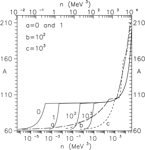
Figure 10: Variation of mass number of the nuclei with the total baryon density. HW equation of state: four different magnetic field strengths:$B=0$, $B=10B_{c}^{(e)}$, $B=10^{2}B_{c}^{(e)}$ and $B=10^{3}B_{c}^{(e)}$, indicated by $0$, $1$, $10^{2}$ and $10^{3}$ respectively. BBP equation of state: Dashed curves, the magnetic field strengths $B=0$, $B=10B_{c}^{(e)}$ (both are indicated by $a$), $B=10^{2}B_{c}^{(e)}$ (indicated by $b$) and $B=10^{3}B_{c}^{(e)}$ (indicated by $c$). Here, the lower x-axis is for HW equation of state and the upper one is for BBP equation of state.

In fig.(10). the variation of total nuclear density is plotted against the mass number for both HW and BBP equation of states. For the HW case, four different curves with magnetic field strengths: $B=0$, $B=10B_{c}^{(e)}$, $B=10^{2}B_{c}^{(e)}$ and $B=10^{3}B_{c}^{(e)}$ are indicated in the diagram by $0$, $1$, $10^{2}$ and $10^{3}$ respectively and shown by solid lines. In HW model, initially for low $A$ values, only the bound nucleons within the nuclei ($=An_{e}/Z$) contributes. Just beyond the critical value, $A=95$, since neutrons drip out from the heavy neutron rich nuclei, the number density jumps suddenly. Of course, below $A=60$, we can not have stable inner crust matter. The same kind of variation for BBP equation of state are shown by the dashed curves and indicated by the symbols $a$, $b$ and $c$. In this case, again because of chemical equilibrium conditions, the qualitative and the quantitative nature of the curves are completely different.

The equation of state from both HW and BBP mass formulas are plotted in fig.(11). From these two figures it is quite obvious that in presence of strong quantizing magnetic field, the inner crust matter becomes mechanically stable only at very high density, when enough number of free neutrons are available in the system. In this high density situation positive neutron kinetic pressure dominates over negative electron pressure in presence of strong quantizing magnetic field. This is true for both HW and BBP equation of states. Further, it is also obvious from the figures, that the matter becomes softer with the increase in magnetic field strength. The qualitative nature of both the equation of states are almost identical in presence of strong magnetic field. However, the HW equation of state is a bit softer than the BBP case.

3 Conclusions

In the first part of this article we have presented our investigation on the properties of dense outer crust matter of the magnetars. We have replaced the dense metallic iron crystal by a regular array of spherically symmetric WS cells. It has been observed that the radius of each cell decreases with the magnetic field strength. In this article, however, we have not considered the magnetic field induced deformation of WS cells, which is quite likely if the magnetic field is strong enough. In future we shall present this important issue with a completely different approach.

It has also been noticed that the upper limit of Landau quantum number is a function of positional coordinate of the electron with which it is associated within the WS cells. We have observed that at the surface region, for all the values of magnetic field strength, this upper limit becomes identically zero. Which actually means that the electrons near the WS cell surface are strongly polarized in the opposite direction of external magnetic field. Whereas, for $B>10^{15}$G, they are polarized at every points within the cells.

It has been observed that the electron density within the cells increases with the increase in magnetic field strength. Further, for all the values of magnetic field strength, the electron density is maximum near the nuclear surface ($r=r_{n}$) and minimum at the WS cell boundary ($r=r_{s}$).

The electron kinetic pressure is found to be positive near the central portion of WS cell but is negative near the surface region. There is a position within the cell at which the kinetic pressure vanishes. The position of this point changes with the strength of magnetic field. We have also studied the variations of kinetic energy, electron-nucleus interaction energy, electron-electron direct potential energy and electron-electron exchange interaction part within the cells. We have shown the variation of these quantities within the WS cells for a number of magnetic field strengths.

In the second part of this work, we have investigated some of the properties of inner crust matter of magnetars. We have used HW and BBP equation of states for the nuclear mass formula. It has been observed from both the models, that for a stable inner crust matter, the nuclei present must be heavier than iron and much more neutron rich. The heaviness is more in the case of BBP equation of state. We have also noticed that for low and moderate values of magnetic field strength, the variation of mass number and the corresponding atomic number with magnetic field is not so significant. Whereas, for $B\geq 10^{15}$G, when electrons occupy only the zeroth Landau level, then much more heavier neutron rich nuclei are formed in the inner crust region. It is found that high magnetic field behaves like a catalyst to generates heavy neutron rich nuclei.

We have observed that initially the electron density increases with the increase in mass number, but as soon as free neutrons appear in the system, the electron density decreases and saturates to some constant value which depends on the magnetic field strength. In the case of HW equation of state, free neutron density does not depend on the strength of magnetic field, whereas, for BBP case, because of chemical equilibrium condition, the free neutron density depends very weakly on the magnetic field strength. We have noticed that in the case of BBP equation of state the overall qualitative difference is because of chemical equilibrium among the constituents.

The total baryon density rises sharply like an avalanche for the value of $A$ at which free neutrons appear in the system. However, for BBP equation of state, because of chemical equilibrium condition, the rise is not so sharply visible for a given magnetic field $B$.

The qualitative nature of equation of states are almost identical. It is found that in presence of strong magnetic field, the inner crust matter becomes mechanically stable (with the positive value of kinetic pressure) only at very high density.

We therefore believe that to study various properties of dense matter associated with magnetars, one must consider all these significant changes from the conventional scenario. Further, we expect that the strong magnetic field, if present well within the inner crust of magnetars, must affect the super-fluidity of cold neutron matter.

Table 1: Variation of the parameter $a$ and $b$ for $\phi(x)=ax+b$ and scaled surface radius $x_{s}$ for WS cells, parameters $\alpha$ and $\beta$ for $E_{KE}=\alpha x^{\beta}$ and the parameters $p$ and $q$ for $E_{ee}^{\rm{ex}}=px^{q}$ with magnetic field strength

$B/B_{c}^{(e)}$	$a$	$b$	$x_{s}$ (MeV${}^{-1})$	$\alpha$	$\beta$	$p$	$q$
$10^{0}$	$-2.48$	$1.0002$	$30.67$	$0.0113$	$2.694$	$0.04$	$0.574$
$10^{1}$	$-2.54$	$1.0001$	$11.78$	$0.0789$	$2.602$	$0.25$	$0.591$
$10^{2}$	$-2.69$	$1.0001$	$4.58$	$0.7157$	$2.504$	$0.39$	$0.743$
$10^{3}$	$-3.08$	$1.0002$	$1.78$	$5.0198$	$1.948$	$0.52$	$0.842$

Figure 1: The variation of surface radius $\mu x_{s}$ in MeV^-1 (solid curve) and the actual radius $r_{s}$ in Åunit (dashed curve) with the strength of magnetic field (expressed in terms of $B_{c}^{(e)}$.)

Figure 2: The variation of $\nu_{\rm{max}}$ with $x$ (dimensionless). For the curves indicated by the symbols $a$ and $b$, the relevant axes are at the bottom ($x$) and at the left side ($\nu_{\rm{max}}$), whereas for the curves represented by the symbols $\alpha$ and $\beta$, the axes are at the top and at the right side respectively.

Figure 3: The variation of electron density in MeV³ within the cells for $B=h\times B_{c}^{(e)}$ with $h=1,10,100$ and $1000$ indicated by the numbers $0$, $1$, $2$, and $3$ respectively. In order to get it in cm^-3, it is necessary to multiply each number on $y$-axis by $\approx 1.3\times 10^{32}$.

Figure 4: The variation of $-E_{en}(x)$, the electron-nucleus interaction energy in MeV within the WS cells for $B=h\times B_{c}^{(e)}$ with $h=1,100$ and $1000$.

Figure 5: The variation of $E_{ee}(x)$, electron-electron direct interaction energy in MeV within the WS cells for $B=h\times B_{c}^{(e)}$ with $h=1,100$ and $1000$.

Figure 6: The magnetic field dependence of critical positions $x_{c}$ (which is dimensionless) within the cell at which the total kinetic pressure vanishes, solid curve is for the numerically evaluated points and the dashed curve is the fitted functional form.

Figure 7: Variation of critical values for $A$ and $Z$ with the strength of magnetic field $B$ (expressed as $B/B_{c}^{(e)}$) at which kinetic pressure becomes just zero. The solid curves are based on HW equation of state whereas the dashed curves are from BBP equation of state. In each case, the upper curve is for $A$ and the lower one is for $Z$.

Figure 8: Variation of the ratio $n_{e}/n$ and $n_{n}/n$ with the mass number using HW equation of state. Here $n_{e}$ is the electron density, $n_{n}$ is the free neutron density and $n=n_{n}+n_{e}A/Z$ is the total baryon density of inner crust matter. Dashed curve is for $B=0$, middle and the lower curves are for $B=10^{2}B_{c}^{(e)}$ and $10^{3}B_{c}^{(e)}$ indicated by $e1$ and $e2$ respectively. The curve indicated by $n$ is for $n_{n}/n$.

Figure 9: Variation of the ratio $x_{e}=n_{e}/n$ and $x_{n}=n_{n}/n$ with the mass number $A$ using BBP equation of state. Here $n_{e}$ is the electron density, $n_{n}$ is the free neutron density and $n=n_{n}+n_{e}A/Z$ is the total baryon density of inner crust matter. Solid curve is for $B=0$, the dashed curve is for $10^{3}\times B_{c}^{(e)}$. Electron part and the neutron part are indicated by $x_{e}$ and $x_{n}$ respectively.

Figure 11: Equation of states from HW and BBP mass formulae. Solid curves are for HW equation of state, whereas, the dashed curves are for BBP case. For each case, the upper curve is for $B=0$, middle and lower curves are for $B=B_{c}^{(e)}$ and $B=10^{3}B_{c}^{(e)}$ respectively. Please note that the scales for $x$-axes at the top and bottom are different because of two different equation of states.

References

- (1) R.C. Duncan and C. Thompson, Astrophys. J. Lett. 392, (1992) L9; C. Thompson and R.C. Duncan, Astrophys. J. 408, (1993) 194; C. Thompson and R.C. Duncan, MNRAS 275, (1995) 255; C. Thompson and R.C. Duncan, Astrophys. J. 473, (1996) 322.
- (2) P.M. Woods et. al., Astrophys. J. Lett. 519, (1999) L139; C. Kouveliotou, et. al., Nature 391, (1999) 235.
- (3) K. Hurley, et. al., Astrophys. Jour. 442, (1999) L111.
- (4) S. Mereghetti and L. Stella, Astrophys. Jour. 442, (1999) L17; J. van Paradihs, R.E. Taam and E.P.J. van den Heuvel, Astron. Astrophys. 299, (1995) L41; S. Mereghetti, to appear in the proceedings of Nato ASI Conference ”The Neutron Star-Black Hole Connection”, Elounda, Crete, June 07-18, 1999; A. Reisenegger, To appear in the proceedings of the conference on ”Magnetic fields across the Hertzprung-Russel diagram”, ASP Conference, ed. G.Mathys, S.Solanki and D.Wixkramasinghe, 2001; see also for current status on the observational aspects of magnetars, S. Mereghetti, To appear in 44th. Rencontres de Moriond, La Thuile, on ”Very high energy phenomena in the universe”, 2009.
- (5) D. Bandopadhyaya, S. Chakrabarty, P. Dey and S. Pal, Phys. Rev. D58, (1998) 121301.
- (6) S. Chakrabarty, D. Bandopadhyay and S. Pal, Phys. Rev. Lett. 78, (1997) 2898; D. Bandopadhyay, S. Chakrabarty and S. Pal, Phys. Rev. Lett. 79, (1997) 2176.
- (7) C.Y. Cardall, M. Prakash and J.M. Lattimer, Astrophys. J. 554, (2001) 322 and references therein; L.B. Leinson and A. Pérez, astro-ph/9711216; D.G. Yakovlev and A.D. Kaminkar, The Equation of States in Astrophysics, eds. G. Chabrier and E. Schatzman P.214, Cambridge Univ; S. Chakrabarty and P.K. Sahu, Phys. Rev. D53, (1996) 4687; S. Ghosh, S. Mandal and S. Chakrabarty, Ann. Phys. 312, (2004) 398; S. Mandal, R. Saha, S. Ghosh and S. Chakrabarty, Phys. Rev. C74, (2006) 015801.
- (8) S. Chakrabarty, Phys. Rev. D51, (1995) 4591; T. Ghosh and S. Chakrabarty, Phys. Rev. D63, (2001) 043006; T. Ghosh and S. Chakrabarty, Int. Jour. Mod. Phys. D10, (2001) 89;
- (9) Sutapa Ghosh, Sanchayita Ghosh, Kanupriya Goswami, Somenath Chakrabarty, Ashok Goyal, Int. Jour. Mod. Phys. D11, (2002) 843; Sutapa Ghosh and Somenath Chakrabarty, Mod. Phys. Lett. A17, (2002) 2147.
- (10) V.P. Gusynin, V.A. Miransky and I.A. Shovkovy, Phys. Rev. D52, (1995) 4747; D.M. Gitman, S.D. Odintsov and Yu.I. Shil’nov, Phys. Rev. D54, (1996) 2968; D.S. Lee, C.N. Leung and Y.J. Ng, Phys. Rev. D55, (1997) 6504; V.P. Gusynin and I.A. Shovkovy, Phys. Rev. D56, (1995) 5251.
- (11) D.S. Lee, C.N. Leung and Y.J. Ng, Phys. Rev. D57, (1998) 5224; V.P. Gusynin, V.A. Miransky and I.A. Shovkovy, Phys. Rev. Lett. 83, (1999) 1291; E.V. Gorbar, Phys. Lett. B491, (2000) 305; T. Inagaki, T. Muta and S.D. Odintsov, Prog. Theo. Phys. 127, (1997) 93, hep-th/9711084; T. Inagaki, S.D. Odintsov and Yu.I. Shil’nov, Int. J. Mod. Phys. A14, (1999) 481; T. Inagaki, D. Kimura and T. Murata, Prog. Theo. Phys. 111, (2004) 371; V.P. Gusynin, V.A. Miransky and I.A. Shovkovy, Phys. Lett. B349, (1995) 477; S.P. Klevansky, Rev. Mod. Phys. 64, (1992) 649; C.N. Leung and S.-Y. Wang, Ann. Phys. 322, (2007) 701; Nucl. Phys. B747 (2006) 266.
- (12) Sutapa Ghosh, Soma Mandal and Somenath Chakrabarty, Phys. Rev. C75, (2007) 015805.
- (13) Nandini Nag, Sutapa Ghosh and Somenath Chakrabarty, Ann. Phys. 324, (2009) 499.
- (14) B.K. Harrison, M. Wakano and J.A. Wheeler, ”Matter at High Density; End Point of Thermonuclear Evolution”, Brussels, Belgium, (1958) pp. 124.; see also B.K. Harrison, K.S. Thorne, M. Wakano and J.A. Wheeler, Gravitation theory and gravitational collapse, University of Chicago Press, Chicago, (1965).
- (15) G. Baym, H.A. Bethe and C.J. Pethick, Nucl. Phys. A175, (1971) 225.
- (16) see also G. Baym, C.J. Pethick and P. Sutherland, Astrophys. Jour. 170, (1971) 299; F. Ferrini, Astr. Sp. Sci. 32, (1975) 231; A.W. Steiner, Phys. Rev. C77, (2008) 035805; J. Margueron, N. Van Giai and N. Sandulescu, to appear in the proceedings of EXOCT07, Catania, June 11-15, 2007; S.L. Shapiro and S.A. Teukolsky, Black Holes, White Dwarfs and Neutron Stars, John Wiley and Sons, New York, (1983) pp. 42 and 188.
- (17) E.H. Lieb and B. Simon, Phys. Rev. Lett. 31, (1973) 681; E.H. Lieb, J.P. Solovej and J. Yngvason, Phys. Rev. Lett. 69, (1992) 749; E.H. Lieb, Bull. Amer. Math. Soc., 22, (1990) 1;
- (18) R.O. Mueller, A.R.P. Rau and L. Spruch, Phys. Rev. Lett. 26, (1971) 1136; A.R.P. Rau, R.O. Mueller and L. Spruch, Phys. Rev. A11, (1975) 1865; S.H. Hill, P.J. Grout and N.H. March, Jour. Phys. B18, (1985) 4665.
- (19) R. Ruffini, ”Exploring the Universe”, a Festschrift in honour of Riccardo Giacconi, Advance Series in Astrophysics and Cosmology, World Scientific, Eds. H. Gursky, R. Rufini and L. Stella, Vol. 13, (2000) 383; Int. Jour. of Mod. Phys. 5, (1996) 507.
- (20) R.P. Feynman, N. Metropolis and E.Teller, Phy. Rev. 75, (1949) 1561.
- (21) S. Chakrabarty, Phys. Rev. D54, (1996) 1306.
- (22) Y.S. Leung, Physics of Dense Matter, World Scientific, Singapore, (1984) pp. 35.
- (23) T.D. Lee, Elementary particles and the universe: Eassays in honous of M. Gellmann, ed. John. H. Schwarz, Cambridge University Press, (1991) 135.