Pebbles and Branching Programs for Tree Evaluation

Abstract

We introduce the tree evaluation problem, show that it is in $\mathbf{LogDCFL}$ (and hence in P), and study its branching program complexity in the hope of eventually proving a superlogarithmic space lower bound. The input to the problem is a rooted, balanced $d$-ary tree of height $h$, whose internal nodes are labeled with $d$-ary functions on $[k]=\{1,\ldots,k\}$, and whose leaves are labeled with elements of $[k]$. Each node obtains a value in $[k]$ equal to its $d$-ary function applied to the values of its $d$ children. The output is the value of the root. We show that the standard black pebbling algorithm applied to the binary tree of height $h$ yields a deterministic $k$-way branching program with $O(k^{h})$ states solving this problem, and we prove that this upper bound is tight for $h=2$ and $h=3$. We introduce a simple semantic restriction called thrifty on $k$-way branching programs solving tree evaluation problems and show that the same state bound of $\Theta(k^{h})$ is tight for all $h\geq 2$ for deterministic thrifty programs. We introduce fractional pebbling for trees and show that this yields nondeterministic thrifty programs with $\Theta(k^{h/2+1})$ states solving the Boolean problem “determine whether the root has value 1”, and prove that this bound is tight for $h=2,3,4$. We also prove that this same bound is tight for unrestricted nondeterministic $k$-way branching programs solving the Boolean problem for $h=2,3$.

1 Introduction

Below is a nondecreasing sequence of standard complexity classes between $\mathbf{AC}^{0}(6)$ and the polynomial hierarchy.

$$\mathbf{AC}^{0}(6)\subseteq\mathbf{NC}^{1}\subseteq\mathbf{L}\subseteq\mathbf{NL}\subseteq\mathbf{LogCFL}\subseteq\mathbf{AC}^{1}\subseteq\mathbf{NC}^{2}\subseteq\mathbf{P}\subseteq\mathbf{NP}\subseteq\mathbf{PH}$$ (1)

A problem in $\mathbf{AC}^{0}(6)$ is given by a uniform family of polynomial size bounded depth circuits with unbounded fan-in Boolean and mod 6 gates. As far as we know an $\mathbf{AC}^{0}(6)$ circuit cannot determine whether a majority of its input bits are ones, and yet we cannot provably separate $\mathbf{AC}^{0}(6)$ from any of the other classes in the sequence. This embarrassing state of affairs motivates this paper (as well as much of the lower bound work in complexity theory).

We propose a candidate for separating $\mathbf{NL}$ from $\mathbf{LogCFL}$. The Tree Evaluation problem $FT_{d}(h,k)$ is defined as follows. The input to $FT_{d}(h,k)$ is a balanced $d$-ary tree of height $h$, denoted $T^{h}_{d}$ (see Fig. 1). Attached to each internal node $i$ of the tree is some explicit function $f_{i}:[k]^{d}\rightarrow[k]$ specified as $k^{d}$ integers in $[k]=\{1,\ldots,k\}$. Attached to each leaf is a number in $[k]$. Each internal tree node takes a value in $[k]$ obtained by applying its attached function to the values of its children. The function problem $FT_{d}(h,k)$ is to compute the value of the root, and the Boolean problem $BT_{d}(h,k)$ is to determine whether this value is $1$.

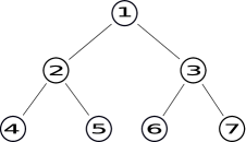
Figure 1: A height 3 binary tree $T_{2}^{3}$ with nodes numbered heap style.

It is not hard to show that a deterministic logspace-bounded polytime auxiliary pushdown automaton decides $BT_{d}(h,k)$, where $d$,$h$ and $k$ are input parameters. This implies by [Sud78] that $BT_{d}(h,k)$ belongs to the class $\mathbf{LogDCFL}$ of languages logspace reducible to a deterministic context-free language. The latter class lies between $\mathbf{L}$ and $\mathbf{LogCFL}$, but its relationship with $\mathbf{NL}$ is unknown (see [Mah07] for a recent survey). We conjecture that $BT_{d}(h,k)$ does not lie in $\mathbf{NL}$. A proof would separate $\mathbf{NL}$ and $\mathbf{LogCFL}$, and hence (by (1)) separate $\mathbf{NC}^{1}$ and $\mathbf{NC}^{2}$.

Thus we are interested in proving superlogarithmic space upper and lower bounds (for fixed degree $d\geq 2$) for $BT_{d}(h,k)$ and $FT_{d}(h,k)$. Notice that for each constant $k=k_{0}\geq 2$, $BT_{d}(h,k_{0})$ is an easy generalization of the Boolean formula value problem for balanced formulas, and hence it is in $\mathbf{NC}^{1}$ and $\mathbf{L}$. Thus it is important that $k$ be an unbounded input parameter.

We use branching programs (BPs) as a nonuniform model of Turing machine space: A lower bound of $s(n)$ on the number of BP states implies a lower bound of $\Theta(\log s(n))$ on Turing machine space, but to prove the converse we would need to supply the machine with an advice string for each input length. Thus BP state lower bounds are stronger than TM space lower bounds, but we do not know how to take advantage of the uniformity of TMs to get the supposedly easier lower bounds on TM space. In this paper all of our lower bounds are nonuniform and all of our upper bounds are uniform.

In the context of branching programs we think of $d$ and $h$ as fixed, and we are interested in how the number of states required grows with $k$. To indicate this point of view we write the function problem $FT_{d}(h,k)$ as $FT_{d}^{h}(k)$ and the Boolean problem $BT_{d}(h,k)$ as $BT_{d}^{h}(k)$. For this it turns out that $k$-way BPs are a convenient model, since an input for $BT_{d}^{h}(k)$ or $FT_{d}^{h}(k)$ is naturally presented as a tuple of elements in $[k]$. Each nonfinal state in a $k$-way BP queries a specific element of the tuple, and branches $k$ possible ways according to the $k$ possible answers.

It is natural to assume that the inputs to Turing machines are binary strings, so 2-way BPs are a closer model of TM space than are $k$-way BPs for $k>2$. But every 2-way BP is easily converted to a $k$-way BP with the same number of states, and every $k$-way BP can be converted to a 2-way BP with an increase of only a factor of $k$ in the number of states, so for the purpose of separating $\mathbf{L}$ and $\mathbf{P}$ we may as well use $k$-way BPs.

Of course the number of states required by a $k$-way BP to solve the Boolean problem $BT_{d}^{h}(k)$ is at most the number required to solve the function problem $FT_{d}^{h}(k)$. In the other direction it is easy to see (Lemma 3) that $FT_{d}^{h}(k)$ requires at most a factor of $k$ more states than $BT_{d}^{h}(k)$. From the point of view of separating $\mathbf{L}$ and $\mathbf{P}$ a factor of $k$ is not important. Nevertheless it is interesting to compare the two numbers, and in some cases (Corollary 25) we can prove tight bounds for both: For deterministic BPs solving height 3 trees they differ by a factor of $\log k$ rather than $k$.

The best (i.e. fewest states) algorithms that we know for deterministic $k$-way BPs solving $FT_{d}^{h}(k)$ come from black pebbling algorithms for trees: If $p$ pebbles suffice to pebble the tree $T^{h}_{d}$ then $O(k^{p})$ states suffice for a BP to solve $FT_{d}^{h}(k)$ (Theorem 10). This upper bound on states is tight (up to a constant factor) for trees of height $h=2$ or $h=3$ (Corollary 25), and we suspect that it may be tight for trees of any height.

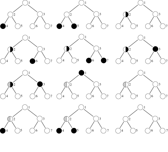
Figure 2: An optimal fractional pebbling sequence for the height 3 tree using 2.5 pebbles, all configurations included. The grey half circle means the white value of that node is $.5$, whereas unshaded area means absence of pebble value. So for example in the seventh configuration, node 2 has black value .5 and white value .5, node 3 has black value 1, and the remaining nodes all have black and white value 0.

There is a well-known generalization of black pebbling called black-white pebbling which naturally simulates nondeterministic algorithms. Indeed if $p$ pebbles suffice to black-white pebble $T^{h}_{d}$ then $O(k^{p})$ states suffice for a nondeterministic BP to solve $BT_{d}^{h}(k)$. However the best lower bound we can obtain for nondeterministic BPs solving $BT_{2}^{3}(k)$ (see Figure 1) is $\Omega(n^{2.5})$, whereas it takes 3 pebbles to black-white pebble the tree $T^{3}_{2}$. This led us to rethink the upper bound, and we discovered that there is indeed a nondeterministic BP with $O(k^{2.5})$ states which solves $BT_{2}^{3}(k)$. The algorithm comes from a black-white pebbling of $T^{3}_{2}$ using only 2.5 pebbles: It places a half-black pebble on node 2, a black pebble on node 3, and adds a half white pebble on node 2, allowing the root to be black-pebbled (see Figure 2 on page 2).

This led us to the idea of fractional pebbling in general, a natural generalization of black-white pebbling. A fractional pebble configuration on a tree assigns two nonnegative real numbers $b(i)$ and $w(i)$ totalling at most 1, to each node $i$ in the tree, with appropriate rules for removing and adding pebbles. The idea is to minimize the maximum total pebble weight on the tree during a pebbling procedure which starts and ends with no pebbles and has a black pebble on the root at some point.

It turns out that nondeterministic BPs nicely implement fractional pebbling procedures: If $p$ pebbles suffice to fractionally pebble $T^{h}_{d}$ then $O(k^{p})$ states suffice for a nondeterministic BP to solve $BT_{d}^{h}(k)$. After much work we have not been able to improve upon this $O(k^{p})$ upper bound for any $d,h\geq 2$. We prove it is optimal for trees of height 3 (Corollary 25).

We can prove that for fixed degree $d$ the number of pebbles required to pebble (in any sense) the tree $T^{h}_{d}$ grows as $\Theta(h)$, so the $p$ in the above best-known upper bounds of $O(k^{p})$ states grows as $\Theta(h)$. This and the following fact motivate further study of the complexity of $FT_{d}^{h}(k)$.

Fact 1

A lower bound of $\Omega(k^{r(h)})$ for any unbounded function $r(h)$ on the number of states required to solve $FT_{d}^{h}(k)$ implies that $\mathbf{L}\neq\mathbf{LogCFL}$ (Theorem 7 and Corollary 9).

Proving tight bounds on the number of pebbles required to fractionally pebble a tree turns out to be much more difficult than for the case of whole black-white pebbling. However we can prove good upper and lower bounds. For binary trees of any height $h$ we prove an upper bound of $h/2+1$ and a lower bound of $h/2-1$ (the upper bound is optimal for $h\leq 4$). These bounds can be generalized to $d$-ary trees (Theorem 15).

We introduce a natural semantic restriction on BPs which solve $BT_{d}^{h}(k)$ or $FT_{d}^{h}(k)$: A $k$-way BP is thrifty if it only queries the function $f(x_{1},\ldots,x_{d})$ associated with a node when $(x_{1},\ldots,x_{d})$ are the correct values of the children of the node.

It is not hard to see that the deterministic BP algorithms that implement black pebbling are thrifty. With some effort we were able to prove a converse (for binary trees): If $p$ is the minimum number of pebbles required to black-pebble $T^{h}_{2}$ then every deterministic thrifty BP solving $BT^{h}_{2}(k)$ (or $FT^{h}_{2}(k)$) requires $\Omega(k^{p})$ states. Thus any deterministic BP solving these problems with fewer states must query internal nodes $f_{i}(x,y)$ where $(x,y)$ are not the values of the children of node $i$. For the decision problem $BT^{h}_{2}(k)$ there is indeed a nonthrifty deterministic BP improving on the bound by a factor of $\log k$ (Theorem 24 (15)), and this is tight for $h=3$ (Corollary 25). But we have not been able to improve on thrifty BPs for solving any function problem $FT_{d}^{h}(k)$.

The nondeterministic BPs that implement fractional pebbling are indeed thrifty. However here the converse is far from clear: there is nothing in the definition of thrifty that hints at fractional pebbling. We have been able to prove that thrifty BPs cannot beat fractional pebbling for binary trees of height $h=4$ or less, but for general trees this is open.

It is not hard to see that for black pebbling, fractional pebbles do not help. This may explain why we have been able to prove tight bounds for deterministic thrifty BPs for all binary trees, but only for trees of height 4 or less for nondeterministic thrifty BPs.

We pose the following as another interesting open question:

Thrifty Hypothesis: Thrifty BPs are optimal among $k$-way BPs solving $FT_{d}^{h}(k)$.

Proving this for deterministic BPs would show $\mathbf{L}\neq\mathbf{LogDCFL}$, and for nondeterministic BPs would show $\mathbf{NL}\neq\mathbf{LogCFL}$. Disproving this would provide interesting new space-efficient algorithms and might point the way to new approaches for proving lower bounds.

The lower bounds mentioned above for unrestricted branching programs when the tree heights are small are obtained in two ways: First using the Nec̆iporuk method [Nec̆66], and second using a method that analyzes the state sequences of the BP computations. Using the state sequence method we have not yet beat the $\Omega(n^{2})$ deterministic branching program size barrier (neglecting log factors) inherent to the Nec̆iporuk method for Boolean problems, but we can prove lower bounds for function problems which cannot be matched by the Nec̆iporuk method (Theorems 27, 28, 31, 32). For nondeterministic branching programs with states of unbounded outdegree, we show that both methods yield a lower bound of $\Omega(n^{3/2})$ states (neglecting logs) for the decision problem $BT_{2}^{3}$, and this improves on the former $\Omega(n^{3/2})$ bound obtained for the number of edges [Pud87, Raz91] in such BPs.

1.1 Summary of Contributions

• We introduce a family of computation problems $FT_{d}^{h}(k)$ and $BT_{d}^{h}(k)$, $d,h\geq 2$, which we propose as good candidates for separating $\mathbf{L}$ and $\mathbf{NL}$ from apparently larger complexity classes in (1). Our goal is to prove space lower bounds for these problems by proving state lower bounds for $k$-way branching programs which solve them. For $h=3$ we can prove tight bounds for each $d\geq 2$ on the number of states required by $k$-way BPs to solve them, namely (from Corollary 25)

  $$\Theta(k^{(3/2)d-1/2})\mbox{ for nondeterministic BPs solving $BT^{3}_{d}(k)$}$$

  $$\Theta(k^{2d-1}/\log k)\mbox{ for deterministic BPs solving $BT^{3}_{d}(k)$}$$

  $$\Theta(k^{2d-1})\mbox{ for deterministic BPs solving $FT^{3}_{d}(k)$}$$

• We introduce a simple and natural restriction called thrifty on BPs solving $FT_{d}^{h}(k)$ and $BT_{d}^{h}(k)$. The best known upper bounds for deterministic BPs solving $FT_{d}^{h}(k)$ and for nondeterministic BPs solving $BT_{d}^{h}(k)$ are realized by thrifty BPs. Proving even much weaker lower bounds than these upper bounds for unrestricted BPs would separate $\mathbf{L}$ from $\mathbf{LogCFL}$ (see Fact 1 above). We prove that for binary trees deterministic thrifty BPs cannot do better than implement black pebbling (this is far from obvious).

• We formulate the Thrifty Hypothesis (see above). Either a proof or a disproof would have interesting consequences.

• We introduce fractional pebbling as a natural generalization of black-white pebbling for simulating nondeterministic space bounded computations. We prove almost tight lower bounds for fractionally pebbling binary trees (Theorem 15). The best known upper bounds for nondeterministic BPs solving $FT_{d}^{h}(k)$ come from fractional pebbling, and these can be implemented by thrifty BPs. An interesting open question is to prove that nondeterministic thrifty BPs cannot do better than implement fractional pebbling. (We prove this for $h=2,3,4$.)

• We use a “state sequence” method for proving size lower bounds for branching programs solving $FT_{d}^{h}(k)$ and $BT_{d}^{h}(k)$, and show that it improves on the Nec̆iporuk method for certain function problems.

The next major step is to prove good lower bounds for trees of height $h=4$. If we can prove the above Thrifty Hypothesis for deterministic BPs solving the function problem (and hence the decision problem) for trees of height 4, then we would beat the $\Omega(n^{2})$ limitation mentioned above on Nec̆iporuk’s method. See Section 6 (Conclusion) for this argument, and a comment about the nondeterministic case.

1.2 Relation to previous work

Taitslin [Tai05] proposed a problem similar to $BT_{2}^{h}(k)$ in which the functions attached to internal nodes are specific quasi groups, in an unsuccessful attempt to prove $\mathbf{NL}\neq\mathbf{P}$.

Gal, Koucky and McKenzie [GKM08] proved exponential lower bounds on the size of restricted $n$-way branching programs solving versions of the problem GEN. Like our problems $BT_{d}^{h}(k)$ and $FT_{d}^{h}(k)$, the best known upper bounds for solving GEN come from pebbling algorithms.

As a concrete approach to separating $\mathbf{NC}^{1}$ from $\mathbf{NC}^{2}$, Karchmer, Raz and Wigderson [KRW95] suggested proving that the circuit depth required to compose a Boolean function with itself $h$ times grows appreciably with $h$. They proposed the universal composition relation conjecture, stating that an abstraction of the composition problem requires high communication complexity, as an intermediate goal to validate their approach. This conjecture was later proved in two ways, first [EIRS01] using innovative information-theoretic machinery and then [HW93] using a clever new complexity measure that generalizes the subadditivity property implicit in Nec̆iporuk’s lower bound method [Nec̆66]. Proving the conjecture thus cleared the road for the approach, yet no sufficiently strong unrestricted circuit lower bounds could be proved using it so far.

Edmonds, Impagliazzo, Rudich and Sgall [EIRS01] noted that the approach would in fact separate $\mathbf{NC}^{1}$ from $\mathbf{AC}^{1}$. They also coined the name Iterated Multiplexor for the most general computational problem considered in [KRW95], namely composing in a tree-like fashion a set of explicitly presented Boolean functions, one per tree node. Our problem $FT_{d}^{h}(k)$ can be considered as a generalization of the Iterated Multiplexor problem in which the functions map $[k]^{d}$ to $[k]$ instead of $\{0,1\}^{d}$ to $\{0,1\}$. This generalization allows us to focus on getting lower bounds as a function of $k$ when the tree is fixed.

For time-restricted branching programs, Borodin, Razborov and Smolensky [BRS93] exhibited a family of Boolean functions that require exponential size to be computed by nondeterministic syntactic read-$k$ times BPs. Later Beame, Saks, Sun, and Vee [BSSV03] exhibited such functions that require exponential size to be computed by randomized BPs whose computation time is limited to $o(n\sqrt{\log n/\log\log n})$, where $n$ is the input length. However all these functions can be computed by polynomial size BPs when time is unrestricted.

In the present paper we consider branching programs with no time restriction such as read-$k$ times. However the smallest size deterministic BPs known to us that solve $FT_{d}^{h}(k)$ implement the black pebbling algorithm, and these BPs happen to be (syntactic) read-once.

1.3 Organization

The paper is organized as follows. Section 2 defines the main notions used in this paper, including branching programs and pebbling. Section 3 relates pebbling and branching programs to Turing machine space, noting in particular that a $k$-way BP size lower bound of $\Omega(k^{\mbox{\scriptsize function}(h)})$ for $BT_{d}^{h}(k)$ would show $\mathbf{L}\neq\mathbf{LogCFL}$. Section 4 proves upper and lower bounds on the number of pebbles required to black, black-white and fractionally pebble the tree $T^{h}_{d}$. These pebbling bounds are exploited in Section 5 to prove upper bounds on the size of branching programs. BP lower bounds are obtained using the Nec̆iporuk method in Subsection 5.1. Alternative proofs to some of these lower bounds using the “state sequence method” are given in Subsection 5.2. An example of a function problem for which the state sequence method beats the Nec̆iporuk method is given in Theorems 27 and 31. Subsection 5.3 contains bounds for thrifty branching programs.

2 Preliminaries

We assume some familiarity with complexity theory, such as can be found in [Gol08]. We write $[k]$ for $\{1,2,\ldots,k\}$. For $d,h\geq 2$ we use $T_{d}^{h}$ to denote the balanced $d$-ary tree of height $h$.

Warning: Here the height of a tree is the number of levels in the tree, as opposed to the distance from root to leaf. Thus $T^{2}_{2}$ has just 3 nodes.

We number the nodes of $T_{d}^{h}$ as suggested by the heap data structure. Thus the root is node 1, and in general the children of node $i$ are (when $d=2$) nodes $2i,2i+1$ (see Figure 1).

Definition 1 (Tree evaluation problems)

Given: The tree $T_{d}^{h}$ with each non-leaf node $i$ independently labeled with a function $f_{i}:[k]^{d}\rightarrow[k]$ and each leaf node independently labeled with an element from $[k]$, where $d,h,k\geq 2$.

Function evaluation problem $FT_{d}^{h}(k)$: Compute the value $v_{1}\in[k]$ of the root $1$ of $T_{d}^{h}$, where in general $v_{i}=a$ if $i$ is a leaf labeled $a$ and $v_{i}=f_{i}(v_{j_{1}},\ldots,v_{j_{d}})$ if the children of $i$ are $j_{1},\ldots,j_{d}$.

Boolean problem $BT_{d}^{h}(k)$: Decide whether $v_{1}=1$.

2.1 Branching programs

A family of branching programs serves as a nonuniform model of of a Turing machine. For each input size $n$ there is a BP $B_{n}$ in the family which models the machine on inputs of size $n$. The states (or nodes) of $B_{n}$ correspond to the possible configurations of the machine for inputs of size $n$. Thus if the machine computes in space $s(n)$ then $B_{n}$ has $2^{O(s(n))}$ states.

Many variants of the branching program model have been studied (see in particular the survey by Razborov [Raz91] and the book by Ingo Wegener [Weg00]). Our definition below is inspired by Wegener [Weg00, p. 239], by the $k$-way branching program of Borodin and Cook [BC82] and by its nondeterministic variant [BRS93, GKM08]. We depart from the latter however in two ways: nondeterministic branching program labels are attached to states rather than edges (because we think of branching program states as Turing machine configurations) and cycles in branching programs are allowed (because our lower bounds apply to this more powerful model).

Definition 2 (Branching programs)

A nondeterministic $k$-way branching program $B$ computing a total function $g:[k]^{m}\rightarrow R$, where $R$ is a finite set, is a directed rooted multi-graph whose nodes are called states. Every edge has a label from $[k]$. Every state has a label from $[m]$, except $|R|$ final sink states consecutively labelled with the elements from $R$. An input $(x_{1},\ldots,x_{m})\in[k]^{m}$ activates, for each $1\leq j\leq m$, every edge labelled $x_{j}$ out of every state labelled $j$. A computation on input $\vec{x}=(x_{1},\ldots,x_{m})\in[k]^{m}$ is a directed path consisting of edges activated by $\vec{x}$ which begins with the unique start state (the root), and either it is infinite, or it ends in the final state labelled $g(x_{1},\ldots,x_{m})$, or it ends in a nonfinal state labelled $j$ with no outedge labelled $x_{j}$ (in which case we say the computation aborts). At least one such computation must end in a final state. The size of $B$ is its number of states. $B$ is deterministic $k$-way if every non-final state has precisely $k$ outedges labelled $1,\ldots,k$. $B$ is binary if $k=2$.

We say that $B$ solves a decision problem (relation) if it computes the characteristic function of the relation.

A $k$-way branching program computing the function $FT_{d}^{h}(k)$ requires $k^{d}$ $k$-ary arguments for each internal node $i$ of $T^{h}_{d}$ in order to specify the function $f_{i}$, together with one $k$-ary argument for each leaf. Thus in the notation of Definition 1, $FT_{d}^{h}(k)$$:[k]^{m}\rightarrow R$ where $R=[k]$ and $m=\frac{d^{h-1}-1}{d-1}\cdot k^{d}+d^{h-1}$. Also $BT_{d}^{h}(k)$$:[k]^{m}\rightarrow\{0,1\}$.

For fixed $d,h$ we are interested in how the number of states required for a $k$-way branching program to compute $FT_{d}^{h}(k)$ and $BT_{d}^{h}(k)$ grows with $k$. We define $\mathsf{\#detFstates}^{h}_{d}(k)$ (resp. $\mathsf{\#ndetFstates}^{h}_{d}(k)$) to be the minimum number of states required for a deterministic (resp. nondeterministic) $k$-way branching program to solve $FT_{d}^{h}(k)$. Similarly we define $\mathsf{\#detBstates}^{h}_{d}(k)$ and $\mathsf{\#ndetBstates}^{h}_{d}(k)$ to be the number of states for solving $BT_{d}^{h}(k)$.

The next lemma shows that the function problem is not much harder to solve than the Boolean problem.

Lemma 3

$$\mathsf{\#detBstates}^{h}_{d}(k)\leq\mathsf{\#detFstates}^{h}_{d}(k)\leq k\cdot\mathsf{\#detBstates}^{h}_{d}(k)$$

$$\mathsf{\#ndetBstates}^{h}_{d}(k)\leq\mathsf{\#ndetFstates}^{h}_{d}(k)\leq k\cdot\mathsf{\#ndetBstates}^{h}_{d}(k)$$

Proof:    The left inequalities are obvious. For the others, we can construct a branching program solving the function problem from a sequence of $k$ programs solving Boolean problems, where the $i$th program determines whether the value of the root node is $i$. $\blacksquare$

Next we introduce thrifty programs, a restricted form of $k$-way branching programs for solving tree evaluation problems. Thrifty programs efficiently simulate pebbling algorithms, and implement the best known upper bounds for $\mathsf{\#ndetBstates}^{h}_{d}(k)$ and $\mathsf{\#detFstates}^{h}_{d}(k)$, and are within a factor of $\log k$ of the best known upper bounds for $\mathsf{\#detBstates}^{h}_{d}(k)$. In Section 5 we prove tight lower bounds for deterministic thrifty programs which solve $BT_{d}^{h}(k)$ and $FT_{d}^{h}(k)$.

Definition 4 (Thrifty branching program)

A deterministic $k$-way branching program which solves $FT_{d}^{h}(k)$ or $BT_{d}^{h}(k)$ is thrifty if during the computation on any input every query $f_{i}(\vec{x})$ to an internal node $i$ of $T^{h}_{d}$ satisfies the condition that $\vec{x}$ is the tuple of correct values for the children of node $i$. A nondeterministic such program is thrifty if for every input every computation which ends in a final state satisfies the above restriction on queries.

Note that the restriction in the above definition is semantic, rather than syntactic. It somewhat resembles the semantic restriction used to define incremental branching programs in [GKM08]. However we are able to prove strong lower bounds using our semantic restriction, but in [GKM08] a syntactic restriction was needed to prove lower bounds.

2.2 One function is enough

The theorem in this section is not used in the sequel.

It turns out that the complexities of $FT_{d}^{h}(k)$ and $BT_{d}^{h}(k)$ are not much different if we require all functions assigned to internal nodes to be the same. To denote this restricted version of the problems we replace $F$ by $\hat{F}$ and $B$ by $\hat{B}$. Thus $\hat{F}T_{d}^{h}(k)$ is the function problem for $T^{h}_{d}$ when all node functions are the same, and $\hat{B}T_{d}^{h}(k)$ is the corresponding Boolean problem. To specify an instance of one of these new problems we need only give one copy of the table for the common node function $\hat{f}$, together with the values for the leaves.

Theorem 5

Let $N=(d^{h}-1)/(d-1)$ be the number of nodes in the tree $T^{h}_{d}$. Any $Nk$-way branching program $\hat{B}$ solving $\hat{F}T_{d}^{h}(Nk)$ (resp. $\hat{B}T_{d}^{h}(Nk)$) can be transformed to a $k$-way branching program $B$ solving $FT_{d}^{h}(k)$ (resp. $BT_{d}^{h}(k)$), where $B$ has no more states than $\hat{B}$ and $B$ is deterministic iff $\hat{B}$ is deterministic. Also for each $d\geq 2$ the decision problem $BT_{d}(h,k)$ is log space reducible to $\hat{B}T_{d}(h,k)$ (where $h,k$ are input parameters).

Proof:    Given an instance $I$ of $FT_{d}^{h}(k)$ (or $BT_{d}^{h}(k)$) we can find a corresponding instance $\hat{I}$ of $\hat{F}T_{d}^{h}(Nk)$ (or $\hat{B}T_{d}^{h}(Nk)$) by coding the set of all functions $f_{i}$ associated with internal nodes $i$ in $I$ by a single function $\hat{f}$ associated with each node of $\hat{I}$. Here we represent each element of $[Nk]$ by a pair $\langle i,x\rangle$, where $i\in[N]$ represents a node in $T^{h}_{d}$ and $x\in[k]$. We want to satisfy the following Claim:

Claim: If a node $i$ has a value $x$ in $I$ then node $i$ has value $\langle i,x\rangle$ in $\hat{I}$.

Thus if $i$ is a leaf node, then we define the leaf value for node $i$ in $\hat{I}$ to be $\langle i,x\rangle$, where $x$ is the value of leaf $i$ in $I$.

We define the common internal node function $\hat{f}$ as follows. If nodes $i_{1},\ldots,i_{d}$ are the children of node $j$ in $T^{h}_{d}$, then

$$\hat{f}(\langle i_{1},x_{1}\rangle,\ldots,\langle i_{d},x_{d}\rangle)=\langle j,f_{j}(x_{1},\ldots,x_{d})\rangle$$ (2)

The value of $\hat{f}$ is irrelevant (make it $\langle 1,1\rangle$) if nodes $i_{1},\ldots,i_{d}$ are not the children of $j$.

An easy induction on the height of a node $i$ shows that the above Claim is satisfied.

Note that the value $x$ of the root node $1$ in $I$ is easily determined by the value $\langle 1,x\rangle$ of the root in $\hat{I}$. We specify that the pair $\langle 1,1\rangle$ has value 1 in $[N]$, so $I$ is a YES instance of the decision problem $BT_{d}^{h}(k)$ iff $\hat{I}$ is a YES instance of $\hat{B}T_{d}^{h}(Nk)$.

To complete the proof of the last sentence in the theorem we note that the number of bits needed to specify $I$ is $\Theta(Nk^{d}\log k)$, and the number of bits to specify $\hat{I}$ is dominated by the number to specify $\hat{f}$, which is $O((Nk)^{d}\log(Nk))$. Thus the transformation from $I$ to $\hat{I}$ is length-bounded by a polynomial in length of its argument, and it is not hard to see that it can be carried out in log space.

Now we prove the first part of the theorem. Given an $Nk$-way BP $\hat{B}$ solving $\hat{B}T_{d}^{h}(Nk)$ (resp. $\hat{F}T_{d}^{h}(Nk)$) we can find a corresponding $k$-way BP $B$ solving $BT_{d}^{h}(k)$ (resp. $FT_{d}^{h}(k)$) as follows.

The idea is that on input instance $I$, $B$ acts like $\hat{B}$ on input $\hat{I}$. Thus for each state $\hat{q}$ in $\hat{B}$ that queries a leaf node $i$, the corresponding state $q$ in $B$ queries $i$, and for each possible answer $x\in[k]$, $B$ has an outedge labelled $x$ corresponding to the edge from $\hat{q}$ labelled $\langle i,x\rangle$. If $\hat{q}$ queries $\hat{f}$ at arguments as in (2) (where $i_{1},\ldots,i_{d}$ are the children of node $j$) then $q$ queries $f_{j}(x_{1},\ldots,x_{d})$ and for each $x\in[k]$, $q$ has an outedge labelled $x$ corresponding to the edge from $\hat{q}$ labelled $\langle j,x\rangle$. If $i_{1},\ldots,i_{d}$ are not the children of $j$, then the node $q$ is not necessary in $B$, since the answer to the query is always the default $\langle 1,1\rangle$.

In case $\hat{B}$ is solving the function problem $\hat{F}T_{d}^{h}(Nk)$ then each output state labelled $\langle 1,x\rangle$ is relabelled $x$ in $B$ (recall that the root of $T^{h}_{d}$ is number 1). Any output state $q$ labelled $\langle i,x\rangle$ where $i>1$ will never be reached in $B$ (since the value of the root node of $\hat{I}$ always has the form $\langle 1,x\rangle$) so $q$ can be deleted. For any edge in $\hat{B}$ leading to $q$ the corresponding edge in $B$ can lead anywhere. $\blacksquare$

One goal of this paper is to motivate trying to show $BT_{d}(h,k)\notin\mathbf{L}$. By Theorem 5 this is equivalent to showing $\hat{B}T_{d}(h,k)\notin\mathbf{L}$. Further our suggested method is to try proving for each fixed $h$ a lower bound of $\Omega(k^{r(h})$ on the number of states required for a $k$-way BP to solve $FT_{d}^{h}(k)$, where $r(h)$ is any unbounded function (see Corollary 9 below). Again acording to Theorem 5 (since $N$ is a constant) technically speaking we may as well assume that all the node functions in the instance of $FT_{d}^{h}(k)$ are the same. However in practice this assumption is not helpful in proving a lower bound. For example Theorem 32 states that $k^{3}$ states are required for a deterministic $k$-way BP to solve $FT^{3}_{2}(k)$, and the proof assigns three different functions to the three internal nodes of the binary tree of height 3.

2.3 Pebbling

The pebbling game for dags was defined by Paterson and Hewitt [PH70] and was used as an abstraction for deterministic Turing machine space in [Coo74]. Black-white pebbling was introduced in [CS76] as an abstraction of nondeterministic Turing machine space (see [Nor09] for a recent survey).

Here we define and use three versions of the pebbling game. The first is a simple ‘black pebbling’ game: A black pebble can be placed on any leaf node, and in general if all children of a node $i$ have pebbles, then one of the pebbles on the children can be slid to $i$ (this is a “black sliding move’)’. Any black pebble can be removed at any time. The goal is to pebble the root, using as few pebbles as possible. The second version is ‘whole’ black-white pebbling as defined in [CS76] with the restriction that we do not allow “white sliding moves”. Thus if node $i$ has a white pebble and each child of $i$ has a pebble (either black or white) then the white pebble can be removed. (A white sliding move would apply if one of the children had no pebble, and the white pebble on $i$ was slid to the empty child. We do not allow this.) A white pebble can be placed on any node at any time. The goal is to start and end with no pebbles, but to have a black pebble on the root at some time.

The third is a new game called fractional pebbling, which generalizes whole black-white pebbling by allowing the black and white pebble value of a node to be any real number between 0 and 1. However the total pebble value of each child of a node $i$ must be 1 before the black value of $i$ is increased or the white value of $i$ is decreased. Figure 2 illustrates two configurations in an optimal fractional pebbling of the binary tree of height three using 2.5 pebbles.

Our motivation for choosing these definitions is that we want pebbling algorithms for trees to closely correspond to $k$-way branching program algorithms for the tree evaluation problem.

We start by defining fractional pebbling, and then define the other two notions as restrictions on fractional pebbling.

Definition 6 (Pebbling)

A fractional pebble configuration on a rooted $d$-ary tree $T$ is an assignment of a pair of real numbers $(b(i),w(i))$ to each node $i$ of the tree, where

$$0\leq b(i),w(i)$$ (3)

$$b(i)+w(i)\leq 1$$ (4)

Here $b(i)$ and $w(i)$ are the black pebble value and the white pebble value, respectively, of $i$, and $b(i)+w(i)$ is the pebble value of $i$. The number of pebbles in the configuration is the sum over all nodes $i$ of the pebble value of $i$. The legal pebble moves are as follows (always subject to maintaining the constraints (3), (4)): (i) For any node $i$, decrease $b(i)$ arbitrarily, (ii) For any node $i$, increase $w(i)$ arbitrarily, (iii) For every node $i$, if each child of $i$ has pebble value 1, then decrease $w(i)$ to 0, increase $b(i)$ arbitrarily, and simultaneously decrease the black pebble values of the children of $i$ arbitrarily.

A fractional pebbling of $T$ using $p$ pebbles is any sequence of (fractional) pebbling moves on nodes of $T$ which starts and ends with every node having pebble value 0, and at some point the root has black pebble value 1, and no configuration has more than $p$ pebbles.

A whole black-white pebbling of $T$ is a fractional pebbling of $T$ such that $b(i)$ and $w(i)$ take values in $\{0,1\}$ for every node $i$ and every configuration. A black pebbling is a black-white pebbling in which $w(i)$ is always 0.

Notice that rule (iii) does not quite treat black and white pebbles dually, since the pebble values of the children must each be 1 before any decrease of $w(i)$ is allowed. A true dual move would allow increasing the white pebble values of the children so they all have pebble value 1 while simultaneously decreasing $w(i)$. In other words, we allow black sliding moves, but disallow white sliding moves. The reason for this (as mentioned above) is that nondeterministic branching programs can simulate the former, but not the latter.

We use $\mathsf{\#pebbles}(T)$, $\mathsf{\#BWpebbles}(T)$, and $\mathsf{\#FRpebbles}(T)$ respectively to denote the minimum number of pebbles required to black pebble $T$, black-white pebble $T$, and fractional pebble $T$. Bounds for these values are given in Section 4. For example for $d=2$ we have $\mathsf{\#pebbles}(T^{h}_{2})=h$, $\mathsf{\#BWpebbles}(T^{h}_{2})=\lceil h/2\rceil+1$, and $\mathsf{\#FRpebbles}(T^{h}_{2})\leq h/2+1$. In particular $\mathsf{\#FRpebbles}(T^{3}_{2})=2.5$ (see Figure 2).

3 Connecting TMs, BPs, and Pebbling

Let $FT_{d}(h,k)$ be the same as $FT_{d}^{h}(k)$ except now the inputs vary with both $h$ and $k$, and we assume the input to $FT_{d}(h,k)$ is a binary string $X$ which codes $h$ and $k$ and codes each node function $f_{i}$ for the tree $T^{h}_{d}$ by a sequence of $k^{d}$ binary numbers and each leaf value by a binary number in $[k]$, so $X$ has length

$$|X|=\Theta(d^{h}k^{d}\log k)$$ (5)

The output is a binary number in $[k]$ giving the value of the root.

The problem $BT_{d}(h,k)$ is the Boolean version of $FT_{d}(h,k)$: The input is the same, and the instance is true iff the value of the root is 1.

Obviously $BT_{d}(h,k)$ and $FT_{d}(h,k)$ can be solved in polynomial time, but we can prove a stronger result.

Theorem 7

The problem $BT_{d}(h,k)$ is in $\mathbf{LogDCFL}$, even when $d$ is given as an input parameter.

Proof:    By [Sud78] if suffices to show that $BT_{d}(h,k)$ is solved by some deterministic auxiliary pushdown automaton $M$ in $\log$ space and polynomial time. The algorithm for $M$ is to use its stack to perform a depth-first search of the tree $T^{h}_{d}$, where for each node $i$ it keeps a partial list of the values of the children of $i$, until it obtains all $d$ values, at which point it computes the value of $i$ and pops its stack, adding that value to the list for the parent node.

Note that the length $n$ of an input instance is about $d^{k}k^{d}\log k$ bits, so $\log n>d\log k$, so $M$ has ample space on its work tape to write all $d$ values of the children of a node $i$. $\blacksquare$

The best known upper bounds on branching program size for $FT_{d}^{h}(k)$ grow as $k^{\Omega(h)}$. The next result shows (Corollary 9) that any lower bound with a nontrivial dependency on $h$ in the exponent of $k$ for deterministic (resp. nondeterministic) BP size would separate $\mathbf{L}$(resp. $\mathbf{NL}$) from $\mathbf{LogDCFL}$.

Theorem 8

For each $d\geq 2$, if $BT_{d}(h,k)$ is in $\mathbf{L}$ (resp. $\mathbf{NL}$) then there is a constant $c_{d}$ and a function $f_{d}(h)$ such that $\mathsf{\#detFstates}^{h}_{d}(k)\leq f_{d}(h)k^{c_{d}}$ (resp. $\mathsf{\#ndetFstates}^{h}_{d}(k)\leq f_{d}(h)k^{c_{d}}$) for all $h,k\geq 2$.

Proof:    By Lemma 3 it suffices to prove this for $\mathsf{\#detBstates}^{h}_{d}(k)$ and $\mathsf{\#ndetBstates}^{h}_{d}(k)$ instead of $\mathsf{\#detFstates}^{h}_{d}(k)$ and $\mathsf{\#ndetFstates}^{h}_{d}(k)$. In general a Turing machine which can enter at most $C$ different configurations on all inputs of a given length $n$ can be simulated (for inputs of length $n$) by a binary (and hence $k$-ary) branching program with $C$ states. Each Turing machine using space $O(\log n)$ has at most $n^{c}$ possible configurations on any input of length $n\geq 2$, for some constant $c$. By (5) the input for $BT_{d}(h,k)$ has length $n=\Theta(d^{h}k^{d}\log k)$, so there are at most $(d^{h}k^{d}\log k)^{c^{\prime}}$ possible configurations for a log space Turing machine solving $BT_{d}(h,k)$, for some constant $c^{\prime}$. So we can take $f_{d}(h)=d^{c^{\prime}h}$ and $c_{d}=c^{\prime}(d+1)$. $\blacksquare$

Corollary 9

Fix $d\geq 2$ and any unbounded function $r(h)$. If $\mathsf{\#detFstates}^{h}_{d}(k)\in\Omega(k^{r(h)})$ then $BT_{d}(h,k)\notin\mathbf{L}$. If $\mathsf{\#ndetFstates}^{h}_{d}(k)\in\Omega(k^{r(h)})$ then $BT_{d}(h,k)\notin\mathbf{NL}$.

The next result connects pebbling upper bounds with upper bounds for thrifty branching programs.

Theorem 10

(i) If $T^{h}_{d}$ can be black pebbled with $p$ pebbles, then deterministic thrifty branching programs with $O(k^{p})$ states can solve $FT_{d}^{h}(k)$ and $BT_{d}^{h}(k)$.

(ii) If $T^{h}_{d}$ can be fractionally pebbled with $p$ pebbles then nondeterministic thrifty branching programs can solve $BT_{d}^{h}(k)$ with $O(k^{p})$ states.

Proof:    Consider the sequence $C_{0},C_{1},\ldots C_{\tau}$ of pebble configurations for a black pebbling of $T^{h}_{d}$ using $p$ pebbles. We may as well assume that the root is pebbled in configuration $C_{\tau}$, since all pebbles could be removed in one more step at no extra cost in pebbles. We design a thrifty branching program $B$ for solving $FT_{d}^{h}(k)$ as follows. For each pebble configuration $C_{t}$, program $B$ has $k^{p}$ states; one state for each possible assignment of a value from $[k]$ to each of the $p$ pebbles. Hence $B$ has $O(k^{p})$ states, since $\tau$ is a constant independent of $k$. Consider an input $I$ to $FT_{d}^{h}(k)$, and let $v_{i}$ be the value in $[k]$ which $I$ assigns to node $i$ in $T^{h}_{d}$ (see Definition 1). We design $B$ so that on $I$ the computation of $B$ will be a state sequence $\alpha_{0},\alpha_{1},\ldots,\alpha_{\tau}$, where the state $\alpha_{t}$ assigns to each pebble the value $v_{i}$ of the node $i$ that it is on. (If a pebble is not on any node, then its value is 1.)

For the initial pebble configuration no pebbles have been assigned to nodes, so the initial state of $B$ assigns the value 1 to each pebble. In general if $B$ is in a state $\alpha$ corresponding to configuration $C_{t}$, and the next configuration $C_{t+1}$ places a pebble $j$ on node $i$, then the state $\alpha$ queries the node $i$ to determine $v_{i}$, and moves to a new state which assigns $v_{i}$ to the pebble $j$ and assigns 1 to any pebble which is removed from the tree. Note that if $i$ is an internal node, then all children of $i$ must be pebbled at $C_{t}$, so the state $\alpha$ ‘knows’ the values $v_{j_{1}},\ldots,v_{j_{d}}$ of the children of $i$, so $\alpha$ queries $f_{i}(v_{j_{1}},\ldots,v_{j_{d}})$.

When the computation of $B$ reaches a state $\alpha_{\tau}$ corresponding to $C_{\tau}$, then $\alpha_{\tau}$ determines the value of the root (since $C_{\tau}$ has a pebble on the root), so $B$ moves to a final state corresponding to the value of the root.

The argument for the case of whole black-white pebbling is similar, except now the value for each white pebble represents a guess for the value $v_{i}$ of the node it is on. If the pebbling algorithm places a white pebble $j$ on a node at some step, then the corresponding state of $B$ nondeterministically moves to any state in which the values of all pebbles except $j$ are the same as before, but the value of $j$ can be any value in $[k]$. If the pebbling algorithm removes a white pebble $j$ from a node $i$, then the corresponding state has a guess $v^{\prime}_{i}$ for the value of $i$, and either $i$ is a leaf, or all children of $i$ must be pebbled. The corresponding state of $B$ queries $i$ to determine its true value $v_{i}$. If $v_{i}\neq v^{\prime}_{i}$ then the computation aborts (i.e. all outedges from the state have label $v^{\prime}_{i}$). Otherwise $B$ assigns $j$ the value 1 and continues.

When $B$ reaches a state $\alpha$ corresponding to a pebble configuration $C_{t}$ for which the root has a black pebble $j$, then $\alpha$ knows whether or not the tentative value assigned to the root is 1. All future states remember whether the tentative value is 1. If the computation successfully (without aborting) reaches a state $\alpha_{\tau}$ corresponding to the final pebble configuration $C_{\tau}$, then $B$ moves to the final state corresponding to output 1 or output 0, depending on whether the tentative root value is 1.

Now we consider the case in which $C_{0},\ldots,C_{\tau}$ represents a fractional pebbling computation. If $b(i),w(i)$ are the black and white pebbled values of node $i$ in configuration $C_{t}$, then a state $\alpha$ of $B$ corresponding to $C_{t}$ will remember a fraction $b(i)+w(i)$ of the $\log k$ bits specifying the value $v_{i}$ of the node $i$, where the fraction $b(i)$ of bits are verified, and the fraction $w(i)$ of bits are conjectured. In general these numbers of bits are not integers, so they are rounded up to the next integer. This rounding introduces at most two extra bits for each node in $T^{h}_{d}$, for a total of at most $2T$ extra bits, where $T$ is the number of nodes in $T^{h}_{d}$. Since the sum over all nodes of all pebble values is at most $p$, the total number of bits that need to be remembered for a given pebble configuration is at most $p\log k+2T$, where $T$ is a constant. Associated with each step in the fractional pebbling there are $2^{p\log k+2T}=O(k^{p})$ states in the branching program, one for each setting of these bits. These bits can be updated for each of the three possible fractional pebbling moves (i), (ii), (iii) in Definition 6 in a manner similar to that for whole black-white pebbling.

It is easy to see that in all cases the branching programs described satisfy the thrifty requirement that an internal node is queried only at the correct values for its children (or, in the black-white and fractional cases, the program aborts if an incorrect query is made because of an incorrect guess for the value of a white-pebbled node). $\blacksquare$

Corollary 11

$\mathsf{\#detFstates}^{h}_{d}(k)=O(k^{\mathsf{\#pebbles}(T^{h}_{d})})$ and $\mathsf{\#ndetFstates}^{h}_{d}(k)=O(k^{\mathsf{\#FRpebbles}(T^{h}_{d})})$.

4 Pebbling Bounds

4.1 Previous results

We start by summarizing what is known about whole black and black-white pebbling numbers as defined at the end of Definition 6 (i.e. we allow black sliding moves but not white sliding moves).

The following are minor adaptations of results and techniques that have been known since work of Loui, Meyer auf der Heide and Lengauer-Tarjan [Lou79, adH79, LT80] in the late ’70s. They considered pebbling games where sliding moves were either disallowed or permitted for both black and white pebbles, in contrast to our results below.

We always assume $h\geq 2$ and $d\geq 2$.

Theorem 12

$\mathsf{\#pebbles}(T^{h}_{d})=(d-1)h-d+2$.

Proof:    For $h=2$ this gives $\mathsf{\#pebbles}(T^{2}_{d})=d$, which is obviously correct. In general we show $\mathsf{\#pebbles}(T^{h+1}_{d})=\mathsf{\#pebbles}(T^{h}_{d})+d-1$, from which the theorem follows.

The following pebbling strategy gives the upper bound: Let the root be node $1$ and the children be $2\ldots d+1$. Pebble the nodes $2\ldots d+1$ in order using the optimal number of pebbles for $T^{h-1}_{d}$, leaving a black pebble at each node. Note that for the black pebble game, the complexity of pebbling in the game where a pebble remains on the root is the same as for the game where the root has a black pebble on it at some point. The maximum number of pebbles at any point on the tree is $d-1+\mathsf{\#pebbles}(T^{h-1}_{d})$. Now slide the black pebble from node $1$ to the root, and then remove all pebbles.

For the lower bound, consider the time $t$ at which the children of the root all have black pebbles on them. There must be a final time $t^{\prime}$ before $t$ at which one of the sub-trees rooted at $2,3,\ldots d+1$ had $T^{h}_{d}$ pebbles on it. This is because pebbling any of these subtrees requires at least $T^{h}_{d}$ pebbles, by definition. At time $t^{\prime}$, all the other subtrees must have at least 1 black pebble each on them. If not, then there is a subtree $T$ which does not, and it would have to be pebbled before time $t$, which contradicts the definition of $t^{\prime}$. Thus at time $t^{\prime}$, there are at least $T^{h}_{d}+d-1$ pebbles on the tree. $\blacksquare$

Theorem 13

For $d=2$ and $d$ odd:

$$\mathsf{\#BWpebbles}(T^{h}_{d})=\lceil(d-1)h/2\rceil+1$$ (6)

For $d$ even:

$$\mathsf{\#BWpebbles}(T^{h}_{d})\leq\lceil(d-1)h/2\rceil+1$$ (7)

When $d$ is odd, this number is the same as when white sliding moves are allowed.

Proof:    We divide the proof into three parts.

Part I:
We show (6) when $d$ is odd.

For $h=2$ this gives $\mathsf{\#BWpebbles}(T^{2}_{d})=d$, which is obviously correct. In general for odd $d$ we show

$$\mathsf{\#BWpebbles}(T^{h+1}_{d})=\mathsf{\#BWpebbles}(T^{h}_{d})+(d-1)/2$$ (8)

from which the theorem follows for this case.

For the upper bound for the left hand side, we strengthen the induction hypothesis by asserting that during the pebbling there is a critical time at which the root has a black pebble and there are at most $\mathsf{\#BWpebbles}(T^{h}_{d})-(d-1)/2$ pebbles on the tree (counting the pebble on the root). This can be made true when $h=2$ by removing all the pebbles on the leaves after the root is pebbled.

To pebble the tree $T^{h+1}_{d}$, note that we are allowed $(d-1)/2$ extra pebbles over those required to pebble $T^{h}_{d}$. Start by placing black pebbles on the left-most $(d-1)/2$ children of the root, and removing all other pebbles. Now go through the procedure for pebbling the middle principal subtree, stopping at the critical time, so that there is a black pebble on the middle child of the root and at most $\mathsf{\#BWpebbles}(T^{h}_{d})-(d-1)/2$ pebbles on the middle subtree. Now place white pebbles on the remaining $(d-1)/2$ children of the root, slide a black pebble to the root, and remove all black pebbles on the children of the root. This is the critical time for pebbling $T^{h+1}_{d}$: note that there are at most $\mathsf{\#BWpebbles}(T^{h}_{d})$ pebbles on the tree (we removed the black pebble on the root of the middle subtree).

Now remove the pebble on the root and remove all pebbles on the middle subtree by completing its pebbling (keeping the $(d-1)/2$ white pebbles on the children in place). Finally remove the remaining $(d-1)/2$ white pebbles one by one, simply by pebbling each subtree, and removing the white pebble at the root of the subtree instead of black-pebbling it.

To prove the lower bound for the left hand side of (8), we strengthen the induction hypothesis so that now a black-white pebbling allows white sliding moves, and the root may be pebbled by either a black pebble or a white pebble. (Note that for the base case the tree $T^{2}_{d}$ still requires $d$ pebbles.) Consider such a pebbling of $T^{h+1}_{d}$ which uses as few moves as possible. Consider a time $t$ at which all children of the root have pebbles on them (i.e. just before the root is black pebbled or just after a white pebble on the root is removed). For each child $i$, let $t_{i}$ be a time at which the tree rooted at $i$ has $\mathsf{\#BWpebbles}(T^{h}_{d})$ pebbles on it. We may assume

$$t_{2}<t_{3}<\ldots<t_{d+1}$$

Let $m=(d+3)/2$ be the middle child. If $t_{m}<t$ then each of the $(d-1)/2$ subtrees rooted at $i$ for $i<m$ has at least one pebble on it at time $t_{m}$, since otherwise the effort made to place $\mathsf{\#BWpebbles}(T^{h}_{d})$ pebbles on it earlier is wasted. Hence (8) holds for this case. Similarly if $t_{m}>t$ then each of the $(d-1)/2$ subtrees rooted at $i$ for $i>m$ has at least one pebble on it at time $t_{m}$, since otherwise the effort to place $T^{h}_{d}$ pebbles on it later is wasted, so again (8) holds.

Part II:
We prove (7) for even degree $d$:

$$\mathsf{\#BWpebbles}(T^{h}_{d})\leq\lceil(d-1)h/2\rceil+1$$

For $h=2$ the formula gives $\mathsf{\#BWpebbles}(T^{2}_{d})=d$, which is obviously correct. For $h=3$ the formula gives $\mathsf{\#BWpebbles}(T^{3}_{d})=(3/2)d$, which can be realized by black-pebbling $d/2+1$ of the root’s children and white-pebbling the rest. In general it suffices to prove the following recurrence:

$$\mathsf{\#BWpebbles}(T^{h+2}_{d})\leq\mathsf{\#BWpebbles}(T^{h}_{d})+d-1$$ (9)

We strengthen the induction hypothesis by asserting that during the pebbling of $T^{h}_{d}$ there is a critical time at which the root has a black pebble and there are at most $\mathsf{\#BWpebbles}(T^{h}_{d})-(d-1)$ pebbles on the tree (counting the pebble on the root). This is easy to see when $h=2$ and $h=3$.

We prove the recurrence as follows. We want to pebble $T^{h+2}_{d}$ using $d-1$ more pebbles than is required to pebble $T^{h}_{d}$. Let us call the children of the root $c_{1},\ldots,c_{d}$. We start by placing black pebbles on $c_{1},\ldots c_{d/2}$. We illustrate how to do this by showing how to place a black pebble on $c_{d/2}$ after there are black pebbles on nodes $c_{1},\ldots c_{d/2-1}$. At this point we still have $d/2$ extra pebbles left among the original $d-1$. Let us assign the names $c^{\prime}_{1},\ldots c^{\prime}_{d}$ to the children of $c_{d/2}$. Use the $d/2$ extra pebbles to put black pebbles on $c^{\prime}_{1},\ldots,c^{\prime}_{d/2}$. Now run the procedure for pebbling the subtree rooted at $c^{\prime}_{d/2+1}$ up to the critical time, so there is a black pebble on $c^{\prime}_{d/2+1}$. Now place white pebbles on the remaining $d/2-1$ children of $c_{d/2}$, slide a black pebble up to $c_{d/2}$, remove the remaining black pebbles on the children of $c_{d/2}$, and complete the pebbling procedure for the subtree rooted at $c^{\prime}_{d/2+1}$, so that subtree has no pebbles. Now remove the white pebbles on the remaining $d/2-1$ children of $c_{d/2}$ using the remaining $d/2-1$ extra pebbles.

At this point there are black pebbles on nodes $c_{1},\ldots,c_{d/2}$, and no other pebbles on the tree. We now place a black pebble on $c_{d/2+1}$ as follows. Let us assign the names $c^{\prime\prime}_{1},\ldots c^{\prime\prime}_{d}$ to the children of $c_{d/2+1}$. Use the remaining $d/2-1$ extra pebbles to place black pebbles on $c^{\prime\prime}_{1},\ldots,c^{\prime\prime}_{d/2-1}$. Now run the pebble procedure on the subtree rooted at $c^{\prime\prime}_{d/2}$ up to the critical time, so $c^{\prime\prime}_{d/2}$ has a black pebble. Now place white pebbles on the remaining $d/2$ children of $c_{d/2+1}$, slide a black pebble up to $c_{d/2+1}$, remove the remaining black pebbles on the children of $c_{d/2+1}$, place white pebbles on the remaining $d/2-1$ children of the root, slide a black pebble up to the root, and remove the remaining black pebbles from the children of the root.

This is now the critical time for the procedure pebbling $T^{h+2}_{d}$. There is a black pebble on the root, $d/2-1$ white pebbles on the children of the root, $d/2$ white pebbles on the children of $c_{d/2+1}$, and at most $\mathsf{\#BWpebbles}(T^{h}_{d})-d$ pebbles on the subtree rooted at $c^{\prime\prime}_{d/2}$ (we’ve removed the black pebble on $c^{\prime\prime}_{d/2}$), making a total of at most $\mathsf{\#BWpebbles}(T^{h}_{d})$ pebbles on the tree.

Now remove the black pebble from the root and complete the pebble procedure for the subtree rooted at $c^{\prime\prime}_{d/2}$ to remove all pebbles from that subtree. There remain $d/2-1$ white pebbles on the children of the root and $d/2$ white pebbles on the children of $c_{d/2+1}$, making a total of $d-1$ white pebbles. Now remove each of the white pebbles on the children of $c_{d/2+1}$ by pebbling each of these subtrees in turn. Finally we can remove each of the remaining $d/2-1$ white pebbles on the children of the root by a process similar to the one used to place $d/2$ black pebbles on the children of the root at the beginning of the procedure (we now in effect have one more pebble to work with).

Part III:
Finally we give the lower bound for the case $d=2$:

$$\mathsf{\#BWpebbles}(T^{h}_{2})\geq\lceil h/2\rceil+1$$

Clearly 2 pebbles are required for the tree of height 2, and it is easy to show that 3 pebbles are required for the height 3 tree.

In general it suffices to show that the binary tree $T$ of height $h+2$ requires at least one more pebble than the binary tree of height $h$. Suppose otherwise, and consider a pebbling of $T$ that uses the minimum number of pebbles required for the tree of height $h$, and assume that the pebbling is as short as possible. Let $t_{1}$ be a time when the root has a black pebble. For $i=3,4,5$ there must be a time $t_{i}$ when all the pebbles are on the subtree rooted at node $i$. This is because node $i$ must be pebbled at some point, and if the pebble is white then right after the white pebble is removed we could have placed a black pebble in its place (since we do not allow white sliding moves).

Suppose that $\{t_{1},t_{3},t_{4},t_{5}\}$ are ordered such that

$$t_{i_{1}}<t_{i_{2}}<t_{i_{3}}<t_{i_{4}}$$

Then $t_{1}$ cannot be either $t_{i_{3}}$ or $t_{i_{4}}$ since otherwise at time $t_{i_{2}}$ there are no pebbles on the subtree rooted at node $i_{1}$ and hence its earlier pebbling was wasted (since the root has yet to be pebbled). Similarly if $t_{1}$ is either $t_{i_{1}}$ or $t_{i_{2}}$ then at time $t_{i_{3}}$ there are no pebbles on the subtree rooted at $i_{4}$, and since the root has already been pebbled the later pebbling of this subtree is wasted. $\blacksquare$

4.2 Results for fractional pebbling

The concept of fractional pebbling is new. Determining the minimum number $p$ of pebbles required to fractionally pebble $T^{h}_{d}$ is important since $O(k^{p})$ is the best known upper bound on the number of states required by a nondeterministic BP to solve $FT_{d}^{h}(k)$ (see Theorem 10). It turns out that proving fractional pebbling lower bounds is much more difficult than proving whole black-white pebbling lower bounds. We are able to get exact fractional pebbling numbers for the binary tree of height 4 and less, but the best general lower bound comes from a nontrivial reduction to a paper by Klawe [Kla85] which proves bounds for the pyramid graph. This bound is within $d/2+1$ pebbles of optimal for degree $d$ trees (at most 2 pebbles from optimal for binary trees).

Our proof of the exact value of $\mathsf{\#FRpebbles}(T^{4}_{2})=3$ led us to conjecture that any nondeterministic BP computing $BT_{2}^{4}(k)$ requires $\Omega(k^{3})$ states. In section 5 we provide evidence for that conjecture by proving that any nondeterministic thrifty BP requires $O(k^{3})$ states. The lower bound for height 3 and any degree follows from the lower bound of $\Omega(k^{\frac{3}{2}d-\frac{1}{2}})$ states for nondeterministic branching programs computing $BT_{d}^{3}(k)$ (Corollary 25).

We start by presenting a general result showing that fractional pebbling can save at most a factor of two over whole black-white pebbling for any DAG (directed acyclic graph). (Here the pebbling rules for a DAG are the same as for a tree, where we require that every sink node (i.e. every ‘root’) must have a whole black pebble at some point.) We will not use this result, but it does provide a simple proof of weaker lower bounds than those given in Theorem 15 below.

Theorem 14

If a DAG $D$ has a fractional pebbling using $p$ pebbles, then it has a black-white pebbling using $2p$ pebbles.

Proof:    Given a sequence $P$ of fractional pebbling moves for a DAG $D$ in which at most $p$ pebbles are used, we define a corresponding sequence $P^{\prime}$ of pebbling moves in which at most $2p$ pebbles are used. The sequence $P^{\prime}$ satisfies the following invariant with respect to $P$.

($\spadesuit$) A node $v$ has a black pebble (resp. a white pebble) on it at time $t$ with respect to $P^{\prime}$ iff $b(v)\geq 1/2$ (resp. $w(v)>1/2$) at time $t$ with respect to $P$.

An important consequence of this invariant is that if at time $t$ in $P$ node $v$ satisfies $b(v)+w(v)=1$ then at time $t$ in $P^{\prime}$ node $v$ is pebbled.

We describe when a pebble is placed or removed in $P$. At the beginning, there are no pebbles on any nodes. $P^{\prime}$ simulates $P$ as follows. Assume there is a certain configuration of pebbles on $D$, placed according to $P^{\prime}$ after time $t-1$; we describe how $P$’s move at time $t$ is reflected in $P^{\prime}$. If in the current move of $P$, $b(v)$ (resp. $w(v)$) increases to $1/2$ or greater (resp. greater than $1/2$) for some node $v$, then the current pebble, if any, on $v$, is removed and a black pebble (resp. a white pebble) is placed on $v$ in $P^{\prime}$. Note that this is always consistent with the pebbling rules. If in the current configuration of $P^{\prime}$ there is a black (resp. white) pebble on a vertex $v$, and in the current move of $P$, $b(v)$ (resp. $w(v)$) falls below $1/2$, then the pebble on $v$ is removed. Again, this is always consistent with the pebbling rules for the black-white pebble game and the fractional black-white pebble game. For all other kinds of moves of $P$, the configuration in $P^{\prime}$ does not change.

If $P$ is a valid sequence of fractional pebbling moves, then $P^{\prime}$ is a valid sequence of pebbling moves. We argue that the cost of $P^{\prime}$ is at most twice the cost of $P$, and that if there is a point at which the root has black pebble value $1$ with respect to $P$, then there is a point at which the root is black-pebbled in $P^{\prime}$. These facts together establish the theorem.

To demonstrate these facts, we simply observe that the invariant ($\spadesuit$) holds by induction on the time $t$ for the simulation we defined. This implies that at any point $t$, the number of pebbles on $D$ with respect to $P^{\prime}$ is at most the number of nodes $v$ for which $b(v)+w(v)\geq 1/2$ with respect to $P$, and is therefore at most twice the total value of pebbles with respect to $P$ at time $t$. Hence the cost of pebbling $D$ using $P^{\prime}$ is at most twice the cost of pebbling $D$ using $P$. Also, if there is a time $t$ at which the root $r$ has black pebble value $1$ with respect to $P$, then $b(r)\geq 1/2$ at time $t$, so there is a black pebble on $r$ with respect to $P^{\prime}$ at time $t$. $\blacksquare$

The next result presents our best-known bounds for fractionally pebbling trees $T^{h}_{d}$.

Theorem 15

$$(d-1)h/2-d/2\leq\mathsf{\#FRpebbles}(T^{h}_{d})\leq(d-1)h/2+1$$

$$\mathsf{\#FRpebbles}(T^{3}_{d})=(3/2)d-1/2$$

$$\mathsf{\#FRpebbles}(T^{4}_{2})=3$$

We divide the proof into several parts. First we prove the upper bound:

$$\mathsf{\#FRpebbles}(T^{h}_{d})\leq(d-1)h/2+1$$

Proof:    Let $A_{h}$ be the algorithm for height $h\geq 2$. It is composed of two parts, $B_{h}$ and $C_{h}$. $B_{h}$ is run on the empty tree, and finishes with a black pebble on the root and $(d-1)(h-2)$ white half pebbles below the root (and of these $(d-1)(h-3)$ lie below the right child of the root). Next, the black pebble on the root is removed. Then $C_{h}$ is run on the result, and finishes with the empty tree. $B_{h}$ and $C_{h}$ both use $(d-1)h/2+1$ pebbles.

$A_{h}^{\prime}$ is the same as $A_{h}$ except that it finishes with a black half pebble on the root. It does this in the most straight-forward way, by leaving a black half pebble after the root is pebbled, and so it uses $(d-1)h/2+1.5$ pebbles for all $h\geq 3$.

$B_{2}$: Pebble the tree of height 2 using $d$ black pebbles.

$B_{h},h>2$: Run $A_{h-1}^{\prime}$ on node 2 using $(d-1)(h-1)/2+1.5$ pebbles, and then on node 3 (if $3\leq d$) using a total of $(d-1)(h-1)/2+2$ pebbles (counting the half pebble on node 2), and so on for nodes $2,3\ldots,d$. So $(d-1)(h-1)/2+1+(d-1)/2=(d-1)h/2+1$ pebbles are used when $A_{h-1}^{\prime}$ is run on node $d$. Next run $B_{h-1}$ on node $d+1$, using $(d-1)(h-1)/2+1$ pebbles on the subtree rooted at $d+1$, for $(d-1)h/2+1$ pebbles in total (counting the black half pebbles on node $2,\ldots,d$). The result is a black pebble on node ${d+1}$,  $(d-1)(h-3)$ white half pebbles under $d+1$, and from earlier $d-1$ black half pebbles on $2,\ldots,d$, for a total of $(d-1)(h-2)/2+1$ pebbles. Add a white half pebble to each of $2,\ldots,d$, then slide the black pebble from $d+1$ onto the root. Remove the black half pebbles from $2,\ldots,d$. Now there are $(d-1)(h-2)$ white half pebbles under the root, and a black pebble on the root.

$C_{2}$: The tree of height 2 is empty, so return.

$C_{h}$: The tree has no black pebbles and $(d-1)(h-2)$ white half pebbles. Note that if a sequence can pebble a tree with $p$ pebbles, then essentially the same sequence can be used to remove a white half pebble from the root with $p+.5$ pebbles. $C_{h}$ runs $C_{h-1}$ on node $d+1$, resulting in a tree with only a half white pebble on each of $2,\ldots,d$. This takes $(d-1)h/2+1$ pebbles. Then $A_{h-1}$ is run on each of $2,\ldots,d$ in turn, to remove the white half pebbles. The first such call of $A_{h-1}$ is the most expensive, using $(d-1)(h-1)/2+1+(d-1)/2=(d-1)h/2+1$ pebbles. $\blacksquare$

As noted earlier, the tight lower bound for height 3 and any degree:

$$\mathsf{\#FRpebbles}(T^{3}_{d})\geq 3/2d-1/2$$

follows from the asymptotically tight lower bound of $\Omega(k^{\frac{3}{2}d-\frac{1}{2}})$ states for nondeterministic branching programs computing $BT_{d}^{3}(k)$ (Corollary 25). We do, however, have a direct proof of $\mathsf{\#FRpebbles}(T^{3}_{2})\geq 5/2$:

Proof:    Assume to the contrary that there is a fractional pebbling with fewer than $2.5$ pebbles. It follows that no non-leaf node $i$ can ever have $w(i)\geq 0.5$, since the children of $i$ must each have pebble value 1 in order to decrease $w(i)$. Since there must be some time $t_{1}$ during the pebbling sequence such that both the nodes $2$ and $3$ (the two children of the root) have pebble value 1, it follows that at time $t_{1}$, $b(2)>0.5$ and $b(3)>0.5$. Hence for $i=2,3$ there is a largest $t_{i}\leq t_{1}$ such that node $i$ is black-pebbled at time $t_{i}$ and $b(i)>0.5$ during the time interval $[t_{i},t_{1}]$. (By ‘black-pebbled’ we mean at time $t_{i}-1$ both children of $i$ have pebble value 1, so that at time $t_{i}$ the value of $b(i)$ can be increased.)

Assume w.l.o.g. that $t_{2}<t_{3}$. Then at time $t_{3}-1$ both children of node $3$ have pebble value 1 and $b(2)>0.5$, so the total pebble value exceeds $2.5$. $\blacksquare$

Before we prove the lower bound for all heights, which we do not believe is tight, we prove one more tight lower bound:

$$\mathsf{\#FRpebbles}(T^{4}_{2})\geq 3$$

Proof:    Let $C_{0},C_{1},\ldots,C_{m}$ be the sequence of pebble configurations in a fractional pebbling of the binary tree of height 4. We say that $C_{t}$ is the configuration at time $t$. Thus $C_{0}$ and $C_{m}$ have no pebbles, and there is a first time $t_{1}$ such that $C_{t_{1}+1}$ has a black pebble on the root. In general we say that step $t$ in the pebbling is the move form $C_{t}$ to $C_{t+1}$. In particular, if an internal node $i$ is black-pebbled at step $t$ then both children of $i$ have pebble value 1 in $C_{t}$ and node $i$ has a positive black pebble value in $C_{t+1}$.

Note that if any configuration $C_{t}$ has a whole white pebble on some internal node then both children must have pebble value 1 to remove that pebble, so some configuration will have at least pebble value 3, which is what we are to prove. Hence we may assume that no node in any $C_{t}$ has white pebble value 1, and hence every node must be black-pebbled at some step.

For each node $i$ we associate a critical time $t_{i}$ such that $i$ is black-pebbled at step $t_{i}$ and hence the children of $i$ each have pebble value 1 in configuration $C_{t_{i}}$. The time $t_{1}$ associated with the root (as above) is the first step at which the root is black-pebbled, and hence nodes 2 and 3 each have pebble value 1 in $C_{t_{1}}$. In general if $t_{i}$ is the critical time for internal node $i$, and $j$ is a child of $i$, then the critical time $t_{j}$ for $j$ is the largest $t<t_{i}$ such that $j$ is black-pebbled at step $t$.

Sibling Assumption: We may assume w.l.o.g. (by applying an isomorphism to the tree) that if $i$ and $j$ are siblings and $i<j$ then $t_{i}<t_{j}$.

In general the critical times for a path from root to leaf form a descending chain. In particular

$$t_{7}<t_{3}<t_{1}$$

For each $i>1$ we define $b_{i}$ and $w_{i}$ to be the black and white pebble values of node $i$ at the critical time of its parent. Thus for all $i>1$

$$b_{i}+w_{i}=1$$ (10)

Now let $p$ be the maximum pebble value of any configuration $C_{t}$ in the pebbling. Our task is to prove that $p\geq 3$

After the critical time of an internal node $i$ the white pebble values of its two children must be removed. When the first one is removed both white values are present along with pebble value 1 on two children, so

$$w_{2i}+w_{2i+1}+2\leq p$$

In particular for $i=1,3$ we have

$$w_{2}+w_{3}+2 \leq p$$ (11)

$$w_{6}+w_{7}+2 \leq p$$ (12)

Now we consider two cases, depending on the order of $t_{2}$ and $t_{7}$.

CASE I: $t_{2}<t_{7}$

Then by the Sibling Assumption, at time $t_{7}$ (when node 7 is black-pebbled) we have

$$b_{2}+b_{6}+2\leq p$$ (13)

Now if we also suppose that $w_{6}$ is not removed until after $t_{1}$ (CASE IA) then when the first of $w_{2},w_{6}$ is removed we have

$$w_{2}+w_{6}+2\leq p$$

so adding this equation with (13) and using (10) we see that $p\geq 3$ as required.

However if we suppose that $w_{6}$ is removed before $t_{1}$ (CASE IB) (but necessarily after $t_{2}<t_{3}$) then we have

$$b_{2}+b_{3}+w_{6}+2\leq p$$

then we can add this to (11) to again obtain $p\geq 3$.

CASE II: $t_{7}<t_{2}$

Then $t_{6}<t_{7}<t_{2}<t_{3}$ so at time $t_{2}$ we have

$$b_{6}+b_{7}+2\leq p$$

so adding this to (12) we again obtain $p\geq 3$. $\blacksquare$

To prove the general lower bound, we need the following lemma:

Lemma 16

For every finite DAG there is an optimal fractional B/W pebbling in which all pebble values are rational numbers. (This result is robust independent of various definitions of pebbling; for example with or without sliding moves, and whether or not we require the root to end up pebbled.)

Proof:    Consider an optimal B/W fractional pebbling algorithm. Let the variables $b_{v,t}$ and $w_{v,t}$ stand for the black and white pebble values of node $v$ at step $t$ of the algorithm.

Claim: We can define a set of linear inequalities with 0 - 1 coefficients which suffice to ensure that the pebbling is legal.

For example, all variables are non-negative, $b_{v,t}+w_{b,t}\leq 1$, initially all variables are 0, and finally the nodes have the values that we want, node values remain the same on steps in which nothing is added or subtracted, and if the black value of a node is increased at a step then all its children must be 1 in the previous step, etc.

Now let $p$ be a new variable representing the maximum pebble value of the algorithm. We add an inequality for each step $t$ that says the sum of all pebble values at step $t$ is at most $p$.

Any solution to the linear programming problem:

Minimize $p$ subject to all of the above inequalities

gives an optimal pebbling algorithm for the graph. But every LP program with rational coefficients has a rational optimal solution (if it has any optimal solution). $\blacksquare$

Now we can prove the lower bound for all heights:

$$\mathsf{\#FRpebbles}(T^{h}_{d})\geq(d-1)h/2-d/2$$

Proof:

The high-level strategy for the proof is as follows. Given $d$ and $h$, we transform the tree $T_{d}^{h}$ into a DAG $G_{d,h}$ such that a lower bound on $\mathsf{\#BWpebbles}(G_{d,h})$ gives a lower bound for $\mathsf{\#FRpebbles}(T_{d}^{h})$. To analyze $\mathsf{\#BWpebbles}(G_{d,h})$, we use a result of Klawe [Kla85], who shows that for a DAG $G$ that satisfies a certain “niceness” property, $\mathsf{\#BWpebbles}(G)$ can be given in terms of $\mathsf{\#pebbles}(G)$ (and the relationship is tight to within a constant less than one). The black pebbling cost is typically easier to analyze. In our case, $G_{d,h}$ does not satisfy the niceness property as-is, but just by removing some edges from $G_{d,h}$, we get a new DAG $G^{\prime}_{d,h}$ which is nice. We then show how to exactly compute $\mathsf{\#pebbles}(G^{\prime}_{d,h})$ which yields a lower bound on $\mathsf{\#BWpebbles}(G_{d,h})$, and hence on $\mathsf{\#FRpebbles}(T_{d}^{h})$.

We first motivate the construction $G_{d,h}$ and show that the whole black-white pebbling number of $G_{d,h}$ is related to the fractional pebbling number of $T_{d}^{h}$.

We first use Lemma 16 to “discretize” the fractional pebble game. The following are the rules for the discretized game, where $c$ is a parameter:

• For any node $v$, decrease $b(v)$ or increase $w(v)$ by $1/c$.

• For any node $v$, including leaf nodes, if all the children of $v$ have value 1, then increase $b(v)$ or decrease $w(v)$ by $1/c$.

By Lemma 16, we can assume all pebble values are rational, and if we choose $c$ large enough it is not a restriction that pebble values can only be changed by $1/c$. Since sliding moves are not allowed, the pebbling cost for this game is at most one more than the cost of fractional pebbling with black sliding moves.

Now we show how to construct $G_{d,h}$ (for an example, see figure 3). We will split up each node of $T_{d}^{h}$ into $c$ nodes, so that the discretized game corresponds to the whole black-white pebble game on the new graph. Specifically, the cost of the whole black-white pebble game on the new graph will be exactly $c$ times the cost of the discretized game on $T_{d}^{h}$.

In place of each node $v$ of $T_{d}^{h}$, $G_{d,h}$ has $c$ nodes $v[1],\ldots,v[c]$; having $c^{\prime}$ of the $v[i]$ pebbled simulates $v$ having value $c^{\prime}/c$. In place of each edge $(u,v)$ of $T_{d}^{h}$ is a copy of the complete bipartite graph $(U,V)$, where $U$ contains nodes $u[1]\ldots u[c]$ and $V$ contains nodes $v[1]\ldots v[c]$. If $u$ was a parent of $v$ in the tree, then all the edges go from $V$ to $U$ in the corresponding complete bipartite graph. Finally, a new “root” is added at height $h+1$ with edges from each of the $c$ nodes at height $h$. So every node at height $h-1$ and lower has $c$ parents, and every internal node except for the root has $dc$ children.

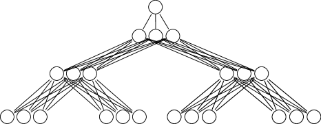
Figure 3: $G_{2,3}$ with $c=3$

To lower bound $\mathsf{\#BWpebbles}(G_{d,h})$, we will use Klawe’s result [Kla85]. Klawe showed that for “nice” graphs $G$, the black-white pebbling cost of $G$ (with black and white sliding moves) is at least $\lfloor\mathsf{\#pebbles}/2\rfloor+1$. Of course, the black-white pebbling cost without sliding moves is at least the cost with them. We define what it means for a graph to be nice in Klawe’s sense.

Definition 17

A DAG $G$ is nice if the following conditions hold:

1. If $u_{1}$, $u_{2}$ and $u$ are nodes of $G$ such that $u_{1}$ and $u_{2}$ are children of $u$ (i.e., there are edges from $u_{1}$ and $u_{2}$ to $u$), then the cost of black pebbling $u_{1}$ is equal to the cost of black pebbling $u_{2}$

2. If $u_{1}$ and $u_{2}$ are children of $u$, then there is no path from $u_{1}$ to $u_{2}$ or from $u_{2}$ to $u_{1}$.

3. If $u,u_{1},\ldots,u_{m}$ are nodes none of which has a path to another, then there are node-disjoint paths $P_{1},\ldots,P_{m}$ such that $P_{i}$ is a path from a leaf (a node with in-degree 0) to $u_{i}$ and there is no path between $u$ and any node in $P_{i}$.

$G_{d,h}$ is not nice in Klawe’s sense. We will delete some edges from $G_{d,h}$ to produce a nice graph $G^{\prime}_{d,h}$ and we will analyze $\mathsf{\#pebbles}(G^{\prime}_{d,h})$. Note that a lower bound on $\mathsf{\#BWpebbles}(G^{\prime}_{d,h})$ is also a lower bound on $\mathsf{\#BWpebbles}(G_{d,h})$.

The following definition will help in explaining the construction of $G^{\prime}_{d,h}$ as well as for specifying and proving properties of certain paths.

Definition 18

For $u\in G_{d,h}$, let $T_{d}^{h}(u)$ be the node in $T_{d}^{h}$ such that $T_{d}^{h}(u)[i]=u$ for some $i\leq c$. For $v,v^{\prime}\in T_{d}^{h}$, we say $v<v^{\prime}$ if $v$ is visited before $v^{\prime}$ in an inorder traversal of $T_{d}^{h}$. For $u,u^{\prime}\in G_{d,h}$, we say $u<u^{\prime}$ if $T_{d}^{h}(u)<T_{d}^{h}(u^{\prime})$ or if for some $v\in T_{d}^{h}$, $u=v[i]$, $u^{\prime}=v[j]$, and $i<j$.

$G_{d,h}^{\prime}$ is obtained from $G_{d,h}$ by removing $c-1$ edges from each internal node except the root, as follows (for an example, see figure 4). For each internal node $v$ of $T$, consider the corresponding nodes $v[1],v[2],\ldots,v[c]$ of $G_{d,h}$. Remove the edges from $v[i]$ to its $i-1$ smallest and $c-i$ largest children. So in the end each internal node except the root has $c(d-1)+1$ children.

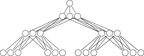
Figure 4: $G_{2,3}^{\prime}$ with $c=3$

We first analyze $\mathsf{\#pebbles}$($G^{\prime}_{d,h})$ and then show that it is nice. We show that $\mathsf{\#pebbles}(G_{d,h}^{\prime})=c[(d-1)(h-1)+1]$. Note that an upper bound of $c[(d-1)(h-1)+1]$ is attained using a simple recursive algorithm similar to that used for the binary tree.

For the lower bound, consider the earliest time $t$ when all paths from a leaf to the root are blocked. Figure 5 is an example of the type of pebbling configuration that we are about to analyze. The last pebble placed must have been placed at a leaf, since otherwise $t-1$ would be an earlier time when all paths from a leaf to the root are blocked. Let $P$ be the newly-blocked path from a leaf to the root. Consider the set $S=\{u\in G_{d,h}^{\prime}\ |\ u\not\in P\text{ and $u$ is a child of a node in }P\}$ of size $c(d-1)(h-1)+(c-1)=c[(d-1)(h-1)+1]-1$ (the $c-1$ is contributed by nodes at height $h$). We will give a set of mutually node-disjoint paths $\{P_{u}\}_{u\in S}$ such that $P_{u}$ is a path from a leaf to $u$ and $P_{u}$ does not intersect $P$. At time $t-1$, there must be at least one pebble on each $P_{u}$, since otherwise there would still be an open path from a leaf to the root at time $t$. Also counting the leaf node that is pebbled at $t$ gives c[(d-1)(h-1) + 1] pebbles.

Definition 19

The left-most (right-most) path to $u$ is the unique path ending at $u$ determined by choosing the smallest (largest) child at every level.

Definition 20

$P(l)$ is the node of path $P$ at height $l$, if it exists.

For each $u\in S$ at height $l$, if $u$ is less than (greater than) $P(l)$ then make $P_{u}$ the left-most (right-most) path to $u$. Now we need to show that the paths $\{P_{u}\}_{u\in S}\cup\{P\}$ are disjoint. The following fact is clear from the definition of $G_{d,h}^{\prime}$.

Lemma 21

For any $u,u^{\prime}\in G_{d,h}^{\prime}$, if $u<u^{\prime}$ then the smallest child of $u$ is not a child of $u^{\prime}$, and the largest child of $u^{\prime}$ is not a child of $u$.

First we show that $P_{u}$ and $P$ are disjoint. The following lemma will help now and in the proof that $G^{\prime}_{d,h}$ is nice.

Lemma 22

For $u,v\in G_{d,h}^{\prime}$ with $u<v$, if there is no path from $u$ to $v$ or from $v$ to $u$ then the left-most path to $u$ does not intersect any path to $v$ from a leaf, and the right-most path to $v$ does not intersect any path to $u$ from a leaf.

Proof:    Suppose otherwise and let $P_{u}^{\prime}$ be the left-most path to $u$, and $P_{v}^{\prime}$ a path to $v$ that intersects $P_{u}^{\prime}$. Since there is no path between $u$ and $v$, there is a height $l$, one greater than the height where the two paths first intersect, such that $P_{u}^{\prime}(l),P_{v}^{\prime}(l)$ are defined and $P_{u}^{\prime}(l)<P_{v}^{\prime}(l)$. But then from Lemma 21 $P_{u}^{\prime}(l-1)\not=P_{v}^{\prime}(l-1)$, a contradiction. The proof for the second part of the lemma is similar. $\blacksquare$

That $P_{u}$ and $P$ are disjoint follows from using Lemma 22 on $u$ and the sibling of $u$ in $P$.

Next we show that for distinct $u,u^{\prime}\in S$, $P_{u}$ does not contain $u^{\prime}$. Suppose it does. Assume $P_{u}$ is the left-most path to $u$ (the other case is similar). Since $u\not=u^{\prime}$, there must be a height $l$ such that $P_{u}(l)$ is defined and $P_{u}(l-1)=u^{\prime}$. From the definition of $S$, we know $P(l)$ is also a parent of $u^{\prime}$. From the construction of $P_{u}$, since we assumed $P_{u}$ is the left-most path to $u$, it must be that $P_{u}(l)<P(l)$. But then Lemma 21 tells us that $u^{\prime}$ cannot be a child of $P(l)$, a contradiction.

The proof that $P_{u}$ and $P_{u^{\prime}}$ do not intersect is by contradiction. Assuming that there are $u,u^{\prime}\in S$ such that $P_{u}$ and $P_{u^{\prime}}$ intersect, there is a height $l$, one greater than the height where they first intersect, such that $P_{u}(l)\not=P_{u^{\prime}}(l)$. Note that $P_{u}$ and $P_{u^{\prime}}$ are both left-most paths or both right-most paths, since otherwise in order for them to intersect they would need to cross $P$. But then from Lemma 21 $P_{u}(l-1)\not=P_{u^{\prime}}(l-1)$, a contradiction.

This is an example of a bottleneck of the specified structure for $G_{d,h}^{\prime}$ corresponding to the height 3 binary tree, with $c=3$:

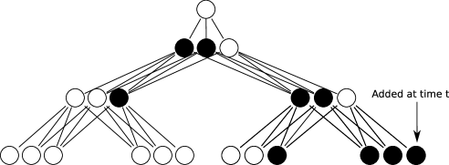
Figure 5: A possible black pebbling bottleneck of $G_{2,3}^{\prime}$, with $c=3$

The last step is to prove that $G_{d,h}^{\prime}$ is nice. There are three properties specified in Definition 17. Property 2 is obviously satisfied. For property 1, the argument used to give the black pebbling lower bound of $c[(d-1)(h-1)+1]$ can be used to give a black pebbling lower bound of $c(d-1)(l-1)+1$ for any node at height $l\leq h$ (the 1 is for the last node pebbled, and recall the root is at height $h+1$), and that bound is tight. For property 3, choose $P_{i}$ to be the left-most (right-most) path from $u_{i}$ if $u_{i}$ is less than (greater than) $u$. Then use Lemma 22 on each pair of nodes in $\{u,u_{1},\ldots,u_{m}\}$.

Since $\mathsf{\#pebbles}(G^{\prime}_{d,h})=c[(d-1)(h-1)+1]$, we have

$$\mathsf{\#BWpebbles}(G_{d,h})\geq\mathsf{\#BWpebbles}(G^{\prime}_{d,h})\geq c[(d-1)(h-1)+1]/2$$

and thus that the pebbling cost for the discretized game on $T_{d}^{h}$ is at least $(d-1)(h-1)/2+.5$, which implies $\mathsf{\#FRpebbles}(T_{d}^{h})\geq(d-1)(h-1)/2-.5$. $\blacksquare$

4.3 White sliding moves

In the definition of fractional pebbling (Definition 6) we allow black sliding moves but not white sliding moves. To allow white sliding moves we would add a clause

(iv) For every internal node $i$, if $w(i)=1$ and $j$ is a child of $i$ and every child of $i$ except $j$ has total pebble value 1, then decrease $w(i)$ to 0 and increase $w(j)$ so that node $j$ has total pebble value 1.

We did not include this move in the original definition because a nondeterministic $k$-way BP solving $FT_{d}^{h}(k)$ or $BT_{d}^{h}(k)$ does not naturally simulate it. The natural way to simulate such a move would be to verify the conjectured value of node $i$ (conjectured when the white pebble was placed on $i$) by comparing it with $f_{i}(v_{j_{1}},\ldots,v_{j_{d}})$, where $j_{1},\ldots,j_{d}$ are the children of $i$. But this would require the BP to remember a $(d+1)$-tuple of values, whereas potentially only $d$ pebbles are involved.

White sliding moves definitely reduce the number of pebbles required to pebble some trees. For example the binary tree $T^{3}_{2}$ can easily be pebbled with 2 pebbles using white sliding moves, but requires 2.5 pebbles without (Theorem 15). The next result shows that $8/3$ pebbles suffice for pebbling $T^{4}_{2}$ with white sliding moves, whereas 3 pebbles are required without (Theorem 15).

Theorem 23

The binary tree of height 4 can be pebbled with $8/3$ pebbles using white sliding moves.

Proof:    The height 3 binary tree can be pebbled with 2 pebbles. Use that sequence on node 2, but leave a third black pebble on node 2. That takes 7/3 pebbles. Put black pebbles on nodes 12 and 13. Slide a third black pebble up to node 6. Remove the pebbles on nodes 12 and 13. Put black pebbles on nodes 14 and 15 – this is the first configuration with 8/3 pebbles. Slide the pebble on node 14 up to node 7. Remove the pebble from 15. Put 2/3 of a white pebble on node 6. Slide the black pebble on node 7 up to node 3. Remove a third black pebble from node 6. Put 2/3 of a white pebble on node 2 – the resulting configuration has 8/3 pebbles. Slide the black pebble on node 3 up to the root. Remove all black pebbles. At this point there is 2/3 of a white pebble on both node 2 and node 6. Put a black pebble on node 12 and a third black pebble on node 13 – another bottleneck. Slide the 2/3 white pebble on node 6 down to node 13. Remove the pebbles from nodes 12 and 13. Finally, use 8/3 pebbles to remove the 2/3 white pebble from node 2. $\blacksquare$

5 Branching Program Bounds

In this section we prove tight bounds (up to a constant factor) for the number of states required for both deterministic and nondeterministic $k$-way branching programs to solve the Boolean problems $BT_{d}^{3}(k)$ for all trees of height 2 and 3. (The bound is obviously $\Theta(k^{d})$ for trees of height 2, because there are $d+k^{d}$ input variables.) For every height $h\geq 2$ we prove upper bounds for deterministic thrifty programs which solve $FT_{d}^{h}(k)$ (Theorem 24, (14)), and show that these bounds are optimal for degree $d=2$ even for the Boolean problem $BT_{d}^{h}(k)$ (Theorem 33). We prove upper bounds for nondeterministic thrifty programs solving $BT_{d}^{h}(k)$ in general, and show that these are optimal for binary trees of height 4 or less (Theorems 24 and 37).

For the nondeterministic case our best BP upper bounds for every $h\geq 2$ come from fractional pebbling algorithms via Theorem 10. For the deterministic case our best bounds for the function problem $FT_{d}^{h}(k)$ come from black pebbling via the same theorem, although we can improve on them for the Boolean problem $BT_{2}^{h}(k)$ by a factor of $\log k$ (for $h\geq 3)$.

Theorem 24 (BP Upper Bounds)

For all $h,d\geq 2$

$$\mathsf{\#detFstates}^{h}_{d}(k) = O(k^{(d-1)h-d+2})$$ (14)

$$\mathsf{\#detBstates}^{h}_{d}(k) = O(k^{(d-1)h-d+2}/\log k),\mbox{ for $h\geq 3$}$$ (15)

$$\mathsf{\#ndetBstates}^{h}_{d}(k) = O(k^{(d-1)(h/2)+1})$$ (16)

The first and third bounds are realized by thrifty programs.

Proof:    The first and third bounds follow from Theorem 10 (which states that pebbling upper bounds give rise to upper bounds for the size of thrifty BPs) and from Theorems 12 and 15 (which give the required pebbling upper bounds).

To prove (15) we use a branching program which implements the algorithm below. Here we have a parameter $m$, and choosing $m=\lceil\log k^{d-1}-\log\log k^{d-1}\rceil$ suffices to show $\mathsf{\#detBstates}^{h}_{d}(k)=O(k^{(d-1)(h-1)+1}/\log k^{d-1})$, from which (15) follows. We estimate the number of states required up to a constant factor.

1) Compute $v_{2}$ (the value of node 2 in the heap ordering), using the black pebbling algorithm for the principal left subtree. This requires $k^{(d-1)(h-2)+1}$ states. Divide the $k$ possible values for $v_{2}$ into $\lceil k/m\rceil$ blocks of size $m$.

2) Remember the block number for $v_{2}$, and compute $v_{3},\ldots,v_{d+1}$. This requires $k/m\times k^{d-2}\times k^{(d-1)(h-2)+1}=k^{(d-1)(h-1)+1}/m$ states.

3) Remember $v_{3},\ldots,v_{d+1}$ and the block number for $v_{2}$. Compute $f_{1}(a,v_{3},\ldots,v_{d+1})$ for each of the $m$ possible values $a$ for $v_{2}$ in its block number, and keep track of the set of $a$’s for which $f_{1}=1$. This requires $k^{d-1}\times k/m\times m\times 2^{m}=k^{d}2^{m}$ states.

4) Remember just the set of possible $a$’s (within its block) from above (there are $2^{m}$ possibilities). Compute $v_{2}$ again and accept or reject depending on whether $v_{2}$ is in the subset. This requires $k^{(d-1)(h-2)+1}2^{m}$ states.

The total number of states has order the maximum of $k^{(d-1)(h-1)+1}/m$ and $k^{(d-1)(h-2)+1}2^{m}$, which is at most

$$k^{(d-1)(h-1)+1}/(\log k^{d-1}-\log\log k^{d-1})$$

for $m=\log k^{d-1}-\log\log k^{d-1}$. $\blacksquare$

We combine the above upper bounds with the Nec̆iporuk lower bounds in Subsection 5.1, Figure 6, to obtain the following.

Corollary 25 (Tight bounds for height 3 trees)

For all $d\geq 2$

$$\mathsf{\#detFstates}^{3}_{d}(k) = \Theta(k^{2d-1})$$

$$\mathsf{\#detBstates}^{3}_{d}(k) = \Theta(k^{2d-1}/\log k)$$

$$\mathsf{\#ndetBstates}^{3}_{d}(k) = \Theta(k^{(3/2)d-1/2})$$

5.1 The Nec̆iporuk method

The Nec̆iporuk method still yields the strongest explicit binary branching program size lower bounds known today, namely $\Omega(\frac{n^{2}}{(\log n)^{2}})$ for deterministic [Nec̆66] and $\Omega(\frac{n^{3/2}}{\log n})$ for nondeterministic (albeit for a weaker nondeterministic model in which states have bounded outdegree [Pud87], see [Raz91]).

By applying the Nec̆iporuk method to a $k$-way branching program $B$ computing a function $f:[k]^{m}\rightarrow R$, we mean the following well known steps [Nec̆66]:

1. Upper bound the number $N(s,v)$ of (syntactically) distinct branching programs of type $B$ having $s$ non-final states, each labelled by one of $v$ variables.

2. Pick a partition $\{V_{1},\ldots,V_{p}\}$ of $[m]$.

3. For $1\leq i\leq p$, lower bound the number $r_{V_{i}}(f)$ of restrictions $f_{V_{i}}:[k]^{|V_{i}|}\rightarrow R$ of $f$ obtainable by fixing values of the variables in $[m]\setminus V_{i}$.

4. Then size($B$) $\geq$ $|R|+\sum_{1\leq i\leq p}s_{i}$, where $s_{i}=\min\{\ s:N(s,|V_{i}|)\geq r_{V_{i}}(f)\ \}$.

Theorem 26

Applying the Nec̆iporuk method yields Figure 6.

Model	Lower bound for $FT_{d}^{h}(k)$	Lower bound for $BT_{d}^{h}(k)$
Deterministic $k$-way branching program	$\frac{d^{h-2}-1}{4(d-1)^{2}}\cdot k^{2d-1}$	$\frac{d^{h-2}-1}{3(d-1)^{2}}\cdot\frac{k^{2d-1}}{\log k}$
Deterministic binary branching program	$\frac{d^{h-2}-1}{5(d-1)^{2}}\cdot k^{2d}=\Omega(n^{2}/(\log n)^{2})$	$\frac{d^{h-2}-1}{4d(d-1)}\cdot\frac{k^{2d}}{\log k}=\Omega(n^{2}/(\log n)^{3})$
Nondeterministic $k$-way BP	$\frac{d^{h-2}-1}{2d-2}\cdot k^{\frac{3d}{2}-\frac{1}{2}}\sqrt{\log k}$	$\frac{d^{h-2}-1}{2d-2}\cdot k^{\frac{3d}{2}-\frac{1}{2}}$
Nondeterministic binary BP	$\frac{d^{h-2}-1}{2d-2}\cdot k^{\frac{3d}{2}}\sqrt{\log k}=\Omega(n^{3/2}/\log n)$	$\frac{d^{h-2}-1}{2d-2}\cdot k^{\frac{3d}{2}}=\Omega(n^{3/2}/(\log n)^{3/2})$

Figure 6: Size bounds, expressed in terms of $n=\Theta(k^{d}\log k)$ in the binary cases, obtained by applying the Nec̆iporuk method. Rectangles indicate optimality in $k$ when $h=3$ (Cor. 25). Improving any entry to $\Omega(k^{\mbox{\scriptsize unbounded }f(h)})$ would prove $\mathbf{L}\subsetneq\mathbf{P}$ (Cor. 9).

• The $\Omega(n^{3/2}/(\log n)^{3/2})$ binary nondeterministic BP lower bound for the $BT_{d}^{h}(k)$ problem and in particular for $BT_{2}^{3}(k)$ applies to the number of states when these can have arbitrary outdegree. This seems to improve on the best known former bound of $\Omega(n^{3/2}/\log n)$, slightly larger but obtained for the weaker model in which states have bounded degree, or equivalently, for the switching and rectifier network model in which size is defined as the number of edges [Pud87, Raz91].

Proof:   [Proof of Theorem 26] We have $N_{\mbox{\scriptsize det}}^{\mbox{\scriptsize$k$-way}}(s,v)\leq v^{s}\cdot(s+|R|)^{sk}$ for the number of deterministic BPs and $N_{\mbox{\scriptsize nondet}}^{\mbox{\scriptsize$k$-way}}(s,v)\leq v^{s}\cdot(|R|+1)^{sk}\cdot(2^{s})^{sk}$ for nondeterministic BPs having $s$ non-final states, each labelled with one of $v$ variables. To see $N_{\mbox{\scriptsize nondet}}^{\mbox{\scriptsize$k$-way}}(s,v)$, note that edges labelled $i\in[k]$ can connect a state $S$ to zero or one state among the final states and can connect $S$ independently to any number of states among the non-final states.

The only decision to make when applying the Nec̆iporuk method is the choice of the partition of the input variables. Here every entry in Figure 6 is obtained using the same partition (with the proviso that a $k$-ary variable in the partition is replaced by $\log k$ binary variables when we treat $2$-way branching programs).

We will only partition the set $V$ of $k$-ary $FT_{d}^{h}(k)$ or $BT_{d}^{h}(k)$ variables that pertain to internal tree nodes other than the root (we will neglect the root and leaf variables). Each internal tree node has $d-1$ siblings and each sibling involves $k^{d}$ variables. By a litter we will mean any set of $d$ $k$-ary variables that pertain to precisely $d$ such siblings. We obtain our partition by writing $V$ as a union of

$$k^{d}\cdot\Sigma_{i=0}^{h-3}d^{i}=k^{d}\cdot\frac{d^{h-2}-1}{d-1}$$

litters. (Specifically, each litter can be defined as

$$\{f_{i}(j_{1},j_{2},\ldots,j_{d}),f_{i+1}(j_{1},j_{2},\ldots,j_{d}),\ldots,f_{i+d-1}(j_{1},j_{2},\ldots,j_{d})\}$$

for some $1\leq j_{1},j_{2},\ldots,j_{d}\leq k$ and some $d$ siblings $i,i+1,\ldots,i+d-1$.)

Consider such a litter $L$. We claim that $|R|^{k^{d}}$ distinct functions $f_{L}:[k]^{d}\rightarrow R$ can be induced by setting the variables outside of $L$, where $|R|=k$ in the case of $FT_{d}^{h}(k)$ and $|R|=2$ in the case of $BT_{d}^{h}(k)$. Indeed, to induce any such function, fix the “descendants of the litter $L$” to make each variable in $L$ relevant to the output; then, set the variables pertaining to the immediate ancestor node $\nu$ of the siblings forming $L$ to the appropriate $k^{d}$ values, as if those were the final output desired; finally, set all the remaining variables in a way such that the values in $\nu$ percolate from $\nu$ to the root.

It remains to do the calculations. We illustrate two cases. Similar calculations yield the other entries in Figure 6.

Nondeterministic $k$-way branching programs computing $FT_{d}^{h}(k)$. Here $|R|=k$. In a correct program, the number $s$ of states querying one of the $d$ litter $L$ variables must satisfy

$$k^{k^{d}}\leq N_{\mbox{\scriptsize nondet}}^{\mbox{\scriptsize$k$-way}}(s,d)\leq d^{s}\cdot(k+1)^{sk}\cdot(2^{s})^{sk}\leq s^{s}\cdot k^{2sk}\cdot(2^{s})^{sk}$$

since $d\leq s$ (because $FT_{d}^{h}(k)$ depends on all its variables), and thus

$$k^{d}\log k\leq s(\log s+2k\log k)+s^{2}k.$$

Suppose to the contrary that $s<(k^{\frac{d-1}{2}}\sqrt{\log k})/2$. Then

$$s(\log s+2k\log k)+s^{2}k<s(\frac{d-1}{2}\log k+\frac{\log\log k}{2}+2k\log k)+s^{2}k<s(sk)+s^{2}k<k^{d}\log k$$

for large $k$ and all $d\geq 2$, a contradiction. Hence $s\geq(k^{\frac{d-1}{2}}\sqrt{\log k})/2$. Since this holds for every litter, recalling step 4 in the Nec̆iporuk method as described prior to Theorem 26, the total number of states in the program is at least

$$k+k^{d}\cdot\frac{d^{h-2}-1}{d-1}\cdot(k^{\frac{d-1}{2}}\sqrt{\log k})/2\geq\frac{d^{h-2}-1}{2d-2}\cdot k^{\frac{3d}{2}-\frac{1}{2}}\sqrt{\log k}.$$

Nondeterministic binary (ie $2$-way) branching programs deciding $BT_{d}^{h}(k)$. Here $|R|=2$. When the program is binary, the $d$ variables in the litter $L$ become $d\log k$ Boolean variables. The number $s$ of states querying one of these $d\log k$ variables then verifies

$$2^{k^{d}}\leq N_{\mbox{\scriptsize nondet}}^{\mbox{\scriptsize$2$-way}}(s,d\log k)\leq(d\log k)^{s}\cdot(2+1)^{2s}\cdot(2^{s})^{2s}<(s\log k)^{s}\cdot 2^{4s+2s^{2}}$$

since $d\leq s$ and thus

$$k^{d}\leq s\log s+s\log\log k+4s+2s^{2}\leq 3s^{2}+5s\log\log k.$$

It follows that $s\geq k^{\frac{d}{2}}/2$. Hence the total number of states in a binary nondeterministic program deciding $BT_{d}^{h}(k)$ is at least

$$k^{d}\cdot\frac{d^{h-2}-1}{d-1}\cdot\frac{k^{d/2}}{2}\geq\frac{d^{h-2}-1}{2(d-1)}\cdot k^{\frac{3d}{2}}=\frac{d^{h-2}-1}{2(d-1)}\cdot\frac{(k^{d}\log k)^{3/2}}{(\log k)^{3/2}}=\Omega(n^{3/2}/(\log n)^{3/2})$$

where $n=\Theta(k^{d}\log k)$ is the length of the binary encoding of $BT_{d}^{h}(k)$. $\blacksquare$

The next two results show limitations on the Nec̆iporuk method that are not necessarily present in the state sequence method (see Theorems 31 and 32).

Let $Children_{d}^{h}(k)$ have the same input as $FT_{d}^{h}(k)$ with the exception that the root function is deleted. The output is the tuple $(v_{2},v_{3},\ldots,v_{d+1})$ of values for the children of the root. $Children_{d}^{h}(k)$ can be computed by a $k$-way deterministic BP with $O(k^{(d-1)h-d+2})$ states using the same black pebbling method which yields the bound (14) in Theorem 24.

Theorem 27

For any $d,h\geq 2$, the best $k$-way deterministic BP size lower bound attainable for $Children_{d}^{h}(k)$ by applying the Nec̆iporuk method is $\Omega(k^{2d-1})$.

Proof:    The function $Children_{d}^{h}(k):[k]^{m}\rightarrow R$ has $m=\Theta(k^{d})$. Any partition $\{V_{1},\ldots,V_{p}\}$ of the set of $k$-ary input variables thus has $p=O(k^{d})$. Claim: for each $i$, the best attainable lower bound on the number of states querying variables from $V_{i}$ is $O(k^{d-1})$.

Consider such a set $V_{i}$, $|V_{i}|=v\geq 1$. Here $|R|=k^{d}$, so the number $N_{\mbox{\scriptsize det}}^{\mbox{\scriptsize$k$-way}}(s,v)$ of distinct deterministic BPs having $s$ non-final states querying variables from $V_{i}$ satisfies

$$N_{\mbox{\scriptsize det}}^{\mbox{\scriptsize$k$-way}}(s,v)\geq 1^{s}\cdot(s+|R|)^{sk}\geq(1+k^{d})^{sk}\geq k^{dsk}.$$

Hence the estimate used in the Nec̆iporuk method to upper bound $N_{\mbox{\scriptsize det}}^{\mbox{\scriptsize$k$-way}}(s,v)$ will be at least $k^{dsk}$. On the other hand, the number of functions $f_{V_{i}}:[k]^{v}\rightarrow R$ obtained by fixing variables outside of $V_{i}$ cannot exceed $k^{O(k^{d})}$ since the number of variables outside $V_{i}$ is $\Theta(k^{d})$. Hence the best lower bound on the number of states querying variables from $V_{i}$ obtained by applying the method will be no larger than the smallest $s$ verifying $k^{ck^{d}}\leq k^{dsk}$ for some $c$ depending on $d$ and $k$. This proves our claim since then this number is at most $s=O(k^{d-1})$. $\blacksquare$

Let $\mathit{SumMod}_{d}^{h}(k)$ have the same input as $FT_{d}^{h}(k)$ with the exception that the root function is preset to the sum modulo $k$. In other words the output is $v_{2}+v_{3}+\cdots+v_{d+1}\mod k$.

Theorem 28

The best $k$-way deterministic BP size lower bound attainable for $\mathit{SumMod}_{2}^{3}(k)$ by applying the Nec̆iporuk method is $\Omega(k^{2})$.

Proof:    The function $\mathit{SumMod}_{2}^{3}(k):[k]^{m}\rightarrow R$ has $m=\Theta(k^{2})$. Consider a set $V_{i}$ in any partition $\{V_{1},\ldots,V_{p}\}$ of the set of $k$-ary input variables, $|V_{i}|=v$. Here $|R|=k$, so the number $N_{\mbox{\scriptsize det}}^{\mbox{\scriptsize$k$-way}}(s,v)$ of distinct deterministic BPs having $s$ non-sink states querying variables from $V_{i}$ satisfies

$$N_{\mbox{\scriptsize det}}^{\mbox{\scriptsize$k$-way}}(s,v)\geq 1^{s}\cdot(s+|R|)^{sk}\geq(1+k)^{sk}\geq k^{sk}.$$

If $V_{i}$ contains a leaf variable, then perhaps the number of functions induced by setting variables complementary to $V_{i}$ can reach the maximum $k^{k^{2}}$. Nec̆iporuk would conclude that $k$ states querying the variables from such a $V_{i}$ are necessary. Note that there are at most $4$ sets $V_{i}$ containing a leaf variable (hence a total of $4k$ states required to account for the variables in these $4$ sets). Now suppose that $V_{i}$ does not contain a leaf variable. Then setting the variables complementary to $V_{i}$ can either induce a constant function (there are $k$ of those), or the sum of a constant plus a variable (there are at most $k\cdot|V_{i}|$ of those) or the sum of two of the variables (there are at most $|V_{i}|^{2}$ of those). So the maximum number of induced functions is $|V_{i}|^{2}=O(k^{4})$. The number of states querying variables from $V_{i}$ is found by Nec̆iporuk to be $s\geq 4/k$. In other words $s=1$. So for any of the at least $p-4$ sets in the partition not containing a leaf variable, the method gets one state. Since $p-4=O(k^{2})$, the total number of states accounting for all the $V_{i}$ is $O(k^{2})$. $\blacksquare$

5.2 The state sequence method

Here we give alternative proofs for some of the lower bounds given in Section 5.1. These proofs are more intricate than the Nec̆iporuk proofs but they do not suffer a priori from a quadratic limitation. The method also yields stronger lower bounds for $Children_{2}^{4}(k)$ and $\mathit{SumMod}_{2}^{3}(k)$ (Theorems 31 and 32) than those obtained by applying Nec̆iporuk’s method (Theorems 27 and 28).

Theorem 29

$\mathsf{\#ndetBstates}^{3}_{2}(k)\geq k^{2.5}$ for sufficiently large $k$.

Proof:    Consider an input $I$ to $BT_{2}^{3}(k)$. We number the nodes in $T^{3}_{2}$ as in Figure 1, and let $v^{I}_{j}$ denote the value of node $j$ under input $I$. We say that a state in a computation on input $I$ learns $v^{I}_{j}$ if that state queries $f_{j}^{I}(v^{I}_{2j},v^{I}_{2j+1})$ (recall $2j,2j+1$ are the children of node $j$).

Definition [Learning Interval] Let $B$ be a $k$-way nondeterministic BP that solves $BT_{2}^{3}(k)$. Let ${\cal C}=\gamma_{0},\gamma_{1},\cdots,\gamma_{T}$ be a computation of $B$ on input $I$. We say that a state $\gamma_{i}$ in the computation is critical if one or more of the following holds:

1. $i=0$ or $i=T$

2. $\gamma_{i}$ learns $v^{I}_{2}$ and there is an earlier state which learns $v^{I}_{3}$ with no intervening state that learns $v^{I}_{2}$.

3. $\gamma_{i}$ learns $v^{I}_{3}$ and no earlier state learns $v^{I}_{3}$ unless an intervening state learns $v^{I}_{2}$.

We say that a subsequence $\gamma_{i},\gamma_{i+1},\cdots\gamma_{j}$ is a learning interval if $\gamma_{i}$ and $\gamma_{j}$ are consecutive critical states. The interval is type 3 if $\gamma_{i}$ learns $v^{I}_{3}$, and otherwise the interval is type 2.

Thus type 2 learning intervals begin with $\gamma_{0}$ or a state which learns $v^{I}_{2}$, and never learn $v^{I}_{3}$ until the last state, and type 3 learning intervals begin with a state which learns $v^{I}_{3}$ and never learn $v^{I}_{2}$ until the last state.

Now let $B$ be as above, and for $j\in\{2,3\}$ let $\Gamma_{j}$ be the set of all states of $B$ which query the input function $f_{j}$. We will prove the theorem by showing that for large $k$

$$|\Gamma_{2}|+|\Gamma_{3}|>k^{2}\sqrt{k}.$$ (17)

For $r,s\in[k]$ let $F^{r,s}_{yes}$ be the set of inputs $I$ to $B$ whose four leaves are labelled $r,s,r,s$ respectively, whose middle node functions $f_{2}^{I}$ and $f_{3}^{I}$ are identically 1 except $f^{I}_{2}(r,s)=v^{I}_{2}$ and $f^{I}_{3}(r,s)=v^{I}_{3}$, and $f^{I}_{1}(v^{I}_{2},v^{I}_{3})=1$ (so $v^{I}_{1}=1$). Thus each such $I$ is a ‘YES input’, and should be accepted by $B$.

Note that each member $I$ of $F_{yes}^{r,s}$ is uniquely specified by a triple

$$(v^{I}_{2},v^{I}_{3},f^{I}_{1})\mbox{ where $f^{I}_{1}(v^{I}_{2},v^{I}_{3})=1$}$$ (18)

and hence $F_{yes}^{r,s}$ has exactly $k^{2}(2^{k^{2}-1})$ members.

For $j\in\{2,3\}$ and $r,s\in[k]$ let $\Gamma_{j}^{r,s}$ be the subset of $\Gamma_{j}$ consisting of those states which query $f_{j}(r,s)$. Then $\Gamma_{j}$ is the disjoint union of $\Gamma_{j}^{r,s}$ over all pairs $(r,s)$ in $[k]\times[k]$. Hence to prove (17) it suffices to show

$$|\Gamma_{2}^{r,s}|+|\Gamma_{3}^{r,s}|>\sqrt{k}$$ (19)

for large $k$ and all $r,s$ in $[k]$. We will show this by showing

$$(|\Gamma_{2}^{r,s}|+1)(|\Gamma_{3}^{r,s}|+1)\geq k/2$$ (20)

for all $k\geq 2$. (Note that given the product, the sum is minimized when the summands are equal.)

For each input $I$ in $F_{yes}^{r,s}$ we associate a fixed accepting computation ${\cal C}(I)$ of $B$ on input $I$.

Now fix $r,s\in[k]$. For $a,b\in[k]$ and $f:[k]\times[k]\rightarrow\{0,1\}$ with $f(a,b)=1$ we use $(a,b,f)$ to denote the input $I$ in $F_{yes}^{r,s}$ it represents as in (18).

To prove (20), the idea is that if it is false, then as $I$ varies through all inputs $(a,b,f)$ in $F_{yes}^{r,s}$ there are too few states learning $v^{I}_{2}=a$ and $v^{I}_{3}=b$ to verify that $f(a,b)=1$. Specifically, we can find $a,b,f,g$ such that $f(a,b)=1$ and $g(a,b)=0$, and by cutting and pasting the accepting computation ${\cal C}(a,b,f)$ with accepting computations of the form ${\cal C}(a,b^{\prime},g)$ and ${\cal C}(a^{\prime},b,g)$ we can construct an accepting computation of the ‘NO input’ $(a,b,g)$.

We may assume that the branching program $B$ has a unique initial state $\gamma_{0}$ and a unique accepting state $\delta_{ACC}$.

For $j\in\{2,3\}$, $a,b\in[k]$ and $f:[k]\times[k]\rightarrow\{0,1\}$ with $f(a,b)=1$ define $\varphi_{j}(a,b,f)$ to be the set of all state pairs $(\gamma,\delta)$ such that there is a type $j$ learning interval in ${\cal C}(a,b,f)$ which begins with $\gamma$ and ends with $\delta$. Note that if $j=2$ then $\gamma\in(\Gamma_{2}^{r,s}\cup\{\gamma_{0}\})$ and $\delta\in(\Gamma_{3}^{r,s}\cup\{\delta_{ACC}\})$, and if $j=3$ then $\gamma\in\Gamma_{3}^{r,s}$ and $\delta\in(\Gamma_{2}^{r,s}\cup\{\delta_{ACC}\})$.

To complete the definition, define $\varphi_{j}(a,b,f)=\varnothing$ if $f(a,b)=0$.

For $j\in\{2,3\}$ and $f:[k]\times[k]\rightarrow\{0,1\}$ we define a function $\varphi_{j}[f]$ from $[k]$ to sets of state pairs as follows:

$$\varphi_{2}[f](a) = \bigcup_{b\in[k]}\varphi_{2}(a,b,f)\ \subseteq S_{2}$$

$$\varphi_{3}[f](b) = \bigcup_{a\in[k]}\varphi_{3}(a,b,f)\ \subseteq S_{3}$$

where $S_{2}=(\Gamma_{2}^{r,s}\cup\{\gamma_{0}\})\times(\Gamma_{3}^{r,s}\cup\{\delta_{ACC}\})$ and $S_{3}=\Gamma_{3}^{r,s}\times(\Gamma_{2}^{r,s}\cup\{\delta_{ACC}\})$.

For each $f$ the function $\varphi_{j}[f]$ can be specified by listing a $k$-tuple of subsets of $S_{j}$, and hence there are at most $2^{k|S_{j}|}$ distinct such functions as $f$ ranges over the $2^{k^{2}}$ Boolean functions on $[k]\times[k]$, and hence there are at most $2^{k(|S_{2}|+|S_{3}|)}$ pairs of functions $(\varphi_{2}[f],\varphi_{3}[f])$. If we assume that (20) is false, we have $|S_{2}|+|S_{3}|<k$. Hence by the pigeonhole principle there must exist distinct Boolean functions $f,g$ such that $\varphi_{2}[f]=\varphi_{2}[g]$ and $\varphi_{3}[f]=\varphi_{3}[g]$.

Since $f$ and $g$ are distinct we may assume that there exist $a,b$ such that $f(a,b)=1$ and $g(a,b)=0$. Since $\varphi_{2}[f](a)=\varphi_{2}[g](a)$, if $(\gamma,\delta)$ are the endpoints of a type 2 learning interval in ${\cal C}(a,b,f)$ there exists $b^{\prime}$ such that $(\gamma,\delta)$ are the endpoints of a type 2 learning interval in ${\cal C}(a,b^{\prime},g)$ (and hence $g(a,b^{\prime})=1$). Similarly, if $(\gamma,\delta)$ are endpoints of a type 3 learning interval in ${\cal C}(a,b,f)$ there exists $a^{\prime}$ such that $(\gamma,\delta)$ are the endpoints of a type 3 learning interval in ${\cal C}(a^{\prime},b,f)$.

Now we can construct an accepting computation for the ‘NO input’ $(a,b,g)$ from ${\cal C}(a,b,f)$ by replacing each learning interval beginning with some $\gamma$ and ending with some $\delta$ by the corresponding learning interval in ${\cal C}(a,b^{\prime},g)$ or ${\cal C}(a^{\prime},b,g)$. (The new accepting computation has the same sequence of critical states as ${\cal C}(a,b,f)$.) This works because a type 2 learning interval never queries $v_{3}$ and a type 3 learning interval never queries $v_{2}$.

This completes the proof of (20) and the theorem. $\blacksquare$

Theorem 30

Every deterministic branching program that solves $BT_{2}^{3}(k)$ has at least $k^{3}/\log k$ states for sufficiently large $k$.

Proof:    We modify the proof of Theorem 29. Let $B$ be a deterministic BP which solves $BT_{2}^{3}(k)$, and for $j\in\{2,3\}$ let $\Gamma_{j}$ be the set of states in $B$ which query $f_{j}$ (as before). It suffices to show that for sufficiently large $k$

$$|\Gamma_{2}|+|\Gamma_{3}|\geq k^{3}/\log k.$$ (21)

For $r,s\in[k]$ we define the set $F^{r,s}$ to be the same as $F_{yes}^{r,s}$ except that we remove the restriction on $f^{I}_{1}$. Hence there are exactly $k^{2}2^{k^{2}}$ inputs in $F^{r,s}$.

As before, for $j\in\{2,3\}$, $\Gamma_{j}$ is the disjoint union of $\Gamma^{r,s}$ for $r,s\in[k]$. Thus to prove (21) it suffices to show that for sufficiently large $k$ and all $r,s$ in $[k]$

$$|\Gamma_{2}^{r,s}|+|\Gamma_{3}^{r,s}|\geq k/\log k.$$ (22)

We may assume there are unique start, accepting, and rejecting states $\gamma_{0}$, $\delta_{ACC}$, $\delta_{REJ}$. Fix $r,s\in[k]$.

For each root function $f:[k]\times[k]\rightarrow\{0,1\}$ we define the functions

$$\psi_{2}[f]:[k]\times(\Gamma_{2}^{r,s}\cup\{\gamma_{0}\}) \rightarrow (\Gamma_{3}^{r,s}\cup\{\delta_{ACC},\delta_{REJ}\})$$

$$\psi_{3}[f]:[k]\times\Gamma_{3}^{r,s} \rightarrow (\Gamma_{2}^{r,s}\cup\{\delta_{ACC},\delta_{REJ}\})$$

by $\psi_{2}[f](a,\gamma)=\delta$ if $\delta$ is the next critical state after $\gamma$ in a computation with input $(a,b,f)$ (this is independent of $b$), or $\delta=\delta_{REJ}$ if there is no such critical state. Similarly $\psi_{3}[f](b,\delta)=\gamma$ if $\gamma$ is the next critical state after $\delta$ in a computation with input $(a,b,f)$ (this is independent of $a$), or $\delta=\delta_{REJ}$ if there is no such critical state.

CLAIM: The pair of functions $(\psi_{2}[f],\psi_{3}[f])$ is distinct for distinct $f$.

For suppose otherwise. Then there are $f,g$ such that $\psi_{2}[f]=\psi_{2}[g]$ and $\psi_{3}[f]=\psi_{3}[g]$ but $f(a,b)\neq g(a,b)$ for some $a,b$. But then the sequences of critical states in the two computations $C(a,b,f)$ and $C(a,b,g)$ must be the same, and hence the computations either accept both $(a,b,f)$ and $(a,b,g)$ or reject both. So the computations cannot both be correct.

Finally we prove (22) from the CLAIM. Let $s_{2}=|\Gamma_{2}^{r,s}|$ and let $s_{3}=|\Gamma_{3}^{r,s}|$, and let $s=s_{2}+s_{3}$. Then the number of distinct pairs $(\psi_{2},\psi_{3})$ is at most

$$(s_{3}+2)^{k(s_{2}+1)}(s_{2}+2)^{ks_{3}}\leq(s+2)^{k(s+1)}$$

and since there are $2^{k^{2}}$ functions $f$ we have

$$2^{k^{2}}\leq(s+2)^{k(s+1)}$$

so taking logs, $k^{2}\leq k(s+1)\log(s+2)$ so $k/\log(s+2)\leq s+1$, and (22) follows. $\blacksquare$

Recall from Theorem 27 that applying the Nec̆iporuk method to $Children_{2}^{4}(k)$ yields an $\Omega(k^{3})$ size lower bound and from Theorem 28 that applying it to $\mathit{SumMod}_{2}^{3}(k)$ yields $\Omega(k^{2})$. The next two results improve on these bounds using the state sequence method. The new lower bounds match the upper bounds given by the pebbling method used to prove (14) in Theorem 24.

Theorem 31

Any deterministic $k$-way BP for $Children_{2}^{4}(k)$ has at least $k^{4}/2$ states.

Proof:    Let $E_{4true}$ be the set of all inputs $I$ to $Children_{2}^{4}(k)$ such that $f_{2}^{I}=f^{I}_{3}=+_{k}$ (addition mod $k$), and for $i\in\{4,5,6,7\}$ $f^{I}_{i}$ is identically 0 except for $f^{I}_{i}(v^{I}_{2i},v^{I}_{2i+1})$.

Let $B$ be a branching program as in the theorem. For each $I\in E_{4true}$ let ${\cal C}(I)$ be the computation of $B$ on input $I$.

For $r,s\in[k]$ let $E^{r,s}_{4true}$ be the set of inputs $I$ in $E_{4true}$ such that for $i\in\{4,5,6,7\}$, $v^{I}_{2i}=r$ and $v^{I}_{2i+1}=s$. Then for each pair $r,s$ each input $I$ in $E^{r,s}_{4true}$ is completely specified by the quadruple $v^{I}_{4},v^{I}_{5},v^{I}_{6},v^{I}_{7}$, so $|E^{r,s}_{4true}|=k^{4}$.

For $r,s\in[k]$ and $i\in\{4,5,6,7\}$ let $\Gamma^{r,s}_{i}$ be the set of states of $B$ that query $f_{i}(r,s)$, and let

$$\Gamma^{r,s}=\Gamma^{r,s}_{4}\cup\Gamma^{r,s}_{5}\cup\Gamma^{r,s}_{6}\cup\Gamma^{r,s}_{7}$$ (23)

The theorem follows from the following Claim.

CLAIM 1: $|\Gamma^{r,s}|\geq k^{2}/2$ for all $r,s\in[k]$.

To prove CLAIM 1, suppose to the contrary for some $r,s$

$$|\Gamma^{r,s}|<k^{2}/2$$ (24)

We associate a pair

$$T(I)=(\gamma^{I},v^{I}_{i})$$

with $I$ as follows: $\gamma^{I}$ is the last state in the computation ${\cal C}(I)$ that is in $\Gamma^{r,s}$ (such a state clearly exists), and $i\in\{4,5,6,7\}$ is the node queried by $\gamma^{I}$. (Here $v^{I}_{i}$ is the value of node $i$).

We also associate a second triple $U(I)$ with each input $I$ in $E^{r,s}_{4true}$ as follows:

$$U(I)=\left\{\begin{array}[]{ll}(v^{I}_{4},v^{I}_{5},v^{I}_{3})&\mbox{if $\gamma^{I}$ queries node 4 or 5 }\\ (v^{I}_{6},v^{I}_{7},v^{I}_{2})&\mbox{otherwise.}\end{array}\right.$$

CLAIM 2: As $I$ ranges over $E^{r,s}_{4true}$, $U(I)$ ranges over at least $k^{3}/2$ triples in $[k]^{3}$.

To prove CLAIM 2, consider the the subset $E^{\prime}$ of inputs in $E^{r,s}_{4true}$ whose values for nodes 4,5,6,7 have the form $a,b,a,c$ for arbitrary $a,b,c\in[k]$. For each such $I$ in $E^{\prime}$ an adversary trying to minimize the number of triples $U(I)$ must choose one of the two triples $(a,b,a+_{k}c)$ or $(a,c,a+_{k}b)$. There are a total of $k^{3}$ distinct triples of each of the two forms, and the adversary must choose at least half the triples from one of the two forms, so there must be at least $k^{3}/2$ distinct triples of the form $U(I)$. This proves CLAIM 2.

On the other hand by (24) there are fewer than $k^{3}/2$ possible values for $T(I)$. Hence there exist inputs $I,J\in E^{r,s}_{4true}$ such that $U(I)\neq U(J)$ but $T(I)=T(J)$. Since $U(I)\neq U(J)$ but $v^{I}_{i}=v^{J}_{i}$ (where $i$ is the node queried by $\gamma^{I}=\gamma^{J}$) it follows that either $v^{I}_{2}\neq v^{J}_{2}$ or $v^{I}_{3}\neq v^{J}_{3}$, so $I$ and $J$ give different values to the function $Children_{2}^{4}(k)$. But since $T(I)=T(J)$ if follows that the two computations ${\cal C}(I)$ and ${\cal C}(J)$ are in the same state $\gamma^{I}=\gamma^{J}$ the last time any of the nodes $\{4,5,6,7\}$ is queried, and the answers $v^{I}_{i}=v^{J}_{i}$ to the queries are the same, so both computations give identical outputs. Hence one of them is wrong. $\blacksquare$

Theorem 32

Any deterministic $k$-way BP for $\mathit{SumMod}_{2}^{3}(k)$ requires at least $k^{3}$ states.

Proof:    We adapt the previous proof. Now $E^{r,s}$ is the set of inputs $I$ to $\mathit{SumMod}_{2}^{3}(k)$ such that for $i\in\{2,3\}$, $f^{I}_{i}$ is identically one except possibly for $f^{I}_{i}(r,s)$, and $v^{I}_{4}=v^{I}_{6}=r$ and $v^{I}_{5}=v^{I}_{7}=s$. Note that an input to $E^{r,s}$ can be specified by the pair $(v^{I}_{2},v^{I}_{3})$, so $E^{r,s}$ has exactly $k^{2}$ elements. Define

$$\Gamma^{r,s}=\Gamma^{r,s}_{2}\cup\Gamma^{r,s}_{3}$$

Now we claim that an input $I$ in $E^{r,s}$ can be specified by the pair $(\gamma^{I},v^{I}_{i})$, where $\gamma^{I}$ is the last state in the computation ${\cal C}(I)$ that is in $\Gamma^{r,s}$, and $i\in\{2,3\}$ is the node queried by $\gamma^{I}$.

The Claim holds because $(\gamma^{I},v^{I}_{i})$ determines the output of the computation, which in turn (together with $v^{I}_{i}$) determines $v^{I}_{j}$, where $j$ is the sibling of $i$.

From the Claim it follows that $|\Gamma^{r,s}|\geq k$ for all $r,s\in[k]$, and hence there must be at least $k^{3}$ states in total. $\blacksquare$

5.3 Thrifty lower bounds

See Definition 4 for thrifty programs.

Theorem 33 below shows that the upper bound given in Theorem 24 (14) is optimal for deterministic thrifty programs solving the function problem $FT_{d}^{h}(k)$ for $d=2$ and all $h\geq 2$. Theorem 37 shows that the upper bound given in Theorem 24 (16) is optimal for nondeterministic thrifty programs solving the Boolean problem $BT_{d}^{h}(k)$ for $d=2$ and $h=4$ (it is optimal for $h\leq 3$ by Theorem 25).

Theorem 33

For any $h,k$, every deterministic thrifty branching program solving $BT_{2}^{h}(k)$ has at least $k^{h}$ states.

Fix a deterministic thrifty BP $B$ that solves $BT_{2}^{h}(k)$. Let $E$ be the inputs to $B$. Let $\mathsf{Vars}$ be the set of $k$-valued input variables (so $|E|=k^{|\mathsf{Vars}|}$). Let $Q$ be the states of $B$. If $i$ is an internal node then the $i$ variables are $f_{i}(a,b)$ for $a,b\in[k]$, and if $i$ is a leaf node then there is just one $i$ variable $l_{i}$. We sometimes say “$f_{i}$ variable” just as an in-line reminder that $i$ is an internal node. Let ${\sf var}(q)$ be the input variable that $q$ queries. Let ${\sf node}$ be the function that maps each variable $X$ to the node $i$ such that $X$ is an $i$ variable, and each state $q$ to ${\sf node}({\sf var}(q))$. When it is clear from the context that $q$ is on the computation path of $I$, we just say “$q$ queries $i$” instead of “$q$ queries the thrifty $i$ variable of $I$”.

Fix an input $I$, and let $P$ be its computation path. We will choose $n$ states on $P$ as critical states for $I$, one for each node. Note that $I$ must visit a state that queries the root (i.e. queries the thrifty root variable of $I$), since otherwise the branching program would make a mistake on an input $J$ that is identical to $I$ except $f_{1}^{J}(v_{2}^{I},v_{3}^{I}):=k-f_{1}^{I}(v_{2}^{I},v_{3}^{I})$; hence $J\in BT^{h}_{2}(k)$ iff $I\not\in BT^{h}_{2}(k)$. So, we can choose the root critical state for $I$ to be the last state on $P$ that queries the root. The remainder of the definition relies on the following small lemma:

Lemma 34

For any $J$ and internal node $i$, if $J$ visits a state $q$ that queries $i$, then for each child $j$ of $i$, there is an earlier state on the computation path of $J$ that queries $j$.

Proof:    Suppose otherwise, and wlog assume the previous statement is false for $j=2i$. For every $a\not=v_{2i}^{J}$ there is an input $J_{a}$ that is identical to $J$ except $v_{2i}^{J_{a}}=a$. But the computation paths of $J_{a}$ and $J$ are identical up to $q$, so $J_{a}$ queries a variable $f_{i}(a,b)$ such that $b=v_{2i+1}^{J_{a}}$ and $a\not=v_{2i}^{J_{a}}$, which contradicts the thrifty assumption. $\blacksquare$

Now we can complete the definition of the critical states of $I$. For $i$ an internal node, if $q$ is the node $i$ critical state for $I$ then the node $2i$ (resp. $2i+1$) critical state for $I$ is the last state on $P$ before $q$ that queries $2i$ (resp. $2i+1$).

We say that a collection of nodes is a minimal cut of the tree if every path from root to leaf contains exactly one of the nodes. Now we assign a pebbling sequence to each state on $P$, such that the set of pebbled nodes in each configuration is a minimal cut of the tree or a subset of some minimal cut (and once it becomes a minimal cut, it remains so), and any two adjacent configurations are either identical, or else the later one follows from the earlier one by a valid pebbling move. (Here we allow the removal of the pebbles on the children of a node $i$ as part of the move that places a pebble on $i$.) This assignment can be described inductively by starting with the last state on $P$ and working backwards. Note that implicitly we will be using the following fact:

Fact 2

For any input $I$, if $j$ is a descendant of $i$ then the node $j$ critical state for $I$ occurs earlier on the computation path of $I$ than the node $i$ critical state for $I$.

The pebbling configuration for the output state has just a black pebble on the root. Assume we have defined the pebbling configurations for $q$ and every state following $q$ on $P$, and let $q^{\prime}$ be the state before $q$ on $P$. If $q^{\prime}$ is not critical, then we make its pebbling configuration be the same as that of $q$. If $q^{\prime}$ is critical then it must query a node $i$ that is pebbled in $q$. The pebbling configuration for $q^{\prime}$ is obtained from the configuration for $q$ by removing the pebble from $i$ and adding pebbles to $2i$ and $2i+1$ (if $i$ is an internal node - otherwise you only remove the pebble from $i$).

Now consider the last critical state in the computation path $P^{I}$ that queries a height 2 node (i.e. a parent of leaves). We use $r^{I}$ to denote this state and call it the supercritical state of $I$. The pebbling configuration associated with $r^{I}$ is called the bottleneck configuration, and its pebbled nodes are called bottleneck nodes. The two children of ${\sf node}(r^{I})$ must be bottleneck nodes, and the bottleneck nodes form a minimal cut of the tree. The path from the root to ${\sf node}(r)$ is the bottleneck path, and by Fact 2 it cannot contain any bottleneck nodes. From all this it is easy to see that there must be at least $h$ bottleneck nodes.

Here is the main property of the pebbling sequences that we need:

Fact 3

For any input $I$, if non-root node $i$ with parent $j$ is pebbled at a state $q$ on $P^{I}$, then the node $j$ critical state $q^{\prime}$ of $I$ occurs later on $P^{I}$, and there is no state (critical or otherwise) between $q$ and $q^{\prime}$ on $P^{I}$ that queries $i$.

Let $R$ be the states that are supercritical for at least one input. Let $E_{r}$ be the inputs with supercritical state $r$. Now we can state the main lemma.

Lemma 35

For every $r\in R$, there is an surjective function from $[k]^{|\mathsf{Vars}|-h}$ to $E_{r}$.

The lemma gives us that $|E_{r}|\leq k^{|\mathsf{Vars}|-h}$ for every $r\in R$. Since $\{E_{r}\}_{r\in R}$ is a partition of $E$, there must be at least $|E|/k^{|\mathsf{Vars}|-h}=k^{h}$ sets in the partition, i.e. there must be at least $k^{h}$ supercritical states. So the theorem follows from the lemma.

Proof:    Fix $r\in R$ and let $D:=E_{r}$. Let $i_{{\sf sc}}:={\sf node}(r)$. Since $r$ is thrifty for every $I$ in $D$, there are values $v_{2i_{{\sf sc}}}^{D}$ and $v_{2i_{{\sf sc}}+1}^{D}$ such that $v_{2i_{{\sf sc}}}^{I}=v_{2i_{{\sf sc}}}^{D}$ and $v_{2i_{{\sf sc}}+1}^{I}=v_{2i_{{\sf sc}}+1}^{D}$ for every $I$ in $D$. The surjective function of the lemma is computed by a procedure InterAdv that takes as input a $[k]$-string (the advice), tries to interpret it as the code of an input in $D$, and when successful outputs that input. We want to show that for every $I\in D$ we can choose ${\sf adv}^{I}\in[k]^{|\mathsf{Vars}|-h}$ such that $\text{{\sc InterAdv}}({\sf adv}^{I}){\downarrow}=I$.

The idea is that the procedure InterAdv traces the computation path $P$ starting from state $r$, using the advice string ${\sf adv}^{I}$ when necessary to answer queries made by each state $q$ along the path. By the thrifty property, the procedure can ‘learn’ the values $a,b$ of the children of $i={\sf node}(q)$ (if $i$ is an internal node) from the query $f_{i}(a,b)$ of $q$. Each such child that has not been queried earlier in the trace saves one advice value for the future. By Fact 3 the parent of each of the $h$ bottleneck nodes will be queried before the node itself, making a total savings of at least $h$ values in the advice string. After the trace is completed, the remaining advice values complete the specification of the input $I\in E_{r}$.

In more detail, during the execution of the procedure we maintain a current state $q$, a partial function $v^{*}$ from nodes to $[k]$, and a set of nodes $U_{\mathsf{L}}$. Once we have added a node to $U_{\mathsf{L}}$, we never remove it, and once we have added $v^{*}(i):=a$ to the definition of $v^{*}$, we never change $v^{*}(i)$. We have reached $q$ by following a consistent partial computation path starting from $r$, meaning there is at least one input in $D$ that visits exactly the states and edges that we visited between $r$ and $q$. So initially $q=r$. Intuitively, $v^{*}(i){\downarrow}=a$ for some $a$ when we have “committed” to interpreting the advice we have read so-far as being the initial segment of some complete advice string ${\sf adv}^{I}$ for an input $I$ with $v_{i}^{I}=a$. Initially $v^{*}$ is undefined everywhere. As the procedure goes on, we may often have to use an element of the advice in order to set a value of $v^{*}$; however, by exploiting the properties of the critical state sequences, for each $I\in D$, when given the complete advice ${\sf adv}^{I}$ for $I$ there will be at least $h$ nodes $U_{\mathsf{L}}^{I}$ that we “learn” without directly using the advice. Such an opportunity arises when we visit a state that queries some variable $f_{i}(b_{1},b_{2})$ and we have not yet committed to a value for at least one of $v^{*}(2i)$ or $v^{*}(2i+1)$ (if both then, we learn two nodes). When this happens, we add that child or children of $i$ to $U_{\mathsf{L}}$ (the L stands for “learned”). So initially $U_{\mathsf{L}}$ is empty. There is a loop in the procedure InterAdv that iterates until $|U_{\mathsf{L}}|=h$. Note that the children of $i_{{\sf sc}}$ will be learned immediately. Let $v^{*}(D)$ be the inputs in $D$ consistent with $v^{*}$, i.e. $I\in v^{*}(D)$ iff $I\in D$ and $v_{i}^{I}=v^{*}(i)$ for every $i\in{\sf Dom}(v^{*})$.

Following is the complete pseudocode for InterAdv. We also state the most-important of the invariants that are maintained.

Procedure $\text{{\sc InterAdv}}(\vec{a}\in[k]^{*})$:

1:  $q:=r$, $U_{\mathsf{L}}:=\emptyset$, $v^{*}:=\text{undefined everywhere}$.

2:  Loop Invariant: If $N$ elements of $\vec{a}$ have been used, then $|{\sf Dom}(v^{*})|=N+|U_{\mathsf{L}}|$.

3:  while $|U_{\mathsf{L}}|<h$ do

4:     $i:={\sf node}(q)$

5:     if $i$ is an internal node and $2i\not\in{\sf Dom}(v^{*})$ or $2i+1\not\in{\sf Dom}(v^{*})$ then

6:        let $b_{1},b_{2}$ be such that ${\sf var}(q)=f_{i}(b_{1},b_{2})$.

7:        if $2i\not\in{\sf Dom}(v^{*})$ then

8:           $v^{*}(2i):=b_{1}$ and $U_{\mathsf{L}}:=U_{\mathsf{L}}+2i$.

9:        end if

10:        if $2i+1\not\in{\sf Dom}(v^{*})$ and $|U_{\mathsf{L}}|<h$ then

11:           $v^{*}(2i+1):=b_{2}$ and $U_{\mathsf{L}}:=U_{\mathsf{L}}+(2i+1)$.

12:        end if

13:     end if

14:     if $i\not\in{\sf Dom}(v^{*})$ then

15:        let $a$ be the next unused element of $\vec{a}$.

16:        $v^{*}(i):=a$.

17:     end if

18:     $q:=$ the state reached by taking the edge out of $q$ labeled $v^{*}(i)$.

19:  end while

20:  let $\vec{b}$ be the next $|\mathsf{Vars}|-|{\sf Dom}(v^{*})|$ unused elements of $\vec{a}$.

21:  let $I_{1},\ldots,I_{|v^{*}(D)|}$ be the inputs in $v^{*}(D)$ sorted according to some globally fixed order on $E$.

22:  if $\vec{b}$ is the $t$-largest string in the lexicographical ordering of $[k]^{|\mathsf{Vars}|-|{\sf Dom}(v^{*})|}$, and $t\leq|v^{*}(D)|$, then return $I_{t}$.

If the loop finishes, then there are at most $|E|/|{\sf Dom}(v^{*})|=k^{|\mathsf{Vars}|-|{\sf Dom}(v^{*})|}$ inputs in $v^{*}(D)$. So for each of the inputs $I$ enumerated on line 21, there is a way of setting $\vec{a}$ so that $I$ will be chosen on line 22.

Recall we are trying to show that for every $I$ in $D$ there is a string ${\sf adv}^{I}\in[k]^{|\mathsf{Vars}|-h}$ such that $\text{{\sc InterAdv}}(\vec{a}){\downarrow}=I$. This is easy to see under the assumption that there is such a string that makes the loop finish while maintaining the loop invariant; since the loop invariant ensures we have used $|{\sf Dom}(v^{*})|-h$ elements of advice when we reach line 20, and since line 20 is the last time when the advice is used, in all we use at most $|\mathsf{Vars}|-h$ elements of advice. To remove that assumption, first observe that for each $I$, we can set the advice to some ${\sf adv}^{I}$ so that $I\in g(D)$ is maintained when InterAdv is run on $\vec{a}^{I}$. Moreover, for that ${\sf adv}^{I}$, we will never use an element of advice to set the value of a bottleneck node of $I$, and $I$ has at least $h$ bottleneck nodes. Note, however, that this does not necessarily imply that $U_{\mathsf{L}}^{I}$ (the $h$ nodes $U_{\mathsf{L}}$ we obtain when running InterAdv on ${\sf adv}^{I}$) is a subset of the bottleneck nodes of $I$. Finally, note that we are of course implicitly using the fact that no advice elements are “wasted”; each is used to set a different node value. $\blacksquare$

Corollary 36

For any $h,k$, every deterministic thrifty branching program solving $BT_{2}^{h}(k)$ has at least $\sum_{2\leq l\leq h}k^{l}$ states.

Proof:    The previous theorem only counts states that query height 2 nodes. The same proof is easily adapted to show there are at least $k^{h-l+2}$ states that query height $l$ nodes, for $l=2,\ldots,h$. $\blacksquare$

Theorem 37

Every nondeterministic thrifty branching program solving $BT_{2}^{4}(k)$ has $\Omega(k^{3})$ states.

Proof:    As in the proof of the previous theorem we restrict attention to inputs $I$ in which the function $f_{i}$ associated with each internal node $i$ (except $i=1$) satisfies $f_{i}(x,y)=0$ except possibly when $x,y$ are the values of its children. For $r,s\in[k]$ let $E^{r,s}$ be the set of all such inputs $I$ such that for all $j\in\{4,5,6,7\}$, $v^{I}_{2j}=r$ and $v^{I}_{2j+1}=s$ (i.e. each pair of sibling leaves have values $r,s$), and $f_{1}$ is identically 1 (so $I$ is a YES instance). Thus $I$ is determined by the values of its 6 middle nodes $\{2,3,4,5,6,7\}$, so

$$|E^{r,s}|=k^{6}$$

Let $B$ be a nondeterministic thrifty branching program that solves $T_{2}(4,k)$, and let $\Gamma$ be the set of states of $B$ which query one of the nodes $4,5,6,7$. We will show $|\Gamma|=\Omega(k^{3})$.

For $r,s\in[k]$ let $\Gamma^{r,s}$ be the set of states of $\Gamma$ that query $f_{j}(r,s)$ for some $j\in\{4,5,6,7\}$. We will show

$$|\Gamma^{r,s}|+1\geq k/\sqrt{3}$$ (25)

Since $\Gamma$ is the disjoint union of $\Gamma^{r,s}$ for all $r,s\in[k]$, it will follow that $|\Gamma|=\Omega(k^{3})$ as required.

For each $I\in E^{r,s}$ let ${\cal C}(I)$ be an accepting computation of $B$ on input $I$. Let $t^{I}_{1}$ be the first time during ${\cal C}(I)$ that the root $f_{1}$ is queried. Let $\gamma^{I}$ be be the last state in $\Gamma^{r,s}$ before $t^{I}_{1}$ in ${\cal C}(I)$ (or the initial state $\gamma_{0}$ if there is no such state) and let $\delta^{I}$ be the first state in $\Gamma^{r,s}$ after $t^{I}_{1}$ (or the ACCEPT state $\delta_{acc}$ if there is no such state).

We associate with each $I\in E^{r,s}$ a tuple

$$U(I)=(u,\gamma^{I},\delta^{I},x_{1},x_{2},x_{3},x_{4})$$

where $u\in\{1,2,3\}$ is a tag, and $x_{1},x_{2},x_{3},x_{4}$ are in $[k]$ and are chosen so that $U(I)$ uniquely determines $I$ (by determining the values of all 6 middle nodes). Specifically, $x_{1}=v^{I}_{i}$, where $i$ is the node queried by $\gamma^{I}$ (or $i=4$ if $\gamma^{I}=\gamma_{0}$).

We partition $E^{r,s}$ into three sets $E^{r,s}_{1},E^{r,s}_{2},E^{r,s}_{3}$ according to which of the nodes $v_{2},v_{3}$ the computation ${\cal C}(I)$ queries during the segment of the computation between $\gamma^{I}$ and $\delta^{I}$. (The tag $u$ tells us that $I$ lies in set $E^{r,s}_{u}$.)

Let node $j\in\{2,3\}$ be the parent of node $i$ (where $i$ is defined above) and let $j^{\prime}\in\{2,3\}$ be the sibling of $j$.

• $E^{r,s}_{1}$ consists of those inputs $I$ for which ${\cal C}(I)$ queries neither $v_{2}$ nor $v_{3}$.

• $E^{r,s}_{2}$ consists of those inputs $I$ for which ${\cal C}(I)$ queries $v_{j^{\prime}}$.

• $E^{r,s}_{3}$ consists of those inputs $I$ for which ${\cal C}(I)$ queries $v_{j}$ but not $v_{j^{\prime}}$.

To complete the definition of $U(I)$ we need only specify the meaning of $x_{2},x_{3},x_{4}$.

Let ${\cal S}(I)$ denote the segment of the computation ${\cal C}(I)$ between $\gamma^{I}$ and $\delta^{I}$ (not counting the action of the last state $\delta^{I}$). This segment always queries the root $f_{1}(v_{2},v_{3})$, but does not query any of the nodes $4,5,6,7$ except $\gamma^{I}$ may query node $i$.

The idea is that the segment ${\cal S}(I)$ will determine (using the definition of thrifty) the values of (at least) two of the six middle nodes, and $x_{1},x_{2},x_{3},x_{4}$ will specify the remaining four values. We require that $x_{1},x_{2},x_{3},x_{4}$ must specify the value of any node (except the root) that is queried during the segment, but the state that queries the node determines the values of its children.

In case the tag $u=1$, the computation queries $f_{1}(v_{2},v_{3})$, and hence determines $v_{2},v_{3}$, so $x_{1},x_{2},x_{3},x_{4}$ specify the four values $v_{4},v_{5},v_{6},v_{7}$.

In case $u=2$, the computation queries $f_{j^{\prime}}$ at the values of its children, so $x_{1},x_{2},x_{3},x_{4}$ do not specify the values of these children, but instead specify $v_{2},v_{3}$.

In case $u=3$, $x_{1},x_{2},x_{3},x_{4}$ do not specify the value of the sibling of node $i$ and do not specify $v_{j^{\prime}}$, but do specify $v_{j}$ and the values of the other level 2 nodes.

Claim: If $I,J\in E^{r,s}$ and $U(I)=U(J)$, then $I=J$.

Inequality (25) (and hence the theorem) follows from the Claim, because if $|\Gamma^{r,s}|+1<k/\sqrt{3}$ then there would be fewer than $k^{6}$ choices for $U(I)$ as $I$ ranges over the $k^{6}$ inputs in $E^{r,s}$.

To prove the Claim, suppose $U(I)=U(J)$ but $I\neq J$. Then we can define an accepting computation of input $I$ which violates the definition of thrifty. Namely follow the computation ${\cal C}(I)$ up to $\gamma^{I}$. Now follow the segment of ${\cal C}(J)$ between $\gamma^{I}$ and $\delta^{I}$, and complete the computation by following ${\cal C}(I)$. Notice that the segment of ${\cal C}(J)$ never queries any of the nodes $4,5,6,7$ except for $v_{i}$, and $U(I)=U(J)$ (together with the definition of $E^{r,s}$) specifies the values of the other nodes that it queries. However, since $I\neq J$, this segment of ${\cal C}(J)$ with input $I$ will violate the definition of thrifty while querying at least one of the three nodes $v_{1},v_{2},v_{3}$. $\blacksquare$

6 Conclusion

The Thrifty Hypothesis (page 1) states that thrifty branching programs are optimal among $k$-way BPs solving $FT_{d}^{h}(k)$. For the deterministic case, this says that the black pebbling method is optimal. Proving this would separate $\mathbf{L}$ from $\mathbf{P}$ (Corollary 9). Even disproving this would be interesting, since it would show that one can improve upon this obvious application of pebbling.

The next important step is to extend the tight branching program bounds given in Corollary 25 for height 3 trees to height 4 trees. The upper bound given in Theorem 24 (14) for the height 4 function problem $FT^{4}_{d}(k)$ for deterministic BPs is $O(k^{3d-2})$. If we could match this with a similar lower bound when $d=4$ (e.g. by using a variation of the state sequence method in Section 5.2) this would yield $\Omega(k^{10})$ states for the function problem and hence (by Lemma 3) $\Omega(k^{9})$ states for the Boolean problem $BT^{4}_{4}(k)$. This would break the Nec̆iporuk $\Omega(n^{2})$ barrier for branching programs (see Section 5.1).

For nondeterministic BPs, the upper bound given by Theorem 24 for the Boolean problem for height 4 trees is $O(k^{2d-1})$. This comes from the upper bound on fractional pebbling given in Theorem 15, which we suspect is optimal for $h=4$ and degree $d=3$. The corresponding lower bound for nondeterministic BPs for $BT^{4}_{3}(k)$ would be $\Omega(k^{5})$. A proof would break the Nec̆iporuk $\Omega(n^{3/2})$ barrier for nondeterministic BPs.

Other (perhaps more accessible) open problems are to generalize Theorem 37 to get general lower bounds for nondeterministic thrifty BPs solving $BT^{h}_{2}(k)$, and to improve Theorem 15 to get tight bounds on the number of pebbles required to fractionally pebble $T^{h}_{d}$.

The proof of Theorem 33, which states that deterministic thrifty BPs require at least $k^{h}$ states to solve $BT_{2}^{h}(k)$, is taken from [Wehr10]. That paper also proves the same lower bound for the more general class of ‘less-thrifty’ BPs, which are allowed to query $f_{i}(a,b)$ provided that either $(a,b)$ correctly specify the values of both children of $i$, or neither $a$ nor $b$ is correct.

[Wehr10] also calculates $(k+1)^{h}$ as the exact number of states required to solve $FT_{2}^{h}(k)$ using the black pebbling method, and proves this is optimal when $h=2$. So far we have not been able to beat this BP upper bound by even one state, for any $h$ and any $k$ using any method. That this bound might actually be unbeatable (at least for all $h$ and all sufficiently large $k$) makes an intriguing hypothesis.

Acknowledgment James Cook played a helpful role in the early parts of this research.

References

- [adH79] F. Meyer auf der Heide. A comparison between two variations of a pebble game on graphs. Master’s thesis, Universität Bielefeld, Fakultät für Mathematik, 1979.
- [BSSV03] P. Beame, M. Saks, X. Sun, E. Vee. Time-space tradeoff lower bounds for randomized computation of decision problems. JACM, 50(2):154–195, 2003.
- [BC82] A. Borodin and S. Cook. A time-space tradeoff for sorting on a general sequential model of computation. SIAM J. Comput., 11(2):287–297, 1982.
- [BRS93] A. Borodin, A. Razborov, and R. Smolensky. On lower bounds for read-k-times branching programs. Computational Complexity, 3:1–18, 1993.
- [BCMSW09] M. Braverman, S. Cook, P. McKenzie, R. Santhanam, D. Wehr. Branching programs for tree evaluation. In 34th International Symposium, Mathematical Foundations of Computer Science (MFCS 2009), LNCS 5734, Springer, 175–186, 2009.
- [BCMSW.A09] M. Braverman, S. Cook, P. McKenzie, R. Santhanam, D. Wehr. Fractional pebbling and thrifty brancing programs. In Foundations of Software Technology and Theoretical Computer Science (FSTTCS 2009), LIPIcs, pp. 109–120, 2009.
- [Coo74] S. Cook. An observation on time-storage trade off. J. Comput. Syst. Sci., 9(3):308–316, 1974.
- [CS76] S. Cook and R. Sethi. Storage requirements for deterministic polynomial time recognizable languages. J. Comput. Syst. Sci., 13(1):25–37, 1976.
- [EIRS01] J. Edmonds, R. Impagliazzo, S. Rudich, and J. Sgall. Communication complexity towards lower bounds on circuit depth. Computational Complexity, 10(3):210–246, 2001. An abstract appeared in the 32nd IEEE FOCS (1991).
- [GKM08] A. Gál, M. Koucký, and P. McKenzie. Incremental branching programs. Theory Comput. Syst., 43(2):159–184, 2008.
- [Gol08] O. Goldreich. Computational Complexity: A Conceptual Perspective. Cambridge University Press, 2008.
- [HW93] J. Håstad and A. Wigderson. Composition of the universal relation. Advances in Computational Complexity Theory, AMS-DIMACS, 13:119–134, 1993.
- [Kla85] M. Klawe. A tight bound for black and white pebbles on the pyramid. J. ACM, 32(1):218–228, 1985.
- [KRW95] M. Karchmer, R. Raz, and A. Wigderson. Super-logarithmic depth lower bounds via direct sum in communication complexity. Computational Complexity, 5:191–204, 1995. An abstract appeared in the 6th Structure in Complexity Theory Conference (1991).
- [Lou79] M.C. Loui. The space complexity of two pebble games on trees. Technical Report LCS 133, MIT, Cambridge, Massachussetts, 1979.
- [LT80] T. Lengauer and R. Tarjan. The space complexity of pebble games on trees. Inf. Process. Lett., 10(4/5):184–188, 1980.
- [Mah07] M. Mahajan. Polynomial size log depth circuits: between and . Bulletin of the EATCS, 91:30–42, February 2007.
- [Nec̆66] È. Nec̆iporuk. On a boolean function. Doklady of the Academy of the USSR, 169(4):765–766, 1966. English translation in Soviet Mathematics Doklady 7:4, pp. 999-1000.
-
[Nor09]
J. Nordström.
New wine into old wineskins: A survey of some pebbling classics with
supplemental results.
Available on line at
http://people.csail.mit.edu/jakobn/research/, 2009. - [PH70] M. Paterson and C. Hewitt. Comparative schematology. In Record of Project MAC Conference on Concurrent Systems and Parallel Computations, pages 119–128, 1970. (June 1970) ACM. New Jersey.
- [Pud87] P. Pudlák. The hierarchy of boolean circuits. Computers and artificial intelligence, 6(5):449–468, 1987.
- [Raz91] A. Razborov. Lower bounds for deterministic and nondeterministic branching programs. In 8th Internat. Symp. on Fundamentals of Computation Theory, pages 47–60, 1991.
- [Sud78] H. Sudborough. On the tape complexity of deterministic context-free languages. J. ACM, 25(3):405–414, 1978.
- [Tai05] M.A. Taitslin. An example of a problem from PTIME and not in NLogSpace. In Proceedings of Tver State University, volume 6(12) of Applied Mathematics, issue 2, Tver State University, Tver, pages 5–22, 2005.
- [Weg00] I. Wegener. Branching Programs and Binary Decision Diagrams. SIAM Monographs on Discrete Mathematics and Applications. Soc. for Industrial and Applied Mathematics, Philadelphia, 2000.
- [Wehr10] D. Wehr. Pebbling and branching programs solving the tree evaluation problem. MSc research paper, Department of Computer Science, University of Toronto, Feb. 2010. arXiv:1002.4676.