Technique for computing the PDFs and CDFs of non-negative infinitely divisible random variables.

Abstract

We present a method for computing the PDF and CDF of a non-negative infinitely divisible random variable $X$. Our method uses the Lévy-Khintchine representation of the Laplace transform $\mathbb{E}e^{-\lambda X}=e^{-\phi(\lambda)}$, where $\phi$ is the Laplace exponent. We apply the Post-Widder method for Laplace transform inversion combined with a sequence convergence accelerator to obtain accurate results. We demonstrate this technique on several examples including the stable distribution, mixtures thereof, and integrals with respect to non-negative Lévy processes. Software written to implement this method is available from the authors and we illustrate its use at the end of the paper.

1 Introduction

Let $X$ be a non-negative random variable. The distribution of $X$ is said to be infinitely divisible (ID) if for any positive integer $n$, we can find i.i.d. random variables $X_{i,n}$, $i=1,2,\dots,n$ such that

$$X\overset{d}{=}X_{1,n}+X_{2,n}+\dots+X_{n,n}.$$

For background, see [22], [3]. There are many examples of such distributions, including the gamma distribution, compound Poisson distributions, inverse Gaussian distribution and right-skewed stable distributions. These distributions are also central in the study of non-decreasing Lévy processes. In this paper, we give a method for numerically computing the probability density function (PDF) and cumulative distribution function (CDF) of a non-negative infinitely divisible random variable.

Our starting point is the Lévy-Khintchine (LK) formula ([4], [5],[21]), which in the case of non-negative ID random variables states that the Laplace transform of $X$,

$$\psi(\lambda)\equiv\mathbb{E}e^{-\lambda X}=e^{-\phi(\lambda)},\quad\lambda>0,$$ (1)

has an exponent $\phi(\lambda)$ which is called the Laplace exponent, which can be written as

$$\phi(\lambda)=a\lambda+\int_{0}^{\infty}(1-e^{-\lambda u})\Pi(du).$$ (2)

Here, $a\geq 0$ is a shift and $\Pi$ is a measure on $(0,\infty)$ which satisfies

$$\int_{0}^{\infty}(1\wedge x)\Pi(dx)<\infty.$$ (3)

Since we are interested primarily in PDFs and CDFs, we will assume that $a=0$ throughout, since a positive $a$ only shifts the PDF/CDF. Let $f_{X}(x)$ and $F_{X}(x)$ denote the PDF and CDF of $X$, respectively (we will promptly drop the subscript $X$ on these functions when it is clear from the context). The Laplace transforms of the PDF and CDF can be easily obtained from the LK formula (we will use a tilde to denote a Laplace transform):

$$\psi(\lambda)=\widetilde{f}(\lambda)=\int_{0}^{\infty}e^{-\lambda x}f(x)dx,$$

and a simple application of Fubini’s theorem implies

$$\Psi(\lambda)\equiv\widetilde{F}(\lambda)=\int_{0}^{\infty}e^{-\lambda x}\left(\int_{0}^{x}f(y)dy\right)dx=\frac{1}{\lambda}\int_{0}^{\infty}e^{-\lambda y}f(y)dy=\frac{\psi(\lambda)}{\lambda}.$$ (4)

Thus, obtaining $f$ and $F$ is a matter of inverting a Laplace transform. Generally, this task is not easy. Typically it is done by complex integration of the Laplace transform (see [2]), which can be difficult if the integrands are slowly-decaying, oscillatory functions. This causes many numerical integration methods to converge slowly. Here, we apply a different method of Laplace inversion known as the Post-Widder (PW) method ([1], Theorem 2 or [7], section VII.6). It is based on the fact that under weak conditions on a function $f$, we have

$$f(x)=\lim_{k\rightarrow\infty}\frac{(-1)^{k-1}}{(k-1)!}\left(\frac{k}{x}\right)^{k}\tilde{f}^{(k-1)}\left(\frac{k}{x}\right),\quad x>0,$$ (5)

where $\tilde{f}^{(k-1)}(k/x)$ denotes the $(k-1)^{th}$ derivative of $\tilde{f}$ evaluated at $k/x$. Thus, instead integrating the Laplace transform, we are taking arbitrarily high derivatives.

The obvious challenge in using this method is computing high derivatives of $\tilde{f}$ in (5) to approximate the limit. Some methods have been developed to do this in general (see for instance, [10] or [2]), however most involve complex integration. The method we describe here for the case of infinitely divisible distributions is both easy to implement, and only involves (at worst) integration of a real valued non-negative exponentially decaying function. The method we use here combines both computation of a finite number of terms of the sequence in (5) and an numerical extrapolation method to approximate the limit, [8]. A similar method was used to compute mean first-passage times of Lévy subordinators in [23].

This paper is organized as follows. In Section 2 we give an overview of the approximation method used based on the (PW) formula. In Section 3, we outline the algorithm for finding $f$ and $F$, as well as numerical issues that may arise in the computation. We test the method in cases where the PDF and CDF are known in closed form in Section 4. In Section 5 we apply our method to a collection of examples. The software for implementing the methods described here is freely available form the authors and its use it described in Section 6.

2 Post-Widder method with extrapolation

Given a continuous function $g(x),\ x>0$, which is bounded as $x\rightarrow\infty$, we will denote its $k^{th}$ PW approximation as

$$g_{k}(x)=\frac{(-1)^{k-1}}{(k-1)!}\left(\frac{k}{x}\right)^{k}\tilde{g}^{(k-1)}\left(\frac{k}{x}\right),\quad x>0.$$ (6)

The fact that $g_{k}(x)\rightarrow g(x)$ as $k\rightarrow\infty$ can be seen by approximating $g(x)$ by $\mathbb{E}g(\bar{Y}_{k})$, where $\bar{Y}_{k}=k^{-1}(Y_{1}+Y_{2}+\dots+Y_{k})$, and the $Y_{i}$’s are i.i.d. gamma random variables with mean $x$ and variance $x^{2}$ and then applying the law of large numbers (see Section VII.6 in [7]).

The convergence of $g_{k}(x)$ to $g(x)$ is slow in general. To illustrate this point, let $g$ be a PDF $f$ of an inverse Gaussian distribution for which the Laplace transform is given by $\tilde{f}(\lambda)=\exp(-\lambda^{-1/2})$ (in this case the density $f(x)$ is known in closed form, see Section 4). In Figure 1, we plot the exact formula for $f$ as well as $f_{k}$ for $k=1,10\ \&\ 50$. Notice that even with $49$ derivatives of $\tilde{f}$, the approximation is still poor. In fact, this is a general feature of the PW formula, as it has been shown ([10]) that the errors $\epsilon_{k}(f;x)\equiv f(x)-f_{k}(x)$ have a power series expansion:

$$\epsilon_{k}(f;x)=\sum_{m=1}^{\infty}\frac{a_{m}(x)}{k^{m}}$$ (7)

where the coefficients $a_{m}(m)$ are given by

$$a_{m}(x)=\sum_{j=1}^{m}f^{(j+m)}(x)x^{j+m}\frac{d(j+m,m)}{(j+m)!},$$

where $d(j+m,m)$ are the associated Stirling numbers of the first kind ([18], Chapter 4, section 4). Thus, the convergence of $f_{k}$ is in general $O(1/k)$ corresponding to the $m=1$ term. This method alone is thus inadequate for computing the inverse Laplace transform to a high level of precision.

Figure 1: The exact form of $f$ together with the PW approximations $f_{1}$, $f_{10}$ and $f_{50}$

To obtain high precision, it is necessary to couple the PW approximations with a convergence acceleration method which extrapolates the limit in (5) based on a finite collection of terms in the sequence. Thus, our method for computing the PDF $f$ at $x>0$ involves two components:

• For some sequence $k_{1}<k_{2}<\dots<k_{N}$, compute the approximates $f_{k_{i}}(x)$.

• Use the points $(k_{1},f_{k_{1}}(x)),\dots,(k_{N},f_{k_{N}}(x))$ to extrapolate $\lim_{k\rightarrow\infty}f_{k}(x)$.

And for the CDF, replace $f$ with $F$ above. We focus first on step 1, which in sight of (6) involves computing high derivatives of $\psi$ or $\Psi$. Next, we’ll discuss two methods of convergence acceleration to address step 2.

Remark: Our method produces the best results if the PDF and/or CDF are smooth functions for $x>0$. That being said, this method still produces useful results in the non-smooth case, however it may fail to converge near points where the function lacks smoothness. This method should not be used for distributions which contain atoms, such as the Poisson distribution, or even distributions whose density lacks smoothness, such as a compound Poisson distributions with bounded jump distribution. For such distributions another method based on numerically solving a Kolmogorov-Feller forward equation, is more suitable, see [24].

2.1 Computing derivatives

Derivatives of $\psi$

We begin by presenting two methods of computing derivatives of $\psi(\lambda)=\exp(-\phi(\lambda))$. The first method is based on the simple observation that

$$\psi^{\prime}(\lambda)=-\phi^{\prime}(\lambda)\psi(\lambda).$$

Thus, Leibnitz’s formula implies that for any $k\geq 1$, the $(k+1)^{th}$ derivative of $\psi$ is given by

$$\psi^{(k+1)}(\lambda)=-\sum_{j=0}^{k}{k\choose j}\psi^{(j)}(\lambda)\phi^{(k+1-j)}(\lambda).$$ (8)

Notice that for $\lambda$ fixed, the values of $\psi(\lambda),\psi^{\prime}(\lambda),\dots,\psi^{(k)}$ can be computed recursively using (8) if one has first computed $\phi^{(j)}(\lambda)$ for $j=1,2,\dots,k+1$.

Alternatively, the $k^{th}$ derivative of $\psi(\lambda)=\exp(-\phi(\lambda))$ can be given directly in terms of the derivatives of $\phi$ using Faá di Bruno’s formula ([18], Chapter 2, section 8), which yields in our case

$$\psi^{(k)}(\lambda)=\frac{d^{k}}{d\lambda^{k}}e^{-\phi(\lambda)}=e^{-\phi(\lambda)}\sum\frac{k!}{m_{1}!m_{2}!\dots m_{k}!}\left(\frac{-\phi^{(1)}(\lambda)}{1!}\right)^{m_{1}}\dots\left(\frac{-\phi^{(k)}(\lambda)}{k!}\right)^{m_{k}},$$

where the sum runs over all $m_{1},\dots,m_{k}$ such that $m_{1}+2m_{2}+\dots+km_{k}=k$. This can expressed more simply in terms of the $k^{th}$ complete Bell polynomial, $B_{k}(x_{1},x_{2},\dots,x_{k})$, as

$$\psi^{(k)}(\lambda)=e^{-\phi(\lambda)}B_{k}(-\phi^{(1)}(\lambda),-\phi^{(2)}(\lambda),\dots,-\phi^{(k)}(\lambda)).$$ (9)

See [17] or [19]. Furthermore, $B_{k}$ can be given in terms of the following $k\times k$ determinant:

$$B_{k}(x_{1},\dots,x_{k})=\left|\begin{array}[]{cccccc}x_{1}&{k-1\choose 1}x_{2}&{k-1\choose 2}x_{3}&{k-1\choose 3}x_{4}&\dots&x_{k}\\ -1&x_{1}&{k-2\choose 1}x_{2}&{k-2\choose 2}x_{3}&\dots&x_{k-1}\\ 0&-1&x_{1}&{k-3\choose 1}x_{2}&\dots&x_{k-2}\\ 0&0&-1&x_{1}&\dots&x_{k-3}\\ \vdots&\vdots&\vdots&\vdots&\ddots&\vdots\\ 0&0&0&\dots&-1&x_{1}\end{array}\right|.$$ (10)

This provides another way for computing $\psi^{(k)}$.

Both methods above require the derivatives of the Laplace exponent $\phi$. Fortunately, these can be computed directly, since the LK formula implies that for any $\lambda>0$,

$$\phi^{(n)}(\lambda)=\begin{cases}\displaystyle\int_{0}^{\infty}(1-e^{-\lambda u})\Pi(du),\quad&n=0\\ \\ \displaystyle(-1)^{n+1}\int_{0}^{\infty}u^{n}e^{-\lambda u}\Pi(du),\quad&n\geq 1\end{cases}$$ (11)

Notice that passing derivatives through the integrals above is justified by the integrability assumption (3), since for any $n\geq 1$, $x^{n}e^{-\lambda x}\leq C_{n,\lambda}(1\wedge x)$ uniformly on $\{x>0\}$ for some constant $C_{n,\lambda}>0$. For many examples, these integrals have a closed form expression and can be computed easily. If a closed form is not available, many numerical integration methods are effective as these integrands are non-negative, exponentially decaying functions. In this case, it is important to use a small relative error tolerance, as $\phi^{(n)}(\lambda)$ can become extremely small for large $\lambda$.

Derivatives of $\Psi$

For $\Psi$ defined in (4), we again apply Leibnitz’s formula to (4) and obtain

$$\Psi^{(k)}(\lambda)=\tilde{F}^{(k)}(\lambda)=\frac{d^{k}}{d\lambda^{k}}\frac{\psi(\lambda)}{\lambda}=\sum_{j=0}^{k}{k\choose j}(-1)^{j}\frac{j!}{\lambda^{j+1}}\psi^{(k-j)}(\lambda),$$

When combined with the Post-Widder formula (6), we see a good deal of cancellation:

$$F_{k}(x) =\frac{(-1)^{k}}{(k-1)!}\left(\frac{k}{x}\right)^{k}\tilde{F}^{(k-1)}(k/x)$$

$$=\frac{(-1)^{k-1}}{(k-1)!}\left(\frac{k}{x}\right)^{k}\Psi^{(k-1)}(k/x)$$

$$=\frac{(-1)^{k-1}}{(k-1)!}\left(\frac{k}{x}\right)^{k}\left[\sum_{j=0}^{k-1}{k-1\choose j}(-1)^{j}\frac{j!}{(k/x)^{j+1}}\psi^{(k-1-j)}(k/x)\right]$$

$$=\sum_{j=0}^{k-1}\frac{(-1)^{k+j-1}}{(k-j-1)!}\left(\frac{k}{x}\right)^{k-j-1}\psi^{(k-j-1)}(k/x)$$ (12)

Note that this requires the values $\psi(\lambda),\psi^{\prime}(\lambda),\dots,\psi^{(n)}(\lambda)$, which can be computed using (8) and (11) hence the recursive formula (8) is more convenient here than (9) since it computes all derivatives of $\psi$.

Other useful derivatives

In some applications, the derivatives of the PDF are also of interest. Assuming the first $q-1$ derivatives of $f$ vanish at $0$, i.e. $f(0)=f^{\prime}(0)=\dots=f^{(q-1)}(0)=0$, then $f^{(q)}(x)$ has Laplace transform

$$\widetilde{f^{(q)}}(\lambda) = \lambda^{q}\psi(\lambda)-\lambda^{q-1}f(0)-\lambda^{q-2}f^{\prime}(0)-\dots-f^{q-1}(0)$$

$$= \lambda^{q}\psi(\lambda),$$

where $\psi(\lambda)=\tilde{f}(\lambda)$. In which case, Leibnitz’s formula gives

$$\frac{d^{k}}{d\lambda^{k}}\widetilde{f^{(q)}}(\lambda)=\frac{d^{k}}{d\lambda^{k}}\lambda^{q}\psi(\lambda)=\sum_{j=0}^{q\wedge(k-1)}{k\choose j}\frac{q!}{(q-j)!}\lambda^{q-j}\psi^{(k-j)}(\lambda)$$ (13)

Thus, (8) and (11) can be applied to compute the derivatives of $f$.

2.2 Extrapolation

We want to compute the PDF $f(x)$ or CDF $F(x)$ by approximating the limit as $k\rightarrow\infty$ in the Post Widder formula (5). By letting $h=k^{-1}$, (7) implies that $f(x)$ can be written as

$$f(x)=f_{k}(x)+\sum_{m=1}^{\infty}a_{m}h^{m}$$ (14)

We shall truncate the error series $\sum_{m=1}^{\infty}$ at $m=N-1$ and consider non-consecutive $k_{1}<k_{2}<\dots<k_{n}$. If $h_{i}=k_{i}^{-1}$, $i=1,\dots,N$, we can use the points $(h_{1},f_{k_{1}}(x)),(h_{2},f_{k_{2}}(x)),\dots,(h_{N},f_{k_{N}}(x))$ to estimate the first $N-1$ unknown coefficients $a_{m}$. Indeed, the (approximate ) $N\times N$ system

$$f_{k_{i}}(x)\approx f(x)-a_{1}h_{j}-a_{2}h_{j}^{2}-\dots-a_{n}h_{j}^{N-1},\quad j=1,2,\dots,N$$ (15)

can be solved for the $N$ unknowns $f(x),a_{1},\dots,a_{N-1}$. Since we are only interested in $f(x)$, it is enough to only compute the first row of the inverse of the matrix corresponding to the system (15). This is essentially done in the polynomial extrapolation method described below in order to obtain an accurate approximation of the limit $\lim_{k\rightarrow\infty}f_{k}(x)$. There is a vast literature on such extrapolation methods and the errors associated to them, see [11] for a review.

Below, we briefly review two techniques for approximating $f(x)$ also used in [8]. We call these methods of extrapolation. The first is based on polynomial interpolation, and the second based on rational function (Padé) interpolation. Not surprisingly, the rational extrapolation provides faster convergence in many cases, however we found it more susceptible to numerical instability for larger $N$ and $k_{N}$. Therefore, the “better” choice depends on the particular example and the desired accuracy.

Polynomial extrapolation

Given the points $(h_{1},f_{k_{1}}(x)),(h_{2},f_{k_{2}}(x)),\dots,(h_{N},f_{k_{N}}(x))$, the $N-1$ degree Lagrange polynomial $P_{N}(x)$ which passes through these points is given by

$$P_{N}(h)=\sum_{i=1}^{N}\left(\prod_{j\neq i}\frac{h-h_{j}}{h_{i}-h_{j}}\right)f_{k_{i}}(x).$$

Thus, taking $h=0$ (or, $k=\infty$) in this polynomial provides the approximation

$$f(x)\approx P_{N}(0)=\sum_{i=1}^{N}c_{i}f_{k_{i}}(x),\quad\mbox{where}\quad c_{i}=\prod_{j\neq i}\frac{-h_{j}}{h_{i}-h_{j}}=\frac{(-1)^{N-1}k_{i}^{N-1}}{\prod_{j\neq i}(k_{j}-k_{i})}.$$

We thus use a linear combination of the approximations $f_{k_{i}}(x)$ to obtain a more accurate approximation of $f(x)$.

Rational extrapolation

As an alternative to polynomial extrapolation, on may instead fit a rational function to the points $(h_{1},f_{k_{1}}(x))$, $\dots$,$(h_{N},f_{N}{k_{N}}(x))$ of the form

$$R_{N}(h)=\frac{P_{\mu}(h)}{Q_{\nu}(h)},$$

where $P_{\mu}(h)=\sum_{i=1}^{\mu}p_{i}h^{i}$ is a polynomial of degree $\mu=\lfloor N/2\rfloor$ and $Q_{\nu}(h)=\sum_{i=0}^{\nu}q_{i}h^{i}$ is a polynomial of degree $\nu=N-\lfloor N/2\rfloor$. Here, the coefficients $p_{i},q_{i}$ are chosen so $R_{N}(h_{i})=f_{k_{i}}(x)$. When implementing this method, these coefficients are not computed directly like in the polynomial extrapolation case, but instead $R_{N}(0)$ is computed iteratively in a triangular array using the following recursive formulas (see [11], section 13)

$$R_{-1}^{i}=0,\qquad R_{0}^{i}=f_{k_{i}}(h_{i}),\quad i\geq 1$$

$$R_{m}^{i}=R_{m-1}^{i+1}+\frac{R^{i+1}_{m-1}-R^{i}_{m-1}}{h_{i}\Theta^{i}_{m}-h_{i+m}},\quad\mbox{where}\quad\Theta_{m}^{i}=\frac{R_{m-1}^{i}-R_{m-1}^{i+1}}{R^{i+1}_{m-1}-R^{i+1}_{m-2}}.$$

We then take $f(x)\approx R^{1}_{N}=R_{N}(0)$ as our approximation since $h=1/k\rightarrow 0$ corresponds to $k\rightarrow\infty$. Notice that unlike the polynomial extrapolation, this transformation is nonlinear in the $f_{k_{i}}(x)$.

Error bounds

One major drawback to using extrapolation techniques is that the error made in the approximation is difficult to bound analytically (see, for instance, Theorem 3 in [6] and equation (13) in [8]). One can however, obtain an asymptotic error bound for a rational or polynomial approximation. Let $h_{1}<h_{2}<h_{3}\dots$ be a sequence for which the approximant $f_{k_{i}}(x)$ can be computed with $k_{i}=1/h_{i}$. Also, let $P_{N}(0)$ be the approximation of $f(x)$ obtained by using polynomial extrapolation with $h_{1},h_{2},\dots,h_{N}$, with $N\geq 2$ (all the following formulas also hold with rational extrapolation by replacing $P_{N}(0)$ with $R_{N}(0)$). In [6], Bulirsch and Stoer (BS) construct a second estimate of $f(x)$, $\widetilde{P}_{N}(0)$, with the property that

$$\lim_{N\rightarrow\infty}\frac{P_{N}(0)-f(x)}{\widetilde{P}_{N}(0)-f(x)}=-1.$$ (16)

Thus, asymptotically, $\widetilde{P}_{N}(0)$ is as good an approximation to $f(x)$ as $P_{N}(0)$, except that it approaches $f(x)$ from the opposite direction. This second approximation is obtained using a linear combination of the form

$$\widetilde{P}_{N}(0)=(1+\alpha)P_{N+1}(0)-\alpha P_{N}(0),$$ (17)

and choosing the constant $\alpha$ to change the sign of the leading term in the error $P_{N}(0)-f(x)$. BS show this constant $\alpha$ is given by

$$\alpha=1+\frac{2}{\frac{h_{1}}{h_{N+1}}-1}.$$ (18)

This allows us to construct a numerical bound on the relative error made in this method. From (16), we have

$$\frac{P_{N}(0)-\widetilde{P}_{N}(0)}{f(x)-\widetilde{P}_{N}(0)}=\frac{P_{N}(0)-f(x)}{f(x)-\widetilde{P}_{N}(0)}+1\longrightarrow 2.$$ (19)

Fix any $\eta\in(\frac{1}{2},1)$. From (19) and since $\eta>\frac{1}{2}$, there exists $N_{0}(\eta)$ large enough such that for $N>N_{0}(\eta)$, $|f(x)-\widetilde{P}_{N}(0)|<\eta|P_{N}(0)-\widetilde{P}_{N}(0)|$. Using a similar argument, there also exists $M_{0}(\eta)$ large enough such that for $N>M_{0}(\eta)$, $|P_{N}(0)-f(x)|<\eta|P_{N}(0)-\widetilde{P}_{N}(0)|$. Moreover, since $P_{N}(0)\rightarrow f(x)$ and $\eta<1$, we can pick $N_{1}(\eta)$ large enough such that $|P_{N}(0)/f(x)|<1/\eta$ for all $N>N_{1}(\eta)$.

We thus can refine our estimate as $f(x)\approx(P_{N}(0)+\widetilde{P}_{N}(0))/2$. If $N>\max(N_{0}(\eta),M_{0}(\eta))$,

$$\left|\frac{P_{N}(0)+\widetilde{P}_{N}(0)}{2}-f(x)\right|\leq\frac{|P_{N}(0)-f(x)|}{2}+\frac{|f(x)-\widetilde{P}_{N}(0)|}{2}\leq\eta|P_{N}(0)-\tilde{P}_{N}(0)|\leq|P_{N}(0)-\tilde{P}_{N}(0)|,$$

and if $N>\max(N_{0}(\eta),M_{0}(\eta),N_{1}(\eta))$,

$$\frac{\left|\frac{P_{N}(0)+\widetilde{P}_{N}(0)}{2}-f(x)\right|}{f(x)} \leq \frac{|P_{N}(0)-f(x)|}{2f(x)}+\frac{|f(x)-\widetilde{P}_{N}(0)|}{2f(x)}$$

$$\leq \eta\left(\frac{P_{N}(0)}{f(x)}\right)\frac{|P_{N}(0)-\tilde{P}_{N}(0)|}{P_{N}(0)}$$

$$\leq \frac{|P_{N}(0)-\tilde{P}_{N}(0)|}{P_{N}(0)}.$$

Therefore,

Theorem 2.1

Suppose $f(x)\neq 0$ and let $P_{N}(0)$ be an approximation of $f(x)$ obtained using either polynomial extrapolation or rational extrapolation, and let $\widetilde{P}_{N}(0)$ be defined as in (17). For $N$ large enough, we have

$$\left|\frac{P_{N}(0)+\widetilde{P}_{N}(0)}{2}-f(x)\right|\leq|P_{N}(0)-\tilde{P}_{N}(0)|\quad\mbox{and}\quad\frac{\left|\frac{P_{N}(0)+\widetilde{P}_{N}(0)}{2}-f(x)\right|}{f(x)}\leq\frac{|P_{N}(0)-\tilde{P}_{N}(0)|}{P_{N}(0)},$$ (20)

where the right hand sides converge to 0 as $N\rightarrow\infty$.

This provides a numerical bound on the absolute and relative errors of the approximation and suggests increasing $N$ until either $|P_{N}(0)-\tilde{P}_{N}(0)|$ or $|P_{N}(0)-\tilde{P}_{N}(0)|/P_{N}(0)$ is smaller than a prescribed value.

3 Implementation

We begin with a description of the algorithm for computing the PDF and CDF based using the recursive formula (8) and the polynomial extrapolation method. This method is implemented in MATLAB and Mathematica. The method using rational extrapolation is also an option in the MATLAB implementation, but is not described here.

Algorithm for computing the PDF $f$ at $x>0$

• Choose the sequence $1=k_{0}<k_{1}<k_{2}<\dots<k_{N}$ and a relative error tolerance $\epsilon>0$. We found $k_{j}=10j$, with $N$ lying around $8$ to be effective for $\epsilon=10^{-6}$. Initialize the following arrays:

  Variable Size Purpose

  $$D_{\phi}$$ Holds derivatives of

  Holds derivatives of

  Holds Post-Widder approximations of

  Holds extrapolated approximations of

  Set $j=1$.

• Compute $(D_{\psi})_{1,j}$ as

  $$(D_{\psi})_{1,j}=\psi(k_{j}/x)$$

• For $i=k_{j-1},\dots,k_{j}-1$, compute the $i^{th}$ row of $D_{\phi}$ as

  $$(D_{\phi})_{i,j}=\begin{cases}\phi^{(i)}(k_{j}/x)\quad&i\leq k_{j}\\ 0\quad&\mbox{otherwise}\end{cases},\quad j=1,2,\dots,N.$$

  $\phi^{(i)}$ is computed using the integrals in (11). The $(i+1)^{th}$ row of $D_{\psi}$ is then computed as

  $$(D_{\psi})_{i+1,j}=\begin{cases}\displaystyle\sum_{r=1}^{i}{i\choose r}(D_{\psi})_{r,j}(D_{\phi})_{i+1-r,j}\quad&i\leq k_{j}\\ 0\quad&\mbox{otherwise}\end{cases},\quad j=1,2,\dots,N.$$

• Compute the $j^{th}$ Post-Widder approximation:

  $$P_{j}=\frac{(-1)^{k_{j}-1}}{(k_{j}-1)!}\left(\frac{k_{j}}{x}\right)^{k_{j}}(D_{\psi})_{k_{j},j}.$$

• If $j=1$, set $f_{1}=P_{1}$, $j=2$, and go to step 3. Otherwise, compute the $j^{th}$ extrapolation as

  $$f_{j}=\sum_{r=1}^{j}c_{r}P_{r},\quad\mbox{where}\quad c_{r}=\prod_{\ell=1,\ell\neq r}^{r}\frac{k_{r}}{k_{\ell}-k_{r}}.$$

  Set $\alpha=1+2(k_{j}/k_{1}+1)^{-1}$. If $|(1+\alpha)(f_{j}-f_{j-1})|/f_{j}<\epsilon$ or if $j=N$, return $f_{j}$. Otherwise, set $j=j+1$ and go to step 3.

The method for computing the CDF is similar, except that (12) is used instead for step 4.

Algorithm for computing the CDF $F$ at $x>0$

Follow steps for PDF computation above except replace step 4. with

• Compute the $j^{th}$ Post-Widder approximation:

  $$P_{j}=\sum_{r=0}^{k_{j}-1}\frac{(-1)^{k_{j}+r-1}}{(k_{j}-r-1)!}\left(\frac{k_{j}}{x}\right)^{k_{j}-r-1}(D_{\psi})_{k_{j}-r,j}$$

  We’ll conclude this section with a collection of remarks regarding implementing this procedure.

  Remarks

  • Binomial coefficients are reused multiple times in step 3. We found it useful to compute and store rows of Pascal’s triangle as needed.

  • In MATLAB, all computations above can be “vectorized” to maximize speed.

  • It is essential to compute the derivatives of $\phi$ to as many significant digits of accuracy in step 3 as you want in your final result. In many examples, a closed form for $\phi^{(n)}$ can be found. See Section 5 for examples where these integrals are computed without a closed form.

  • To avoid overflow, ratios of large numbers like those seen in steps 4. and 4.^⋆ should be computed to incorporate reduction. For example, using identities such as

    $$\frac{1}{(k_{j}-1)!}\left(\frac{k_{j}}{x}\right)^{k_{j}}=\exp\left(k_{j}\log(k_{j}/x)-\sum_{j=1}^{k_{j}-1}\log(j)\right)$$

    will alleviate overflow.

  • In double precision arithmetic, it is often impossible to take $k_{N}$ much bigger than $100$ as underflow, overflow and numerical instability become unavoidable. In most cases, adequate convergence is met much before such large $k$ values are needed, however if one must go further, it will become necessary to work with a high-precision arithmetic package. Mathematica, for example, has powerful multiprecision capabilities. If one requires more speed, a well developed and documented library for multiple precision arithmetic for C++/Fortran is available at http://crd.lbl.gov/~dhbailey/mpdist.

  • When the true value of $f$ is very close to $0$ ($f(x)\ll 10^{-8}$) the extrapolation procedure might “overshoot” 0 and return a negative value for the density. In this case, $0$ is a good approximation as you can be sure that the PDF or CDF takes an extremely small value in this case. And similarly when the CDF takes a value greater than 1.

4 Testing the method

In this section we use Mathematica and consider two examples for which it is possible to compute the PDF and CDF exactly. The first example is the chi-squared distribution $\chi^{2}$ with one degree of freedom. For this distribution,

$$f_{\chi^{2}}(x)=\frac{1}{\sqrt{2\pi}}x^{-1/2}e^{-x/2},\quad F_{\chi^{2}}(x)=\mbox{erf}\left(\sqrt{\frac{x}{2}}\right)$$

$$\psi_{\chi^{2}}(\lambda)=\tilde{f}_{\chi^{2}}(\lambda)=(1+2\lambda)^{-1/2}$$

$$\phi_{\chi^{2}}(\lambda)=-\log\psi_{\chi^{2}}(\lambda)=\frac{1}{2}\log(1+2\lambda)=\int_{0}^{\infty}(1-e^{-\lambda u})\left[\frac{e^{-u/2}}{2u}\right]du.$$

$$\phi^{(n)}_{\chi^{2}}(\lambda)=(-1)^{n+1}\int_{0}^{\infty}u^{n}e^{-\lambda n}\left[\frac{e^{-u/2}}{2u}\right]du$$

$$\qquad=\frac{(-1)^{n+1}}{2}\int_{0}^{\infty}u^{n-1}e^{-u(\lambda+1/2)}du=\frac{(-1)^{n+1}(n-1)!}{2}\left(\frac{1}{2}+\lambda\right)^{-n},\quad n\geq 1.$$

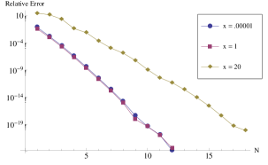
(a) Relative error for PDF of $\chi^{2}$ distribution

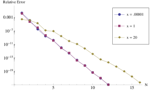
(b) Relative error for CDF of $\chi^{2}$ distribution

Figure 2: Plot of relative error of our method versus the truncation level $N$ for the PDF and CDF of the $\chi^{2}$ distribution at three values of $x$.

Chi-squared
$x$	$10^{-5}$	$10^{-1}$	$1$	$10$	$20$	$50$
$f_{\chi^{2}}(x)$	$1.26\times 10^{2}$	1.20	0.242	$8.50\times 10^{-4}$	$4.05\times 10^{-6}$	$7.83\times 10^{-13}$
$N_{6}$	4	4	4	6	9	14
$N_{15}$	8	8	9	12	15	21
$F_{\chi^{2}}(x)$	$2.52\times 10^{-3}$	0.248	0.683	0.998	$1-7.7\times 10^{-6}$	$1-1.54\times 10^{-13}$
$N_{6}$	3	3	3	4	4	1
$N_{15}$	8	8	8	11	11	12
Inverse Gaussian
$x$	$0.01$	$0.02$	$0.1$	$1$	$100$	$1000$
$f_{IG}(x)$	$3.92\times 10^{-9}$	$3.71\times 10^{-4}$	0.732	0.220	$2.81\times 10^{-4}$	$8.92\times 10^{-6}$
$N_{6}$	12	8	6	5	6	6
$N_{15}$	21	17	14	11	10	11
$F_{IG}(x)$	$1.53\times 10^{-12}$	$5.733\times 10^{-7}$	0.025	0.480	0.944	0.982
$N_{6}$	12	9	6	4	4	3
$N_{15}$	21	17	13	10	8	8

Table 1: Using $k_{i}=10i$, this table shows the value of $N$ required to obtain $6$ digits of accuracy ($N_{6}$) and 15 digits of accuracy ($N_{15}$) at the given values of $x$ using polynomial interpolation. Notice that it becomes harder to approximate these functions to a small relative error when they become very small.

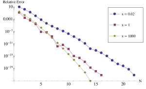
(a) Relative error for PDF of IG distribution.

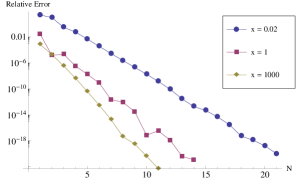
(b) Relative error for CDF of IG distribution

Figure 3: Plot of relative error of our method verses the truncation level $N$ for the PDF and CDF of the IG distribution at three values of $x$.

Results over a range of inputs is shown in Table 1. We show the $x$-values considered as well as the value of $N$ required to obtain a relative precision of $10^{-6}$ and $10^{-15}$. In Figure 2, we also plot the relative error as a function of $N$. Notice that the value of $N$ required is substantially higher when the value of the PDF or CDF takes on very small values, in particular, when $f_{\chi^{2}}(50)\approx 7.83\times 10^{-13}$. This is because $f_{k}(x)$ over approximates $f$ at these points.

The second example we considered is the inverse Gaussian (IG) distribution ([3], Example 1.3.21), for which

$$f_{IG}(x)=\frac{1}{\sqrt{4\pi x^{3}}}e^{-1/(4x)},\quad F_{IG}(x)=1-\mbox{erf}\left(\frac{1}{\sqrt{2x}}\right)$$

$$\psi_{IG}(\lambda)=\tilde{f}_{IG}(\lambda)=e^{-\sqrt{\lambda}}$$

$$\phi_{IG}(\lambda)=-\log\psi_{IG}(\lambda)=\sqrt{\lambda}=\int_{0}^{\infty}(1-e^{-\lambda u})\left[\frac{u^{-3/2}}{2\sqrt{\pi}}\right]du$$

$$\phi^{(n)}_{IG}(\lambda)=\frac{(-1)^{n+1}}{2\sqrt{\pi}}\int_{0}^{\infty}u^{n-3/2}e^{-\lambda u}du=\frac{(-1)^{n+1}}{2\sqrt{\pi}}\Gamma(n-1/2)\lambda^{1/2-n}=\frac{(-1)^{n+1}(2n-3)!}{2^{2(n-1)}(n-2)!}\lambda^{1/2-n}$$

Table 1 also shows the values of $x$ considered, the value of $f_{IG}(x)$, and the value of $N$ needed to obtain relative errors of $10^{-6}$ and $10^{-15}$. Figure 3 shows how the relative error behaves as a function of $N$ for three values of $x$. Similarly to the $\chi^{2}$ distribution, $N$ is largest when the value of the PDF is very close to $0$.

5 Applications to ID distributions which are not known in closed form

We will now consider examples of non-negative ID distributions for which the PDF and CDF are not known in closed form. We will compute them numerically using our method. The resulting plots of the PDFs and CDFs are obtained using MATLAB. Each plot was generated in about 1 second. In order to apply our method, we much first write the Laplace transform in LK form, and then find $\phi(\lambda)$ and the derivatives $\phi^{(n)}(\lambda)$ by computing the integrals in (11). In almost every case below, these integrals can be given in “closed form”, which is to say they can at least be written in terms of special functions for which there are efficient methods for computation. We will assume through out that the drift $a=0$ in (2).

The following special functions will appear throughout this section, we provide their definitions here for convenience:

Gamma function $$\Gamma(a)=\int_{0}^{\infty}z^{a-1}e^{-z}dz,\quad a\neq 0,-1,-2,\dots$$

Lower incomplete gamma function $$\gamma(a,b)=\int_{0}^{b}z^{a-1}e^{-z}dz,\quad b\geq 0,\ a\neq 0,-1,-2,\dots$$

Upper incomplete gamma function $$\Gamma(a,b)=\int_{b}^{\infty}z^{a-1}e^{-z}dz,\quad b>0,\ a\in\mathbb{R}$$

Entire exponential integral $$\mathrm{Ein}(a)=\int_{0}^{a}\frac{1-e^{-z}}{z}dz,\quad a\in\mathbb{R}$$

Dilogatithm $$L_{2}(a)=\int_{1}^{a}\frac{\log(z)}{z-1}dz,\quad a>0$$

See [15], chapters 25, 37, 43 and 45 for more discussion of these functions and methods for efficient computation. For an integer $n\geq 1$, we have $\Gamma(n)=(n-1)!$ and

$$\gamma(n,b)=(n-1)!\left(1-e^{-b}\sum_{m=0}^{n-1}\frac{b^{m}}{m!}\right),$$ (21)

see [9], Equation 3.351.1.

5.1 Right-skewed stable distributions

Here we consider the class of examples with Laplace exponent given by

$$\phi(\lambda)=\int_{0}^{1}\lambda^{\beta}p(d\beta)=\int_{0}^{\infty}(1-e^{-\lambda u})\left[\int_{0}^{1}\frac{u^{-\beta-1}}{\Gamma(-\beta)}p(d\beta)\right]du,$$ (22)

where $p$ is a measure supported on $(0,1)$. The Lévy measure $\Pi$ has a density is given by

$$\Pi^{\prime}(u)=\int_{0}^{1}\frac{u^{-\beta-1}}{\Gamma(-\beta)}p(d\beta).$$

Mixtures of this form are considered in [13] and [12], in which these distributions are used in models of anomalous diffusion.

The Laplace exponent is expressed in (22) and the derivatives $\phi^{(n)}$ for $n\geq 1$ can be computed by using (11), a change in the order of integration, and the definition of the gamma function:

$$\phi^{(n)}(\lambda)=(-1)^{n+1}\int_{0}^{\infty}u^{n}e^{-\lambda u}\left(\int_{0}^{1}\frac{u^{-\beta-1}}{\Gamma(-\beta)}p(d\beta)\right)du=(-1)^{n+1}\int_{0}^{1}\frac{\lambda^{\beta-n}\Gamma(n-\beta)}{\Gamma(-\beta)}p(d\beta)\quad n\geq 1.$$

Since $n$ takes only integer values, $\Gamma(n-\beta)=\Gamma(-\beta)\prod_{m=0}^{n-1}(m-\beta)$, and so the above can be simplified further as

$$\phi^{(n)}(\lambda)=(-1)^{n+1}\int_{0}^{1}\frac{\lambda^{\beta-n}\Gamma(n-\beta)}{\Gamma(-\beta)}p(d\beta) = (-1)^{n+1}\int_{0}^{1}\lambda^{\beta-n}\prod_{m=0}^{n-1}(m-\beta)p(d\beta)$$ (23)

$$= -\frac{1}{\lambda^{n}}\sum_{m=1}^{n}S_{n}^{(m)}\int_{0}^{1}\beta^{m}\lambda^{\beta}p(d\beta)$$

$$= -\frac{1}{\lambda^{n}}\sum_{m=1}^{n}c_{m}(\lambda)S_{n}^{(m)}$$

where $c_{m}(\lambda)=\int_{0}^{1}\beta^{m}\lambda^{\beta}p(d\beta)$ and $\{S_{n}^{(m)}\}$, $n\geq 0$, $0\leq m\leq n$ are the Stirling numbers of the first kind ([15], page 162). These are such that $\prod_{m=0}^{n-1}(\beta-m)=\sum_{m=1}^{n}S_{n}^{(m)}\beta^{m}$, and can computed with a triangular array similarly to Pascal’s triangle using the recursion formula

$$S_{0}^{(0)}=1,\quad S_{n}^{(0)}=0,\quad n\geq 1$$

$$S_{n}^{(m)}=S_{n-1}^{(m-1)}-(n-1)S_{n-1}^{(m)},\quad n,m\geq 1.$$

Let us now consider special cases of $p$ (below, $\delta$ denotes the dirac $\delta$-distribution).

5.1.1 Right-skewed $\alpha$-stable distributions: $\quad p(d\beta)=\delta(\beta-\alpha)d\beta,\quad\ 0<\alpha<1$

Indeed, an important example of this distribution is the right skewed $\alpha$-stable distributions, for which $p$ is a point mass at $\beta=\alpha$, with $0<\alpha<1$ (using Proposition 1.2.11 in [20], this distribution corresponds to the stable distribution $S(\alpha,1,\cos(\pi\alpha/2)^{1/\alpha},0)$). These distributions lie in the family of scaling limits for sums of non-negative i.i.d. random variables with infinite mean. Form (23), $\phi^{(n)}$ can be computed in various ways:

$$\phi^{(n)}(\lambda)=(-1)^{n+1}\frac{\lambda^{\alpha-n}\Gamma(n-\alpha)}{\Gamma(-\alpha)}=-\lambda^{\alpha-n}\prod_{m=0}^{n-1}(\alpha-m)=-\lambda^{\alpha-n}\sum_{m=1}^{n}\alpha^{m}S_{n}^{(m)}$$

The PDFs and CDFs of the right skewed $\alpha$-stable distribution are plotted using our method in Figure 4 for several values of $\alpha$. For example, we compute the PDF of a $(1/2)$-stable distribution at $x=1$ and obtain (in Mathematica)

$$f(1)=0.219695644733861$$

This is exact to 15 decimal places and the computation took approximately half a second. An alternative method for this case is given in [14].

5.1.2 Sums of right-skewed $\alpha$-stable distributions: $\displaystyle\quad p(d\beta)=\sum_{j=1}^{r}d_{j}\delta(\beta-\alpha_{j})d\beta,\ d_{j}\geq 0,\ \displaystyle\ \sum_{j=1}^{r}d_{j}=1$

The previous case can easily be generalized to weighted sums of independent $\alpha$-stable random variables. From (23) it follows that in this case,

$$\phi^{(n)}(\lambda)=(-1)^{n+1}\sum_{j=1}^{r}d_{j}\frac{\lambda^{\alpha_{j}-n}\Gamma(n-\alpha)}{\Gamma(-\alpha_{j})}=-\sum_{j=1}^{r}d_{j}\lambda^{\alpha_{j}-n}\prod_{m=0}^{n-1}(\alpha_{j}-m)=-\sum_{j=1}^{r}d_{j}\lambda^{\alpha_{j}-n}\left(\sum_{m=1}^{n}\alpha_{j}^{m}S_{n}^{(m)}\right).$$

Plot of PDFs of such distributions can be see in Figure 5.

5.1.3 A “uniform mixture” of $\alpha$-stable distributions: $\quad p(d\beta)=d\beta,\ \beta\in(0,1)$

This is an example of a distribution with no finite moments. The Laplace exponent (22) is given by

$$\phi(\lambda)=\int_{0}^{1}\lambda^{\beta}d\beta=\int_{0}^{1}e^{\beta\log\lambda}d\beta=\frac{(\lambda-1)}{\log\lambda}\quad\mbox{if}\ \ \lambda\neq 1,$$

and is $1$ if $\lambda=1$. Higher derivatives of $\phi$ can be computed using (23). The coefficients $c_{m}(\lambda)$, $m=1,2,\dots,n$ can be computed in a few different ways. First, if $\log\lambda\leq 0$, we have

$$c_{m}(\lambda)=\int_{0}^{1}\beta^{m}\lambda^{\beta}d\beta=\int_{0}^{1}\beta^{m}e^{\beta\log\lambda}d\beta=\frac{\gamma(1+m,-\log\lambda)}{(-\log\lambda)^{m+1}}$$ (24)

where $\gamma(a,b)$ is the lower incomplete gamma function (see above). The formula (24) can still be used for $\log\lambda>0$, however this requires analytic continuation of $\gamma$ which is not always easy to compute.

As another approach, we compute $c_{m}(\lambda)$ by treating the cases $|\log\lambda|<1$ and $\geq 1$ separately. If $|\log\lambda|<1$ notice that

$$c_{m}(\lambda)=\int_{0}^{1}\beta^{m}e^{\log(\lambda)\beta}d\beta=\sum_{j=0}^{\infty}(\log\lambda)^{j}\int_{0}^{1}\frac{\beta^{m+j}}{j!}d\beta=\sum_{j=0}^{\infty}\frac{(\log\lambda)^{j}}{(m+j+1)j!}.$$ (25)

If $|\log\lambda|<1$, taking the first 18 terms in this series gives an absolute error of $<10^{-15}$. For $|\log\lambda|\geq 1$, the $c_{m}$’s can be computed recursively by applying integration by parts:

$$c_{0}(\lambda) = \int_{0}^{1}e^{\log(\lambda)\beta}d\beta=\frac{\lambda-1}{\log(\lambda)}$$

$$c_{m}(\lambda) = \int_{0}^{1}\beta^{m}e^{\log(\lambda)\beta}d\beta=\displaystyle\frac{\lambda-mc_{m-1}(\lambda)}{\log(\lambda)},\quad m=1,\dots,n.$$

Since this procedure involves a division by $\log\lambda$, it should only be used when $|\log\lambda|\geq 1$.

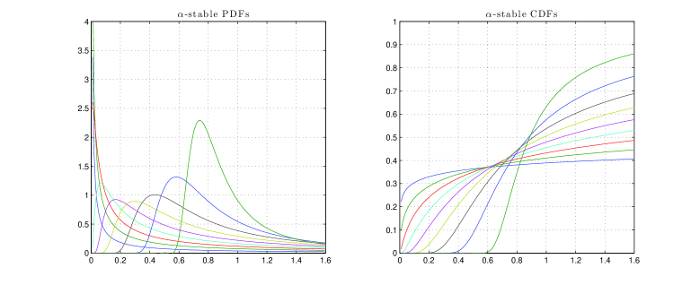
Figure 4: $\alpha$-stable PDFs (left) and CDFs (right) for $\alpha=i/10$ for $i=1,2,\dots,9$. The PDF for $\alpha=0.9$ corresponds to the right-most peak, and $\alpha=.1$ corresponds to the left-most peak (which isn’t visible). The CDF with the steepest slope around $x=0.8$ corresponds to $\alpha=0.9$.

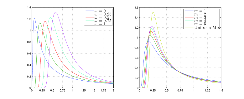
Figure 5: (Left figure) This is the plot of the PDF corresponding to the choice $p_{\omega}(du)=(1-\omega)\delta(x-0.4)+\omega\delta(x-0.8)$ for various choices of $0\leq\omega\leq 1$. By increasing $\omega$, the PDF for $\alpha=0.4$ (on the left) is morphing into the PDF for $\alpha=0.8$ (on the right). (Right figure) These are PDFs corresponding to the sums $p_{m}(du)=\frac{1}{m}\sum_{i=1}^{m}\delta(x-\frac{i}{m+1})$ for $m=1,2,\dots,5$ together with the uniform continuous mixture on $(0,1)$, which has the highest peak.

5.2 Integrals of non-random functions with respect to a Poisson random measure

In this section we consider the large class of non-negative ID distributions which can be expressed in terms of a Poisson stochastic integral of a non random kernel. For a recent review of these integrals, see [16].

Let $(\Omega,{\cal F})$ be a probability space let ${\cal B}$ denote the Borel sigma field on $\mathbb{R}^{n}$. Let $N(\cdot)$ denote a independently scattered Poisson random measure with control measure $\mu$, that is, $\mu$ is a measure on ${\cal B}$ and $N$ is a function $\Omega\times{\cal B}\rightarrow\mathbb{Z}^{+}\cup\{0\}$ such that

• $N(A)\perp N(B)$ if $A,B\in{\cal B}$ are disjoint.

• $\displaystyle N(\bigcup_{m=1}^{n}A_{i})=\sum_{m=1}^{n}N(A_{i})$ if $A_{i}$ are disjoint.

• For each $A\in{\cal B}$, $N(A)$ has a Poisson distribution with mean $\mu(A)$.

Given such a pair $(N,\mu)$ one can define the following stochastic integral

$$I(g)=\int_{\mathbb{R}^{n}}g(\mbox{\boldmath$x$})N(d\mbox{\boldmath$x$})$$ (26)

for a function $g$ on $\mathbb{R}^{n}$, for which $\int_{\mathbb{R}^{n}}\min(1,g(\mbox{\boldmath$x$}))\mu(d\mbox{\boldmath$x$})<\infty$ and, for our purposes, is non-negative. In this case, the random variable $I(g)$ is also non-negative and has Laplace transform

$$\mathbb{E}e^{-\lambda I(g)}=\exp\left(-\int_{\mathbb{R}^{n}}(1-e^{-\lambda g(\mathbf{s})})\mu(d\mathbf{s})\right),\quad\lambda>0.$$ (27)

In order to compute the PDF and CDF of $I(g)$ using our method, (27) must first be rewritten in LK form. In many cases, this can be done with some suitable change of variables $\mathbf{u}=\Phi(\mathbf{s})$ satisfying $u_{1}=(\Phi(\mathbf{s}))_{1}=g(\mathbf{s})$. In this case, (27) becomes

$$\mathbb{E}e^{-\lambda I(g)}=\exp\left(-\int_{0}^{\infty}(1-e^{-\lambda u_{1}})\Pi_{g}(du_{1})\right)$$ (28)

where for any Borel set $A\subset\mathbb{R}^{+}$, the Lévy measure $\Pi_{g}(A)$ can be expressed formally as

$$\Pi_{g}(A)=\int_{A\cap\mathbb{R}^{n-1}}|J(u_{1},u_{2},\dots,u_{n})|(\mu\circ\Phi^{-1})(du_{1},du_{2},\dots,du_{n}),$$ (29)

where $|J|$ is the Jacobian $\partial\Phi^{-1}(u_{1},\dots,u_{n})/\partial(u_{1},\dots,u_{n})$.

To illustrate this, let us now focus on special cases, in dimensions $n=1$ and $n=2$, where this change of variables can be made and our method applied.

5.2.1 One dimensional Poisson integral

Assume $n=1$ and that the integrand $g$ is a monotone, non-negative function with inverse $g^{-1}$. In this case, (27) can be rewritten in LK form using the change of variables $u=g(s)$:

$$\mathbb{E}e^{-\lambda I(g)}=\exp\left(-\int_{0}^{\infty}(1-e^{-\lambda u})\Pi_{g}(du)\right).$$

Since $u=g^{-1}(g(u))$, we get $1=(g^{\prime}\circ g^{-1})(u)\ (g^{-1})^{\prime}(u)$ and hence,

$$\Pi_{g}(du)=\frac{\mbox{\boldmath$1$}_{g((0,\infty))}(u)}{|(g^{\prime}\circ g^{-1})(u)|}(\mu\circ g^{-1})(du)),$$ (30)

where $g((0,\infty))$ denotes the image of $(0,\infty)$ under $g$. Suppose that we want to get the PDF and CDF of

$$I(g)=\int_{0}^{\infty}e^{-s/\eta}N(ds)$$

where $g(s)=e^{-s/\eta}$, $\eta>0$ is a parameter and the control measure $\mu$ is Lebesgue. In this case, a simple calculation shows that (30) becomes

$$\Pi_{g}(du)=\left(\frac{\eta}{u}\right)\mbox{\boldmath$1$}_{(0,1]}(u)du.$$

Thus, for this example,

$$\phi(\lambda)=\int_{0}^{1}(1-e^{-\lambda u})\left(\frac{\eta}{u}\right)du=\eta\mathrm{Ein}(\lambda),$$

where $\mathrm{Ein}(\lambda)$ is the entire exponential integral defined earlier. The derivatives $\phi^{(n)}(\lambda)$, for $n\geq 1$ can be given in closed form

$$\phi^{(n)}(\lambda)=(-1)^{n+1}\eta\int_{0}^{1}u^{n-1}e^{-\lambda u}du=\frac{(-1)^{n+1}\eta}{\lambda^{n}}\gamma(n,\lambda)=\frac{(-1)^{n+1}\eta}{\lambda^{n}}\left((n-1)!-e^{-\lambda}\sum_{m=0}^{n-1}\frac{(n-1)!}{m!}\lambda^{m}\right),$$

where the last equality follows from (21). We’ve plotted the PDF and CDF of the random variable $I(e^{-s/\eta})$ for various values of $\eta$ in Figure (6) using our method. Note that since the range of integration here is $(0,\infty)$, the method described in [24] doesn’t readily apply.

Figure 6: Plots of the PDF and CDF for the Poisson stochastic integral $I(e^{-s/\eta})$ with various values of the parameter $\eta$, which plays the role of a shape parameter. The PDF for $\eta=0.5$ is the highest on the left.

5.2.2 Integration with respect to non-negative Lévy process with a non-negative kernel

In this example, we generalize the previous case by looking at integration with respect to a non-negative Lévy process, or equivalently, a one-dimensional non-negative ID random measure $L$ with control measure $\mu$. $L$ is a random measure which satisfies the same conditions as the Poisson random measure $N$, except condition $(\mathrm{iii})$ is replaced by

• There exists a Lévy measure $\Pi$ such that for any $A\in{\cal B}$, the distribution of $L(A)$ has Laplace transform

  $$\mathbb{E}e^{-\lambda L(A)}=\exp\left(-\mu(A)\int_{0}^{\infty}(1-e^{-\lambda u})\Pi(du)\right).$$

Notice that the Poisson random measure $N$ corresponds to the choice $\Pi(du)=\delta(u-1)du$. For a given function $g$, the stochastic integral $I_{L}(g)$ can be defined in terms of a two-dimensional Poisson stochastic integral:

$$I_{L}(g)=\int_{0}^{\infty}g(s)L(ds)\equiv\int_{0}^{\infty}\int_{0}^{\infty}ug(z)N(du,dz),$$ (31)

where the control measure of $N$ is given now by $\Pi(du)\mu(dz)$. Observe that the kernel $g$ must now satisfy $\int_{0}^{\infty}\int_{0}^{\infty}\min(1,ug(z))\Pi(du)\mu(dz)<\infty$

Assume now for simplicity that $\Pi(du)=\Pi(u)du$ for some function $\Pi$ and that $g$ is a non-negative monotone function with inverse $g^{-1}$. In this case, we can obtain the LK form corresponding to $I_{L}$:

$$\mathbb{E}e^{-\lambda I_{L}(g)} = \exp\left(-\int_{0}^{\infty}\int_{0}^{\infty}(1-e^{-\lambda ug(z)})\Pi^{\prime}(u)du\mu(dz)\right)$$

$$= \exp\left(-\int_{0}^{\infty}(1-e^{-\lambda v})\Pi^{\prime}_{g}(v)dv\right)$$

where we have made the change of variables $v=ug(z)$, $z^{\prime}=z$ and the measure $\Pi_{g}(dv)$ is given by

$$\Pi^{\prime}_{g}(v)=\int_{0}^{\infty}\Pi^{\prime}\left(\frac{v}{g(z^{\prime})}\right)\frac{1}{g(z^{\prime})}\mu(dz^{\prime}).$$ (32)

To demonstrate our method in this case, consider

$$I_{L}(g)=\int_{0}^{\infty}e^{-z/\eta}L(dz)=\int_{0}^{\infty}\int_{0}^{\infty}ue^{-z/\eta}N(du,dz)$$

where $g(z)=e^{-z/\eta}$ with $\eta>0$, $\mu$ Lebesgue, and $\Pi(du)=\kappa u^{-1}e^{-u/\theta}du$, which is the Lévy measure corresponding to the Gamma distribution with shape $\kappa>0$ and scale $\theta>0$ ([3], Example 1.3.22). With the change of variables $w=ue^{z/\eta}$, (32) implies

$$\Pi^{\prime}_{g}(u)=\int_{0}^{\infty}\Pi^{\prime}\left(ue^{z/\eta}\right)e^{z/\eta}dz=\frac{\eta\kappa}{u}\int_{u}^{\infty}w^{-1}e^{-w/\theta}dw=\frac{\eta\kappa}{u}\Gamma\left(0,\frac{u}{\theta}\right)$$

We can now compute the corresponding Laplace exponent for this case:

$$\phi(\lambda)=\int_{0}^{\infty}(1-e^{-\lambda u})\Pi^{\prime}_{g}(u)du =\eta\kappa\int_{0}^{\infty}\frac{(1-e^{\lambda u})}{u}\Gamma\left(0,\frac{u}{\theta}\right)du$$

$$=\eta\kappa\int_{0}^{\infty}\int_{0}^{\lambda}e^{-ut}\int_{u}^{\infty}\left(w^{-1}e^{-w/\theta}\right)dw\ dt\ du$$

$$=\eta\kappa\int_{0}^{\lambda}\left[\int_{0}^{\infty}\int_{0}^{w}(w^{-1}e^{-ut-w/\theta})du\ dw\right]dt$$

$$=\eta\kappa\int_{0}^{\lambda}\frac{1}{t}\left[\int_{0}^{\infty}w^{-1}e^{-w/\theta}(1-e^{-wt})dw\right]dt$$ (33)

$$=\eta\kappa\int_{0}^{\lambda}\frac{1}{t}\int_{0}^{\infty}\left(e^{-w/\theta}\int_{0}^{t}e^{-ws}ds\right)dwdt$$

$$=\eta\kappa\int_{0}^{\lambda}\frac{1}{t}\left[\int_{0}^{t}\int_{0}^{\infty}e^{-w(s+1/\theta)}dw\ ds\right]dt$$

$$=\eta\kappa\int_{0}^{\lambda}\frac{\log(1+t\theta)}{t}dt=\eta\kappa L_{2}(1+\lambda\theta)$$ (34)

The derivatives of $\phi$ can also be computed exactly in this case. Using (11) and (21),

$$\phi^{(n)}(\lambda) =(-1)^{n+1}\eta\kappa\int_{0}^{\infty}u^{n-1}e^{-\lambda u}\Gamma\left(0,\frac{u}{\theta}\right)du$$

$$=(-1)^{n+1}\eta\kappa\int_{0}^{\infty}u^{n-1}e^{-\lambda u}\int_{u}^{\infty}(w^{-1}e^{-w/\theta})dwdu$$

$$=(-1)^{n+1}\eta\kappa\int_{0}^{\infty}w^{-1}e^{-w/\theta}\left[\int_{0}^{w}u^{n-1}e^{-\lambda u}du\right]dw$$

$$=(-1)^{n+1}\eta\kappa\int_{0}^{\infty}w^{-1}e^{-w/\theta}\left[\frac{(n-1)!}{\lambda^{n}}-e^{-w\lambda}\sum_{m=0}^{n-1}\frac{(n-1)!}{m!}\frac{w^{m}}{\lambda^{n-m}}\right]dw$$

$$=(-1)^{n+1}\eta\kappa\frac{(n-1)!}{\lambda^{n}}\left[\int_{0}^{\infty}w^{-1}e^{-w/\theta}(1-e^{-w/\theta})dw-\sum_{m=1}^{n-1}\frac{\lambda^{m}}{m!}\int_{0}^{\infty}w^{m-1}e^{-w(\lambda+1/\theta)}dw\right]$$

$$=(-1)^{n+1}\eta\kappa\frac{(n-1)!}{\lambda^{n}}\left[\log(1+\lambda\theta)-\sum_{m=1}^{n-1}\frac{(\lambda\theta)^{m}}{m\ (1+\lambda\theta)^{m}}\right],$$

where the first integral in the second to last line above is computed as in (33). Alternatively, $\phi^{(n)}(\lambda)$ above can also be given simply in terms of the Gauss hypergeometric function $\ {}_{2}F_{1}(\alpha,\beta,\gamma,x)$ ([9], Equation 6.455.1, page 657)

$$\phi^{(n)}(\lambda)=(-1)^{n+1}\eta\kappa\frac{\theta^{n}(n-1)!}{n}\ _{2}F_{1}(n,n,n+1,\lambda\theta).$$

In Figure 7 we’ve plotted the PDF and CDF of (31) for $\theta=1$ and various values of the product $\rho=\eta\kappa$ using our method.

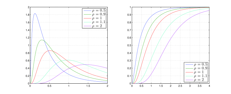
Figure 7: Plots of the PDF and CDF for the Poisson stochastic integral $I_{L}(e^{-s/\eta})$ with various values of the parameter $\eta$.

6 Guide to software

In this section, we will explain how to use the software written to implement the method discussed in this paper. Versions of this code exist in MATLAB and Mathematica, and are freely available by request form the authors. Each version will include a file containing examples to assist in using the code.

To begin using the code, download the file NNINFDIV.zip and extract the directory NNINFDIV. This directory contains both the MATLAB and Mathematica programs in separate folders. We will now focus on these separately.

6.1 MATLAB version

To use the MATLAB version, launch MATLAB and add the directory NNINFDIV/MATLAB to MATLAB’s default path by typing

$\gg$ path(path,‘mypath/NNINFDIV/MATLAB’)

where ‘mypath’ is the path which leads to the directory NNINFDIV. You are now ready to use the code provided in this package.

The main function is called nninfdiv. This function takes in 5 arguments in the following order:

X Scalar or vector of input values. Must be positive.

DIST A cell array which specifies the distribution and parameters (see below)

FUNC Type of function: ‘pdf’ or ‘cdf’

METHOD Extrapolation method: ‘polynomial’ or ‘rational’

TOL Target relative error tolerance

The last three inputs FUNC,METHOD and TOL are optional, and take default values ’pdf’, ’polynomial’ and $10^{-6}$. The input DIST is a cell array which contains the name of the desired distribution followed by the parameters. Possibilities for DIST are

{’chi-squared’,df,1} Chi-squared distribution with df degrees of freedom.

{’chi-squared’,df,[c1,...,cn]} Weighted sum of chi-squared distributions

{’alpha stable’,a,c} $$\mbox{Alpha-stable distribution with $\alpha$ = a and scaling $c$}.$$

{’alpha stable’,[a1,...,an],[c1,...,cn]} $$\mbox{Sum of $n$ weighted alpha-stable distributions}.$$

{’uniform mix’} Uniform mix from Section 5.1.3.

{’ou poisson’,eta} The integral $$I(e^{-s/\eta})$$ from Section 5.2.1

{’ou gamma’,eta,kappa} $$\mbox{The integral $I_{L}(e^{-s/\eta})$ from Section \ref{s:ougamma}}.$$

The scaling constants seen in the alpha-stable and chi-squared examples above compute the PDF/CDF of the scaled random variables $cX$ for $c>0$ in the single alpha-stable and single chi-squared case. Likewise, in the weighted case, they return the PDF/CDF of $c_{1}X_{1}+c_{2}X_{2}+\dots c_{n}X_{n}$ with $c_{i}>0$, and $X_{i}$ is chi-squared with df degrees of freedom or is alpha-stable with $\alpha=$ai.

Since the input for nninfdiv is long, it is often useful to define a function handle in order to call the function more easily. For example, consider the $\alpha$-stable distribution with $\alpha=2/3$. We define the PDF of this distribution in the variable f by typing

$\gg$ f = @(x) nninfdiv(x,{’alpha stable’,2/3,1},’pdf’,’polynomial’,1e-6);

The function f now computes the PDF of the alpha-stable distribution with $\alpha=2/3$ to within a relative error of $10^{-6}$ using the polynomial interpolation method. For example, you may now type

$$\gg\texttt{f(1)} x=1$$ Computes the PDF at

$$\gg\texttt{f([1 2 3])} x=1,2 3$$ Computes the PDF at and .

$$\gg\texttt{plot([.05:.05:2],f([.05:.05:2]))}$$ Plots the PDF on the interval (0,2]

Remark: Obtaining relative errors less than $10^{-6}$ is sometimes difficult. If your error tolerance cannot be reached, the program will return the best estimate possible in double precision. If high precision is preferred over speed, the Mathematica version should be used.

6.2 Mathematica version

To use the Mathematica version, launch Mathematica open the file NNINFDIV.nb located in the directory NNINFDIV/Mathematica. Once this file is open, select all its contents by pressing alt-a on a PC or cmd-a on a Mac. Then compile the code by pressing shift-return. You are now ready to use the code in a separate notebook.

The main program is called NNInfDiv (capitalization matters). This program is called with 4 arguments:

X Input value. Must be a positive scalar.

DIST A list which specifies the distribution and parameters (see below)

FUNC Type of function: ”PDF” or ”CDF”

TOL Relative error tolerance

The last two inputs FUNC and TOL are optional, taking default values “PDF” and $10^{-15}$ respectively. Possibilities for DIST include

{"Chi-Squared",{c1,..cn}} Sum of weighted chi-squared with weights c1,...,cn.

{"Alpha Stable",a,c} $$\mbox{Alpha-stable distribution with $\alpha$ = {a} and scaling {c}}.$$

{"Uniform Mix"} Uniform mix from Section 5.1.3.

{"OU Poisson",eta} The integral $$I(e^{-s/\eta})$$ from Section 5.2.1

{"OU Gamma",eta,kappa} $$\mbox{The integral $I_{L}(e^{-s/\eta})$ from Section \ref{s:ougamma}}.$$

The scaling constants seen in the chi-squared and alpha-stable cases above refer to the random variables $cX$ with $c>0$ in the alpha-stable case and $c_{1}X_{1}+\dots c_{n}X_{n}$ in the chi-squared case, with $X_{i}$ i.i.d chi-squared.

To simplify the call to this function, one can make a user defined function. For example, to make a function F which computes the CDF of an $\alpha$-stable distribution with $\alpha=2/3$, one can type

F[x_] := NNInfDiv[x,{ "Alpha Stable" , 2/3 , 1 } , "CDF" ]

The function F now computes the CDF of $\alpha$-stable distribution with $\alpha=2/3$ to a relative precision of $10^{-15}$. For example, one can now enter

F[1] Computes the CDF at $$x=1$$

Table[F[x],{x,{1,2,3}}] Computes the CDF at $$x=1,2 3$$ and

ListPlot[Table[{x,F[x]},{x,0,2,.05}],Joined -> True] Plots the CDF on the interval [0,2]

Remark: Using NNInfDiv with Mathematica’s Plot function is very slow, which is why we used the ListPlot function above. For faster plotting and function evaluation, the MATLAB version of the code should be used.

Mark Veillette (mveillet@bu.edu) &
Murad Taqqu (murad@math.bu.edu)
Dept. of Mathematics
Boston University
111 Cummington St.
Boston, MA 02215

References

- [1] J. Abate, G. L. Choudhury, and W. Whitt. An introduction to numerical transform inversion and its application to probability models. In W. K. Grassman, editor, Computational Probability, pages 258–322. Kuwer Academic Publishers, USA, 2000.
- [2] Joseph Abate and Ward Whitt. The Fourier-series method for inverting transforms of probability distributions. Queueing Systems Theory Appl., 10(1-2):5–87, 1992.
- [3] D. Applebaum. Lévy Processes and Stochastic Calculus. Cambridge University Press, Cambridge, UK, 2004.
- [4] J. Bertoin. Lévy Processes. Cambridge University Press, Cambridge, UK, 1996.
- [5] J. Bertoin. Subordinators: Examples and Applications, in: Lecture Notes in Mathematics, volume 1717. Springer, Berlin, 1999.
- [6] Roland Bulirsch and Josef Stoer. Asymptotic upper and lower bounds for results of extrapolation methods. Numer. Math., 8:93–104, 1966.
- [7] W. Feller. An Introduction to Probability Theory and its Applications, volume 2. John Wiley and Sons, Inc, New York, second edition, 1971.
- [8] G. A. Frolov and M. Y. Kitaev. Improvement of accuracy in numerical methods for inverting Laplace transforms based on the Post-Widder formula. Computers and Mathematics with Applications, 36(5):23–34, 1998.
- [9] I. S. Gradshteyn and I. M. Ryzhik. Table of integrals, series, and products. Elsevier/Academic Press, Amsterdam, seventh edition, 2007. Translated from the Russian, Translation edited and with a preface by Alan Jeffrey and Daniel Zwillinger, With one CD-ROM (Windows, Macintosh and UNIX).
- [10] D. L. Jagerman. An inversion technique for the Laplace transform. Bell System Tech. J., 61(8):1995–2002, 1982.
- [11] D. C. Joyce. Survey of extrapolation processes in numerical analysis. SIAM Rev., 13:435–490, 1971.
- [12] M. Kovacs and M. Meerschaert. Ultrafast subordinators and their hitting times. Publications de L’Institut Mathematique, 94(71):193–206, 2006.
- [13] M. Meerschaert and H. Scheffler. Stochastic model for ultraslow diffusion. Stochastic Processes and their Applications, 116(9):1213–1235, 2006.
- [14] John P. Nolan. Numerical calculation of stable densities and distribution functions. Comm. Statist. Stochastic Models, 13(4):759–774, 1997. Heavy tails and highly volatile phenomena.
- [15] Keith Oldham, Jan Myland, and Jerome Spanier. An atlas of functions. Springer, New York, second edition, 2009. With Equator, the atlas function calculator, With 1 CD-ROM (Windows).
- [16] G. Peccati and M. S. Taqqu. Wiener Chaos: Moments, Cumulants and Diagrams. Bocconi Press and Springer Verlag, 2010. To appear.
- [17] J. Pitman. Combinatorial stochastic processes, volume 1875 of Lecture Notes in Mathematics. Springer-Verlag, Berlin, 2006. Lectures from the 32nd Summer School on Probability Theory held in Saint-Flour, July 7–24, 2002, With a foreword by Jean Picard.
- [18] John Riordan. An introduction to combinatorial analysis. Dover Publications Inc., Mineola, NY, 2002. Reprint of the 1958 original [Wiley, New York; MR0096594 (20 #3077)].
- [19] Steven Roman. The umbral calculus, volume 111 of Pure and Applied Mathematics. Academic Press Inc. [Harcourt Brace Jovanovich Publishers], New York, 1984.
- [20] Gennady Samorodnitsky and Murad S. Taqqu. Stable non-Gaussian random processes. Stochastic Modeling. Chapman & Hall, New York, 1994. Stochastic models with infinite variance.
- [21] Ken-iti Sato. Lévy processes and infinitely divisible distributions, volume 68 of Cambridge Studies in Advanced Mathematics. Cambridge University Press, Cambridge, 1999. Translated from the 1990 Japanese original, Revised by the author.
- [22] Fred W. Steutel and Klaas van Harn. Infinite divisibility of probability distributions on the real line, volume 259 of Monographs and Textbooks in Pure and Applied Mathematics. Marcel Dekker Inc., New York, 2004.
- [23] M Veillette and M. S. Taqqu. Numerical computation of first-passage times of increasing Lévy processes. Methodology and Computing in Applied Probability, 2009.
- [24] Mark Veillette and Murad Taqqu. Distribution functions of Poisson random integrals: Analysis and computation, 2010. Preprint: http://arxiv.org/abs/1004.5338