Theoretical Analysis of Drag Resistance
in Amorphous Thin Films Exhibiting Superconductor-Insulator-Transition

Abstract

The magnetical field tuned superconductor-insulator transition in amorphous thin films, e.g., Ta and InO, exhibits a range of yet unexplained curious phenomena, such as a putative low-resistance metallic phase intervening the superconducting and the insulating phase, and a huge peak in the magnetoresistance at large magnetic field. Qualitatively, the phenomena can be explained equally well within several significantly different pictures, particularly the condensation of quantum vortex liquid, and the percolation of superconducting islands embedded in normal region. Recently, we proposed and analyzed a new measurement in Ref. Zou et al., 2009 that should be able to decisively point to the correct picture: a drag resistance measurement in an amorphous thin-film bilayer setup. Neglecting interlayer tunneling, we found that the drag resistance within the vortex paradigm has opposite sign and is orders of magnitude larger than that in competing paradigms. For example, two identical films as in Ref. Sambandamurthy et al., 2004 with $25$nm layer separation at $0.07$K would produce a drag resistance $\sim 10^{-4}\Omega$ according the vortex theory, but only $\sim 10^{-12}\Omega$ for the percolation theory. We provide details of our theoretical analysis of the drag resistance within both paradigms, and report some new results as well.

I Introduction

Amorphous thin film superconductors exhibit a variety of fascinating quantum phenomena, due to the importance of fluctuation and disorder in two dimensions. Early theoreticalFisher and Lee (1989); Fisher (1990); Wen and Zee (1990); Fisher et al. (1990); Cha et al. (1991); Wallin et al. (1994) and experimentalHaviland et al. (1989); Hebard and Paalanen (1990); Paalanen et al. (1992); Valles et al. (1992); Liu et al. (1993); Hsu et al. (1995); Valles et al. (1994); Yazdani and Kapitulnik (1995); Hsu et al. (1998); Goldman and Markovic (1998) work focus on the quantum superconductor-insulator-transition (SIT) in these materials. As one increases the perpendicular magnetic field or decreases the film thickness, the film changes from superconducting to insulating. An appealing theoretical picture of the SIT is that the amplitude of the superconducting order parameter remains finite across the transition, and the transition is driven by phase fluctuations, which can be viewed as the condensation of vortices. Therefore the insulator is described as a vortex superfluid, and the transition point is nearly self dual: it could be described either as the condensation of Cooper pairs, or of vortices. This Cooper-pair - vortex duality also suggests that the critical resistance at the transition should be $R_{\square}=h/4e^{2}=6.5k\Omega$, which is consistent with observations on strongly disordered samples Steiner et al. . A variety of other experiments shows a transition with a critical resistance of the same order as $R_{Q}=h/4e^{2}$.

In recent years, experiments on these amorphous thin films have revealed more surprising results, mainly in transitions tuned by normal magnetic field. One of these raises the possibility that a metallic phase intervenes between the superconducting and the insulating phasesEphron et al. (1996); Mason and Kapitulnik (1999, 2001); Sambandamurthy et al. (2004); Steiner and Kapitulnik (2005); Seo et al. (2006); Qin et al. (2006); Li et al. (2010). Near the ”SIT critical point”, as temperature is lowered below $\sim 100$mK, the resistance curve starts to level off, indicating the existence of a novel metallic phase, with a distinct nonlinear $I-V$ characteristics at least in Ta films that are interpreted as a consequence of vortex dynamics Seo et al. (2006). Another interesting experimental finding is the nonmonotonic behavior of the magnetoresistanceSambandamurthy et al. (2004); Baturina et al. (2004); Steiner and Kapitulnik (2005); Gantmakher and Dolgopolov (2010). As one increases magnetic field further from the ”SIT point”, the resistance climbs up quickly to very large value in InO and TiN films, before it plummeting back to the normal state resistance, as shown in FIG. 1. In Ta and MoGe films, as well as some InO films, the resistance peak is not as large, but is still apparent Ephron et al. (1996); Mason and Kapitulnik (1999, 2001); Steiner and Kapitulnik (2005); Seo et al. (2006); Qin et al. (2006).

Figure 1: A typical magnetoresistance curve of amorphous thin film superconductors. As the magnetic field $B$ increases, the superconducting phase is destroyed, and a possible metallic phase emerges. After which the system enters an insulating phase, where the magnetoresistance reaches its peak. The resistance drops down and approaches normal state value as $B$ is further increased.

Two competing paradigms may account for these phenomena. On the one hand, within the quantum vortex pictures Fisher (1990); Feigelman et al. (1993); Balents and Fisher (2005); Galitski et al. (2005), the insulating phase at the peak of the magnetoresistance implies the condensation of quantum vortices, and the high field negative magnetoresistance indicates the gradual depairing of Cooper pairs and the appearance of a finite electronic density of states at the Fermi level. The intervening metallic phase is described as a delocalzed but yet uncondensed diffusive vortex liquid as described in Ref. Galitski et al., 2005. In this picture disorder and charging effects are most important on length scales smaller or of order $\xi$ (the superconducting coherence length, typically of order $10nm$). On the other hand, the percolation paradigmShimshoni et al. (1998); Ghosal et al. (2001); Dubi et al. (2006, 2007); Spivak et al. (2008) describes the amorphous film as a mixture of superconductor and normal or insulating puddles, with disorder playing a role at scales larger than $\xi$. Particularly germane is the picture in Ref. Dubi et al., 2007 which phenomenologically captures both a metallic phase as well as the strongly insulating phase by assuming superconducting islands exhibit a Coulomb blockade for electrons. This way the peak in the magnetoresistance arises from electron transport though the percolating normal regions consisting of narrow conduction channels. Yet a third theory tries to account for the low field superconductor-metal transition using a phase glass model Dalidovich and Phillips (2002); Wu and Phillips (2006) (see, however, Ref. Ikeda, 2007 which argues against these results), but does not address the full magnetoresistance curve. Qualitatively, both paradigms above are consistent with magnetoresistance observations, and recent tilted fieldJohansson et al. , AC conductanceCrane et al. (2007), Nernst effectSpathis et al. (2008), and Scanning Tunneling SpectroscopicSacepe et al. (2008) measurements cannot distinguish between them. Particularly intriguing is the origin of the metallic phase - is it vortex driven or does it occur due to electronic conduction channels dominating transport through the film?

Figure 2: Our proposed bilayer setup for the drag resistance measurement. A current bias $I_{1}$ is applied in one layer, and a voltage $V_{2}$ is measured in the other layer. The drag resistance $R_{D}$ is defined as $R_{D}=V_{2}/I_{1}$.

Given the similarity in the predictions of the distinct vortex-condensation and percolation paradigms, an experiment that distinguishes between them would be highly desirable. We propose that a thin film ”Giaever transformer”Giaever (1965) experiment (FIG. 2) can qualitatively distinguish between these two paradigms. The original design of a Giaever transformer consists of two type-II superconductors separated by an insulating layer in perpendicular magnetic fields. A current in one layer moves the vortex lattice in the entire junction, yielding the same DC voltage in both layers. Determining the drag resistance $R_{D}=V_{2}/I_{1}$ in a similar bilayer structure of two amorphous superconducting thin films should qualitatively distinguish between the two paradigms (see also Refs. Michaeli and Finkel’stein, 2006; Mason and Kapitulnik, 2002): within the vortex paradigm, vortices in one layer drag the vortices in the other, but within the percolation picture, the drag resistance is solely due to interlayer ”Coulomb drag”, as studied in semiconductor heterostructures Gramila et al. (1991).

The first qualitative difference between vortex drag and Coulomb drag is the sign of the drag voltage $V_{2}$. Denoting the voltage drop in the driving layer as $V_{1}$, it is easy to see that $V_{1}$ and $V_{2}$ have the same sign if they are produced by vortex motion, because vortices in the two layers move in the same direction transverse to the current bias $I_{1}$. (We note in passing that if the second layer is in a closed circuit, the vortex drag would induce a current in the opposite direction in the secondary layer, since no outside voltage source balances the EMF produced by the vortex motion.) On the other hand, $V_{1}$ and $V_{2}$ would have opposite signs if they are due to electron Coulomb drag, because $V_{2}$ has to balance the drag force to ensure the open circuit condition in the second layer. In other words, Coulomb drag would try to produce current in the same direction in the primary and secondary layer.

More importantly, we have found that in the vortex scenario, the drag resistance is expected to be several orders of magnitude larger than that in other models. Partially this is expected because in these films, the sheet carrier density $\sim 10^{16}$cm^-2 is much larger than the vortex density $\sim B/\Phi_{0}\sim 10^{10}$cm^-2, and the drag effect is typically smaller for larger densities. For example, two identical films as in FIG. 2(b) of Ref. Sambandamurthy et al., 2004 with $25$nm center-to-center layer separation at $0.07$K would produce a drag resistance $\sim 10^{-4}\Omega$ according the vortex theory (see FIG. 3), but only $\sim 10^{-12}\Omega$ for the percolation theory (see FIG. 4). But as we shall show below, the large vortex drag effect is also a consequence of the extremely high magneto-resistance slope, which has different implications for the vortex condensation and percolation pictures. The strength of the thin-film Giaever tranformer experiment would therefore be in the transition region where the metallic phase transforms into the insulating phase, and the magneto-resistance is at a maximum.

We believe that these qualitative differences between the drags in the two paradigms are quite general for each paradigm, and does not depend the various microscopic assumptions made in various flavors of these phenomenological pictures. We will support these claims by analyzing the drag resistance between two identical thin films within a representative theoretical framework in the vortex Galitski et al. (2005) and percolation paradigms Dubi et al. (2006). We will restrict ourselves to the standard drag measuring geometry assuming zero tunneling between the layers. We expect that allowing small tunneling will stregthen the effect; we will pursue this possiblity in future work.

This paper is organized as follows. In Sec. II, we extend the quantum vortex formalism to bilayers, and then we calculate the drag resistance in the insulating and the metallic regime, respectively. The effect of unpaired electrons on the drag resistance is also studied. In Sec. III, we review the percolation theory of Ref. Dubi et al., 2006, and then extend this theory to bilayers as well, in order to calculate the drag resistance. In Sec. IV, we briefly discuss the drag resistance behavior within the phase glass model of Refs. Dalidovich and Phillips, 2002; Wu and Phillips, 2006. Finally, we summarize and discuss our results in Sec.V. Some details are provided in appendices.

II Drag resistance in the quantum vortex paradigm

II.1 The vortex description of double-layer amorphous films

Within the quantum vortex paradigm, the insulating phase has been explained as a superfluid of vortices by the ”dirty boson” model of Ref. Fisher, 1990, while the metallic phase is expected to be an uncondensed vortex liquid (see also Ref. Feigelman et al., 1993). This picture has been pursued by Ref. Galitski et al., 2005 which argues that vortices form a Fermi liquid for a range of magnetic field, thereby explaining the metallic phase. At larger fields, where the insulating phase breaks down, it is claimed that gapless bogolubov quasi particles nicknamed spinons, i.e., unpaired fermions with finite density of states at the Fermi energy, become mobile, impede vortex motions, destroy the insulating phase, and suppress the resistance down to normal metallic values.

We will concentrate on the case where no interlayer Josephson coupling exists, and the vortex drag comes from the magnetic coupling between vortices in different layers which tends to align themselves vertically to minimize the magnetic energy. To calculate the drag resistance in a bilayer setup, it is crucial to derive the vortex interaction potential due to the current-current magnetic coupling between the layers, which is captured by the $B^{2}$ term in the Maxwell action. We achieve this by both a field theory formalism and a classical calculation. The classical calculation is relegated to Appendix C.

Let us next derive the vortex action. Treating the superconducting film as a Cooper pair liquid, we have the following partition function

$$\mathcal{Z}=\int\mathcal{D}\rho_{1}\mathcal{D}\rho_{2}\mathcal{D}\theta_{1}\mathcal{D}\theta_{2}\mathcal{D}\vec{A}e^{-S},$$ (1)

where

$$S = \int_{0}^{\beta}\mathrm{d}\tau\left\{\int\mathrm{d}^{2}r\sum_{n=1,2}\hbar\rho_{n}\partial_{\tau}\theta_{n}+H_{0}+H_{int}\right\},$$

$$H_{0} = \int\mathrm{d}^{2}r\sum_{n=1,2}\frac{\rho_{s}}{2\hbar^{2}}\left(\hbar\nabla\theta_{n}-\frac{2e}{c}\vec{A}_{ext}-\frac{2e}{c}\vec{A}\right)^{2}$$

$$+ \frac{1}{4\pi}\int\mathrm{d}^{3}r\vec{B}^{2},$$

$$H_{int} = \int\mathrm{d}^{2}r\int\mathrm{d}^{2}r^{\prime}\frac{1}{2}\sum_{n=1,2}\rho_{n}(r)V_{i}(r-r^{\prime})\rho_{n}(r^{\prime})$$

$$+ \rho_{1}(r)V_{e}(r-r^{\prime})\rho_{2}(r^{\prime}),$$

where $a$ is the (center-to-center) layer-separation, $\rho_{n}$ and $\theta_{n}$ are the 2d density and phase fluctuation of the $n-$th layer Cooper pair field, respectively, $A$ and $A_{ext}$ are the fluctuating and external part of the electromagnetic field, respectively. The intralayer Coulomb interaction $V_{i}(r)=(2e)^{2}/r$ (whose 2d Fourier transform would be $2\pi(2e)^{2}/q$), and the interlayer Coulomb interaction $V_{e}(r)=(2e)^{2}/\sqrt{r^{2}+a^{2}}$ (whose 2d Fourier transform is $2\pi(2e)^{2}/qe^{-qa}$). $\rho_{s}$ is the superfluid phase stiffness of each layer, which can be determined approximately from the Kosterlitz-Thouless temperature $T_{KT}$:

$$T_{KT}=\frac{\pi}{2}\rho_{s}.$$ (2)

Next, we follow a procedure of vortex-boson duality transformation taking into account the $B^{2}$ term (which will be the origin of the interlayer vortex interaction), and obtain the following dual action for the vortex field $\psi_{vn}$ of the $n$-th layer and two U(1) gauge fields $\alpha_{\mu}$ and $\beta_{\mu}$ (see Appendix B for details):

$$S =\sum_{\vec{q},\omega}\left\{\sum_{n=1,2}\left[-i\hbar\delta\rho_{vn}\omega\phi_{n}+\frac{1}{2}\delta\rho_{vn}U_{i}\delta\rho_{vn}\right.\right.$$

$$+\left.\frac{1}{2m_{v}}\left(\left(\hbar\vec{q}-e_{1}^{*}\frac{\vec{\alpha}}{c^{*}_{1}}+(-1)^{n}e_{2}^{*}\frac{\vec{\beta}}{c^{*}_{2}}\right)\psi_{vn}\right)^{2}\right]$$

$$+\delta\rho_{v1}U_{e}\delta\rho_{v2}+\frac{1}{4\pi}(\omega^{2}-c_{*1}^{2}q^{2})\left(\frac{\vec{\alpha}}{c^{*}_{1}}\right)^{2}$$

$$+\left.\frac{1}{4\pi}(\omega^{2}-c_{*2}^{2}q^{2})\left(\frac{\vec{\beta}}{c^{*}_{2}}\right)^{2}\right\},$$ (3)

where $\delta\rho_{vn}=\rho_{vn}-B/\Phi_{0}$, $\Phi_{0}$ is the flux quantum, $\rho_{vn}=\psi_{vn}^{\dagger}\psi_{vn}$, $\phi_{n}$ is the phase of the vortex field $\psi_{vn}$, and $m_{v}$ is the vortex mass. Since there is still controversy over the theoretical value of $m_{v}$, we chose to determine the vortex mass from experiments. As discussed in Appendix A, for the InO film of Ref. Sambandamurthy et al., 2004, we obtain $m_{v}\approx 19m_{e}$ where $m_{e}$ is the bare electron mass.

$\alpha_{\nu}$ and $\beta_{\nu}$ are gauge fields which mediate the symmetric and antisymmetric part of the vortex-vortex interaction. They are related to the Cooper pair currents $j_{n\mu}$ in the $n-$the layer by

$$j_{1\mu}+j_{2\mu} = \frac{e_{1}^{*}}{\pi\hbar}\epsilon_{\mu\nu\eta}\partial_{\nu}\alpha_{\eta},$$

$$j_{1\mu}-j_{2\mu} = \frac{e_{2}^{*}}{\pi\hbar}\epsilon_{\mu\nu\eta}\partial_{\nu}\beta_{\eta}.$$ (4)

For $\nu=1,2$, the dual charges and the dual ”light speeds” are

$$e_{\nu}^{*} = \sqrt{\pi\rho_{s}}\sqrt{\frac{q}{q+q_{c}(1-(-1)^{n}e^{-qa})}},$$ (5)

$$c^{*}_{\nu} = c\sqrt{\frac{q_{c}(1-(-1)^{n}e^{-qa})}{q+q_{c}(1-(-1)^{n}e^{-qa})}},$$ (6)

where $q_{c}$ is the inverse of the 2d Pearl screening lengthPearl (1964), which can be estimated from the value of $T_{KT}$:

$$q_{c}=\frac{d}{2\lambda^{2}}=\frac{2\pi\rho_{s}(2e)^{2}}{\hbar^{2}c^{2}}=\frac{16e^{2}T_{KT}}{\hbar^{2}c^{2}}.$$ (7)

For example, the film in Ref. Sambandamurthy et al., 2004 has $T_{KT}$ around 0.5K. This corresponds to $q_{c}\approx(4$cm$)^{-1}$, and it is much smaller than the inverse of typical sample size $1/L\sim$1mm^-1.

In (II.1), we have chosen the transverse gauge for the gauge fields $\alpha_{\mu}$ and $\beta_{\mu}$ and integrated out $\alpha_{0}$ and $\beta_{0}$ to obtain the vortex interaction potentials. The intralayer vortex interaction potential

$$U_{i}(q) =\frac{\Phi_{0}^{2}q_{c}}{2\pi}\frac{q+q_{c}}{q(q^{2}+2q_{c}q+q_{c}^{2}(1-e^{-2qa}))},$$ (8)

and the interlayer vortex interaction potential

$$U_{e}(q) =-\frac{q_{c}}{q+q_{c}}e^{-qa}U_{i}.$$ (9)

When $r<1/q_{c}$, $U_{i}(r)$ gives the familiar log interaction; for $r>1/q_{c}$, i.e., beyond the Pearl screening length, $U_{i}(r)$ is still logarithmic but with half of the magnitude De Col et al. (2005), in contrast to the $1/r$ behavior of the single layer case (which is Eq. (8) with $a\rightarrow\infty$). The interlayer interaction $U_{e}$ is purely due to the magnetic coupling, i.e., vortices in different layers tend to align to minimize the energy cost in the $B^{2}$ term. As expected, the interaction between two vortices with the same vorticity in different layers is attractive, although its strength is suppressed with increasing distance $a$ and decreasing $q_{c}$. $U_{i}$ and $U_{e}$ can also be derived classically by solving London equations and Maxwell’s equations, which we will show in Appendix C. In addition, the form of $U_{e}$ is equivalent to those derived in Ref. Sherrill, 1973, 1975.

Following Ref. Feigelman et al., 1993, one can examine the strength of the interaction between vortices and transverse gauge field modes by looking at the dimensionless coupling constant

$$\alpha_{T}\equiv\frac{e_{*1,2}^{2}}{m_{v}c_{*1,2}^{2}}\sim\frac{\rho_{s}}{m_{v}c^{2}}\cdot\frac{q}{q_{c}(1\pm e^{-qa})}\leq 10^{-5}$$ (10)

for the entire range $0\leq q\leq 1/\xi$, $\xi\sim 10$nm being the coherence length. Thus, the transverse gauge field excitations can be neglected. For a comparison, the dimensionless parameter for the strength of the longitudinal interactions $U_{i}$ and $U_{e}$ is

$$\alpha_{L}\equiv\frac{e_{*1,2}^{2}m_{v}}{\hbar^{2}n_{v}}\sim\frac{\rho_{s}m_{v}}{\hbar^{2}n_{v}}\cdot\frac{q}{q+q_{c}(1\pm e^{-qa})}\leq\frac{\rho_{s}m_{v}}{\hbar^{2}n_{v}}\sim 1.$$ (11)

With these simplification, we now rewrite the action for the bilayer system as

$$S =\sum_{\vec{q},\omega}\left[-\delta\rho_{v1}i\hbar\omega\phi_{1}-\delta\rho_{v2}i\hbar\omega\phi_{2}\right.$$ (12)

$$+\frac{1}{2}\delta\rho_{v1}U_{i}\delta\rho_{v1}+\frac{1}{2}\delta\rho_{v2}U_{i}\delta\rho_{v2}+\delta\rho_{v1}U_{e}\delta\rho_{v2}$$

$$+\left.\frac{1}{2m_{v}}\left(\hbar\vec{q}\psi_{v1}\right)^{2}+\frac{1}{2m_{v}}\left(\hbar\vec{q}\psi_{v2}\right)^{2}\right].$$

As the magnetic fields increases, $\alpha_{L}$ gets suppressed, and therefore the vortex system goes from a interaction-dominated localized phase (Cooper-pair superfluid phase, i.e., superconducting) to a kinetic-energy-dominated superfluid phase (Cooper-pair insulating phase), possibly through a metallic phase. Finally, when the applied magnetic field is large enough that unpaired electrons (“spinons“ in Ref. Galitski et al., 2005) are delocalized, they impede vortex motion through their statistical interaction with vortices and therefore suppress the resistance down to values consistent with a normal state in the absence of pairing (see Ref. Galitski et al., 2005).

II.2 Drag resistance in the vortex metal regime

As explained in the introduction, essentially all films undergoing a magnetic field driven SIT also exhibit the saturation of their resistance at the transition. Within the vortex picture, the intervening metallic phase is interpreted as a liquid of uncondensed vortices Galitski et al. (2005), and the vortices are diffusive, and have dissipative dynamics. At intermediate fields and low temperatures, where the intermediate metallic phase appears, the vortices are delocalized but uncondensed. In this phase one can derive the following form of the the drag conductance $\sigma_{D}$ (which for the vortices is the equivalent through duality to the drag resistance of charges) using either the Boltzman equation or diagrammatic techniques, irrespective of the effective statistics of vorticesGramila et al. (1991); Jauho and Smith (1993); Zheng and MacDonald (1993); Kamenev and Oreg (1995); Flensberg et al. (1995); von Oppen et al. (2001); Hwang et al. (2003):

$$\sigma_{D}=\frac{\hbar^{2}}{8\pi^{2}T}\frac{\partial\sigma_{1}}{\partial n_{1}}\frac{\partial\sigma_{2}}{\partial n_{2}}\int_{0}^{\infty}q^{3}\mathrm{d}q\int_{0}^{\infty}\mathrm{d}\omega\frac{|U|^{2}\operatorname{Im}\chi_{1}\operatorname{Im}\chi_{2}}{\sinh^{2}\left(\frac{\hbar\omega}{2T}\right)},$$ (13)

where $\sigma_{i}$, $n_{i}$, and $\chi_{i}$ are the conductance, density, and the density response function of the vortices in the $i-$th layer. In addition,

$$U=\frac{U_{e}}{(1+U_{i}\chi_{1})(1+U_{i}\chi_{2})-U_{e}^{2}\chi_{1}\chi_{2}}$$ (14)

is the screened interlayer interaction, $U_{e}$ is the bare interlayer interaction, and $U_{i}$ is the intralayer interaction, and $T$ is the temperature. $\partial\sigma_{v}/\partial n_{v}$ appears since $R_{D}$ is related to the single layer rectification function, $\Gamma$, defined as $\vec{j}_{v}=\Gamma\phi^{2}$, with $\phi$ being the vortex potential field. $\Gamma$ is generally proportional to $\partial\sigma_{v}/\partial n_{v}$ (see Ref. von Oppen et al., 2001). Combining the vortex density expression $n_{i}=B/\Phi_{0}$ and the relation between physical resistance and the vortex conductance $R=(\frac{h}{2e})^{2}\sigma_{v}$ with (13), one obtains the drag resistance

$$R_{D}=\frac{e^{2}\Phi_{0}^{2}}{8\pi^{4}T}\frac{\partial R_{1}}{\partial B}\frac{\partial R_{2}}{\partial B}\int_{0}^{\infty}q^{3}\mathrm{d}q\int_{0}^{\infty}\mathrm{d}\omega|U|^{2}\frac{\operatorname{Im}\chi_{1}\operatorname{Im}\chi_{2}}{\sinh^{2}\left(\frac{\hbar\omega}{2T}\right)}.$$ (15)

Remarkably, the drag resistance is proportional to $\partial R_{1,2}/\partial B$, and thus $R_{D}$ peaks when the MR attains its biggest slope. This is one of the most important results of our analysis. Intuitively, the dependence of the drag on $\partial\sigma_{V}/\partial n_{V}=\partial R_{1,2}/\partial B$ arises since the drag effect is the result of the nonuniformity of the relevant particle density; how this nonuniformity affects the voltage drop in the medium both in the primary and secondary layers is exactly the origin of the square of the magneto-resistance slope.

The only model-dependent input is the density response function $\chi_{1,2}$. We have computed the drag resistance using two different choices of $\chi_{1,2}$. In the remainder of this section, we follow the vortex Fermi liquid description for the metallic phase of Ref. Galitski et al., 2005 and use the fermionic response function for $\chi_{1,2}$; in Appendix D, we treat the metallic phase as a classical hard-disk liquid of vorticesLeutheusser (1982); Leutheusser et al. (1983) and use its response function accordingly for $\chi_{1,2}$. It turns out that the drag resistance results are remarkbly close for these two approaches, hence showing the robustness of our results.

If we treat vortices as fermions in this phaseGalitski et al. (2005), we use the Hubbard approximation form for $\chi_{1,2}$ considering the short-range repulsion between vortices and also the low density of this vortex Fermi liquidHwang et al. (2003); Mahan (1981):

$$\chi(\vec{q},\omega)=\frac{\chi_{0}(\vec{q},\omega)}{1-U_{i}(\vec{q})\chi_{0}(\vec{q},\omega)G(\vec{q})},$$ (16)

where $G(\vec{q})=q^{2}/(q^{2}+k_{F}^{2})$, and $k_{F}$ of the vortex Fermi liquid can be easily calculated from the vortex density:

$$k_{F}=\sqrt{4\pi n_{v}}=\sqrt{4\pi\frac{B}{\Phi_{0}}}.$$ (17)

One can define the mean free path $l$ and the transport collision time $\tau$ for vortex Fermi liquid. Their value can be estimated by combining the expression for vortex conductivity $\sigma_{v}=n_{v}\tau/m_{v}$ and the relation between the physical resistance and the vortex conductance $R=(\frac{h}{2e})^{2}\sigma_{v}$:

$$\tau =R\frac{m_{v}}{n_{v}}\left(\frac{2e}{h}\right)^{2},$$

$$l =\frac{R}{\pi^{2}\hbar/e^{2}}\sqrt{\frac{4\pi}{n_{v}}}.$$ (18)

When $ql>1$ or $\omega\tau>1$ we approximate $\chi_{0}$ by the noninteracting ballistic fermion resultStern (1967):

$$\chi_{0}=\nu\left(1-C_{+}\sqrt{|s_{+}|}-C_{-}\sqrt{|s_{-}|}\right),$$ (19)

where

$$s_{+} \equiv \left(\frac{k_{F}}{q}\right)^{2}-\left(\frac{m_{v}\omega+q^{2}/2}{q^{2}}\right)^{2};$$

$$s_{-} \equiv \left(\frac{k_{F}}{q}\right)^{2}-\left(\frac{m_{v}\omega-q^{2}/2}{q^{2}}\right)^{2},$$ (20)

and

$$C_{\pm} = \operatorname{sgn}\left(\frac{q^{2}}{2m_{v}}\pm\omega\right),\textrm{ if }s_{\pm}<0,$$

$$C_{\pm} = \pm i,\textrm{ if }s_{\pm}>0.$$ (21)

For $ql<1$ and $\omega\tau<1$, we use the diffusive Fermi liquid result:

$$\chi_{0}=\nu\frac{Dq^{2}}{Dq^{2}-i\omega}$$ (22)

Plugging (16) into (15), one can numerically compute the drag resistance. The result is given in Sec. II.5.

Note that this result does not crucially depend on choice of fermionic density response function above. As stated earlier, as long as vortices form an uncondensed liquid, (15) remains valid. We have also computed $R_{D}$ by modeling the metallic phase as a classical hard-disk liquid of vorticesLeutheusser (1982); Leutheusser et al. (1983), and putting the corresponding density response function into (15). The resulting magnitude and the behavior of $R_{D}$ are extremely close to the results we obtained above within the vortex Fermi liquid frameworks (see Appendix D). This demonstrates the universality of our results.

II.3 Drag resistance in the insulating (vortex superfluid) regime

According to the vortex theory, the insulating phase is a superfluid of bosonic vortices. In this regime, the vortex dynamics is presumably nondissipative. A mechanism of nondisspative supercurrent drag between bilayer bosonic superfluid systems has been studied by Ref. Duan and Yip, 1993; Terenttjev and Shevchenko, 1999; Fil and Shevchenko, 2004. Here, we apply this approach to the superfluid of vortices in the insulating regime. In the absence of current bias, we have the following action from (12) deep in the insulating phase:

$$S =\sum_{\vec{q},\omega}\left\{-i\delta\rho_{1}\phi_{1}\omega+\frac{n_{v}}{2m_{v}}(-q^{2}\phi_{1}^{2})\right.$$

$$-i\delta\rho_{2}\phi_{2}\omega+\frac{n_{v}}{2m_{v}}(-q^{2}\phi_{2}^{2})$$

$$+\left.\frac{1}{2}U_{i}(\delta\rho_{1})^{2}+\frac{1}{2}U_{i}(\delta\rho_{2})^{2}+U_{e}\delta\rho_{1}\delta\rho_{2}\right\}.$$ (23)

Switching to the canonical quantization formalism and using mean field approximation for the quartic interaction termTerenttjev and Shevchenko (1999), the above action (II.3) corresponds to the following Hamiltonian for bilayer interacting bosons:

$$H =\sum_{s=\pm}\sum_{\vec{q}}\left\{\frac{q^{2}}{2m_{v}}a_{s}^{\dagger}(\vec{q})a_{s}(\vec{q})+\frac{n_{v}}{2}[U_{i}(q)+sU_{e}(q)]\right.$$

$$\times\left.[a_{s}^{\dagger}(\vec{q})a_{s}^{\dagger}(-\vec{q})+a_{s}(-\vec{q})a_{s}(\vec{q})]\right\},$$ (24)

where

$$a_{\pm}(\vec{q})=\frac{1}{\sqrt{2}}[\psi_{v1}(\vec{q})\pm\psi_{v2}(\vec{q})],$$ (25)

$\psi_{v1}$ and $\psi_{v2}$ are the bosonic vortex field operators for the first and second layer, respectively. (II.3) can be diagonalized using Bogoliubov transformations:

$$a_{\pm}(\vec{q})=u_{\pm}(\vec{q})b_{\pm}(\vec{q})+v_{\pm}(\vec{q})b_{\pm}^{\dagger}(-\vec{q}),$$ (26)

where in the long wavelength limit

$$u_{\pm}^{2}(\vec{q}) =\frac{1}{2}\left\{\frac{n_{v}[U_{i}\pm U_{e}]}{\omega_{\pm}(q)}+1\right\},$$

$$v_{\pm}^{2}(\vec{q}) =\frac{1}{2}\left\{\frac{n_{v}[U_{i}\pm U_{e}]}{\omega_{\pm}(q)}-1\right\},$$

$$\omega_{\pm}(\vec{q}) =\sqrt{\frac{q^{2}n_{v}}{m_{v}}[U_{i}(q)\pm U_{e}(q)]}.$$ (27)

A vortex current bias $\vec{v_{1}}$ in layer 1 (the driving layer) is represented by a perturbation term $H_{1}$ in our Hamiltonian:

$$H_{1}=\sum_{\vec{q}}m_{v}\vec{j}_{1}\cdot\vec{v_{1}}.$$ (28)

The drag current in the second layer can be calculated using standard perturbation theory. The new ground state to the first order in $v_{1}$ is given by

$$|\Omega\rangle=|0\rangle-\sum_{n\neq 0}\frac{|n\rangle\langle n|H_{1}|0\rangle}{E_{n}-E_{0}},$$ (29)

where $|0\rangle$ is the vacuum state of $b^{\dagger}_{\pm}$, and $|n\rangle$ represents all possible states obtained by acting $b^{\dagger}_{\pm}$ on $|0\rangle$. Thus, at this order,

$$\langle\vec{j}_{2}\rangle =\langle 0|\vec{j}_{2}|0\rangle-\sum_{n\neq 0}\frac{\langle 0|H_{1}|n\rangle\langle n|\vec{j}_{2}|0\rangle}{E_{n}-E_{0}}$$ (30)

$$-\sum_{n\neq 0}\frac{\langle 0|\vec{j}_{2}|n\rangle\langle n|H_{1}|0\rangle}{E_{n}-E_{0}}.$$

It is straightforward to check that the only excited states $|n\rangle$ that contribute to the sum are of the form $b_{+}^{\dagger}(\vec{q})b_{-}^{\dagger}(-\vec{q})|0\rangle$. One thus obtains

$$\langle\vec{j}_{2}\rangle =\frac{\vec{v_{1}}}{4m_{v}}\sum_{\vec{q}}q^{2}\frac{[v_{+}(\vec{q})u_{-}(\vec{q})-v_{-}(\vec{q})u_{+}(\vec{q})]^{2}}{\omega_{+}(\vec{q})+\omega_{-}(\vec{q})}$$

$$=\frac{\vec{v_{1}}}{16m_{v}}\sum_{\vec{q}}q^{2}\frac{[\omega_{+}^{2}(\vec{q})-\omega_{-}^{2}(\vec{q})]^{2}}{\omega_{+}(\vec{q})\omega_{-}(\vec{q})[\omega_{+}(\vec{q})+\omega_{-}(\vec{q})]^{3}}.$$ (31)

Now, plugging (27) into (31), to the second order in interlayer interaction $U_{e}$ we have

$$\langle\vec{j}_{2}\rangle = \vec{v_{1}}\frac{\hbar}{128a^{2}\Phi_{0}}\sqrt{\frac{q_{c}^{3}}{2\pi n_{v}m_{v}}}.$$

Divding this result by $\langle\vec{j}_{1}\rangle=n_{v}\vec{v_{1}}$ and recalling that the resistance is proportional to the vortex current, one is ready to obtain the drag resistance,

$$\frac{R_{D}}{R}=\frac{\langle j_{2}\rangle}{\langle j_{1}\rangle}=\frac{\hbar}{128a^{2}\Phi_{0}}\sqrt{\frac{q_{c}^{3}}{2\pi m_{v}n_{v}^{3}}}.$$ (32)

When spinons are mobile, they will suppress the drag resistance, as we will show in section II.4.

II.4 The effect of mobile spinons

The discussions in previous sections apply to the case where no mobile unpaired electrons, i.e. spinons in Ref. Galitski et al., 2005, exist in the system. However when the magnetic field is strong enough to pull apart Cooper pairs and delocalize spinons, as is signaled by the downturn of the magnetoresistance, the drag resistance is modified by the spinons. In this subsection, we analyze how mobile spinons affect our drag resistance results above.

We follow the semiclassical Drude formalism as in Ref. Galitski et al., 2005 which takes into account the statistical interaction between Cooper pairs, vortices, and spinons. Vortices and spinons see each other as $\pi$-flux source, while electric current exerts Magnus force on vortices. Denoting the electric current, vortex current, and the spinon current in the $n-$th layer as $\vec{J}_{n}$, $\vec{j}_{v,n}$, $\vec{j}_{s,n}$, we have the following equations for the first (driving) layer (see Ref. Galitski et al., 2005):

$$\vec{j}_{v1} =\sigma_{v}\hat{z}\times(\vec{j}_{s1}-\vec{J}_{1}),$$

$$\vec{j}_{s1} =\sigma_{s}\hat{z}\times{\vec{j}_{v1}}.$$

Similarly, denoting the vortex drag conductance without spinons as $\sigma_{D}$, we incorporate the drag effect in the following way in the equations of the second (passive) layer:

$$\vec{j}_{v2} =\frac{\sigma_{D}}{\sigma_{v}}\vec{j}_{v1}+\sigma_{v}\hat{z}\times\vec{j}_{s2},$$

$$\vec{j}_{s2} =\sigma_{s}\hat{z}\times{\vec{j}_{v2}}.$$

This set of equations is a consequence of the absence of electric current but the presence of vortex drag effect in the second layer. We can solve these two sets of equations, and obtain the effective vortex drag conductance:

$$\sigma_{D}^{eff}=\frac{j_{v2}}{J_{1}}=\frac{\sigma_{D}}{(1+\sigma_{v}\sigma_{s})^{2}}.$$ (33)

Since the physical resistance $R=(h/(2e))^{2}\sigma_{v}$, we have

$$R_{D}^{eff}=\frac{R_{D}}{(1+R_{v}/R_{s})^{2}}.$$ (34)

where $R_{D}$ is the drag resistance if spinons are localized, $R_{v}=(h/2e)^{2}\sigma_{v}$ is the vortex contribution to the resistance, and $R_{s}=\sigma_{s}^{-1}$ is the spinon contribution to the resistance. Thus, we see that when $R_{s}\ll R_{v}$, the drag resistance is quickly suppressed to unmeasurably small as spinon mobility increases.

II.5 Results of the drag resistance in the vortex theory

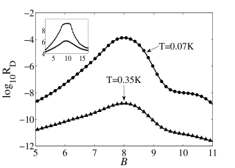
Figure 3: Drag resistance $R_{D}$ (in Ohms) between two identical films as in FIG. 2b of Ref. Sambandamurthy et al., 2004 vs. magnetic field $B$, according to the vortex pictureGalitski et al. (2005) (log scale); . The drag resistance has been smoothened to avoid discontinuity at the boundary between the metallic and the insulating phase. Center-to-center layer separation $a=25$nm, temperature $T=0.07$K and 0.35K. Insets: single layer magnetoresistance (magnetoresistance, log scale) reproduced according to the quantum vortex theory.. The parameters are tuned to make the magnetoresistance resemble the experimental data in FIG. 2b of Ref. Sambandamurthy et al., 2004. $R_{D}$ has a peak at the steepest point ($\sim 8$T) of the magnetoresistance, which is due to the fact that $R_{D}$ is proportional to the square of the slope of the magnetoresistance in the small magnetic field side of the peak. Also, $R_{D}$ is larger at lower temperature, because the magnetoresistance curve is then much steeper. Carrying out the experiments at even lower temperatures may further enhance the vortex drag effect.

Collecting the above results and the value of the vortex mass $m_{v}$ discussed in Appendix II.1, tuning the value of the vortex (spinon) contributions to the resistance $R_{v}$ ($R_{s}$) so that $R=R_{v}R_{s}/(R_{v}+R_{s})$ (see Ref. Galitski et al., 2005) resembles the resistance observed in the experiment of Ref. Sambandamurthy et al., 2004, and setting temperature to be 0.07K and 0.35K, we have calculated the drag resistance between two identical films with single layer resistance given by the inset of FIG.3, and with center-to-center layer separation 25nm. We assume that vortices form a Fermi liquid (thus (15) is applicable; however see also Appendix D) when $B<9$T, and a bosonic superfluid (thus (32) is used) when $B>9$T. We smoothen the drag resistance curve by convoluting it with a Gaussian function to avoid discontinuity across the phase boundary between the metallic phase and the insulating phase.

The results of vortex drag are summarized in FIG.3. One can see that The drag resistance has a peak at the steepest point ($\sim 8$T) of the magnetoresistance. This is due to the fact that in the vortex metal regime, the drag resistance is proportional to the square of the slope of the magnetoresistance. Also, the drag resistance is larger at lower temperature. This is because the magnetoresistance curve is much steeper as one approaches zero temperature(see (15)). For the film of Ref. Sambandamurthy et al., 2004, the sheet drag resistance is about $10^{-1}$ m$\Omega$ at its maximum, which is measurable despite challenging. We suggest to carry out experiments to even lower temperature, which should leads to a larger drag resistance. Using a Hall-bar shape sample would also amplify the result.

III drag resistance in the percolation picture

III.1 Review of the percolation picture of the magnetoreistance

Within the percolation picture of Ref. Dubi et al., 2006, it is argued that the non-monotonic magnetoresistance arises from the film breaking down to superconducting and normal regions (described as localized electron glass) Dubi et al. (2006). As the magnetic field increases, the superconducting region shrinks, and a percolation transition occurs. Once the normal regions percolate, electrons must try to enter a superconducting island in pairs, and therefore encounter a large Coulomb blockade absent in normal puddles. The magnetoresistance peak thus reflect the competition between electron transport though narrow normal regions, and the tunneling through superconducting islands.

This picture is captured using a resistor network description. Each site of the network has a probability $p$ to be normal, and $1-p$ to be superconducting; each link is assigned a resistance from the three values $R_{NN},\,R_{SS},\,R_{SN}$, that reflect whether the sites the link connects are normal (N), or superconducting (S). An increase of the magnetic field is assumed to only cause $p$ to increase. Since the normal region is described as disordered electron glass, $R_{NN}$, the resistance between two normal sites, is assumed to be of the form of hopping conduction:

$$R_{ij}\sim R_{N0}\exp{\left(\frac{2}{\xi_{loc}}+\frac{|\epsilon_{i}|+|\epsilon_{j}|+|\epsilon_{i}+\epsilon_{j}|}{k_{B}T}\right)},$$ (35)

where $\xi_{loc}$ is the localization length, and $\epsilon_{i}$ is the energy of the $i-$th site measured from the chemical potential (taken from a uniform distribution $[-W/2,W/2]$), and for simplicity we allow only nearest neighbor hopping. The resistance between two superconducting sites, $R_{SS}$, is taken to be very small, but still nonzero, and vanishes as $T\sim T^{\alpha}\rightarrow 0$. Most importantly, the resistance between one normal site and a neighboring superconducting site, $R_{SN}$, is assumed activated:

$$R_{SN}\sim R_{SN0}\exp\left(\frac{E_{c}}{k_{B}T}\right)$$ (36)

to model the charging energy electrons need to pay to enter a superconducting island.

We have reproduced the work of Ref. Dubi et al., 2006 where the parameters of this model are chosen to reproduce the magneto-resistance curves and temperature dependence observed in the strong-insulator InO sample Sambandamurthy et al. (2004). The total resistance vs. the probability of normal metal (assumed to increase with increasing magnetic field) is shown in the inset of FIG.4. Indeed, the peak of the magnetoresistance can be explained by this theory. However, as we demonstrate now, this theory predicts a very different behavior for the drag resistance.

III.2 Calculation of drag resistance within the percolation picture

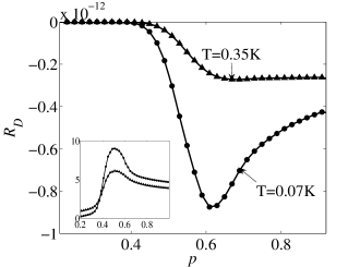
Figure 4: Drag resistance $R_{D}$ (in Ohms) between two identical films as in FIG. 2b of Ref. Sambandamurthy et al., 2004 vs. normal metal percentage $p$ (corresponding to normal magnetic field), according to the percolation pictureDubi et al. (2006). Center-to-center layer separation $a=25$nm, temperature $T=0.07K$ and $0.35K$. Insets: single layer magnetoresistance (magnetoresistance, log scale) reproduced according to the percolation theory. The parameters are tuned to make the magnetoresistance resemble the experimental data in FIG. 2b of Ref. Sambandamurthy et al., 2004. The sign of the voltage drop of the passive layer is opposite to that of the driving layer, and the maximum magnitude value of $R_{D}$ is much smaller, $\sim 10^{-12}\Omega$.

To calculate $R_{D}$, we first follow Ref. Dubi et al., 2006 and tune the parameters to make the single layer resistance resemble the experimental data in FIG. 2(b) of Ref. Sambandamurthy et al., 2004: $\xi_{loc}=0.1$, $W=0.4$K, $E_{c}=0.6$K, $R_{SN0}\sim 10^{6}\Omega$, and $R_{N0}\sim 10^{-5}\Omega$. Next, we place one such network (active layer) on top of another one (passive layer). Each link is treated as a subsystem, which might induce a drag voltage (an emf) $\varepsilon=IR_{D}$ in the link under it in the passive layer. When a link is between two normal (or superconducting) sites, it is treated as a disorder localized electron glass (or superconductor). In Appendix E, we find $R_{D}$ between two localized electron glass separated by vacuum is:

$$R_{D}\approx\frac{1}{96\pi^{2}}\frac{R_{1}R_{2}}{\hbar/e^{2}}\frac{T^{2}}{(e^{2}nad)^{2}}\ln\frac{1}{2x_{0}}.$$ (37)

Here, $n\approx 5\times 10^{20}$cm^-3 is the typical carrier density of InOSteiner and Kapitulnik (2005), $d=20$nm is the film thickness, $a=25$nm is the center-to-center layer separation, $R_{1,2}$ are the resistances of the two normal-normal(NN) links, $x_{0}=a/(2\pi e^{2}\nu d\xi^{2})$ where $\nu$ is the density of states and $\xi\approx 1$nm is the localization length. The value of the localization length $\xi$ is estimated by following Ref. Dubi et al., 2006 to take $\xi\sim 0.1\times$ plaquette size (reflecting the fact that it is a disordered insulator), and we estimate the plaquette size as the superconducting coherence length $\sim 10$nm. Although this estimation of localization length is crude, the drag resistance $R_{D}$ has only logarithmic dependence on it in (37). Setting $T=0.07$K, and $R_{1}=R_{2}=10^{5}\Omega$, we can estimate $R_{D}\sim 10^{-12}\Omega$.

On the other hand, we will show in Appendix F that a genuine (i.e., without mobile vortices) superconductor has no drag effect at all in a resistor network, either when it is aligned with another superconductor link or a normal link. Thus, drag effects associated with a superconducting link can only come from vortices. However, The small resistance for the superconducting islands in this theory implies that vortices in the superconducting islands, if any, have very low mobility. If two superconducting links are vertically aligned, we can estimate the drag resistance due to mobile vortices using our vortex drag result (15): roughly $R_{D}\propto R^{2}$, for $R\sim 10^{9}\Omega$ we obtained $R_{D}\sim 10^{-4}\Omega$, therefore for $R\sim 1\Omega$ we have $R_{D}\sim 10^{-20}\Omega$, which is negligible compared to the Coulomb drag resistance between two NN links $\sim 10^{-12}\Omega$. Finally, Ref. Narayan, 2003 has shown that a current off the plane where vortices reside does not exert any force on vortices. By Newton’s third law or equivalently the Kubo formula for the drag conductance, this also implies that moving vortices does not exert any DC emf in another layer. Therefore, there is no drag effect when a NN link is aligned with a SS link. Consequently, the Coulomb drag between two vertically aligned NN links (Eqn. (37)) dominates the drag effect.

Thus, we solve the Kirchoff’s equations for the two layers, and obtain the voltage drop and thereby the drag resistance. The results are shown in FIG. 4, with $T=0.07$K and $0.35$K, film-thickness 20nm, and the center-to-center interlayer distance 25nm. We observe that the sign of the voltage drop of the passive layer is opposite to that of the driving layer (not shown in the Figure), as expected and explained in the introduction, and the maximum magnitude of the drag resistance is around $10^{-12}\Omega$, indeed much smaller than that in the vortex paradigm.

IV Discussion on the drag resistance in the phase glass theory

A third theory, namely the phase glass theoryDalidovich and Phillips (2002); Wu and Phillips (2006), focuses on the nature of the metallic phase intervening the superconducting and insulating state. In this theory, the system is described as interacting bosons (Cooper pairs), but it is argued that the glassy phase is in fact a Bose metal, due to the coupling to the glassy landscape.

Specifically, Ref. Dalidovich and Phillips, 2002 has studied the quantum rotor model

$$H=-E_{c}\sum_{i}\left(\frac{\partial}{\partial\theta_{i}}\right)^{2}-\sum_{\langle i,j\rangle}J_{ij}\cos(\theta_{i}-\theta_{j}),$$ (38)

where the Josephson coupling $J_{ij}$ obeys a Gaussian distribution with nonzero mean. This model is appears to exhibit three phases: superconducting phase, phase glass phase, and a Mott insulator phase. Ref. Dalidovich and Phillips, 2002 has employed replica trick to obtain the Landau theory of the the phase glass phase near the glass-superconductor-transition critical point, and has calculated the conductance in this regime. It was found that in this regime the DC conductance is actually finite at zero temperature. For completeness, we note that Ref. Ikeda, 2007 argued against these results and obtained infinite conductance instead.

This analysis has recently been extended to include the external perpendicular magnetic fieldWu and Phillips (2006), which is more relevant to the experiments on the magnetic field tuned transition. However, Ref.Wu and Phillips, 2006 has only studied the regime of small magnetic field where one just enters the resistive glassy phase and left out issues such as the peak in the magnetoresistance. Therefore, we leave a complete analysis to future work and simply observe that according to this theory, the resistive state is a glassy phase where phase variables $\theta_{i}$’s of the bosons are ordered locally. In other words, there are no mobile vortices moving around. Consequently, the current coupling as we considered in the vortex drag should is absent, and the Coulomb interaction should dominate the drag effect. Therefore, we expect that the sign of the drag voltage is opposite to the voltage drop of the driving layer, as we discussed in the introduction to be a general feature of the Coulomb drag, and the magnitude of the drag resistance should be small. This is in part because for a bosonic system, the phase space available for excitations is much smaller than fermionic systems due to the absence of a Fermi surface.

V summary and discussion

One of the most exciting possiblities is that the SIT in amorphous thin films realizes the vortex condensation scenario Fisher and Lee (1989); Fisher (1990); Galitski et al. (2005). The amorphous-films Giaver transformer experiment Zou et al. (2009), would be able to measure a distinct signature of mobile vortices, which is a drag resistance opposite in its direction to that of coulomb drag. Therefore such a measurement would able to disclose whether the vortex paradigm is suitable for explaining the complex phase diagram of amorphous films in a normal manetic field, or whether the percolation paradigm is indeed more appropriate. We provide a detailed computation of the drag resistance according to the vortex theories of Ref. Fisher, 1990; Galitski et al., 2005 and the percolation theory of Ref. Dubi et al., 2006. The drag resistance implied by the phase glass modelDalidovich and Phillips (2002); Wu and Phillips (2006) is also briefly discussed. We find that vortex picture predicts a drag resistance orders of magnitude stronger than non-vortex pictures. In addition, the drag resistance and the single layer resistance have the same sign according to the vortex picture, but the opposite sign for non-vortex pictures. Therefore, drag resistance measurement are indeed able to distinguish different theoretical paradigms qualitatively.

We considered specifically a bilayer device which will contain two identical films as in Ref. Sambandamurthy et al., 2004 with $25$nm layer separation and at $0.07$K. A calculation within the vortex paradigm yields a drag resistance $R_{D}\sim 10^{-4}\Omega$ at its maximum value. This drag arises solely from the attractive interaction of the demagnetizing currents of vortices. The value we find is probably near the limit of measurability; we suggest, however, to carry out experiments at even lower temperature, in which case the single layer magnetoresistance is even steeper, and the drag resistance should be larger. Within the percolation picture of Ref. Dubi et al., 2006, the dominating drag effect is the drag between two vertically aligned normal regions in the different layers. For two identical films as in Ref. Sambandamurthy et al., 2004 with $25$nm layer separation at $0.07$K, we find the drag resistance $R_{D}\sim 10^{-12}\Omega$ at its maximum value, which is indeed orders of magnitude smaller than the drag resistance predicted by the vortex picture. Also, we find the sign of the drag resistance is the opposite of that of the single layer resistance, as expected.

The answer we find should not depend crucially on the details of the microscopic picture which we use. If vortices are not responsible for the inhibitive resistance which the films display, then drag effects will appear primarlily due to Coulomb repulsion of single electrons. This drag effect will be low because of the relatively high electronic density in the films. On the other hands, if vortices are responsible for the large resistance in the intermediate magnetic fields leading to the insulating phase, then they will produce a drag opposite in its direction to the Coulomb drag. To carry out the vortex drag calculation in the metallic phase intervening between the superconducting and insulating phase we used the picture of Ref. Galitski et al., 2005, which treats the vortices as fermionic diffusive particles. This picture is justified due to the strong long-ranged interactions within the vortex liquid, which render the question of statistics secondary, intuitively, since vortices rarely encircle each other. Nevertheless, to demonstrate the universality of our results, we also carried out the drag calculation in the metalic phase assuming that the vortices are hard core disks, and obtained essentially the same answer (c.f. App. D).

Indeed our strongest results are obtained in the intermediate-field metallic phase. The controversy surrounding this phase requires some special attention. First, we note that all experiments of thin amorphous films exhibit a saturation of the resistance at temperature below about $100$mK at intermediate resistances. This is clearly seen in, e.g, the resistance vs. field traces which overlap at subsequent temperature sweeps as in Fig.2b of Ref. Sambandamurthy et al., 2004. Second, there are reasons to believe that this saturation is not the result of failure to cool electrons. Resistances that are too low or too high continue to change as the temperature is lowered. But the two heating mechanisms most likely are current heating, with power $\sim I^{2}R$, and therefore affecting the highest temperatures, and ambient RF heating, which would have a voltage-biased power $\sim V^{2}/R$, and therefore most effective in the lowest resistances. Neither mechanism explains resistance saturation at intermediate temperatures. Furthermore, experiments on Tantalum films show distinct signatures in the metallic regime which disappear in the insulating and superconducting regimes, and also distinguish it from the thermally-destroyed superconducting phaseSeo et al. (2006). Third, even if the metallic behavior of the films is a finite temperature phenomena, within the vortex paradigm, the resistance still arises due to vortex motion. Therefore the drag calculated within this paradigm using a diffusive vortex model should still be adequate, and our results do not depend crucially on the existence of a zero-temperature intervening metallic state.

The signatures we expect to find in the proposed magnetic and Coulomb drag measurements are not large. Incorporating interlayer electron and Josephson tunneling will increase both the vortex-drag effect and the competing Coloumb drag effects. As we point out here, the drag signature of vortex motion, or single electrons or Cooper-pairs motion will have opposite signs. Quite possibly, allowing interlayer tunneling will render both drag effects measurable. Indeed, such a setup will be a deviation from standard drag measurements where charge transfer between layers is forbidden. Nevertheless, a careful choice of tunneling strength and sample geometry will make such experiments plausible and useful. We intend to analyze the vortex and Coloumb drag in the presence of interlayer tunneling in future work.

Appendix A The determination of the vortex mass

In this appendix, we demonstrate in detail the derivation of the vortex-boson duality for a single layer and discuss the value of the vortex mass. Our starting point is the following partition function for Cooper pairs:

$$\mathcal{Z}=\int\mathcal{D}\rho\mathcal{D}\theta\mathcal{D}\vec{A}e^{-S},$$ (39)

where the action $S$ is

$$S = \int_{0}^{\beta}\mathrm{d}\tau\left\{\int\mathrm{d}^{2}r(\hbar\rho\partial_{\tau}\theta+H_{0}+H_{int})\right\},$$

$$H_{0} = \int\mathrm{d}^{2}r\frac{\rho_{s}}{2\hbar^{2}}\left(\hbar\nabla\theta-\frac{2e}{c}\vec{A}_{ext}-\frac{2e}{c}\vec{A}\right)^{2}$$

$$+ \frac{1}{4\pi}\int\mathrm{d}^{3}r\vec{B}^{2},$$

$$H_{int} = \int\mathrm{d}^{2}r\int\mathrm{d}^{2}r^{\prime}\frac{1}{2}\rho(r)V(r-r^{\prime})\rho(r^{\prime}).$$ (40)

Here, $\rho$ and $\theta$ are the density and phase fluctuation of the Cooper pair field, respectively, $\vec{A}$ is the fluctuating electromagnetic field, and $\vec{A}_{ext}$ is the applied external electromangetic field, typically a perpendicular magnetic field. $V(r)=(2e)^{2}/r$ (whose 2d Fourier transform would be $2\pi(2e)^{2}/k$) is the Coulomb interaction between Cooper pairs. $\rho_{s}$ is the bare stiffness for phase fluctuations. The value of $\rho_{s}$ can be determined approximately by the zero-field Kosterlitz-Thouless temperature $T_{KT}$:

$$T_{KT}=\frac{\pi}{2}\rho_{s}.$$ (41)

The 2d number current of Cooper pairs is

$$\vec{j}=\frac{\rho_{s}}{\hbar^{2}}\left(\hbar\nabla\theta-\frac{2e}{c}\vec{A}_{ext}-\frac{2e}{c}\vec{A}\right).$$ (42)

One can introduce the dynamical field $\vec{j}$ by Hubbard-Stratonavich transformation (or Villain transformation in the lattice version of this derivation) and transform $\mathcal{Z}$ to be

$$\mathcal{Z}=\int\mathcal{D}\rho\mathcal{D}\theta\mathcal{D}\vec{j}\mathcal{D}\vec{A}e^{-S},$$ (43)

where

$$S = \sum_{\omega,\vec{q}}\left\{-i\hbar\omega\rho\theta+\frac{1}{2}\rho V\rho+\frac{\hbar^{2}}{2\rho_{s}}\vec{j}^{2}\right.$$ (44)

$$+ i\vec{j}\cdot\left(\hbar(\nabla\theta)_{q}-\frac{2e}{c}\vec{A}_{ext}-\frac{2e}{c}\vec{A}(\vec{q},z=0)\right)$$

$$+ \left.\int\frac{dk_{z}}{2\pi}\frac{q^{2}+k_{z}^{2}}{4\pi}\vec{A}^{2}(\vec{q},k_{z})\right\}.$$

Here, $i$ is the imaginary number unit, $\vec{q}$ is the in-plane 2d wave vector, while $k_{z}$ is the 3rd wave vector component perpendicular to the plane, and subscripts $\vec{q}$ mean Fourier transformed variables. Next we split the $\theta$ field into a smooth part $\theta_{s}$ and a vortex part $\theta_{v}$: $\theta=\theta_{s}+\theta_{v}$. Afterwards one can integrate out $\theta_{s}$ to obtain the continuity constraint:

$$\mathcal{Z}=\int\mathcal{D}\rho\mathcal{D}\vec{j}\mathcal{D}\theta_{v}\mathcal{D}\vec{A}\delta(\partial_{t}\rho+\nabla\cdot\vec{j})e^{-S},$$ (45)

where

$$S =\sum_{\omega,\vec{q}}\left\{-i\hbar\omega\rho\theta_{v}+\frac{1}{2}\rho V\rho+\frac{\hbar^{2}}{2\rho_{s}}\vec{j}^{2}\right.$$

$$+i\vec{j}\cdot\left(\hbar(\nabla\theta_{v})_{q}-\frac{2e}{c}\vec{A}_{ext}-\frac{2e}{c}\vec{A}(\vec{q},z=0)\right)$$

$$+\left.\int\frac{dk_{z}}{2\pi}\frac{q^{2}+k_{z}^{2}}{4\pi}\vec{A}^{2}(\vec{q},k_{z})\right\}.$$

Furthermore, noting that $\vec{A}(\vec{q},z=0)=\int\frac{dk_{z}}{2\pi}\vec{A}(\vec{q},k_{z})$, one can integrate out $\vec{A}$ in its transverse gauge, and the action $S$ now reads

$$S = \sum_{\omega,\vec{q}}\left\{-i\hbar\omega\rho\theta_{v}+\frac{1}{2}\rho V\rho+i\vec{j}\cdot\left(\hbar(\nabla\theta_{v})_{q}-\frac{2e}{c}\vec{A}_{ext}\right)\right.$$ (46)

$$+ \left.\frac{\hbar^{2}}{2\rho_{s}}\left(1+\frac{q_{c}}{q}\right)\vec{j}^{2}\right\},$$

where $q_{c}$ is the inverse of the 2d Pearl screening lengthPearl (1964), and typically it is much smaller than $1/L$, where $L$ is the sample size.

The continuity constraint is solved by defining a new gauge field $a_{\mu}=(a_{0},\vec{a})$ such that

$$j_{\mu}=\frac{1}{\eta}\epsilon_{\mu\nu\eta}\partial_{\nu}a_{\eta},$$ (47)

where $j_{\mu}=(c^{*}\rho,\vec{j})$ and $\partial_{\mu}=(\frac{1}{c^{*}}\partial_{\tau},\nabla)$, and the value of constant $\eta$ and the ”speed of light” $c^{*}$ are to be determined. Writing in components, (47) is

$$\vec{e}=\eta\vec{j}\times\hat{z},\qquad b=\eta c^{*}\rho,$$ (48)

where $\vec{e}$ and $b$ are the dual ”electric field” and ”magnetic field” associated with $\alpha$, respectively. To fix $\eta$ and $c^{*}$, we require

$$\frac{1}{4\pi}\vec{e}^{2}=\frac{\hbar^{2}}{2\rho_{s}}\left(1+\frac{q_{c}}{q}\right)\vec{j}^{2},\qquad\frac{1}{4\pi}b^{2}=\frac{1}{2}\rho V\rho,$$ (49)

thus

$$\eta\equiv\sqrt{\frac{2\pi\hbar^{2}}{\rho_{s}}\frac{q+q_{c}}{q}},\qquad c^{*}=\sqrt{\frac{2\pi(2e)^{2}\rho_{s}}{(q+q_{c})\hbar^{2}}}.$$ (50)

Using (47), we express the partition function $\mathcal{Z}$ as

$$\mathcal{Z}=\int\mathcal{D}\vec{a}\mathcal{D}a_{0}\mathcal{D}\theta_{v}e^{-S},$$ (51)

where

$$S = \sum_{\omega,\vec{q}}\left\{\frac{1}{\eta}\epsilon_{\mu\nu\eta}q_{\nu}a_{\eta}\left(\hbar(\partial_{\mu}\theta_{v})_{q}-\frac{2e}{c}A^{ext}_{\mu}\right)\right.$$ (52)

$$+ \left.\frac{1}{4\pi}(\omega^{2}-c_{*}^{2}q^{2})\left(\frac{\vec{a}}{c}_{*}\right)^{2}+\frac{q^{2}}{4\pi}a_{0}^{2}\right\}.$$

Integrating by parts, and noting the definition of the vortex current density

$$j^{v}_{\mu}=\frac{1}{2\pi}\epsilon_{\mu\nu\eta}\partial_{\nu}\partial_{\eta}\theta^{v},$$ (53)

we obtain

$$S = \sum_{\omega,\vec{q}}\left\{-e^{*}ia_{0}\left(\rho_{v}-\frac{B_{ext}}{\Phi_{0}}\right)+ie^{*}\vec{j}^{v}\cdot\frac{\vec{a}}{c^{*}}\right.$$ (54)

$$+ \left.\frac{1}{4\pi}(\omega^{2}-c_{*}^{2}q^{2})\left(\frac{\vec{a}}{c}_{*}\right)^{2}+\frac{q^{2}}{4\pi}a_{0}^{2},\right\}.$$

where $\Phi_{0}=hc/(2e)$, and the ”dual charge” of vortices is

$$e^{*}=\frac{2\pi\hbar}{\eta}=\sqrt{2\pi\rho_{s}}\sqrt{\frac{q}{q+q_{c}}}.$$ (55)

In the above, we have assumed that the only external electromagnetic field is a perpendicular magnetic field $B_{ext}$.

The magnitude of the Magnus force, which now appears as the electric force, can be easily verified:

$$F = e^{*}\times|\vec{e}|=\frac{2\pi\hbar}{\eta}\times\eta j=hj,$$ (56)

as expected.

Introducing a vortex field $\psi_{v}$ and making the action explicitly gauge-invariant, we write the action as

$$S =\sum_{\vec{q},\omega}\left\{\delta\rho_{v}(-\hbar i\omega\phi-ie^{*}a_{0})+\frac{1}{2m_{v}}\left[\left(\hbar\vec{q}-e^{*}\frac{\vec{a}}{c_{*}}\right)\psi_{v}\right]^{2}\right.$$

$$\qquad+\left.\frac{1}{4\pi}(\omega^{2}-c_{*}^{2}q^{2})\left(\frac{\vec{a}}{c_{*}}\right)^{2}+\frac{q^{2}}{4\pi}a_{0}^{2}\right\},$$ (57)

where $\delta\rho_{v}=\rho_{v}-\frac{B_{ext}}{\Phi_{0}}$, and we have introduced the vortex mass $m_{v}$. Integrating out $a_{0}$, one obtains

$$S = \sum_{\vec{q},\omega}\left\{-\delta\rho_{v}\hbar i\omega\phi+\frac{1}{2}\delta\rho_{v}U\delta\rho_{v}\right.$$ (58)

$$+ \frac{1}{2m_{v}}\left[(\hbar\vec{q}-e^{*}\frac{\vec{a}}{c_{*}})\psi_{v}\right]^{2}$$

$$+ \left.\frac{1}{4\pi}(\omega^{2}-c_{*}^{2}q^{2})\left(\frac{\vec{a}}{c_{*}}\right)^{2}\right\},$$

where

$$U(q)=\frac{\Phi_{0}^{2}q_{c}}{2\pi}\frac{1}{q(q+q_{c})}$$ (59)

is the well-known Pearl interaction potentialPearl (1964).

In the insulating phase, i.e., the vortex condensed phase with vortex superfluid stiffness $\rho_{vs}$, we have

$$S = \sum_{\vec{q},\omega}\left\{-\delta\rho_{v}\hbar i\omega\phi+\frac{\rho_{vs}}{2\hbar^{2}}\left(i\hbar\vec{q}\phi-e^{*}\frac{\vec{a}}{c_{*}}\right)^{2}\right.$$ (60)

$$+ \left.\frac{1}{2}\delta\rho_{v}U\delta\rho_{v}+\frac{1}{4\pi}(\omega^{2}-c_{*}^{2}q^{2})\left(\frac{\vec{a}}{c_{*}}\right)^{2}\right\}.$$

Due to the Higgs mechanism in this ”symmetry broken phase”, the gap of the two modes in the vortex superfluid phase coincide to be

$$E_{gap}=\sqrt{2\pi\rho_{vs}e_{*}^{2}}\approx 2\pi\sqrt{\rho_{vs}\rho_{s}}$$ (61)

for $q_{c}\ll L^{-1}$. Roughly speaking the two modes correspond to a density fluctuation of the vortices, or of the underlying Cooper-pairs Deep in the insulating phase, i.e., near the peak of the magnetoresistance, the vortex stiffness is simply

$$\rho_{vs}=\hbar^{2}\frac{n_{v}}{m_{v}},$$ (62)

where the vortex density $n_{v}\equiv B/\Phi_{0}$. Therefore, in this regime we have

$$E_{gap}=2\pi\hbar\sqrt{\frac{n_{v}}{m_{v}}\rho_{s}}.$$ (63)

Since the gauge field $a_{\mu}$ is actually the fluctuation of Cooper pairs, we conjecture that its gap $E_{gap}$ can be identified with the activation gap observed in the experiments of Ref. Sambandamurthy et al., 2004; Steiner and Kapitulnik, 2005 near the insulating peak. Ref.Sambandamurthy et al., 2004; Steiner and Kapitulnik, 2005 have also found that with increasing disorder strength, the ratio $E_{gap}/T_{KT}$ is enhanced. This is natural from our expression (63): dividing (63) by (41), we have

$$\frac{E_{gap}}{T_{KT}}=4\hbar\sqrt{\frac{n_{v}}{m_{v}}\frac{1}{\rho_{s}}};$$ (64)

increasing disorder makes vortices more mobile and thereby suppresses the vortex mass $m_{v}$ Wallin et al. (1994); it also suppresses the superfluid stiffness $\rho_{s}$. Therefore, $E_{gap}/T_{KT}$ is larger for more disordered sample.

Since there is still controversy over its theoretical value, we chose to use the experimental value of $E_{gap}$ as an input to deduce the vortex mass from (63). Combining (41), we can express the vortex mass $m_{v}$ as a function of observable quantities:

$$m_{v}=\frac{8\pi n_{v}T_{KT}}{E_{gap}^{2}}.$$ (65)

Again, the vortex density $n_{v}=B/\Phi_{0}$. For the InO film of Ref. Sambandamurthy et al., 2004, $T_{KT}\approx 0.5$K, and $E_{gap}\approx 1.6$K at $B=9$T. Plugging these into (65), we obtain $m_{v}\approx 19m_{e}$ where $m_{e}$ is the bare electron mass. For comparison, this value is not far from that of the so-called core mass of dirty superconductorsKuprianov and Likharev (1975); Blatter et al. (1991); Duan and Leggett (1992); Sonin et al. (1998) $m\sim(k_{F}d)m_{e}\sim 49m_{e}$ if we use carrier density $\sim 5\times 10^{20}$cm^-3 and $d\sim 20$nm (see Ref. Sambandamurthy et al., 2004; Steiner and Kapitulnik, 2005).

Appendix B The field theory derivation of the vortex interaction potentials in bilayers

For identical bilayer superconducting thin films separated by a (center-to-center) distance $a$, we have the following partition function for Cooper pairs:

$$\mathcal{Z}=\int\mathcal{D}\rho_{1}\mathcal{D}\rho_{2}\mathcal{D}\theta_{1}\mathcal{D}\theta_{2}\mathcal{D}\vec{A}e^{-S},$$ (66)

where

$$S = \int_{0}^{\beta}\mathrm{d}\tau\left\{\int\mathrm{d}^{2}r\sum_{n=1,2}\hbar\rho_{n}\partial_{\tau}\theta_{n}+H_{0}+H_{int}\right\},$$

$$H_{0} = \int\mathrm{d}^{2}r\sum_{n=1,2}\frac{\rho_{s}}{2\hbar^{2}}\left(\hbar\nabla\theta_{n}-\frac{2e}{c}\vec{A}_{ext}-\frac{2e}{c}\vec{A}\right)^{2}$$

$$+ \frac{1}{4\pi}\int\mathrm{d}^{3}r\vec{B}^{2},$$

$$H_{int} = \int\mathrm{d}^{2}r\int\mathrm{d}^{2}r^{\prime}\frac{1}{2}\sum_{n=1,2}\rho_{n}(r)V_{i}(r-r^{\prime})\rho_{n}(r^{\prime})$$

$$+ \rho_{1}(r)V_{e}(r-r^{\prime})\rho_{2}(r^{\prime}),$$

where $\rho_{n}$ and $\theta_{n}$ are the density and phase fluctuation of the $n-$th layer Cooper pair field, respectively, $A$ and $A_{ext}$ are the fluctuating and external part of the electromagnetic field, respectively. The intralayer Coulomb interaction $V_{i}(r)=(2e)^{2}/r$ (whose 2d Fourier transform would be $2\pi(2e)^{2}/q$), and the interlayer Coulomb interaction $V_{e}(r)=(2e)^{2}/\sqrt{r^{2}+a^{2}}$ (whose 2d Fourier transform is $2\pi(2e)^{2}/qe^{-qa}$). $\rho_{s}$ is the superfluid phase stiffness of each layer.

Similar to the single layer case in Appendix A, we can again introduce Hubbard-Stratonavich fields $\vec{j}_{1,2}$, split $\theta$’s into smooth parts $\theta_{s}$ and vortex parts $\theta_{v}$, integrate out $\theta_{s}$ and $\vec{A}$, and obtain

$$\mathcal{Z} = \int\mathcal{D}\rho_{1}\mathcal{D}\rho_{2}\mathcal{D}\theta^{v}_{1}\mathcal{D}\theta^{v}_{2}\mathcal{D}\vec{j}_{1}\mathcal{D}\vec{j}_{2}$$ (67)

$$\times \delta(\partial_{t}\rho_{1}+\nabla\cdot\vec{j}_{1})\delta(\partial_{t}\rho_{2}+\nabla\cdot\vec{j}_{2})e^{-S}$$

where

$$S = \sum_{\omega,\vec{q}}\left\{-i\hbar\omega\rho_{1}\theta^{v}_{1}+i\vec{j}_{1}\cdot\left(\hbar(\nabla\theta^{v}_{1})_{q}-\frac{2e}{c}\vec{A}_{ext}\right)\right.$$ (68)

$$- i\hbar\omega\rho_{2}\theta^{v}_{2}+i\vec{j}_{2}\cdot\left(\hbar(\nabla\theta^{v}_{2})_{q}-\frac{2e}{c}\vec{A}_{ext}\right)$$

$$+ \frac{1}{2}\rho_{1}V_{i}\rho_{1}+\frac{1}{2}\rho_{2}V_{i}\rho_{2}+\rho_{1}V_{e}\rho_{2}$$

$$+ \frac{\hbar^{2}}{2\rho_{s}}\left(1+\frac{q_{c}}{q}\right)\vec{j}_{1}^{2}+\frac{\hbar^{2}}{2\rho_{s}}\left(1+\frac{q_{c}}{q}\right)\vec{j}_{2}^{2}$$

$$+ \left.\frac{\hbar^{2}}{\rho_{s}}\frac{q_{c}}{q}e^{-qa}\vec{j}_{1}\cdot\vec{j}_{2}\right\}.$$

The difference from the single layer case is that now the continuity constraint is solved by introducing two new gauge fields $\alpha_{\mu}=(\alpha_{0},\vec{\alpha})$ and $\beta_{\mu}=(\beta_{0},\vec{\beta})$ such that

$$j_{1\mu}+j_{2\mu} = \frac{1}{\eta_{1}}\epsilon_{\mu\nu\eta}\partial_{\nu}\alpha_{\eta},$$

$$j_{1\mu}-j_{2\mu} = \frac{1}{\eta_{2}}\epsilon_{\mu\nu\eta}\partial_{\nu}\beta_{\eta};$$

Denoting the electric field and the magnetic field associated with $\alpha_{\mu}(\beta_{\mu})$ are $\vec{e}_{1}$ and $b_{1}$ ($\vec{e}_{2}$ and $b_{2}$), respectively, we have

$$\vec{e}_{1} = \eta_{1}(\vec{j}_{1}+\vec{j}_{2})\times\hat{z},\qquad b_{1}=\eta_{1}c_{*1}(\rho_{1}+\rho_{2})$$

$$\vec{e}_{2} = \eta_{2}(\vec{j}_{1}-\vec{j}_{2})\times\hat{z},\qquad b_{2}=\eta_{2}c_{*2}(\rho_{1}-\rho_{2}).$$ (69)

To fix $\eta_{1,2}$ and the ”speeds of light” $c_{*1,2}$, we require

$$\frac{1}{4\pi}(\vec{e}_{1}^{2}+\vec{e}_{2}^{2})=\frac{\hbar^{2}}{2\rho_{s}}\left(1+\frac{q_{c}}{q}\right)(\vec{j}_{1}^{2}+\vec{j}_{2}^{2})+\frac{\hbar^{2}}{\rho_{s}}\frac{q_{c}}{q}e^{-qa}\vec{j}_{1}\cdot\vec{j}_{2};$$

$$\frac{1}{4\pi}(b_{1}^{2}+b_{2}^{2})=\frac{1}{2}\rho_{1}V_{i}\rho_{1}+\frac{1}{2}\rho_{2}V_{i}\rho_{2}+\rho_{1}V_{e}\rho_{2},$$

thus for $n=1,2$,

$$\eta_{n} = \sqrt{\frac{\pi\hbar^{2}}{\rho_{s}}\left(1+\frac{q_{c}}{q}\left(1-(-1)^{n}e^{-qa}\right)\right)},$$ (70)

$$c_{*n} = c\sqrt{\frac{q_{c}(1-(-1)^{n}e^{-qa})}{q+q_{c}(1-(-1)^{n}e^{-qa})}}.$$ (71)

Using (B) and (53), we can again integrate by parts and express the partition function $\mathcal{Z}$ as

$$\mathcal{Z}=\int\mathcal{D}\alpha\mathcal{D}\beta\mathcal{D}\theta_{v1}\mathcal{D}\theta_{v2}e^{-S},$$ (72)

where

$$S = \sum_{\omega,\vec{q}}i\left\{-(e_{1}^{*}\alpha_{0}+e_{2}^{*}\beta_{0})\left(\rho_{v1}-\frac{B_{ext}}{\Phi_{0}}\right)\right.$$ (73)

$$- i(e_{1}^{*}\alpha_{0}-e_{2}^{*}\beta_{0})\left(\rho_{v2}-\frac{B_{ext}}{\Phi_{0}}\right)$$

$$+ i\vec{j}_{v1}\cdot(e_{1}^{*}\frac{\vec{\alpha}}{c_{*1}}+e_{2}^{*}\frac{\vec{\beta}}{c_{*2}})+i\vec{j}_{v2}\cdot(e_{1}^{*}\frac{\vec{\alpha}}{c_{*1}}-e_{2}^{*}\frac{\vec{\beta}}{c_{*2}})$$

$$+ \frac{1}{4\pi}(\omega^{2}-c_{*1}^{2}q^{2})\left(\frac{\vec{\alpha}}{c_{*1}}\right)^{2}+\frac{q^{2}}{4\pi}\alpha_{0}^{2}$$

$$+ \left.\frac{1}{4\pi}(\omega^{2}-c_{*2}^{2}q^{2})\left(\frac{\vec{\beta}}{c_{*2}}\right)^{2}+\frac{q^{2}}{4\pi}\beta_{0}^{2}\right\},$$

and for $n=1,2$, the dual ”charges” of the vortices are

$$e_{n}^{*} = \frac{\pi\hbar}{\eta_{n}}=\sqrt{\pi\rho_{s}}\sqrt{\frac{q}{q+q_{c}(1-(-1)^{n}e^{-qa})}},$$

When a (number) current bias $\vec{j}_{1}$ is applied in layer 1, the force on a vortex in this layer is

$$F =e_{1}^{*}\times|\vec{e}_{1}|+e_{2}^{*}\times|\vec{e}_{2}|=e_{1}^{*}\eta_{1}|\vec{j}_{1}|+e_{2}^{*}\eta_{2}|\vec{j}_{1}|$$

$$=h|\vec{j}_{1}|,$$

and the force on a vortex in the other layer is

$$F =e_{1}^{*}\times|\vec{e}_{1}|-e_{2}^{*}\times|\vec{e}_{2}|=e_{1}^{*}\eta_{1}|\vec{j}_{1}|-e_{2}^{*}\eta_{2}|\vec{j}_{1}|$$

$$=0,$$

as expected.

Again, introducing vortex fields $\psi_{v1}$ and $\psi_{v2}$ for each layer and making the action explicitly gauge-invariant, we can write the action as in

$$S =\sum_{\vec{q},\omega}\left\{\sum_{n=1,2}\left[\frac{\left(\left(\hbar\vec{q}-e_{1}^{*}\frac{\vec{\alpha}}{c^{*}_{1}}+(-1)^{n}e_{2}^{*}\frac{\vec{\beta}}{c^{*}_{2}}\right)\psi_{vn}\right)^{2}}{2m_{v}}\right.\right.$$

$$+\left.\delta\rho_{vn}\left(-i\hbar\omega\phi_{n}-ie_{1}^{*}\alpha_{0}+(-1)^{n}ie_{2}^{*}\beta_{0}\right)\right]$$

$$+\frac{1}{4\pi}(\omega^{2}-c_{*1}^{2}q^{2})\left(\frac{\vec{\alpha}}{c^{*}_{1}}\right)^{2}+\frac{1}{4\pi}(\omega^{2}-c_{*2}^{2}q^{2})\left(\frac{\vec{\beta}}{c^{*}_{2}}\right)^{2}$$

$$+\left.\frac{q^{2}}{4\pi}\alpha_{0}^{2}+\frac{q^{2}}{4\pi}\beta_{0}^{2}\right\}.$$ (75)

Integrating out $\alpha_{0}$ and $\beta_{0}$, one obtains the intralayer vortex interaction potential

$$U_{i}(q) =\frac{\Phi_{0}^{2}q_{c}}{2\pi}\frac{q+q_{c}}{q(q^{2}+2q_{c}q+q_{c}^{2}(1-e^{-2qa}))},$$ (76)

and interlayer vortex interaction potential

$$U_{e}(q) =-\frac{q_{c}}{q+q_{c}}e^{-qa}U_{i}.$$ (77)

Which concludes the field-theory derivation of the interaction potential.

Appendix C Classical derivation of the vortex interaction potential

In this appendix, we present an alternative way of deriving the vortex interaction potential between two vortices in a single superconducting thin film and in bilayer thin films.

First, consider the current and electromagnetic field configuration of a single vortex at $r=0$ in a single superconducting thin film with thickness $d$ located at $z=0$. Combining the expression for the 3d current density of the vortex

$$\vec{j}=\frac{c}{4\pi\lambda^{2}}\left(\frac{\Phi_{0}}{2\pi r}\hat{\theta}-\vec{A}\right)\delta(z)d$$ (78)

where $d$ is the thickness, and the Maxwell’s equation, we have

$$\nabla^{2}\vec{A}=-\frac{4\pi}{c}\vec{j}=\frac{d}{\lambda^{2}}\left(\vec{A}-\frac{\Phi_{0}}{2\pi r}\hat{\theta}\right)\delta(z).$$ (79)

Next, we Fourier transform both sides of Eqn. (79):

$$-\vec{A}(\vec{q},k_{z})=\frac{1}{(\vec{q}^{2}+k_{z}^{2})}\frac{d}{\lambda}^{2}\left(\vec{A}(\vec{q},z=0)-\frac{\Phi_{0}}{iq}\hat{\theta_{q}}\right),$$ (80)

where $\vec{q}$ is the $2d$ wave vector, $k_{z}$ is the wave vector in $z-$direction, and $\hat{\theta_{q}}$ is the azimuthal unit vector in $q-$space. Defining the inverse 2d screening length $q_{c}=d/(2\lambda^{2})$ and integrating both sides $\int_{-\infty}^{\infty}\mathrm{d}k_{z}$, one obtains

$$\vec{A}(\vec{q},z=0)=\frac{q_{c}}{q+q_{c}}\frac{\Phi_{0}}{iq}\hat{\theta_{q}}.$$ (81)

From (78), we have

$$\vec{j}(\vec{q})=\frac{q_{c}}{q+q_{c}}\frac{c{\Phi_{0}}}{2\pi i}\hat{\theta_{q}}.$$ (82)

Now, we calculate the interaction potential between two vortices in a single superconducting thin film. The first vortex is located at $r=0$, whose current distribution is given by (82):

$$\vec{j}_{1}(\vec{q})=\frac{q_{c}}{q+q_{c}}\frac{c{\Phi_{0}}}{2\pi i}\hat{\theta_{q}}.$$ (83)

The second one is located at $\vec{R}$ away from the origin:

$$\vec{j}_{2}(\vec{q}) =\int\mathrm{d}^{2}r\vec{j}_{2}(\vec{r})e^{-i\vec{q}\cdot\vec{r}}=\int\mathrm{d}^{2}r\vec{j}_{1}(\vec{r}+\vec{R})e^{-i\vec{q}\cdot\vec{r}}$$ (84)

$$=\vec{j}_{1}(\vec{q})e^{i\vec{q}\cdot\vec{R}}.$$

Their interaction potential is given by

$$U(\vec{R})=\frac{2\pi}{c^{2}}\int\frac{\mathrm{d}^{2}q}{(2\pi)^{2}}\left(\frac{1}{q_{c}}+\frac{1}{q}\right)\vec{j}_{1}(-\vec{q})\vec{j}_{2}(\vec{q}),$$ (85)

where the first term is the kinetic energy contribution, while the second the term is from the magnetic energy $B^{2}$ term. Using (83) and (84), we have

$$U(\vec{R}) =\frac{2\pi}{c^{2}}\int\frac{\mathrm{d}^{2}q}{(2\pi)^{2}}\left(\frac{1}{q_{c}}+\frac{1}{q}\right)\vec{j}_{1}(-\vec{q})\vec{j}_{1}(\vec{q})e^{i\vec{q}\cdot\vec{R}}$$ (86)

$$=\int\frac{\mathrm{d}^{2}q}{(2\pi)^{2}}\frac{\Phi_{0}^{2}q_{c}}{2\pi}\frac{1}{q(q+q_{c})}e^{i\vec{q}\cdot\vec{R}}$$

$$\equiv\int\frac{\mathrm{d}^{2}q}{(2\pi)^{2}}U(q)e^{i\vec{q}\cdot\vec{R}},$$

where the vortex interaction potential

$$U(q)=\frac{\Phi_{0}^{2}q_{c}}{2\pi}\frac{1}{q(q+q_{c})}$$ (87)

is exactly the same as what we obtained earlier in Appendix A with field theory formalism.

For the case of bilayer thin films with interlayer separation $a$, we can proceed in the same way. But there is one subtlety in that case. A vortex in layer 1, characterized by a phase singularity in layer 1, will also induce a circulating screening current in layer 2. Suppose the two identical layers are located at $z=0$ and $z=-a$, respectively, the one-vortex configuration is given by

$$\vec{j}_{1}=\frac{c}{4\pi\lambda^{2}}\left(\frac{\Phi_{0}}{2\pi r}\hat{\theta}-\vec{A}(z=0)\right)\delta(z)d,$$ (88)

$$\vec{j}_{1}^{\prime}=\frac{c}{4\pi\lambda^{2}}\left(-\vec{A}(z=-a)\right)\delta(z+a)d,$$

$$\nabla^{2}\vec{A}=-\frac{4\pi}{c}\left(\vec{j}_{1}+\vec{j}_{1}^{\prime}\right).$$

Performing Fourier transform, one obtains

$$\vec{A}(\vec{q},k_{z}) =\frac{2q_{c}}{q^{2}+k_{z}^{2}}$$

$$\times\left(\frac{\Phi_{0}}{iq}\hat{\theta_{q}}-\vec{A}(\vec{q},z=0)-e^{ik_{z}a}\vec{A}(\vec{q},z=-a)\right).$$

Integrating over $k_{z}$, one obtains two equations for $\vec{A}(\vec{q},z=0)$ and $\vec{A}(\vec{q},z=-a)$, whose solution is given by

$$\vec{A}(\vec{q},z=0) =\frac{q_{c}[q+q_{c}(1-e^{-2qa})]}{(q+q_{c})^{2}-q_{c}^{2}e^{-2qa}}\times\frac{\Phi_{0}}{iq}\hat{\theta_{q}},$$ (89)

$$\vec{A}(\vec{q},z=-a) =\frac{q_{c}qe^{-qa}}{(q+q_{c})^{2}-q_{c}^{2}e^{-2qa}}\times\frac{\Phi_{0}}{iq}\hat{\theta_{q}}.$$

Thus, one can obtain $\vec{j}_{1}$ and $\vec{j}_{1}^{\prime}$ from (LABEL:j1j1')

$$\vec{j}_{1} =\frac{q_{c}(q+q_{c})}{(q+q_{c})^{2}-q_{c}^{2}e^{-2qa}}\frac{c\Phi_{0}}{2\pi i}\hat{\theta_{q}},$$ (90)

$$\vec{j}_{1}^{\prime} =-\frac{q_{c}^{2}e^{-qa}}{(q+q_{c})^{2}-q_{c}^{2}e^{-2qa}}\frac{c\Phi_{0}}{2\pi i}\hat{\theta_{q}}.$$

Figure 5: The setup for calculating vortex interlayer interaction potential $U_{e}$. A phase singularity in layer 1 leads to current $\vec{j}_{1}$ and $\vec{j}_{1}^{\prime}$ in laye 1 and 2, respectively, and similarly a phase singularity in layer 2 leads to current $\vec{j}_{2}$ and $\vec{j}_{2}^{\prime}$ in layer 2 and 1, respectively.

Next, one put in the currents $\vec{j}_{2}$ and $\vec{j}_{2}^{\prime}$ of another vortex either in the same layer or the other layer, and calculate the intralayer and interlayer vortex interaction potential $U_{i}$ and $U_{e}$ in the same way as we did for the single layer case. For example, to calculate the vortex interlayer interaction $U_{e}$, we put in another vortex with its core at the second layer, and it has a current $\vec{j}_{2}$ in the second layer, and a circulating screening current $\vec{j}_{2}^{\prime}$ in the first layer (see FIG. 5). Thus,

$$U_{e}(\vec{R}) =\frac{2\pi}{c^{2}}\int\frac{\mathrm{d}^{2}q}{(2\pi)^{2}}\left[\left(\frac{1}{q_{c}}+\frac{1}{q}\right)(\vec{j}_{1}\vec{j}^{\prime}_{2}+\vec{j}_{2}\vec{j}_{1}^{\prime})\right.$$ (91)

$$+\left.\frac{e^{-qa}}{q}(\vec{j}_{1}\vec{j}_{2}+\vec{j}_{1}^{\prime}\vec{j}_{2}^{\prime})\right].$$

The final results are exactly the same as what we found in the field theory formalism in Sec. II.1 and Appendix B:

$$U_{i}(q) =\frac{\Phi_{0}^{2}q_{c}}{2\pi}\frac{q+q_{c}}{q(q^{2}+2q_{c}q+q_{c}^{2}(1-e^{-2qa}))},$$ (92)

$$U_{e}(q) =-\frac{q_{c}}{q+q_{c}}e^{-qa}U_{i}.$$

Appendix D Classical hard-disc liquid description of the vortex metal phase

As explained in Sec. II.2, we expect that our results for the vortex drag do not depend sensitively on the microscopic model we use for the vortices. In Sec. II.2 we used the fermionic vortex response function to determine the drag resistance in the intermediate metallic regime. Here we demonstrate the robustness of this result by reproducing the drag resistance results while modeling the vortex liquid in this regime as a classical hard-disc liquid.

The density response function $\chi(k,z)$ for a liquid of hard-core disks in the hydrodynamical limit isLeutheusser (1982); Leutheusser et al. (1983); Forster (1995)

$$\chi(k,z)=\chi(k)+i\frac{z}{T}C(k,z),$$ (93)

where $z$ is the frequency, $T$ is the temperature, $\chi(k)$ is the static compressibility, and

$$C(k,z) =iT\chi(k)\left[\frac{1}{\gamma}\frac{z+ik^{2}(\Gamma+D(\gamma-1))}{z^{2}-c^{2}k^{2}+izk^{2}\Gamma}\right.$$ (94)

$$\left.+\left(1-\frac{1}{\gamma}\right)\frac{1}{z+ik^{2}D}\right],$$

showing a diffusive mode with weight $1-\frac{1}{\gamma}$, and a propagating mode with velocity $c$, weight $1/\gamma$ and life time $1/(\Gamma k^{2})$. Thus

$$\frac{\chi(k,z)}{\chi(k)}=\left(1-\frac{1}{\gamma}\right)\frac{Dk^{2}}{Dk^{2}-iz}+\frac{1}{\gamma}\frac{c^{2}k^{2}-izDk^{2}(\gamma-1)}{c^{2}k^{2}-z^{2}-i\Gamma k^{2}z},$$ (95)

which satisfies the defining property of $\chi$:

$$\chi(k)=\lim_{z\rightarrow 0}\chi(k,z).$$ (96)

Here, $\gamma={C_{p}}/{C_{v}}$, $C_{v}=1$ is the constant volume specific heat, and

$$C_{p}=C_{v}+{T\chi_{T}\beta_{V}^{2}}/n$$ (97)

is the constant pressure specific heat, where $n$ is the vortex density, $\chi_{T}=\frac{1}{nT}\lim_{k\rightarrow 0}S(k)$ is the isothermal compressibility, and $S(k)$ is the structure factor of the vortex liquid; $\beta_{V}\equiv n(1+y)$, where $y\equiv\frac{\pi}{2}n\sigma^{2}g(\sigma)$,

$$g(\sigma)\equiv\frac{1-7\zeta/16}{(1-\zeta)^{2}}-\frac{\zeta^{3}/64}{(1-\zeta)^{4}},$$ (98)

$\zeta=\frac{\pi n\sigma^{2}}{4}$ is the packing fraction, and $\sigma$ is the diameter of the hard-disc vortex which we take to be the core size of the vortex, which in turn is approximately superconducting coherence length $\sim 10$nm.

In addition, $\Gamma=a\left(\frac{\gamma-1}{\gamma}\right)+b$, and the diffusion coefficient $D=\frac{a}{\gamma}$, where

$$a =\frac{\nu\sigma^{2}}{4}+\frac{2}{\nu}(1+3y/4)^{2}v_{0}^{2},$$ (99)

$$b =3\nu\sigma^{2}/8+v_{0}^{2}(1+y/2)^{2}/\nu,$$

$\nu=2\sqrt{\pi}n\sigma g(\sigma)v_{0}$ is called the Enskog collision frequency, and the thermal velocity $v_{0}=\sqrt{\frac{T}{m}}$, $m$ is the vortex mass. Finally, the speed of sound is

$$c=\sqrt{\frac{C_{p}}{C_{v}}}\frac{v_{0}}{nT\chi_{T}}.$$ (100)

The static compressibility $\chi(k)$ is related to the structure factor $S(k)$ (strictly speakly, the Ursell function Chaikin and Lubensky (1995)) by

$$\chi(k)=\frac{n}{T}S(k),$$ (101)

and the structure factor $S(k)$ of a hard disk liquid is determined by following the so-called Percus-Yevick approximation of Ref. Leutheusser, 1986; Whitlock et al., 2007:

$$S(k)=1/(1-nh(k)),$$ (102)

where

$$h(k)=2\pi\int_{0}^{\infty}\mathrm{d}RRJ_{0}(kR)h(R),$$ (103)

$$h(R)=\left\{\begin{array}[]{cc}h(0)+\frac{\zeta h(1)^{2}S(R)}{2\mu_{D}},&0\leq R<1\\ 0,&R\geq 1\end{array}\right..$$ (104)

Here, $\mu_{D}=\pi/16$, $\zeta=\frac{\pi n\sigma^{2}}{4}$ is the packing fraction,

$$h(1)=\frac{\sqrt{(1-4\zeta)^{2}-4(\alpha-\beta)}-(1-4\zeta)}{2(\alpha-\beta)},$$ (105)

$$h(0)=h(1)-\beta h(1)^{2},$$ (106)

$$\beta=\frac{\zeta S(R=1)}{2\mu_{D}},\qquad\alpha=2\zeta^{2}A,$$ (107)

$$A=\frac{1}{\mu_{D}}\left(\frac{2}{\tilde{a}}\right)^{3}\int_{0}^{\frac{\tilde{a}}{2}}\mathrm{d}zz^{2}(1-z^{2})^{1/2},\tilde{a}=1+\zeta,$$ (108)

$$S(R)=\frac{1}{\tilde{a}}\left\{\arcsin\left(\frac{\tilde{a}R}{2}\right)+\frac{\tilde{a}R}{2}\left[1-\left(\frac{\tilde{a}R}{2}\right)^{2}\right]^{1/2}\right\}.$$ (109)

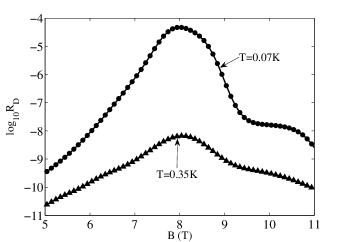
Figure 6: Drag resistance in the vortex paradigm at $T=0.07$K, with the metallic phase modeled as classical hard-disc liquid. Everything else is the same those in FIG. 2.

Putting these formulae together, we can compute the vortex density response function in (93) and insert it into the drag resistance formula (15). The drag resistance is shown in FIG. 6. One can see that it is remarkably close to our results obtained in Sec. (II.2), and thereby demonstrating that the scale of the drag resistance in the metallic regime is mainly set by the factors $dR/dB$ and is not sensitive to the statistics of the vortex particles.

Appendix E Coulomb Drag for disordered electron glass

In this section, we calculate the drag resistance due to Coulomb interaction between two disordered electron glasses with finite thickness. This calculation is related to the work of Ref. Shimshoni, 1997, but in our case the screening of the interlayer Coulomb interaction is important (see below), and we take into account the effect of finite film thickness.

The general formula for Coulomb drag resistance in $d$ dimensions isZheng and MacDonald (1993); Kamenev and Oreg (1995)

$$\rho_{D}^{ij}=\frac{\hbar^{2}}{e^{2}}\frac{1}{2\pi n^{2}T}\frac{1}{\Omega}\sum_{\vec{k}}k^{i}k^{j}\int_{0}^{\infty}\frac{\mathrm{d}\omega}{\sinh\frac{\hbar\omega}{2T}}|U|^{2}\operatorname{Im}\chi_{1}\operatorname{Im}\chi_{2}.$$ (110)

For the quasi-2d film we are considering, we can break the wavevector summation into two summations: one over $k_{z}$, another over the 2d wavevector $\vec{q}$. The $k_{z}$ summation is dominated by the term with $k_{z}=0$ component, which physically corresponds to the configuration with constant density along $z$-direction. In this case, we can use the quasi-2d form of the intralyer and interlayer Coulomb interaction potentials

$$U_{i}(\vec{q},k_{z}=0)=\frac{2\pi e^{2}d}{q},\qquad U_{e}(\vec{q},k_{z}=0)=\frac{2\pi e^{2}d}{q}e^{-qa},$$

where $d$ is the film thickness, and $a$ is the center-to-center layer separation. The real and imaginary parts of the density response function for a localized electron gas isVollhardt and Wolfle (1980, 1992); Imry et al. (1982)

$$\operatorname{Re}\chi(\vec{q},k_{z}=0,\omega) =\nu(q^{2}+k_{z}^{2})\xi^{2}\Big{|}_{k_{z}=0}=\nu q^{2}\xi^{2},$$

$$\operatorname{Im}\chi(\vec{q},k_{z}=0,\omega) =\nu\frac{(q^{2}+k_{z}^{2})\omega\xi^{4}}{D}\Big{|}_{k_{z}=0}=\nu\frac{q^{2}\omega\xi^{4}}{D},$$

where $\nu$ is the 3d density of states at the Fermi energy, and $\xi$ is the localization length, and $D$ is the diffusion constant in the conducting phase. The above expression is valid so long as $\operatorname{Im}\chi\ll\operatorname{Re}\chi$, which is straightforward to verify in our case recalling that $\omega$ is cut off by the temperature $T$ in (110).

Thus, in the screened interlayer interaction we can neglect $\operatorname{Im}\chi$ compared to $\operatorname{Re}\chi$:

$$U =\frac{U_{i}e^{-qa}}{(1+U_{i}\chi_{1})(1+U_{i}\chi_{2})-(U_{i}e^{-qa}\chi_{1})(U_{i}e^{-qa}\chi_{2})}$$

$$\approx\frac{1}{2U_{i}\operatorname{Re}\chi_{1}\operatorname{Re}\chi_{2}\sinh(qa)},$$ (111)

where in the last line we have made an approximation that $U_{i}\operatorname{Re}\chi\gg 1$, i.e.,

$$qa\gg x_{0}\equiv\frac{a}{\nu\xi^{2}2\pi e^{2}d}.$$ (112)

We have verified that the contribution from $0<qa<x_{0}$ is negligible compared to that from $qa>x_{0}$. Therefore,

$$R_{D} =\frac{\rho_{D}^{xx}}{d}$$

$$=\frac{1}{8\pi^{2}(nd)^{2}T}\frac{\hbar^{2}}{e^{2}}\int_{x_{0}}^{\infty}q^{3}\mathrm{d}q$$

$$\times\int_{0}^{\infty}\frac{\mathrm{d}\omega}{\sinh^{2}\frac{\hbar\omega}{2T}}\frac{\operatorname{Im}\chi_{1}\operatorname{Im}\chi_{2}}{4U_{i}^{2}(\operatorname{Re}\chi_{1})^{2}(\operatorname{Re}\chi_{2})^{2}\sinh^{2}(qa)}$$

$$=\frac{T^{2}}{128\pi^{4}\hbar e^{2}(nda)^{2}(D_{1}e^{2}d\nu)(D_{2}e^{2}d\nu)}$$

$$\times\int_{x_{0}}^{\infty}\frac{x\mathrm{d}x}{\sinh^{2}x}\int_{0}^{\infty}\frac{x^{2}\mathrm{d}x}{\sinh^{2}(x/2)}$$

$$=\frac{T^{2}}{128\pi^{4}\hbar e^{2}(nda)^{2}(D_{1}e^{2}d\nu)(D_{2}e^{2}d\nu)}\log\frac{1}{2x_{0}}\frac{4\pi^{2}}{3}$$

$$=\frac{T^{2}}{96\pi^{2}\hbar e^{2}(nda)^{2}(D_{1}e^{2}d\nu)(D_{2}e^{2}d\nu)}\log\frac{1}{2x_{0}}.$$

Note that

$$De^{2}d\nu=\frac{1}{R},$$ (113)

we have

$$R_{D} =\frac{T^{2}R_{1}R_{2}}{96\pi^{2}\hbar e^{2}(nda)^{2}}\log\frac{1}{2x_{0}}$$

$$=\frac{1}{96\pi^{2}}\frac{R_{1}R_{2}}{\hbar/e^{2}}\left(\frac{T}{e^{2}nda}\right)^{2}\log\frac{1}{2x_{0}}.$$ (114)

Since $D$ is the diffusion constant in the conducting phase, $R$ in the above expression should also be the resistance of the conducting phase. Thus this expression gives a slight overestimate of the drag resistance in the percolation paradigm if we use the value of $R_{NN}$ of the insulating phase for simplicity.

Note that our derivation relied on momentum summations. There are concerns that such an approach, although quite common in the literature, is incorrect when attempting to describe drag in strongly disordered systems. For our purposes, the derivation based on Eq. 110 is sufficient; this issue is taken up, however, in Ref. Apalkov and Raikh, 2005.

Appendix F The absence of measurable drag effect associated with a genuine superconductor in a resistor network

In this section, we show that a genuine superconducting link (i.e., without mobile vortices) has no measurable drag effect in a resistor network.

Figure 7: The typical setup for a drag effect experiment: in the active layer, a driving current $I_{1}$ flows through a resistor $R_{1}$ (normal or superconducting) with a voltage drop $V_{1}=I_{1}R_{1}$. In the passive layer, certain interaction effect takes place in a resistor $R_{2}$ (normal or superconducting), which may result in a drag current $I_{2}$ and a voltage drop $V_{2}$ across $R_{2}$. $R_{2}$ is also connected to another resistor $R_{0}$, which can be of any value.

FIG. 7 illustrates the typical setup for a drag effect experiment: in the active layer, a driving current $I_{1}$ flows through a resistor $R_{1}$ (normal or superconducting) with a voltage drop $V_{1}=I_{1}R_{1}$. In the passive layer, certain interaction effects take place in a resistor $R_{2}$ (normal or superconducting), which may result in a drag current $I_{2}$ and a voltage drop $V_{2}$ across $R_{2}$. $R_{2}$ is also connected to another resistor $R_{0}$, which might represent a voltmeter, an open circuit ($R_{0}=\infty$), or something else.

When one talks about the drag effect, there are two different concepts one needs to distinguish. The first one is the ”intrinsic” effect, which manifests itself by the appearance of a drag current $I_{D}$ in the passive layer if $R_{0}=0$. Generically, we have

$$I_{D}\equiv I_{2}|_{R_{0}=0}=\eta I_{1}.$$ (115)

For example, for the case of $R_{1},R_{2}>0$, i.e., both $R_{1}$ and $R_{2}$ are non-superconducting, $I_{2}|_{R_{0}=0}=\sigma_{D}V_{1}=\sigma_{D}I_{1}R_{1}$ (e.g., Coulomg drag between two 2DEGs), thus $\eta=\sigma_{D}R_{1}$; for $R_{1}=R_{2}=0$ (superconductor), we have the Cooper pair version of the supercurrent drag effect Eqn. (32), thus $\eta$ is finite in this case as well. For the case of $R_{1}>0$ (normal) and $R_{2}=0$ (superconducting), it would be unphysical to have $\eta=\infty$, thus we have $\eta<\infty$ and $\sigma_{D,NS}=\eta/R_{1}<\infty$. From Kubo formula for the drag conductance, we expect that $\sigma_{D,SN}=\sigma_{D,NS}<\infty$, and hence for the case of $R_{1}=0$ and $R_{2}>0$ we have $\eta=\sigma_{D,SN}R_{1}=0$.

In contrast, the second drag effect is the drag current $I_{2}$ in the presence of $R_{0}$, in which case he drag current at $R_{0}=0$ may or may not survive. In a large-size resistor network we are considering for the percolation picture, when we focus on the drag effect of one specific link $R_{2}$, we can simplify the circuit of the passive layer to be of the form in FIG. 7, in which case $R_{0}$ representing the rest of the circuit is almost always larger than $0$. If the drag effect survives the presence of the nonzero $R_{0}$, it will manifest itself as the appearance of a non-zero drag emf $\varepsilon_{D}$ on $R_{2}$. To see this, first consider the case $R_{2}>0$, and $R_{1}$ can be either $0$ or $>0$. $I_{2}$ receives contribution from both Ohm’s law and the drag effect:

$$I_{2}=\frac{V_{2}}{R_{2}}+\eta I_{1}=-\frac{I_{2}R_{0}}{R_{2}}+\eta I_{1},$$ (116)

thus

$$I_{2}=\frac{(\eta R_{2})I_{1}}{R_{0}+R_{2}}\equiv\frac{R_{D}I_{1}}{R_{0}+R_{2}}\equiv\frac{\varepsilon_{D}}{R_{0}+R_{2}},$$ (117)

where $\varepsilon_{D}=R_{D}I_{1}$ is the drag emf, and $R_{D}=\eta R_{2}$ is the drag resistance. If $R_{1}=0$ (superconducting) and $R_{2}>0$ (normal), we argued earlier that $\eta=0$, and thus $\varepsilon_{D}=R_{D}=0$ and there is no drag effect.

If $R_{2}=0$ (superconductor), no matter if $R_{1}=0$ (superconducting) or $>0$ (normal), it is straightforward to see from Kirchoff’s Law that we have only one steady-state solution $I_{2}|_{R_{0}>0}=0$. More insight into this case can be gained by considering what happens in real time. Suppose at time $t=0$, the drag effect takes place, a drag supercurrent $I_{2}(R_{0}=0)$ starts to flow in the circuit. But due to the presence of the normal resistor $R_{0}$, a voltage $I_{2}R_{0}$ now exist on the supercondutor, which will crank up the phase winding of the superconductor and degrade the drag supercurrent, until a steady state is reached where the total supercurrent is zero. Thus, we see that for the case $R_{2}=0$ and $R_{0}>0$, there is no observable drag effect, i.e., $I_{2}|_{R_{0}>0}=0$, $\varepsilon_{D}=I_{2}(R_{2}+R_{0})=0$, $R_{D}=\varepsilon_{D}/I_{1}=0$, although there is nonzero “intrinsic” drag effect $\eta$.

We can also understand this result $R_{D}=0$ for $R_{2}=0$ by examining the expression $R_{D}=\eta R_{2}$. For both the case of $R_{1}=R_{2}=0$ and the case of $R_{1}>0$ and $R_{2}=0$, we found earlier that $\eta<\infty$, and thus the drag resistance $R_{D}=\eta R_{2}$ and the drag emf $\varepsilon_{D}$ are $0$ for $R_{2}=0$.

In conclusion, we have shown that when connected with a nonzero resistor, as typically true in a resistor network, a genuine superconducting link has no measurable drag effect at all, no matter whether it is vertically aligned with a normal link or another superconducting link.

References

- Zou et al. (2009) Y. Zou, G. Refael, and J. Yoon, Phys. Rev. B 80, 180503 (2009).
- Sambandamurthy et al. (2004) G. Sambandamurthy, L. W. Engel, A. Johansson, and D. Shahar, Phys. Rev. Lett. 92, 107005 (2004).
- Fisher and Lee (1989) M. P. A. Fisher and D. H. Lee, Phys. Rev. B 39, 2756 (1989).
- Fisher (1990) M. P. A. Fisher, Phys. Rev. Lett. 65, 923 (1990).
- Wen and Zee (1990) X. G. Wen and A. Zee, Int. J. Mod. Phys. B 4, 437 (1990).
- Fisher et al. (1990) M. P. A. Fisher, G. Grinstein, and S. M. Girvin, Phys. Rev. Lett. 64, 587 (1990).
- Cha et al. (1991) M. C. Cha, M. P. A. Fisher, S. M. Girvin, M. Wallin, and A. P. Young, Phys. Rev. B 44, 6883 (1991).
- Wallin et al. (1994) M. Wallin, E. S. Sorensen, S. M. Girvin, and A. P. Young, Phys. Rev. B 49, 12115 (1994).
- Haviland et al. (1989) D. B. Haviland, Y. Liu, and A. M. Goldman, Phys. Rev. Lett. 62, 2180 (1989).
- Hebard and Paalanen (1990) A. F. Hebard and M. A. Paalanen, Phys. Rev. Lett. 65, 927 (1990).
- Paalanen et al. (1992) M. A. Paalanen, A. F. Hebard, and R. R. Ruel, Phys. Rev. Lett. 69, 1604 (1992).
- Valles et al. (1992) J. M. Valles, R. C. Dynes, and J. P. Garno, Phys. Rev. Lett. 69, 3567 (1992).
- Liu et al. (1993) Y. Liu, D. B. Haviland, B. Nease, and A. M. Goldman, Phys. Rev. B 47, 5931 (1993).
- Hsu et al. (1995) S. Y. Hsu, J. A. Chervenak, and J. M. Valles, Phys. Rev. Lett. 75, 132 (1995).
- Valles et al. (1994) J. M. Valles, S. Y. Hsu, R. C. Dynes, and J. P. Garno, Physica B 197, 522 (1994).
- Yazdani and Kapitulnik (1995) A. Yazdani and A. Kapitulnik, Phys. Rev. Lett. 74, 3037 (1995).
- Hsu et al. (1998) S. Y. Hsu, J. A. Chervenak, and J. M. Valles, J. Phys. Chem. Solids 59, 2065 (1998).
- Goldman and Markovic (1998) A. M. Goldman and N. Markovic, Phys. Today 51, 39 (1998).
- (19) M. A. Steiner, N. P. Breznay, and A. Kapitulnik, arxiv.org/abs/0710.1822.
- Ephron et al. (1996) D. Ephron, A. Yazdani, A. Kapitulnik, and M. R. Beasley, Phys. Rev. Lett. 76, 1529 (1996).
- Mason and Kapitulnik (1999) N. Mason and A. Kapitulnik, Phys. Rev. Lett. 82, 5341 (1999).
- Mason and Kapitulnik (2001) N. Mason and A. Kapitulnik, Phys. Rev. B 64, 060504(R) (2001).
- Steiner and Kapitulnik (2005) M. A. Steiner and A. Kapitulnik, Physica C 422, 16 (2005).
- Seo et al. (2006) Y. Seo, Y. Qin, C. L. Vicente, K. S. Choi, and J. Yoon, Phys. Rev. Lett. 97, 057005 (2006).
- Qin et al. (2006) Y. Qin, C. L. Vicente, and J. Yoon, Phys. Rev. B 73, 100505(R) (2006).
- Li et al. (2010) Y. Li, C. L. Vicente, and J. Yoon, Phys. Rev. B 81, 020505 (2010).
- Baturina et al. (2004) T. I. Baturina, D. R. Islamov, J. Bentner, C. Strunk, M. R. Baklanov, and A. Satta, JETP Lett. 79, 337 (2004).
- Gantmakher and Dolgopolov (2010) V. Gantmakher and V. Dolgopolov, Physics-Uspekhi 53, 3 (2010).
- Feigelman et al. (1993) M. V. Feigelman, V. B. Geshkenbein, L. B. Ioffe, and A. I. Larkin, Phys. Rev. B 48, 16641 (1993).
- Balents and Fisher (2005) L. Balents and M. P. A. Fisher, Phys. Rev. B 71, 085119 (2005).
- Galitski et al. (2005) V. M. Galitski, G. Refael, M. P. A. Fisher, and T. Senthil, Phys. Rev. Lett. 95, 077002 (2005).
- Shimshoni et al. (1998) E. Shimshoni, A. Auerbach, and A. Kapitulnik, Phys. Rev. Lett. 80, 3352 (1998).
- Ghosal et al. (2001) A. Ghosal, M. Randeria, and N. Trivedi, Phys. Rev. B 65, 014501 (2001).
- Dubi et al. (2006) Y. Dubi, Y. Meir, and Y. Avishai, Phys. Rev. B 73, 054509 (2006).
- Dubi et al. (2007) Y. Dubi, Y. Meir, and Y. Avishai, Nature 449, 876 (2007).
- Spivak et al. (2008) B. Spivak, P. Oreto, and S. A. Kivelson, Phys. Rev. B 77, 214523 (2008).
- Dalidovich and Phillips (2002) D. Dalidovich and P. Phillips, Phys. Rev. Lett. 89, 027001 (2002).
- Wu and Phillips (2006) J. Wu and P. Phillips, Phys. Rev. B 73, 214507 (2006).
- Ikeda (2007) R. Ikeda, J. Phys. Soc. Jpn. 76, 064709 (2007).
- (40) A. Johansson, N. Stander, E. Peled, G. Sambandamurthy, and D. Shahar, arXiv:cond-mat/0602160.
- Crane et al. (2007) R. Crane, N. P. Armitage, A. Johansson, G. Sambandamurthy, D. Shahar, and G. Gruner, Phys. Rev. B 75, 184530 (2007).
- Spathis et al. (2008) P. Spathis, H. Aubin, A. Pourret, and K. Behnia, Europhys. Lett. 83, 57005 (2008).
- Sacepe et al. (2008) B. Sacepe, C. Chapelier, T. I. Baturina, V. M. Vinokur, M. R. Baklanov, and M. Sanquer, Phys. Rev. Lett. 101, 157006 (2008).
- Giaever (1965) I. Giaever, Phys. Rev. Lett. 15, 825 (1965).
- Michaeli and Finkel’stein (2006) K. Michaeli and A. M. Finkel’stein, Phys. Rev. Lett. 97, 117004 (2006).
- Mason and Kapitulnik (2002) N. Mason and A. Kapitulnik, Phys. Rev. B 65, 220505 (2002).
- Gramila et al. (1991) T. J. Gramila, J. P. Eisenstein, A. H. MacDonald, L. N. Pfeiffer, and K. W. West, Phys. Rev. Lett. 66, 1216 (1991).
- Pearl (1964) J. Pearl, Appl. Phys. Lett. 5, 65 (1964).
- De Col et al. (2005) A. De Col, V. B. Geshkenbein, and G. Blatter, Phys. Rev. Lett. 94, 097001 (2005).
- Sherrill (1973) M. D. Sherrill, Phys. Rev. B 7, 1908 (1973).
- Sherrill (1975) M. D. Sherrill, Phys. Rev. B 11, 1066 (1975).
- Jauho and Smith (1993) A.-P. Jauho and H. Smith, Phys. Rev. B 47, 4420 (1993).
- Zheng and MacDonald (1993) L. Zheng and A. H. MacDonald, Phys. Rev. B 48, 8203 (1993).
- Kamenev and Oreg (1995) A. Kamenev and Y. Oreg, Phys. Rev. B 52, 7516 (1995).
- Flensberg et al. (1995) K. Flensberg, B. Hu, A. Jauho, and J. M. Kinaret, Phys. Rev. B 52, 14761 (1995).
- von Oppen et al. (2001) F. von Oppen, S. H. Simon, and A. Stern, Phys. Rev. Lett. 87, 106803 (2001).
- Hwang et al. (2003) E. H. Hwang, S. D. Sarma, V. Braude, and A. Stern, Phys. Rev. Lett. 90, 086801 (2003).
- Leutheusser (1982) E. Leutheusser, J. Phys. C. 15, 2801 (1982).
- Leutheusser et al. (1983) E. Leutheusser, S. Yip, B. J. Alder, and W. E. Alley, J. Stat. Phys. 32 (1983).
- Mahan (1981) G. D. Mahan, Many-Particle Physics (Plenum Press, New York, 1981).
- Stern (1967) F. Stern, Phys. Rev. Lett. 18, 546 (1967).
- Duan and Yip (1993) J. M. Duan and S. Yip, Phys. Rev. Lett. 70, 3647 (1993).
- Terenttjev and Shevchenko (1999) S. V. Terenttjev and S. I. Shevchenko, Low Temp. Phys. 25, 493 (1999).
- Fil and Shevchenko (2004) D. V. Fil and S. I. Shevchenko, Low Temp. Phys. 30, 770 (2004).
- Narayan (2003) O. Narayan, J. Phys. A 36, L373 (2003).
- Kuprianov and Likharev (1975) Kuprianov and Likharev, Sov. Phys. JETP 41, 755 (1975).
- Blatter et al. (1991) G. Blatter, V. B. Geshkenbein, and V. M. Vinokur, Phys. Rev. Lett. 66, 3297 (1991).
- Duan and Leggett (1992) J.-M. Duan and A. J. Leggett, Phys. Rev. Lett. 68, 1216 (1992).
- Sonin et al. (1998) E. B. Sonin, V. B. Geshkenbein, A. van Otterlo, and G. Blatter, Phys. Rev. B 57, 575 (1998).
- Forster (1995) D. Forster, Hydrodynamic Fluctuations, Broken Symmetry, And Correlation Functions (Westview Press, 1995).
- Chaikin and Lubensky (1995) P. M. Chaikin and T. C. Lubensky, Principles of condensed matter physics (Cambridge University Press, 1995).
- Leutheusser (1986) E. Leutheusser, J. Chem. Phys. 84, 1050 (1986).
- Whitlock et al. (2007) P. A. Whitlock, M. Bishop, and J. L. Tiglias, J. Chem. Phys. 126, 224505 (2007).
- Shimshoni (1997) E. Shimshoni, Phys. Rev. B 56, 13301 (1997).
- Vollhardt and Wolfle (1980) D. Vollhardt and P. Wolfle, Phys. Rev. B 22, 4666 (1980).
- Vollhardt and Wolfle (1992) D. Vollhardt and P. Wolfle, in Electronic Phase Transitions, edited by W. Hanke and Y. V. Kopaev (North-Holland, 1992).
- Imry et al. (1982) Y. Imry, Y. Gefen, and D. J. Bergman, Phys. Rev. B 26, 3436 (1982).
- Apalkov and Raikh (2005) V. M. Apalkov and M. E. Raikh, Phys. Rev. B 71, 245109 (2005).