A simplified particulate model for coarse-grained hemodynamics simulations

Abstract

Human blood flow is a multi-scale problem: in first approximation, blood is a dense suspension of plasma and deformable red cells. Physiological vessel diameters range from about one to thousands of cell radii. Current computational models either involve a homogeneous fluid and cannot track particulate effects or describe a relatively small number of cells with high resolution, but are incapable to reach relevant time and length scales. Our approach is to simplify much further than existing particulate models. We combine well established methods from other areas of physics in order to find the essential ingredients for a minimalist description that still recovers hemorheology. These ingredients are a lattice Boltzmann method describing rigid particle suspensions to account for hydrodynamic long range interactions and—in order to describe the more complex short-range behavior of cells—anisotropic model potentials known from molecular dynamics simulations. Paying detailedness, we achieve an efficient and scalable implementation which is crucial for our ultimate goal: establishing a link between the collective behavior of millions of cells and the macroscopic properties of blood in realistic flow situations. In this paper we present our model and demonstrate its applicability to conditions typical for the microvasculature.

I Introduction

Human blood is not a homogeneous substance but can be approximated as a suspension of deformable red blood cells (RBCs, also called erythrocytes) in a Newtonian liquid, the blood plasma. Under physiological conditions the volume concentration of RBCs typically amounts to $40\,\%$ to $50\,\%$ in larger blood vessels. We neglect the other constituents like leukocytes and thrombocytes in this work due to their far lower volume concentrations Goldsmith and Skalak (1975). In the absence of external stresses, erythrocytes assume the shape of biconcave discs with a diameter of approximately $8\,\mu\text{m}$ Evans and Fung (1972). Their main biological task is the transport of oxygen in the body, but due to the high volume fraction they also strongly affect the rheology of blood and its clotting behavior Fung (1981). An understanding of these effects is necessary in order to study and to cure pathologically deviating phenomena in the body and to design microfluidic devices for improved blood analysis. In both cases, blood often has to be studied within complex geometries that elude an analytical description. However, also the computational treatment of blood is demanding. On large scales like in arteries with diameters in the order of millimeters, blood can be modeled as a continuous and even Newtonian fluid Boyd et al. (2007). Even then, the computational effort and the complexity of the model can be significant if realistic geometries show features which stretch over different length scales.

For modeling flow in the microvascular network, there is need for a description that accounts for the presence of discrete cells Popel and Johnson (2005). Recently, models of deformable cells were presented amongst others by Dupin et al. Dupin et al. (2008), in the group of Gompper McWhirter et al. (2009), and by Wu and Aidun Wu and Aidun (2010). Here, the cell membrane is simplified to a deformable mesh and coupled to a mesoscopic simulation method for the plasma like multi-particle collision dynamics McWhirter et al. (2009) or lattice Boltzmann (LB) Dupin et al. (2008); Wu and Aidun (2010). However, mainly because of the high resolution that is necessary for the elaborate description of the cells, these models are computationally too demanding for the application to considerably larger 3D systems.

Our motivation is to bridge the scales that are accessible with both classes of existing models by an intermediate approach: we keep the particulate nature of blood, but try to find a minimal description of each single cell. We thus deliberately simplify much further than the authors of the particulate models cited above in order to gain the potential for a computationally efficient and scalable implementation. Resorting to well-established methods from other areas of physics we explore the ingredients necessary to recover the rheological behavior of blood. It is not our motivation to account for sub-cell effects in more than a coarse-grained way. In this work we aim at the description and validation of such a model while presenting possible applications in the range from approximately $10\,\mu\text{m}$ upward. Our ultimate goal is to develop a quantitative method that allows to study the flow in realistic geometries but also to link bulk properties, for example the apparent viscosity, to phenomena at the level of single erythrocytes. In the case of cell deformation and aggregation in plane shear flow, this link has been established already in experiment and theory Chien (1970). Numerical simulations enable us to extend this knowledge to the case of arbitrary geometries and time-dependent flows. Further microscopic properties of interest are the alignment of cells or local changes of the cell concentration. The improved understanding of the dynamic behavior of blood might be used for the optimization of macroscopic simulation methods. Only a computationally efficient description allows the accumulation of firm statistical data that is necessary for this task.

The main idea of our model is to distinguish between the long-range hydrodynamic coupling of cells and the short-range interactions that are related to the complex mechanics, electrostatics, and the chemistry of the membranes. Long-range hydrodynamic interactions are considered by means of the LB method Succi (2001). This mesoscopic simulation method allows a relatively easy implementation of complex boundary conditions which are needed for the simulation of realistic geometries. Moreover, an efficient parallelization is straightforward which even with our simplified model is crucial for the accumulation of statistically relevant data or for the description of realistic systems like branching vessels. Research on a parallel and efficient implementation of the LB method for the simulation of flow in sparse vessel networks was published by various authors Axner et al. (2008); Mazzeo and Coveney (2008); Bernaschi et al. (2009). Consequently, the LB method was applied to blood flow already in earlier works though they differ from our approach in the accuracy with which cells are resolved. For example, Boyd et al. Boyd et al. (2007) model blood either as a Newtonian fluid or a homogeneous fluid with a shear rate-dependent viscosity. Further, the studies by Dupin et al. Dupin et al. (2008), Wu and Aidun Wu and Aidun (2010), Migliorini et al. Migliorini et al. (2002), and by Sun and Munn Sun and Munn (2006) involve LB solvers, but describe each RBC as either deformable or equipped with an elaborate cell adhesion model.

In contrast to those, we are interested in a minimal resolution of RBCs since reducing the resolution generally is the most effective way to enhance the efficiency of a fluid dynamics solver. Ahlrichs and Dünweg implement a dissipative coupling of point-particles to an LB fluid Ahlrichs and Dünweg (1998). However, the description of RBCs as point particles would involve a resolution which is so low that hydrodynamics in the smallest vessels becomes inaccessible. Concerning hydrodynamics, it is questionable whether the resolution of cell deformation has a benefit compared to a rigid particle model if each RBC is resolved with only a few lattice spacings. In consequence we decide for a method for suspensions of rigid particles of finite size that is similar to the one described in Aidun et al. (1998). As will be explained below, not volume-conserving cell deformations of the order of one lattice spacing occur as an artefact of the method already but do not show significant influence on the flow behavior. Ding and Aidun simulated rigid particles with the biconcave shape of unstressed red blood cells using an LB method Ding and Aidun (2006). It is known, however, that RBCs abandon this equilibrium shape and instead resemble elongated ellipsoids when exposed to shear flow Fischer et al. (1978). Thus, taking into account the limited lattice resolution, we decide for discretized ellipsoidal model cells with rotational symmetry as an approximation of the shapes actually assumed by real erythrocytes in many flow situations. Differently from Nguyen and Ladd (2002); Ding and Aidun (2003, 2006), our implementation does not enforce rigid particle surfaces since this would be in contradiction with the nature of deformable erythrocytes. Especially in bulk flow at high volume concentrations but also in capillaries due to the influence of walls, the flow is not dominated by long-range hydrodynamics but by short-range cell-cell and cell-wall effects. Thus, a coarse-grained description using effective cell and wall interactions is appropriate. We account for the complex short-range behavior of RBCs on a phenomenological level by means of model potentials. Our potentials serve to provide a softly repulsive core that follows the approximated ellipsoidal RBC shape. For this purpose, the method of Berne and Pechukas Berne and Pechukas (1972) is applied in order to anisotropically rescale a Hookian spring potential.

In the following section II we provide an introduction to the application of the LB method to suspensions of rigid particles and discuss how our model differs from other implementations. In section III we develop phenomenological potentials for the anisotropic interaction of two cells and of cells and walls. Section IV opens with the search for a parametrization which fits to experimental literature data. This set of parameters is then used to demonstrate the applicability of the new model to confined systems. We further discuss the performance of our implementation for large systems and conclude with a summary in section V.

II Hydrodynamic part of the model

To model the blood plasma that surrounds the cells the LB method is applied. For a comprehensive introduction we refer to Succi (2001). The fluid traveling with one of $r$ discrete velocities $\mathbf{c}_{r}$ at the three-dimensional lattice position $\mathbf{x}$ and discrete time $t$ is resembled by the single particle distribution function $n_{r}(\mathbf{x},t)$. Its evolution in time is determined by collision

$$n^{*}_{r}(\mathbf{x},t)=n_{r}(\mathbf{x},t)-\Omega$$ (1)

and the successive advection

$$n_{r}(\mathbf{x}+\mathbf{c}_{r},t+1)=n^{*}_{r}(\mathbf{x},t)$$ (2)

of the post-collision distribution $n^{*}_{r}(\mathbf{x},t)$. Eq. 1 and Eq. 2 together can be written as the lattice Boltzmann equation

$$n_{r}(\mathbf{x}+\mathbf{c}_{r},t+1)=n_{r}(\mathbf{x},t)-\Omega\text{ .}$$ (3)

For the sake of simplicity and computational efficiency we follow a D3Q19 approach with a single relaxation time $\tau$ Qian et al. (1992). We thus have $19$ discrete velocities and the BGK-collision term Bhatnagar et al. (1954)

$$\Omega=\frac{n_{r}(\mathbf{x},t)-n_{r}^{\text{eq}}(\rho(\mathbf{x},t),\mathbf{u}(\mathbf{x},t))}{\tau},$$ (4)

where the equilibrium distribution function

$$n_{r}^{\text{eq}}(\rho,\mathbf{u}) = \rho\alpha_{c_{r}}\Bigg{[}1+\frac{\mathbf{c}_{r}\mathbf{u}}{c_{\text{s}}^{2}}+\frac{\left(\mathbf{c}_{r}\mathbf{u}\right)^{2}}{2c_{\text{s}}^{4}}-\frac{\mathbf{u}^{2}}{2c_{\text{s}}^{2}}$$ (5)

$${}+\frac{\left(\mathbf{c}_{r}\mathbf{u}\right)^{3}}{6c_{\text{s}}^{6}}-\frac{\mathbf{u}^{2}\mathbf{c}_{r}\mathbf{u}}{2c_{\text{s}}^{4}}\Bigg{]}$$

is an expansion of the Maxwell-Boltzmann distribution of third order in velocity $\mathbf{u}$ Chen et al. (2000). The value of the speed of sound $c_{\text{s}}=1/\sqrt{3}$ depends on the choice of the lattice. The same holds for the lattice weights

$$\alpha_{c_{r}}=\left\{\begin{array}[]{l@{\quad\text{for }c_r=\,\,}l}1/3\hfil\quad\text{for }c_&0\\ 1/18\hfil\quad\text{for }c_&1\\ 1/36\hfil\quad\text{for }c_&\sqrt{2}\end{array}\right.\text{ ,}$$ (6)

which differ for lattice velocities $\mathbf{c}_{r}$ according to their absolute value $c_{r}$. The local density

$$\rho(\mathbf{x},t)=\sum_{r}n_{r}(\mathbf{x},t)$$ (7)

and velocity

$$\mathbf{u}(\mathbf{x},t)=\frac{\sum_{r}n_{r}(\mathbf{x},t)\mathbf{c}_{r}}{\rho(\mathbf{x},t)}$$ (8)

are calculated as moments of the fluid distribution with respect to the set of discrete velocities. Both are invariants of the BGK collision rule Eq. 1. This method is well established for the simulation of the liquid phase of suspensions Aidun et al. (1998); Nguyen and Ladd (2002), namely blood Dupin et al. (2008); Wu and Aidun (2010). It can be shown that in the limit of small velocities and lattice spacings the Navier-Stokes equations are recovered with a kinematic viscosity $\nu=(2\tau-1)/6$.

For a coarse-grained description of the hydrodynamic interaction of cells and blood plasma, a method similar to the ones explained in Aidun et al. (1998) and Nguyen and Ladd (2002) modeling rigid particles of finite size is applied. Starting point is the mid-link bounce-back boundary condition that implements no-slip boundaries for the fluid: arbitrarily shaped geometries are discretized on the lattice by turning the lattice nodes on the solid side of the theoretical solid-fluid interface into fluid-less wall nodes. If $\mathbf{x}$ is such a node the updated distribution at $\mathbf{x}+\mathbf{c}_{r}$ is not determined by the advection rule Eq. 2 but according to

$$n_{r}(\mathbf{x}+\mathbf{c}_{r},t+1)=n^{*}_{\bar{r}}(\mathbf{x}+\mathbf{c}_{r},t)$$ (9)

which means replacing the local distribution with the post-collision distribution of the opposite direction $\bar{r}$ (defined by $\mathbf{c}_{\bar{r}}\equiv-\mathbf{c}_{r}$). We make use of this boundary condition to implement (rigid) vessel walls.

To model boundaries moving with velocity $\mathbf{v}$, Eq. 9 can be complemented with a correction term

$$C=\frac{2\alpha_{c_{r}}}{c_{\text{s}}^{2}}\rho(\mathbf{x}+\mathbf{c}_{r},t)\,\mathbf{c}_{r}\mathbf{v}$$ (10)

which is of first order in velocity. Inserting Eq. 5 and Eq. 10, one can easily prove that the new update rule

$$n_{r}(\mathbf{x}+\mathbf{c}_{r},t+1)=n^{*}_{\bar{r}}(\mathbf{x}+\mathbf{c}_{r},t)+C$$ (11)

is up to second order consistent with the equilibrium distribution function Eq. 5 for the general case $\mathbf{u}=\mathbf{v}\not=\mathbf{0}$.

When used to implement freely moving particles, it is necessary to keep track of the momentum

$$\Delta\mathbf{p}_{\text{fp}}=\left(2n_{\bar{r}}+C\right)\mathbf{c}_{\bar{r}}\text{ ,}$$ (12)

which is transferred during each time step by each single bounce-back process. According to the choice of unit time steps it is equal to the resulting force on the particle. The equations of motion of the particles are integrated like in classical molecular dynamics (MD) simulations to achieve the time evolution of the system. We implement a combined LB/MD code in which both the time step and the spatial decomposition scheme are shared between the two methods. A leap-frog integrator that is adapted to the internal representation of the cell orientations based on unit quaternions is applied Allen and Tildesley (1991).

Due to discretization errors the representation of a particle on the lattice slightly changes its shape and volume during movement. When new lattice sites are covered, the fluid at those is deleted. When a site formerly occupied by a particle is freed, new fluid is created according to Eq. 5. In doing so, the initial density $\bar{\rho}$ of the simulation is utilized as $\rho$. The velocity $\mathbf{u}$ is estimated according to the translational and rotational velocity of the particle and the no-slip assumption. In both cases the change in total fluid momentum is balanced by an additional force on the respective particle.

Physiological RBCs, however, are deformable and assume the shape of biconcave discs in the absence of external stresses Evans and Fung (1972). Despite the coarse-graining in our model, we do not want to give up the anisotropy of RBCs. Obviously, anisotropic model cells are able to display a much richer behavior than radially symmetric particles. We thus choose a simplified ellipsoidal geometry that is defined by two distinct half-axes $R_{\parallel}$ and $R_{\perp}$ parallel and perpendicular to the unit vector $\hat{\mathbf{o}}_{i}$ which points along the direction of the axis of rotational symmetry of each particle $i$.

Closely approaching particles are modeled as follows: when there are still fluid nodes between both discretized volumes the LB method is able to keep track of the emerging lubrication forces apart from discretization errors. As soon as there is a direct particle-particle interface without intermediate fluid nodes, the lubrication forces cannot be covered by a lattice-based method anymore. Moreover, an effective attraction becomes visible because of the missing fluid pressure in between the particles. Typical applications of this simulation method to the case of dense suspensions additionally feature analytical short-range lubrication corrections to overcome this problem Ding and Aidun (2003); Nguyen and Ladd (2002). These are implemented as pair-forces that depend on the relative velocity and diverge for vanishing gap-widths. However, this procedure is inappropriate for a model for suspensions of deformable cells. Since the theoretical particle shapes defined by $R_{\parallel}$ and $R_{\perp}$ are fixed, our application even requires tolerance for the overlap of the discretized volumes in order to account for the case where two cells strongly deform while approaching each other. Due to the complexity of the emerging forces that include electrostatic repulsion and van der Waals forces but also the mechanics and chemistry of the cell membranes and the rheology of the cell plasma, we cover them on a purely phenomenological level in the next section. Here, we support the LB method with additional rules which result in forces for the case of two particles in direct contact with each other that are neither divergent nor excessively attractive. Wherever a direct particle-particle interface is encountered, we apply a pair of mutual forces

$$\mathbf{F}_{\text{pp}}^{+}=2n_{r}^{\text{eq}}(\bar{\rho},\mathbf{u}=\mathbf{0})\mathbf{c}_{r}$$ (13)

and

$$\mathbf{F}_{\text{pp}}^{-}=2n_{\bar{r}}^{\text{eq}}(\bar{\rho},\mathbf{u}=\mathbf{0})\mathbf{c}_{\bar{r}}=-\mathbf{F}_{\text{pp}}^{+}$$ (14)

at each link across the interface which are directed towards each respective particle. Comparison with Eq. 12 shows that this is exactly the momentum transfer during one time step due to the rigid-particle algorithm for a resting particle and an adjacent site with resting fluid at equilibrium and initial density $\bar{\rho}$. The fluid in our simulation is to good approximation incompressible and the velocities are small. The forces arising from those regions of the particle surfaces that are in contact with the fluid therefore are largely compensated and do not cause an artificial attraction. In consequence, the self-induced collapse of particles in contact is prevented without the need for divergent lubrication corrections as in rigid-particle models. Moreover, for a given system, Eq. 13 and Eq. 14 depend only on $\mathbf{c}_{r}=-\mathbf{c}_{\bar{r}}$. For symmetry reasons, $n_{r}^{\text{eq}}(\bar{\rho},\mathbf{0})=n_{\bar{r}}^{\text{eq}}(\bar{\rho},\mathbf{0})$ holds. Thus, the momentum balance is kept since the two forces emerging from any particle-particle link compensate each other. However, since Eq. 13 and Eq. 14 do not depend on the relative velocity they cannot cover dissipative forces between particles. This limitation needs to be kept in mind when deciding about phenomenological cell-cell forces and their parametrization later in this paper.

For the sake of simplicity we do not allow a lattice node to be occupied by more than one cell. Occupation instead is determined by the order in which cells arrive at a node. From the point of view of the surrounding fluid this behavior is physically consistent with two particles that compressibly deform upon contact. The compressibility, however, can lead to an artificial increase of the total mass since the number of fluid nodes increases temporarily and we do not adjust the particle mass dynamically according to the volume occupied momentarily. Thus, in an ensemble of many cells, there are fluctuations of the total mass due to the introduction of the correction term $C$ in Eq. 11 and due to the change in total volume of the solid phase which fluctuates when cells move and increases when they overlap. However, even during millions of time steps we find no drift of the total mass for the systems we simulate here.

In case of close contact of cells with the confining geometry we proceed in a similar manner as for two cells. The only difference is that the forces on the system walls are ignored since they are assumed to be rigid and fixed.

III Model potentials for cell-cell and cell-wall interactions

In order to account for the complex behavior of real RBCs at small distances we add phenomenological pair potentials. For simplicity, we restrict ourselves to repulsive forces. This can be justified because in many physiological situations of interest, for example close to the walls of large parts of the arterial system, high shear rates render aggregative effects negligible Stroev et al. (2007); Chien (1970). The task of the potential therefore lies in establishing an excluded volume for each cell. Due to the mild increase of the potential, an overlap of these volumes will be unfavorable yet possible to some degree. Thus, the deformation of cells upon contact is modeled in a phenomenological way. A simplified potential also is beneficial to the efficiency of the model since it can be evaluated with less numerical effort and is less likely to demand small time steps or high order integrators. We start with the repulsive branch of a Hookian spring potential

$$\phi(r_{ij})=\left\{\begin{array}[]{l@{\qquad}l}\varepsilon\left(1-r_{ij}/\sigma\right)^{2}&r_{ij}<\sigma\\ 0&r_{ij}\geq\sigma\end{array}\right.$$ (15)

for the scalar displacement $r_{ij}$ of two particles $i$ and $j$. This is probably the simplest way to describe (elastic) deformability. The energy at zero displacement and the distance at which the repulsive potential force sets in can be directly controlled by means of the parameters $\varepsilon$ and $\sigma$. With respect to the disc-like shape of RBCs, we follow the approach of Berne and Pechukas Berne and Pechukas (1972) and choose the stiffness parameter

$$\varepsilon(\hat{\mathbf{o}}_{i},\hat{\mathbf{o}}_{j})=\frac{\bar{\varepsilon}}{\sqrt{1-\chi^{2}\left(\hat{\mathbf{o}}_{i}\hat{\mathbf{o}}_{j}\right)^{2}}}$$ (16)

and the size parameter

$$\sigma(\hat{\mathbf{o}}_{i},\hat{\mathbf{o}}_{j},\hat{\mathbf{r}}_{ij})=\frac{\bar{\sigma}}{\sqrt{1-\frac{\chi}{2}\left[\frac{\left(\hat{\mathbf{r}}_{ij}\hat{\mathbf{o}}_{i}+\hat{\mathbf{r}}_{ij}\hat{\mathbf{o}}_{j}\right)^{2}}{1+\chi\hat{\mathbf{o}}_{i}\hat{\mathbf{o}}_{j}}+\frac{\left(\hat{\mathbf{r}}_{ij}\hat{\mathbf{o}}_{i}-\hat{\mathbf{r}}_{ij}\hat{\mathbf{o}}_{j}\right)^{2}}{1-\chi\hat{\mathbf{o}}_{i}\hat{\mathbf{o}}_{j}}\right]}}$$ (17)

as functions of the orientations $\hat{\mathbf{o}}_{i}$ and $\hat{\mathbf{o}}_{j}$ of the cells and their normalized center displacement $\hat{\mathbf{r}}_{ij}$. We achieve an anisotropic potential with a zero-energy surface that is approximately that of ellipsoidal discs. Their half-axes $\sigma_{\parallel}$ and $\sigma_{\perp}$ parallel and perpendicular to the symmetry axis enter Eq. 16 and Eq. 17 via

$$\bar{\sigma}=2\sigma_{\perp}\quad\text{and}\quad\chi=\frac{\sigma_{\parallel}^{2}-\sigma_{\perp}^{2}}{\sigma_{\parallel}^{2}+\sigma_{\perp}^{2}}\text{ ,}$$ (18)

whereas $\bar{\varepsilon}$ determines the potential strength. The above approach for anisotropic rescaling of radial symmetric potentials and its later improvement by Gay and Berne Gay and Berne (1981) were intended for modeling liquid crystal systems. Particularly the method by Gay and Berne is applied almost exclusively to a Lennard-Jones potential featuring a short range repulsion and an attraction on moderate distances. This is referred to as “Gay-Berne potential” in the literature. The model potential presented by us lacks the attractive tail but is equipped only with a softly repulsive core. In consequence, there is no force acting on particles separated by more than the respective core diameter and at physiological volume concentrations we cannot expect to observe spontaneous ordering of the system. Compared to typical liquid crystal applications, the role of our potential lies rather in providing a soft repulsion within an anisotropic discoid volume than in making specific cell alignments more favorable compared to others. Fig. 1 displays in dimensionless form the magnitude of the resultant repulsive pair force $F$ as a function of $r_{ij}$ for $\sigma_{\perp}=3\sigma_{\parallel}$ and three simple sets of relative orientations: $\hat{\mathbf{o}}_{i}\parallel\hat{\mathbf{o}}_{j}\perp\hat{\mathbf{r}}_{ij}$, $\hat{\mathbf{o}}_{i}\parallel\hat{\mathbf{o}}_{j}\parallel\hat{\mathbf{r}}_{ij}$, and $\hat{\mathbf{o}}_{i}\perp\hat{\mathbf{o}}_{j}\parallel\hat{\mathbf{r}}_{ij}$. Depending on the orientations, the repulsive force sets in at different $r_{ij}$. Aiming at the presentation of a model potential which is simplified to the greatest possible extent, we chose the Berne-Pechukas approach which is slightly less complex than the more popular one by Gay and Berne. In this approach, it is not possible to independently adjust the interaction strength for different molecular orientations. That the potential is considerably stiffer in the case where the flat sides of both cells are aligned towards each other is, however, consistent with the fact that for this orientation, the same linear approach creates a significantly larger overlap volume than in the other two cases. In the following section, we will find values for $\bar{\varepsilon}$, $\sigma_{\parallel}$, and $\sigma_{\perp}$ that reproduce the rheological behavior of blood.

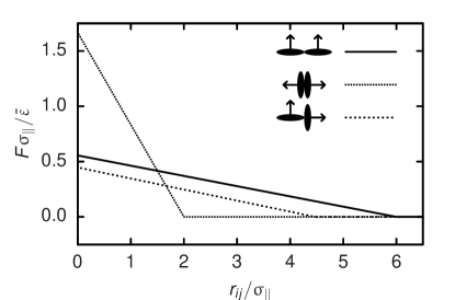
Figure 1: Dimensionless repulsive potential force as a function of the dimensionless center distance for $\sigma_{\perp}=3\sigma_{\parallel}$ and three sets of relative orientations $\hat{\mathbf{o}}_{i}\parallel\hat{\mathbf{o}}_{j}\perp\hat{\mathbf{r}}_{ij}$, $\hat{\mathbf{o}}_{i}\parallel\hat{\mathbf{o}}_{j}\parallel\hat{\mathbf{r}}_{ij}$, and $\hat{\mathbf{o}}_{i}\perp\hat{\mathbf{o}}_{j}\parallel\hat{\mathbf{r}}_{ij}$. An approximately ellipsoidal excluded volume can be deducted from the surface at which the repulsion sets in.

For modeling the cell-wall interaction we assume a sphere with radius $\sigma_{\text{w}}=1/2$ at every lattice node on the surface of a vessel wall and implement similar potential forces as for the cell-cell interaction based on the repulsive spring potential Eq. 15. Berne and Pechukas show that using

$$\sigma(\hat{\mathbf{o}}_{i},\hat{\mathbf{r}}_{i\mathbf{x}})=\frac{\bar{\sigma}_{\text{w}}}{\sqrt{1-\chi_{\text{w}}\left(\hat{\mathbf{r}}_{i\mathbf{x}}\hat{\mathbf{o}}_{i}\right)^{2}}}$$ (19)

instead of Eq. 17 as a size parameter with

$$\bar{\sigma}_{\text{w}}=\sqrt{\sigma_{\perp}^{2}+\sigma_{\text{w}}^{2}}\qquad\text{and}\qquad\chi_{\text{w}}=\frac{\sigma_{\parallel}^{2}-\sigma_{\perp}^{2}}{\sigma_{\parallel}^{2}+\sigma_{\text{w}}^{2}}$$ (20)

allows to scale a potential with radial symmetry to fit for the description of the interaction of a sphere and an ellipsoidal disc Berne and Pechukas (1972). $\hat{\mathbf{r}}_{i\mathbf{x}}$ is the normalized center displacement of particle $i$ and a wall node $\mathbf{x}$. It is not necessary to scale the stiffness parameter anisotropically, instead we set $\varepsilon(\hat{\mathbf{o}}_{i},\hat{\mathbf{o}}_{j})=\bar{\varepsilon}_{\text{w}}$ fixed and use $\bar{\varepsilon}_{\text{w}}$ to tune the potential strength. The values of $\sigma_{\parallel}$ and $\sigma_{\perp}$ are kept the same as for the cell-cell interaction.

Fig. 2 shows a conclusive outline of the model. Two cells $i$ and $j$ surrounded by blood plasma and a section of a vessel wall are displayed. To enhance the explanatory power of the drawing we choose to restrict ourselves to the presentation of a cut parallel to the axes of rotational symmetry of the cells. Thus, the RBCs are visualized as two-dimensional ellipses instead of three-dimensional ellipsoids. Depicted are the cell shapes defined by the zero-energy surface of the cell-cell potential Eq. 15 with Eq. 17 that can be approximated by ellipsoids with the size parameters $\sigma_{\parallel}$ and $\sigma_{\perp}$ as half axes. Also shown are the spheres with radius $\sigma_{\text{w}}$ defined accordingly by the cell-wall interaction Eq. 15 and Eq. 19 which are assumed at all wall nodes that are linked to a fluid node by one of the lattice directions $\mathbf{c}_{r}$. While these spheres are centered on the respective wall nodes, the cells are free to assume continuous positions and orientations $\mathbf{o}_{i}$ and $\mathbf{o}_{j}$. In consequence, also the center displacement vectors $\mathbf{r}_{ij}$ and $\mathbf{r}_{i\mathbf{x}}$ between the cells and between cell $i$ and an arbitrary wall node $\mathbf{x}$ are continuous. Still, for the cell-plasma interaction an ellipsoidal volume with half axes $R_{\parallel}$ and $R_{\perp}$ is discretized on the underlying lattice. For clarity, this is drawn only for cell $j$.

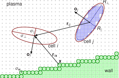
Figure 2: (Color online) Outline of our 3D model by means of a 2D cut. Shown are two cells $i$ and $j$ with their axes of rotational symmetry $\mathbf{o}_{i}$ and $\mathbf{o}_{j}$. The volumes defined by the cell-cell interaction is approximately ellipsoidal with half axes $\sigma_{\parallel}$ and $\sigma_{\perp}$ (red, —). The ellipsoidal volume of the cell-plasma interaction with half axes $R_{\parallel}$ and $R_{\perp}$ is discretized on the underlying lattice. It is shown for only one cell (blue, - -). The cell-wall potential assumes spheres with radius $\sigma_{\text{w}}$ on all surface wall nodes (green, —). Depicted are also the center displacement vectors $\mathbf{r}_{ij}$ and $\mathbf{r}_{i\mathbf{x}}$ between both cells and to an arbitrary surface wall node $\mathbf{x}$.

IV Results

As a convention in this work, primed variables are used to distinguish quantities given in physical units from the corresponding unprimed variable measured in lattice units. The maximum extent of physiological RBCs at their equilibrium shape amounts to about $8\,\mu\text{m}$ and $2.6\,\mu\text{m}$ perpendicular and parallel to the axis of rotational symmetry Evans and Fung (1972). We find that an ellipsoid of revolution with the same numbers as axes has a volume of $87\,\mu\text{m}^{3}$ which fits with the RBC volume measured in Evans and Fung (1972). We therefore choose the size parameters of the cell-cell potential to be

$$\sigma^{\prime}_{\perp}=4\,\mu\text{m}\quad\text{and}\quad\sigma^{\prime}_{\parallel}=4/3\,\mu\text{m}$$ (21)

and achieve that both the magnitude and the maximum extents of the volume defined by the cell-cell interaction match typical values for physiological erythrocytes.

All quantities that are of interest in our simulations can be converted from simulation units to physical units by multiplication with products of integer powers of the conversion factors $\delta x$, $\delta t$, and $\delta m$ for space, time, and mass that thus completely define a scale. We determine the mean deviations of the Stokes drag coefficients of a single spherical particle from the theoretical values in the laminar regime to be in the order of $10^{-2}$ for a radius of $2.5$ lattice units. This is in agreement with equivalent tests done by Ladd Ladd (1994). We therefore restrict ourselves to simulations of particles whose representation on the lattice is at least as large as that of a sphere with radius $2.5$. When using the same aspect ratio $R_{\perp}/R_{\parallel}=\sigma_{\perp}/\sigma_{\parallel}=3$ for the cell-fluid as for the cell-cell interaction, this requirement results in minimum values for $R_{\perp}$ and $R_{\parallel}$ of $3.6$ and $1.2$ lattice units, respectively.

It can be expected that with cell-fluid volumes that are significantly smaller than the size parameters of the potential we cannot achieve realistic coupling strengths which are needed for example to model the clogging of capillaries. Still, $R_{\perp}$ and $R_{\parallel}$ should be smaller than the respective size parameters of the cell-cell potential since limiting the amount of overlapping cell-fluid interaction volume will improve the modeling of hydrodynamics between cells. Ladd et al. Ladd and Verberg (2001) suggest assisting the particle-fluid coupling method with lubrication corrections starting at gap widths below $2/3$ lattice spacings. Throughout this work, we choose $\delta x=2/3\,\mu\text{m}$ as a compromise that both keeps the resolution and the computational cost low and allows one to combine—for example—a high ratio of $R_{\parallel}/\sigma_{\parallel}=7/8$ with a minimum gap width of $2(\sigma_{\parallel}-R_{\parallel})=0.5$ at which the cell-cell potential starts to set in.

To improve the numerical stability of the LB method and to easily relate given input radii $R_{\parallel}$ and $R_{\perp}$ to an effective particle size Ladd (1994), we always set the relaxation time to $\tau=1$. This, together with the constraint

$$\nu\frac{\delta x^{2}}{\delta t}=\frac{2\tau-1}{6}\frac{\delta x^{2}}{\delta t}=1.09\times 10^{-6}\frac{\text{m}^{2}}{\text{s}}=\nu^{\prime}$$ (22)

caused by the fact that the simulated kinematic fluid viscosity $\nu$ is supposed to match the kinematic viscosity of blood plasma of $\nu^{\prime}=1.09\times 10^{-6}\,\text{m}^{2}/\text{s}$ when converted to physical units, determines the time discretization as $\delta t=6.80\times 10^{-8}\,\text{s}$. For convenience, we arbitrarily choose the fluid density in simulation units to be $\bar{\rho}=1$. With $\delta x$ and the physical plasma density $\bar{\rho}^{\prime}=1.03\times 10^{3}\,\text{kg}/\text{m}^{3}$, this choice results in a mass conversion factor of $\delta m=3.05\times 10^{-16}\,\text{kg}$.

We first investigate the effects of the free model parameters by measuring the ratio of the apparent dynamic viscosity $\mu_{\text{app}}$ and the constant plasma viscosity $\mu$ for a homogeneous suspension of cells in plane Couette flow. All simulations reported here are performed on a system with a size of $l_{x}=128$ lattice units in $x$- and at least $l_{y}=l_{z}=40$ lattice units in $y$- and $z$-direction. This represents $85\times 27^{2}\,\mu\text{m}^{3}$ of real blood. Between the two $yz$-side planes a constant offset of the local fluid velocities in $z$-direction is imposed by an adaption of the Lees-Edwards shear boundary condition to the LB method Lees and Edwards (1972); Wagner and Yeomans (1999). The other edges are linked purely periodically. For the cells, we implement a reflective boundary condition that negates the normal velocity component of a cell as soon as its center distance to one of the sheared side planes becomes less than $\sigma_{\perp}$. This procedure surely is inconsistent with respect to the open boundaries implemented for the fluid but far easier to achieve than a common Lees-Edwards implementation for both phases. To prevent these boundaries from influencing our measurements, we determine the shear rate $\dot{\gamma}$ only in the central half of the system where the flow resembles an unbounded Couette flow. We obtain $\dot{\gamma}$ from a linear fit of the velocity profile $v_{z}(x)$. The apparent viscosity

$$\mu_{\text{app}}=\frac{\Delta p_{\text{LE},z}}{l_{y}l_{z}\dot{\gamma}}$$ (23)

is then calculated based on $\Delta p_{\text{LE},z}$ which is the averaged $z$-momentum transfer across both Lees-Edwards boundaries during one time step. For each shear rate, we start with resting and randomly oriented model cells suspended in likewise resting fluid. We calculate Eq. 23 in intervals during the simulation and start accumulating the result for temporal averaging as soon as a steady state is achieved. Several samples prove that neither the change of the random seed for the generation of the initial cell configuration nor the stepwise increase of the system size perpendicular to the velocity gradient up to a volume of $85^{3}\,\mu\text{m}^{3}$ leads to any significant deviation of the results. However, we find that the shear causes the cell orientations $\{\hat{\mathbf{o}}_{i}\}$ to preferably align in the $xz$-plane.

A proper choice of the ratio $R_{\parallel}/\sigma_{\parallel}$ is not known a priori. We thus perform simulations at a constant shear rate of $\dot{\gamma}=(2.21\pm 0.08)\times 10^{3}\,\text{s}^{-1}$ for different $R_{\parallel}/\sigma_{\parallel}$. The resulting particle Reynolds numbers $Re_{\text{P}}$ are of the order of $10^{-1}$. We arbitrarily choose a cell number density of $p^{\prime}=(6.4\pm 0.3)\times 10^{15}\,\mathrm{m}^{-3}$ corresponding to a physiological hematocrit of $56\,\%$ and a cell stiffness parameter of $\bar{\varepsilon}^{\prime}=1.47\times 10^{-15}\,\text{J}$. The resulting apparent viscosity $\mu_{\text{app}}$ as a function of the ratio $R_{\parallel}/\sigma_{\parallel}$ is drawn in Fig. 3. A relatively mild and almost linear increase is visible for $R_{\parallel}/\sigma_{\parallel}<1$ which can be related to the increase of friction in the system. Around $1$, the increase becomes considerably steeper as the minimum gaps of approaching cells vanish. At even larger ratios, the slope decreases again due to large and unphysical amounts of overlap of the cell-fluid coupling volumes that accordingly to Eq. 13 and Eq. 14 reduce the effective friction between cells. Based on our previous considerations and affirmed by Fig. 3, we choose $R_{\parallel}/\sigma_{\parallel}=11/12\approx 0.92$ as a value that is close to unity but still induces an only moderate amount of overlap even at high shear rates of the order of $10^{3}\,\text{s}^{-1}$. This choice results in size parameters of the cell-fluid interaction of

$$R^{\prime}_{\perp}=11/3\,\mu\text{m}\quad\text{and}\quad R^{\prime}_{\parallel}=11/9\,\mu\text{m}\text{ .}$$ (24)

All dimensions in Fig. 2 above were already drawn to scale with respect to the dimensional parameters in Eq. 21 and Eq. 24.

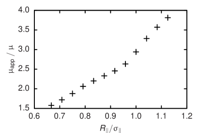
Figure 3: Dependence of the apparent dynamic viscosity $\mu_{\text{app}}$ on the fraction $R_{\parallel}/\sigma_{\parallel}$ of the linear dimensions of the cell-fluid and cell-cell interaction volumes for a shear rate of $\dot{\gamma}^{\prime}=(2.21\pm 0.08)\times 10^{3}\,\text{s}^{-1}$, a number density of $p^{\prime}=(6.4\pm 0.3)\times 10^{15}\,\text{m}^{-3}$, a cell stiffness parameter $\bar{\varepsilon}^{\prime}=1.47\times 10^{-15}\,\text{J}$, and cell-cell size parameters $\sigma_{\perp}^{\prime}=4\,\mu\text{m}$ and $\sigma_{\parallel}^{\prime}=4/3\,\mu\text{m}$. All consecutive simulations are performed with $R_{\parallel}/\sigma_{\parallel}=11/12\approx 0.92$.

The parameter $\bar{\varepsilon}$ is of special interest since it controls the cell stiffness which describes the deformability of the erythrocytes in our model. From experiments it is known that the shear thinning behavior of blood at high shear rates is related to the deformability of the RBC membrane and can be disabled by artificial hardening of the cells Chien (1970); Shin et al. (2004). Our implementation of the model stays numerically stable only for a limited range of $\bar{\varepsilon}$. Simulations performed for various shear rates $1.7\times 10^{1}\,\text{s}^{-1}<\dot{\gamma}<2.3\times 10^{4}\,\text{s}^{-1}$ corresponding to particle Reynolds numbers $10^{-3}\lesssim Re_{\text{P}}\lesssim 1$ and $\bar{\varepsilon}^{\prime}$ varying between $1.47\times 10^{-16}\,\mathrm{J}$ and $1.47\times 10^{-12}\,\mathrm{J}$ at a cell-fluid volume concentration of $43\,\%$ still show that for a given shear rate, larger $\bar{\varepsilon}$ result in higher viscosities yet in a less steep viscosity decrease. Fig. 4 displays this effect which is asymptotically consistent with the experimental results of Chien Chien (1970). It is interesting to note that by plotting the apparent viscosity over the fraction $\dot{\gamma}/\bar{\varepsilon}$—as we do in Fig. 4—we can collapse the region of strongest viscosity decrease in the curves for different $\bar{\varepsilon}$. This indicates that the shear thinning is determined by a balance of viscous and potential forces that scale with $\dot{\gamma}$ and $\bar{\varepsilon}$, respectively. Comparison of Fig. 4 with experimental data taken from the literature Chien (1970) shows best consistency in the case of high shear rates $\dot{\gamma}^{\prime}\sim 10^{3}\,\mathrm{s}^{-1}$ for $\bar{\varepsilon}^{\prime}=1.47\times 10^{-15}\,\mathrm{J}$. We keep this value for all further simulations in the current work.

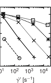
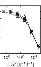
Figure 4: 4 shows the shear rate dependent apparent viscosity $\mu_{\text{app}}$ at a cell-fluid volume concentration of $\Phi_{\text{cf}}=43\,\%$. The different symbols represent different cell stiffness parameters $\bar{\varepsilon}^{\prime}=1.47\times 10^{-k}$ with $k=16,15,14,13,12$ from bottom to top. Rescaling the shear rate $\dot{\gamma}^{\prime}$ with $\bar{\varepsilon}^{\prime}$ as displayed in 4 leads to a collapse of the region of steepest viscosity decrease on a single curve which hints at a concurrence of viscous and potential forces. All further simulations are performed with $k=15$.

Having defined values for all parameters of the cell-fluid and cell-wall interaction, we can now investigate the effect of varying cell concentrations on the viscosity. For given $R_{\parallel}$ and $R_{\perp}$, the cell-fluid volume concentration $\Phi_{\text{cf}}$ is proportional to the number concentration. Fig. 5 shows the dependence of the apparent viscosity on $\Phi_{\text{cf}}$ for a fixed shear rate of $\dot{\gamma}^{\prime}=(2.2\pm 0.1)\times 10^{3}\,\text{s}^{-1}$. The particle Reynolds number is of the order of $Re_{\text{P}}\sim 10^{-1}$. For $\Phi_{\text{cf}}<35\,\%$ we find a nearly linear increase of $\mu_{\text{app}}$. For $\Phi_{\text{cf}}>35\,\%$, the curve is still linear but the slope is slightly smaller. Compared to the literature, $\mu_{\text{app}}$ stays clearly below the viscosities known for hard ellipsoids with a similar aspect ratio of $0.3$ Bertevas et al. (2010). The lower viscosities of our model, especially at high volume fractions, are caused by the reduced dissipation between touching and overlapping cells. This explanation can be substantiated by considering two neighboring boxes of a periodic arrangement each containing one cell in the center. Depending on the orientation and offset relative to the LB grid, direct cell-cell links start to occur at volume concentrations between $30\,\%$ and $50\,\%$ for the given $R_{\perp}$ and $R_{\parallel}$. These numbers also match the region in Fig. 5 where the slope of $\mu_{\text{app}}(\Phi_{\text{cf}})$ decreases. As can be seen from Fig. 5, our results for concentrations up to about $50\,\%$ fit reasonably well with the experimental studies of Goldsmith (see Fung (1981)) and of Shin et al. Shin et al. (2004). At higher $\Phi_{\text{cf}}$, touching cell-fluid volumes start to dominate the rheology of the model suspension. The exact shear rates applied by Goldsmith and Shin et al. are not known. We can only infer from the literature that $\dot{\gamma}^{\prime}$ was larger than $100\,\text{s}^{-1}$ and $250\,\text{s}^{-1}$, respectively. In this range, blood shows shear thinning behavior Chien (1970); Shin et al. (2004) and so does our model (see Fig. 4). It therefore is not possible to determine whether—as Fig. 5 suggests—the model perfectly matches with experiments for $\Phi_{\text{cf}}<40\,\%$ and underestimates the viscosity between $40\,\%$ and $50\,\%$. However, Fig. 4 demonstrates that a better consistency at physiologically important concentrations around $40\,\%$ should be easily attainable by tuning the value of $\bar{\varepsilon}$.

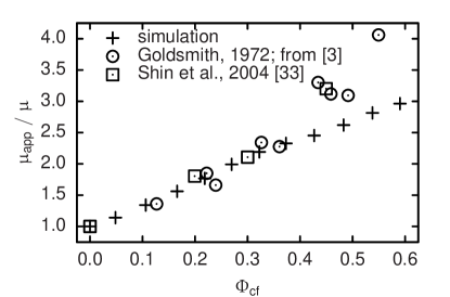
Figure 5: $\mu_{\text{app}}$ dependence on the volume concentration $\Phi_{\text{cf}}$ related to the cell-fluid interaction at a fixed shear rate of $\dot{\gamma}^{\prime}=(2.2\pm 0.1)\times 10^{3}\,\text{s}^{-1}$ compared to experimental data for $\dot{\gamma}^{\prime}>100\,\text{s}^{-1}$ given in Fung (1981); Shin et al. (2004).

While the previous simulations regard bulk properties we now turn to examples where confinement and particulate effects play a crucial role. The cell-wall interaction stiffness $\bar{\varepsilon}_{\text{w}}$ can be determined similarly as $\bar{\varepsilon}$ by comparison with experimental data. As an example we choose the sieving experiments performed by Chien et al. who filtered human erythrocytes through polycarbonate sieves with mean pore diameters of $D^{\prime}=2.2\,\mu\text{m}$ to $4.4\,\mu\text{m}$ and mean pore lengths of $13\,\mu\text{m}$ Chien et al. (1971). They analyzed the resulting flow resistance and damaging of cells in dependence on the pressure drop $\Delta P^{\prime}$ across the sieves which was varied between approximately $10^{2}$ and $10^{5}\,\text{N}/\text{m}^{2}$. We simulate a single cell in front of a pore at a small value of $\Delta P^{\prime}=4\times 10^{2}\,\text{N}/\text{m}^{2}$ ($0.3\,\text{cm}\,\text{Hg}$) and vary the pore diameter and $\bar{\varepsilon}_{\text{w}}$. At this pressure drop, no significant hemolysis, which—as a sub-cell effect—is not resolved in our model, was found in the experiments Chien et al. (1971). However, compared to the case of $D^{\prime}=4.4\,\mu\text{m}$, the flow resistance was increased by a factor of approximately $4$ for $D^{\prime}=3.7\,\mu\text{m}$, by about $30$ for $D^{\prime}=3.0\,\mu\text{m}$, and by more than $100$ for $D^{\prime}=2.2\,\mu\text{m}$ at a hematocrit not higher than of the order of $1\,\%$. In our simulations, we identify the non-passing of model cells with a high increase of flow resistance in the experiments. We find that for $\bar{\varepsilon}^{\prime}_{\text{w}}=1.47\times 10^{-16}\,\text{J}$, the cell passes a pore with only $D^{\prime}=3.0\,\mu\text{m}$ while for $\bar{\varepsilon}^{\prime}_{\text{w}}=1.47\times 10^{-14}\,\text{J}$ already a diameter of $D^{\prime}=4.4\,\mu\text{m}$ proves an insurmountable obstacle. In view of reference Chien et al. (1971) these two $\bar{\varepsilon}_{\text{w}}$ are unrealistic but the intermediate value $\bar{\varepsilon}^{\prime}_{\text{w}}=\bar{\varepsilon}^{\prime}=1.47\times 10^{-15}\,\text{J}$ is an appropriate choice for this setup which allows the model cell to pass through pores with a diameter of $3.7\,\mu\text{m}$ and more. We now study the flow through a bifurcation of cylindrical capillaries with a radius of $4.7\,\mu\text{m}$. One of the branches, however, features a stenosis with radius $R_{\text{s}}$. A cut through the geometry containing nine RBCs is displayed in Fig. 6. It visualizes the cells as the approximated ellipsoidal volumes defined by the zero-energy surface of the cell-cell interaction and the vessel walls as midplane between fluid and wall nodes. The open ends of the system are linked periodically. We drive the system by means of a body force acting only on the fluid in the entrance region. As initial condition, cells are placed randomly in the unconstricted parts of the system. Both, the tube diameters and Reynolds numbers $Re\lesssim 4\times 10^{-3}$ match physiological situations Fung (1981). As above, the cell-wall potential stiffness is chosen to be $\bar{\varepsilon}^{\prime}_{\text{w}}=\bar{\varepsilon}^{\prime}=1.47\times 10^{-15}\,\text{J}$. We average the relative flow rate through the constricted branch $\hat{Q}_{\text{constr}}=Q_{\text{constr}}/(Q_{\text{constr}}+Q_{\text{unconstr}})$ from $1.7\,\text{s}$ to $3.0\,\text{s}$ measured from system initialization. This is done for $R^{\prime}_{\text{s}}=2.7\,\mu\text{m}$, $4.0\,\mu\text{m}$, and $4.7\,\mu\text{m}$. As expected, the results in Fig. 7 are monotonous with $R_{\text{s}}$. When studying the volumetric flow rates of plasma and cells separately, it becomes clear that for $R^{\prime}_{\text{s}}=2.7\,\mu\text{m}$ the cells cannot pass the constriction at the present body force. This situation is visualized in Fig. 6.

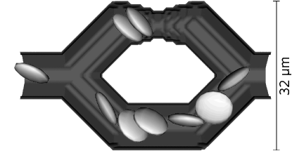
Figure 6: Cut through a capillary bifurcation. Shown are the volumes defined by the cell-cell interaction and the midplane between wall and fluid nodes. The plasma is not visualized. The flow direction is from left to right. The vessel radius is $R^{\prime}_{\text{s}}=2.7\,\mu\text{m}$ at a stenosis in the upper branch and $4.7\,\mu\text{m}$ otherwise. Geometries with length scales that are not large compared to a cell diameter require treatment by a method that is able to resolve particulate effects like the shown clogging of the constricted branch for a cell-wall potential strength of $\bar{\varepsilon}^{\prime}_{\text{w}}=1.47\times 10^{-15}\,\text{J}$.

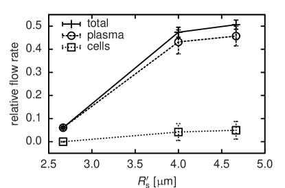
Figure 7: Time-averaged relative flow rate through the constricted capillary in a bifurcation as shown in Fig. 6 for different stenosis radii $R_{\text{s}}$. The cell-wall interaction stiffness is $\bar{\varepsilon}^{\prime}_{\text{w}}=1.47\times 10^{-15}\,\text{J}$. While for $R^{\prime}_{\text{s}}=2.7\,\mu\text{m}$, the constricted branch becomes clogged and only a small amount of plasma passes the remaining aperture, no clogging occurs for larger $R_{\text{s}}$.

We further study the dynamics of the system for the present and two lower cell-wall interaction parameters and plot $\hat{Q}_{\text{constr}}(t)$ in Fig. 8. For $\bar{\varepsilon}^{\prime}_{\text{w}}=1.47\times 10^{-15}\,\text{J}$, the curve decreases in two steps due to the successive arrival of two erythrocytes and stays below $10\,\%$ as only a small amount of plasma is able to pass the remaining aperture. In contrast, there is a continuous flow of plasma and cells for $\bar{\varepsilon}^{\prime}_{\text{w}}=1.47\times 10^{-17}\,\text{J}$. For an intermediate stiffness $\bar{\varepsilon}^{\prime}_{\text{w}}=1.47\times 10^{-16}\,\text{J}$ the cells get stuck initially. However, the flow in the narrowed branch is influenced by the time-dependent cell configuration in the other branch. It happens eventually that the pressure in front of the stenosis rises to a level which lets the RBC overcome the barrier imposed by the cell-wall potential. Each restitution of a higher flow level is initiated by a peak which can be explained by the cell-wall potential that accelerates the RBC into the flow direction while the cell leaves the constriction. As another effect, we find $\bar{\varepsilon}_{\text{w}}$ to affect the relative flow rates of the two phases since larger values force the cells into the center of the capillaries where higher velocities are measured.

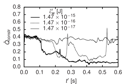
Figure 8: Time evolution of the relative flow rate through the constricted capillary in the bifurcation shown in Fig. 6. For a cell-wall interaction stiffness of $\bar{\varepsilon}^{\prime}_{\text{w}}=1.47\times 10^{-15}\,\text{J}$, the relative flow rate drops to less than $10\,\%$ in two major steps related to the successive arrival of two single erythrocytes at the constriction. With $\bar{\varepsilon}^{\prime}_{\text{w}}=1.47\times 10^{-16}\,\text{J}$, the reduction of the flow rate is only temporary, since the cells are eventually able to pass. While leaving the constriction, the RBCs are accelerated by the cell-wall potential forces which explains the peaks of the flow rate.

Despite the coarse-graining of the model it qualitatively reproduces some aspects of the behavior observed for blood flow in capillaries. The fact that cells approaching a bifurcation show a strong preference to choose the faster branch is described in Fung (1981). The last consequence of this effect is visible in Fig. 6 and Fig. 8 where during a considerable amount of time no further RBCs enter the constricted branch after its closure. It can be seen that our model is able to describe particulate effects which could hardly be covered in terms of a continuous fluid. Obviously, reproducing the behavior of single cells at bifurcations is crucial if the microcirculation and its heterogeneous flow properties are to be modeled Popel and Johnson (2005).

The vessel radii present in the human microvascular system approximately cover a range from $2\,\mu\text{m}$ to $50\,\mu\text{m}$. Having demonstrated the applicability of our model to small capillaries, we proceed with a study of the steady flow through a larger vessel with a radius of $R^{\prime}=31\,\mu\text{m}$ corresponding to an arteriole or venule Popel and Johnson (2005). In the simulation, the vessel is closed periodically at a length of $43\,\mu\text{m}$. We choose $\Phi_{\text{cf}}=42\,\%$ and an intermediate cell-wall interaction stiffness $\bar{\varepsilon}^{\prime}_{\text{w}}=1.47\times 10^{-16}\,\text{J}$. Fig. 9 shows a cut through the vessel for steady flow at $Re\sim 1$. The flow is driven by a body force which acts on both plasma and cells in the whole system and is equivalent to a constant macroscopic pressure gradient. The system is evolved in time until neither the initial fcc ordering of the cells nor significant directed changes in the volumetric flow rate $Q$ are visible. In Fig. 10, the radial velocity profile in the case of a body force resulting in a pseudo-shear rate of $\bar{v}^{\prime}_{z}=Q/(2\pi R^{3})=1.3\times 10^{3}\,\text{s}^{-1}$ or a Reynolds number of $Re\sim 10$ is shown. The graph deviates from the parabolic Hagen-Poiseuille profile that could be observed for a Newtonian fluid. Instead a parabolic core region and a narrow boundary region with high shear rates can be identified. The fit in Fig. 10 shows that this profile can be easily explained by the modified axial-train model as described by Secomb Secomb (2003). The fit parameters are the viscosity ratio of core and boundary $\mu_{\text{c}}/\mu_{\text{b}}$ and the width of the cell-depleted boundary layer $\delta$. The obtained viscosity ratio of $\mu_{\text{c}}/\mu_{\text{b}}=2.43\pm 0.01$ is consistent with the bulk properties in Fig. 5 if we assume $\mu_{\text{b}}=\mu$ and $0.4<\Phi_{\text{cf}}<0.5$ in the core. Also our result of $\delta^{\prime}=(1.47\pm 0.04)\,\mu\text{m}$ seems compatible with the value of $1.8\,\mu\text{m}$ suggested by Secomb Secomb (2003). In additional studies of radial cell-fluid concentration profiles we prove the existence of a cell-depleted layer and the possibility to tune its width by the cell-wall potential stiffness $\bar{\varepsilon}_{\text{w}}$. We also find an increased cell concentration of up to around $\Phi_{\text{cf}}=60\,\%$ close to the central axis of the vessel. This must be a collective effect since in consistency with a 2D study by Qi et al. Qi et al. (2002), we observe that single cells in Poiseuille flow migrate to an intermediate lateral position between vessel wall and center.

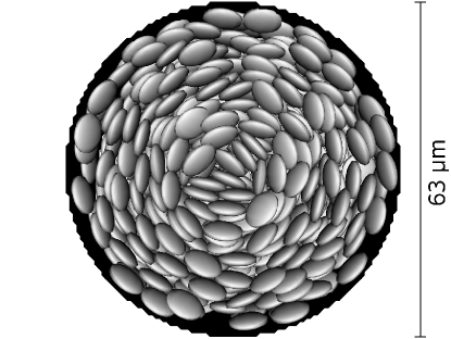
Figure 9: Cut through a cylindrical vessel with a radius of $31\,\mu\text{m}$. For this geometry we choose a cell-wall interaction strength of $\bar{\varepsilon}^{\prime}_{\text{w}}=1.47\times 10^{-16}\,\text{J}$. Shown are the volumes defined by the cell-cell interaction at $42\,\%$ cell-fluid volume concentration and the midplane between wall and fluid nodes. The flow is pointing into the drawing plane and has a maximum velocity of $1.08\times 10^{-2}\,\text{m}/\text{s}$ at the center.

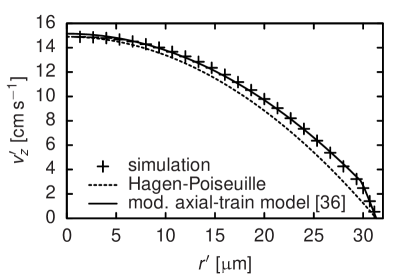
Figure 10: Radial velocity profile in a cylindrical vessel with $42\,\%$ average cell-fluid volume concentration. Apparent slip due to a cell depletion layer is visible. The profile can be well fitted by a modified axial-train model as described by Secomb Secomb (2003). The parabolic Hagen-Poiseuille profile is plotted as well for comparison.

The apparent viscosity for a cylindrical vessel is calculated as

$$\mu_{\text{app}}=\frac{\pi R^{4}}{8Q}\frac{\mathrm{d}P}{\mathrm{d}z}$$ (25)

with $\mathrm{d}P/\mathrm{d}z$ being the macroscopic pressure gradient Popel and Johnson (2005). Pries et al. Pries et al. (1992) present an empirical expression for the dependency of $\mu_{\text{app}}$ on the radius and hematocrit for the case of high flow rates after combining a variety of experimental studies for pseudo-shear rates $\bar{v}^{\prime}_{z}>50\,\text{s}^{-1}$ in a single fit. We perform a series of simulations at $R^{\prime}=31\,\mu\text{m}$ and three fixed pseudo-shear rates between $\bar{v}^{\prime}_{z}=Q/(2\pi R^{3})=(62\pm 1)\,\text{s}^{-1}$ and $(563\pm 3)\,\text{s}^{-1}$ but varying cell-fluid volume concentrations $\Phi_{\text{cf}}$. The corresponding Reynolds numbers are $Re\lesssim 1$. If we identify $\Phi_{\text{cf}}$ with the hematocrit as we do in Fig. 5, we find very good agreement with the relationship by Pries et al. Pries et al. (1992). The comparison is plotted in Fig. 11.

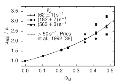
Figure 11: Dependence of the apparent dynamic viscosity $\mu_{\text{app}}$ in a cylindrical vessel with radius $R^{\prime}=31\,\mu\text{m}$ on the cell-fluid volume concentration $\Phi_{\text{cf}}$. Three pseudo-shear rates $\bar{v}^{\prime}_{z}=Q/(2\pi R^{3})$ are examined. The empirical result by Pries et al. Pries et al. (1992) for $\bar{v}^{\prime}_{z}>50\,\text{s}^{-1}$ with $\Phi_{\text{cf}}$ as tube hematocrit is plotted for comparison.

The presence of a cell-depleted layer is closely connected to the emergence of heterogeneous cell concentrations in different parts of the microvasculature since branching daughter-vessels first of all drain blood from the boundary layer Fung (1981). The hematocrit, in turn, influences the flow resistance, the flow rate, and the resulting distribution of erythrocytes at branching points Popel and Johnson (2005). Our simulation approach reproduces these aspects at least qualitatively. When implemented together with an indexed LB scheme as in Axner et al. (2008); Mazzeo and Coveney (2008); Bernaschi et al. (2009), the method will be able to simulate flow through digitized vessel networks covering the whole scale of the microcirculation with high efficiency. Such simulations are still computationally demanding despite the simplifications of the model. Thus even systems that are small in physical units require parallel supercomputers which makes the scalability of the code crucial. For a quasi-homogeneous chunk of suspension consisting of $1024^{2}\times 2048$ lattice sites and $4.1\times 10^{6}$ cells simulated on a BlueGene/P system, we achieve a parallel efficiency normalized to the case of $2048$-fold parallelism of $95.7\,\%$ on $16384$ and still $85.2\,\%$ on $32768$ cores. In comparison, the pure LB code without the MD routines that are responsible for the description of the cells shows a relative parallel efficiency of $98.1\,\%$ on $32768$ cores. The parallel performance of the combined code is mainly limited by the relation of the interaction range of a cell to the size of the computational domain dedicated to each task. We are aware of only one work on simulations of comparably large systems with a particulate description of hemodynamics. This work was published by the group of Aidun and models the deformation of cells explicitly Wu and Aidun (2010); Aidun and Clausen (2010). However, owing to the coarse-graining, our model is easier to parallelize efficiently and—compared to the resolution given in Aidun and Clausen (2010)—allows for substantially higher cell numbers. Generally, our relatively low spatial resolution is highly beneficial for the simulation of large systems since from Eq. 22 it can be derived that the number of lattice site updates necessary for the simulation of a system with a given physical size for a given physical time interval scales with the fifth power of $1/\delta x$. As for plain LB simulations, this number is a good measure for the computational cost also in the case of our suspension model.

V Conclusion

We developed a new approach for the coarse-grained simulation of suspensions of soft particles. This approach is based on a well-established method for rigid particle suspensions Aidun et al. (1998); Ladd and Verberg (2001) which covers the hydrodynamic long-range interactions and phenomenological model potentials to account for the behavior at small particle separations. A parametrization suitable for the quantitative reproduction of hemorheology at moderate to high shear rates Chien (1970); Fung (1981); Shin et al. (2004) was presented. The cell-wall interaction could be linked to experimental data on a single-cell level Chien et al. (1971). Afterwards, we demonstrated that the model shows a complex particulate behavior in bifurcations of partly constricted capillaries which is an essential feature also of the flow properties of the microcirculation in vivo Popel and Johnson (2005). Using the example of steady flow through larger vessels, we proved the existence of a cell-depleted layer and obtained radial velocity profiles that are consistent with an accordant theoretical model Secomb (2003). We could even quantitatively reproduce the experimentally observed dependency of the apparent viscosity in this geometry on the hematocrit Pries et al. (1992). These results suggest that following our approach one can reproduce the particulate behavior of blood on a range of spatial scales that up to this moment was not covered by a single existing simulation method with comparable efficiency. Clearly, our motivation is not to replace models with higher resolution like the ones presented in Sun and Munn (2006); Dupin et al. (2008); McWhirter et al. (2009); Wu and Aidun (2010), but to bridge the gap to continuous descriptions of blood. We believe that this method can prove both an efficient tool for coarse grained yet particulate simulations of flow in microvascular vessel networks and a valuable contribution to the improvement of macroscopic blood modeling.