PACS and SPIRE photometer maps of M33: First results of the Herschel  M33 extended survey (HERM33ES)

Abstract

Context. Within the framework of the HERM33ES key project, we are studying the star forming interstellar medium in the nearby, metal-poor spiral galaxy M33, exploiting the high resolution and sensitivity of Herschel.

Aims. We use PACS and SPIRE maps at 100, 160, 250, 350, and 500 $\mu$m wavelength, to study the variation of the spectral energy distributions (SEDs) with galacto-centric distance.

Methods. Detailed SED modeling is performed using azimuthally averaged fluxes in elliptical rings of 2 kpc width, out to 8 kpc galacto-centric distance. Simple isothermal and two-component grey body models, with fixed dust emissivity index, are fitted to the SEDs between 24 $\mu$m and 500$\,\mu$m using also MIPS/Spitzer  data, to derive first estimates of the dust physical conditions.

Results. The far-infrared and submillimeter maps reveal the branched, knotted spiral structure of M33. An underlying diffuse disk is seen in all SPIRE maps (250–500 $\mu$m). Two component fits to the SEDs agree better than isothermal models with the observed, total and radially averaged flux densities. The two component model, with $\beta$ fixed at 1.5, best fits the global and the radial SEDs. The cold dust component clearly dominates; the relative mass of the warm component is less than 0.3% for all the fits. The temperature of the warm component is not well constrained and is found to be about 60 K$\pm$10 K. The temperature of the cold component drops significantly from $\sim 24$ K in the inner 2 kpc radius to 13 K beyond 6 kpc radial distance, for the best fitting model. The gas-to-dust ratio for $\beta=1.5$, averaged over the galaxy, is higher than the solar value by a factor of 1.5 and is roughly in agreement with the subsolar metallicity of M33.

1 Introduction

In the local universe, most of the observable matter is contained in stellar objects that shape the morphology and dynamics of their “parent” galaxy. In view of the dominance of stellar mass, a better understanding of star formation and its consequences is mandatory. There exists a large number of high spatial resolution studies related to individual star forming regions of the Milky Way, as well as of low linear resolution studies of external galaxies. For a comprehensive view onto the physical and chemical processes driving star formation and galactic evolution it is, however, essential to combine local conditions affecting individual star formation with properties only becoming apparent on global scales.

At a distance of 840 kpc (Freedman et al. 1991), M33 is the only nearby, gas rich disk galaxy that allows a coherent survey at high spatial resolution. It does not suffer from any distance ambiguity, as studies of the Milky Way do, and it is not as inclined as the Andromeda galaxy. M33 is a regular, relatively unperturbed disk galaxy, as opposed to the nearer Magellanic Clouds, which are highly disturbed irregular dwarf galaxies.

M33 is among the best studied galaxies; it has been observed extensively at radio, millimeter, far-infrared (FIR), optical, and X-ray wavelengths, ensuring a readily accessible multi-wavelength database. These data trace the various phases of the interstellar medium (ISM), the hot and diffuse, the warm and atomic, as well as the cold, dense, star forming phases, in addition to the stellar component. However, submillimeter and far-infrared data at high angular and spectral resolutions have been missing so far.

In the framework of the open time key project “Herschel  M33 extended survey (HERM33ES)”, we use all three instruments onboard the ESA Herschel  Space Observatory (Pilbratt et al. 2010) to study the dusty and gaseous ISM in M33. One focus of HERM33ES is on maps of the FIR continuum observed with PACS (Poglitsch et al. 2010) and SPIRE (Griffin et al. 2010), covering the entire galaxy. A second focus lies on observing diagnostic FIR and submillimeter cooling lines [C ii], [O i], [N ii], and H₂O, toward a $2^{\prime}\times 40^{\prime}$ strip along the major axis with PACS and HIFI (de Graauw et al. 2010).

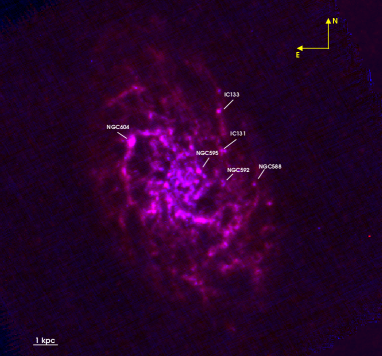
Figure 1: A composite 500 $\mu$m (red) and 160$\,\mu$m (blue) map of M33. The most extended emission is traced by the longest wavelength map revealing the presence of the cold dust in the outskirts of the galaxy. The shorter wavelengths mostly trace the branched spiral structure as well as distinct warm H ii regions and star-forming complexes (such as the ones labeled).

In this first HERM33ES paper, we use continuum maps covering the full extent of M33, at 100, 160, 250, 350, and $500\,\mu$m. These data are an improvement over previous data sets of M33, obtained with ISO and Spitzer  (Hippelein et al. 2003; Hinz et al. 2004; Tabatabaei et al. 2007), in terms of wavelength coverage and angular resolution.

The total bolometric luminosity of normal galaxies is only about a factor of 2 larger than the total IR continuum emission (Hauser & Dwek 2001), which in turn accounts for more than $\sim 98$% of the emission of the ISM (dust$+$gas) (e.g. Malhotra et al. 2001; Dale et al. 2001). Massive star formation heats the dust mainly via its far-ultraviolet (FUV) photons and the absorbed energy is then reradiated in the IR. FIR continuum fluxes are therefore often used as a measure of the interstellar radiation field (ISRF) (e.g. Kramer et al. 2005) and the star formation rate (SFR) (e.g. Schuster et al. 2007). However, a number of authors have suggested that half of the FIR emission or more is due to dust heated by a diffuse ISRF, and not directly linked to massive star formation (Israel et al. 1996; Verley et al. 2009).

Another disputed topic is the evidence for a massive, cold dust component in galaxies. The SCUBA Local Universe Galaxy Survey (Dunne & Eales 2001) identified a cold dust component at an average temperature of 21 K. A number of studies of the millimeter continuum emission of galaxies found indications for even lower temperatures (Misiriotis et al. 2006; Weiß et al. 2008; Liu et al. 2010). In order to estimate the amount of dust at temperatures below about 20 K, and to improve our understanding of the physical conditions of the big grains, well calibrated observations longward of $\sim 150\,\mu$m wavelength are needed.

2 Observations

M33 was mapped with PACS & SPIRE in parallel mode in two orthogonal directions, in 6.3 hours on January 7, 2010. Observations were executed with slow scan speed of $20^{\prime\prime}$/sec, covering a region of about $70^{\prime}\times 70^{\prime}$. Data were taken simultaneously with the PACS green and red channel, centered on 100 and 160$\,\mu$m. SPIRE observations were taken simultaneously at 250, 350, and 500$\,\mu$m. The PACS and the SPIRE data sets were both reduced using the Herschel  Interactive Processing Environment (HIPE) 2.0, with in-house reduction scripts based on the two standard reduction pipelines.

2.1 PACS data

The maps are produced with “photproject”, the default map maker of the PACS data processing pipeline, and a two-step masking technique. First we generate a “naive” map, i.e. not properly taking into account partial pixel overlaps and geometric deformation of the bolometer matrix, and build a mask considering that all pixels above a given threshold do not belong to the sky. Then we use this mask to run the high-pass filter (HPF) taking into account this map. The mask helps to preserve the diffuse component to some extent. With new HIPE tools becoming available, we will try improving data processing to fully recover the diffuse emission in the PACS maps (cf. Fig 1). The final map is built using the filtered, deglitched frames. They have a pixel size of 3.2″ at 100 $\mu$m and 6.4″ at 160 $\mu$m. The spatial resolutions of the PACS data are $6.7^{\prime\prime}\times 6.9^{\prime\prime}$ at 100$\,\mu$m and $10.7^{\prime\prime}\times 12.1^{\prime\prime}$ at 160$\,\mu$m. The pipeline processed data were divided by 1.29 in the red band and 1.09 in the green one, as this correction is not yet implemented in HIPE 2.0. The rms noise levels of the PACS maps are 2.6 mJy pix^-2 at 100 $\mu$m and 6.9 mJy pix^-2 at 160 $\mu$m. The background of the PACS maps of M33 shows perpendicular stripes in each scanning direction due to 1/$f$ noise.

2.2 SPIRE data

A baseline fitting algorithm (Bendo et al. 2010) was applied to every scan of the maps. Next, a “naive” mapping projection was applied to the data and maps with pixel size of $6^{\prime\prime},10^{\prime\prime}$, and $14^{\prime\prime}$ were created for the 250, 350, and 500$\,\mu$m data, respectively. Calibration correction factors of 1.02, 1.05, and 0.94 were applied to the 250, 350, and 500$\,\mu$m maps, as this is not yet implemented in HIPE 2.0. The spatial resolutions are $18.7^{\prime\prime}\times 17.5^{\prime\prime}$, $26.3^{\prime\prime}\times 23.4^{\prime\prime}$, and $38.1^{\prime\prime}\times 35.1^{\prime\prime}$ at 250, 350, and 500$\,\mu$m, respectively. The calibration accuracy is $15\%$. The rms noise levels of the SPIRE maps of M33 are 14.1, 9.2, and 8 mJy/beam, at 250, 350, 500$\,\mu$m.

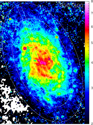
Figure 2: Ratio map of the $250\,\mu$m over $500\,\mu$m maps, at $40^{\prime\prime}$ resolution. Ellipses denote 2, 4, 6, 8 kpc galacto-centric distances with inclination $56^{\circ}$ (Regan & Vogel 1994) and position angle $22.5^{\circ}$ (Paturel et al. 2003). The rectangle delineates the $2^{\prime}\times 40^{\prime}$ wide strip along the major axis, which will be mapped with HIFI and PACS in spectroscopy mode. Crosses mark the H ii regions shown in Fig. 1.

3 Results

3.1 Maps

Figure 1 shows a composite image of the 160$\,\mu$m, 250$\,\mu$m, and 500$\,\mu$m PACS and SPIRE maps. All data sets show the flocculent and knotted spiral arm structure, extending slightly beyond 4 kpc radial distance. The PACS $160\,\mu$m map provides the most detailed view, thanks to its unprecedented linear resolution of 50 pc, allowing to resolve individual giant molecular clouds (GMCs) over the entire disk of M33. A large number of distinct sources delineates the spiral arms. The properties of these sources are studied by Verley et al. (2010) and Boquien et al. (2010). The SPIRE data show a faint, diffuse disk, extending out to $\sim 7$ kpc. Outside of 8 kpc, both maps show some weak emission.

Galactic cirrus is evident only in the outermost part of the galaxy beyond 6 kpc radial distance, showing an average contamination of the order of 2% which can go up to 8% at the very faint levels at 500 $\mu$m. This is still below the 15% calibration error, which is the dominant part of the uncertainty. We did not correct the M33 data for Galactic Cirrus emission.

The $S(250\,\mu{\rm m})/S(500\,\mu{\rm m})$ ratio of flux densities (Fig. 2) drops from about $6$ in the inner spiral arms, to $\sim 4$ at $\sim 4\,$kpc radius, continuing to less than $\sim 3$ at more than 6 kpc radial distance. This drop is also seen in the radially averaged spectral energy distributions (Fig. 3, Table 1). In addition, the inner spiral arms and a couple of prominent H ii regions (cf. Fig. 1), out to about $5$ kpc radius, show an enhanced ratio of $\sim 6$ relative to the inter-arm ISM, exhibiting a ratio of typically $\sim 4$. This shows that dust is mainly heated by the young massive stars rather than the general interstellar radiation field in M33. This is in agreement with a multi-scale study of MIPS data (Tabatabaei et al. 2007), where the 160 $\mu$m emission was found to be well correlated with H$\alpha$ emission. .

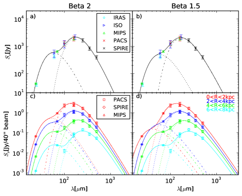
Figure 3: Spectral energy distributions (SEDs) of M33 at wavelengths between 24$\,\mu$m and 500$\,\mu$m. a, b: Total integrated SED of M33, combining data of PACS & SPIRE, with data of MIPS/Spitzer  (Tabatabaei et al. 2007), ISOCAM (Hippelein et al. 2003), and IRAS (Rice et al. 1990). c, d: Radially averaged SEDs in zones of 2 kpc width. Here, we show the MIPS, PACS, and SPIRE data. a, c: Drawn lines show two-component grey body model fit results. The 100 $\mu$m PACS flux density, measured in the outermost zone, was not used for the fits (see the text). The dust emissivity index was set to $\beta=2$. b, d: Drawn lines show two-component models for $\beta=1.5$. a-d: All fits are weighted by the assumed uncertainties: 7% for MIPS 24, 70$\,\mu$m (Spitzer  Observers Manual v8.0), 20% for PACS, 15% for SPIRE. The SEDs have not been de-projected.

Table 1: Results of fits of one and two emission components to the measured spectral energy distributions (SEDs) of the MIPS, PACS, SPIRE data of M33 shown in Figure 3.

	Total	(1)	(2)	(3)	(4)
Isothermal fits
$T$/[K]	29	25	28	105	37
$\beta$	0.5	1.4	0.8	$-1.8$	$-0.8$
$\chi^{2}_{\rm red}$	45	44	45	3	6
Two-component fits with $\beta=2$
$T_{c}$/[K]	16	20	17	14	12
$T_{w}$/[K]	50	55	51	49	48
$M_{c}$/[$10^{6}\,$M⊙]	8.0	1.0	2.4	3.6	4.0
$M_{c}/M_{w}$	1000	900	900	1700	5600
$\chi^{2}_{\rm red}$	0.41	0.23	0.33	0.42	1.8
$M_{\rm gas}/M_{c}$	250	230	180	160	200
Two-component fits with $\beta=1.5$
$T_{c}$/[K]	19	24	20	16	13
$T_{w}$/[K]	55	77	57	52	51
$M_{c}$/[$10^{6}$ M⊙]	10	1.2	3.0	4.6	4.9
$M_{c}/M_{w}$	500	3800	480	730	2200
$\chi^{2}_{\rm red}$	0.14	0.10	0.12	0.20	1.8
$M_{\rm gas}/M_{c}$	200	190	150	120	160
Two-component fits with $\beta=1$
$T_{c}$/[K]	23	28	24	19	15
$T_{w}$/[K]	62	-	67	57	55
$M_{c}$/[$10^{6}\,$M⊙]	12	1.6	3.6	5.7	5.8
$M_{c}/M_{w}$	300	-	440	330	870
$\chi^{2}_{\rm red}$	0.22	0.6	0.26	0.30	2.4
$M_{\rm gas}/M_{c}$	170	140	120	100	140
Total gas mass
$M_{\rm gas}/[10^{6}\,$M⊙]	2020	230	440	560	790

3.2 Spectral energy distributions (SEDs)

Figure 3 shows the total flux densities of M33 and radially averaged SEDs. The SEDs at different annuli were created by smoothing all data to a common resolution of $40^{\prime\prime}$, and averaging the observed flux densities in radial zones of 2 kpc width: $r_{i}\leq R<r_{i}+2\,{\rm kpc}$ with $r_{i}=0,2,4,6$ kpc (cf. Fig. 2). The Herschel  data agree in general well with the data from the literature. The MIPS data at 160$\,\mu$m agree within 20% with the corresponding PACS data, for all radial zones. The 100 $\mu$m PACS flux density, measured in the outermost annulus, is far below the expected value, indicating that extended, diffuse emission is at present lost by the data processing. We do not use these data for the fits.

Figure 3c,d shows the drop of emission by almost two orders of magnitude between the center and the outskirts at 8 kpc radial distance. One striking feature of the radially averaged SEDs is the change of the 160/250 PACS/SPIRE flux density ratio (color), which drops systematically with radial distance, from 1.7 in the inner zone, to 0.5 in the outer zone. At the same time, the slope of the SPIRE data turns shallower with distance, as already seen in Fig. 2.

We fit simple isothermal and two-component grey body models to the data. Each component is described by $S_{\nu}=B(\nu,T)\tau_{\nu}=B(\nu,T)\kappa_{\nu}M_{d}/D^{2}$, assuming optically thin emission, with the flux $S_{\nu}$, the Planck function $B_{\nu}$, the opacity $\tau_{\nu}$, the dust mass $M_{d}$, the distance $D$, and the dust absorption coefficient $\kappa_{\nu}=0.4(\nu/(250\,{\rm GHz}))^{\beta}$ cm²g^-1 (Kruegel & Siebenmorgen 1994; Kruegel 2003), $\beta$ is the dust emissivity index. The fit minimizes the function $\chi^{2}=\sum((S_{\nu,{\rm obs}}-S_{\nu})/\Delta S_{\nu,{\rm obs}})^{2}$ using the Levenberg-Marquardt algorithm (Bevington & Robinson 1992), with the assumed calibration error $\Delta S_{\nu,{\rm obs}}$. The fits are conducted at 7 wavelengths using the SPIRE, PACS, and the MIPS data at 70 and 24 $\mu$m. The 24 $\mu$m data helps in constraining the warm component, though its emission partly stems from stochastically heated small grains, not only from grains in thermal equilibrium. To maintain at least two degrees of freedom (Bevington & Robinson 1992) in the 2-component fit, we kept $\beta$ fixed to values between 1 and 2. These values are typically found in models and observations of interstellar dust (see literature compiled by Dunne & Eales 2001).

The fits of isothermal models do not reproduce the data well, the values of the reduced $\chi^{2}$ are very high. To a large extent, this is because of the 24 $\mu$m points, which clearly require a second, warm dust component. Two-component grey body models result in a much better agreement with the data. The best fitting model is the two-component model with $\beta=1.5$. The $\chi^{2}_{\rm red}$ values are better than 0.2 for all annuli out to 6 kpc, and 1.8 for the outermost annulus. However, these values are only slightly better or equal to the $\chi^{2}_{\rm red}$ values of the two other two-component models.

We find higher temperatures of the cold component for lower values of $\beta$, rendering it difficult to determine both parameters at the same time. This degeneracy between dust temperature and dust emissivity is a common problem (e.g. Kramer et al. 2003). Note, however, that the total mass of the cold component, is rather well determined. For $\beta$-values varying between 1 and 2, this mass only varies by $\sim 20$%. The masses in each annulus were determined by fitting the observed SEDs. As the fitted temperatures are slightly different, the sum over the four annuli does not exactly agree with the fitted total cold dust mass in Table 1.

The cold dust component dominates the mass for the galaxy for all annuli. Though the warm component is needed to reproduce the data shortwards of $\sim 100\,\mu$m, its relative mass is less than 0.3% for all cases. Therefore, its temperature is not well constrained. It is found to be about 60 K$\pm$10 K. The temperature of the cold component is determined to an accuracy of about 3 K, as estimated from a Monte Carlo analysis using the observed data with the estimated accuracies. It drops significantly from $\sim 24$ K in the inner 2 kpc radius to 13 K beyond 6 kpc radial distance, using the best fitting model.

Table 1 also gives the total gas masses $M_{\rm gas}$ of the entire galaxy, and of the elliptical annuli. These are calculated from H i and CO data presented in Gratier et al. (2010). They assume a constant CO-to-H₂ conversion factor. But note that this X_CO factor does not strongly affect the total gas masses, as the H i is dominating. The gas-to-dust mass ratio for the entire galaxy, using the best fitting dust model with $\beta=1.5$, is $\sim 200$, about a factor of 1.5 higher than the solar value of 137 (cf. Table 2 in Draine et al. 2007), and a factor of 2 higher than recent dust models for the Milky Way (Weingartner & Draine 2001; Draine et al. 2007). A factor of about 2 is expected, as the metallicity is about half solar (Magrini et al. 2009). The gas-to-dust ratio for $\beta=1.5$ varies between 200 and 120 in the different annuli. Within our errors this is consistent with the shallow O/H abundance gradient found by Magrini et al. (2009). The gas-to-dust ratios found in M33 are similar to the typical values found in nearby galaxies (e.g. Draine et al. 2007; Bendo et al. 2010). Braine et al. (2010) combine the dust and gas data of M33 to study the gas-to-dust ratios in more detail and derive dust cross sections.