Decoupling the NLO coupled DGLAP evolution equations: an analytic solution to pQCD

Abstract

Using repeated Laplace transform techniques, along with newly-developed accurate numerical inverse Laplace transform algorithms Block (2010a, b), we transform the coupled, integral-differential NLO singlet DGLAP equations first into coupled differential equations, then into coupled algebraic equations, which we can solve iteratively. After Laplace inverting the algebraic solution analytically, we numerically invert the solutions of the decoupled differential equations. Finally, we arrive at the decoupled NLO evolved solutions

$$F_{s}(x,Q^{2}) = {\cal F}_{s}(F_{s0}(x),G_{0}(x)),$$

$$G(x,Q^{2}) = {\cal G}(F_{s0}(x),G_{0}(x)),$$

where ${\cal F}_{s}$ and $\cal G$ are known functions- determined using the DGLAP splitting functions up to NLO in the strong coupling constant $\alpha_{s}(Q^{2})$. The functions $F_{s0}(x)\equiv F_{s}(x,Q_{0}^{2})$ and $G_{0}(x)\equiv G(x,Q_{0}^{2})$ are the starting functions for the evolution at $Q^{2}=Q_{0}^{2}$. This approach furnishes us with a new tool for readily obtaining, independently, the effects of the starting functions on either the evolved gluon or singlet structure functions, as a function of both $Q^{2}$ and $Q_{0}^{2}$. It is not necessary to evolve coupled integral-differential equations numerically on a two-dimensional grid, as is currently done. The same approach can be used for NLO non-singlet distributions where it is simpler, only requiring one Laplace transform. We make successful NLO numerical comparisons to two non-singlet distributions, using NLO quark distributions published by the MSTW collaboration Martin et al. (2009), over a large range of $x$ and $Q^{2}$. Our method is readily generalized to higher orders in the strong coupling constant $\alpha_{s}(Q^{2})$.

I Introduction

In order to interpret the experimental results at the Large Hadron Collider—in the search for new physics—accurate knowledge of gluon distribution functions at small Bjorken $x$ and large virtuality $Q^{2}$ plays a vital role in estimating QCD backgrounds and in calculating gluon-initiated processes. The gluon and quark distribution functions have traditionally been determined simultaneously by fitting experimental data on neutral- and charged-current deep inelastic scattering processes and some jet data over a large domain of values of $x$ and $Q^{2}$. The distributions at small $x$ and large $Q^{2}$ are determined mainly by the proton structure function $F_{2}^{\gamma p}(x,Q^{2})$ measured in deep inelastic $ep$ (or $\gamma^{*}p$) scattering. The fitting process starts with an initial $Q^{2}_{0}$, typically less than $m_{c}^{2}$, the square of the $c$ quark mass of $\approx 2$ GeV², and individual quark and gluon initial distributions which are parameterized with pre-determined shapes in $x$ determined by a set of adjustable input parameters—given as functions of $x$ for the chosen $Q_{0}^{2}$. The distributions are then evolved numerically on a two-dimensional grid in $x$ and $Q^{2}$ to larger $Q^{2}$ using the coupled integral-differential DGLAP equations Gribov and Lipatov (1972); Altarelli and Parisi (1977); Dokshitzer (1977), typically in leading order (LO) and next-to- leading order (NLO), and the results used to predict the measured quantities. The final distributions are then determined by adjusting the input parameters to obtain a best fit to the data. This procedure is very indirect in the case of the gluon: the gluon distribution $G(x,Q^{2})=xg(x,Q^{2})$ does not contribute directly to the accurately determined structure function $F_{2}^{\gamma p}(x,Q^{2})$, and is determined only through the quark distributions in conjunction with the evolution equations, or at large $x$, from jet data. For recent determinations of the gluon and quark distributions, see Pumplin et al. (2002); Tung et al. (2007); Martin et al. (2002, 2004, 2009).

In the following, we will summarize our analytic method that determines the singlet structure function $F_{s}(x,Q^{2})$ and $G(x,Q^{2})$ directly and individually, using as input $F_{s0}(x)\equiv F_{s}(x,Q^{2}_{0})$ and $G_{0}(x)\equiv G(x,Q^{2}_{0})$, where $Q_{0}^{2}$ is arbitrary, with the guarantee that each distribution individually satisfies the NLO coupled DGLAP equations.

The method is extended to calculate NLO non-singlet functions, so that we can also find individual quark and gluon distributions analytically in terms of the starting distributions of the individual quark and gluon distributions. We will also give some numerical examples for non-singlet NLO valence quark distributions, comparing them to the MSTW Martin et al. (2009) published NLO valence quark distributions.

II NLO Singlet Sector

Our approach uses an unusual application of multiple Laplace transforms Block et al. (2008, 2009). In this note, we use double Laplace transforms, first transforming the coupled DGLAP integral-differential equations into a set of coupled differential equations in Laplace space, and finally, into a set of coupled algebraic equations in a second Laplace space. We then solve the coupled algebraic equations in this second Laplace space. To obtain our final results, we must invert the Laplace transforms. The second transform to the algebraic equation space is analytically invertible to the space in which we had the coupled differential equations. The final inversion, from this Laplace space back to our initial space, must be obtained by numerical inverse Laplace transformations Block (2010a, b).

We first introduce the variable $v\equiv\ln(1/x)$ into the NLO coupled DGLAP equations. This turns them into coupled convolution equations in $v$ space, which, after introducing a new variable $\tau(Q^{2},Q^{2}_{0})={1\over 4\pi}\int_{Q_{0}^{2}}^{Q^{2}}\alpha_{s}(Q^{2})d\,\ln Q^{2}$, are readily Laplace transformed to obtain a set of coupled homogeneous first-order differential  equations in the variable $\tau$. The parameters of these transformed equations are known functions of $s$, the Laplace-space variable. These equations are then Laplace transformed a second time, essentially transforming the variable $\tau$ of the coupled differential equations into a new Laplace variable $U$, with the resulting equations being coupled algebraic equations in $U$—with $s$ again being a parameter—which are then solved iteratively. These solutions, in $s$ and $U$, are analytically Laplace inverted back to variables $s$ and $\tau$. Using fast and accurate numerical inverse Laplace transform algorithms Block (2010a, b), we transform the solutions back into $v$ space, and, finally, into Bjorken $x$-space to obtain $F_{s}(x,Q^{2})={\cal F}_{s}(F_{s0}(x),G_{0}(x))$ and $G(x,Q^{2})={\cal G}(F_{s0}(x),G_{0}(x))$, where the functions $\cal F$ and $\cal G$ are determined by the splitting functions in the DGLAP equations.

A similar method was used in an earlier paper Block et al. (2010) in which we obtained the decoupled solutions in LO for both the singlet and the non-singlet sector, using only one Laplace transform. The $\tau$ dependence in that case was trivial, and the decoupled equations could be solved directly. The extra Laplace transform that appears in the present work is necessitated by the nontrivial dependence of the NLO terms on $\tau$.

Our method is readily generalized to all orders in the strong coupling constant, but for brevity we limit ourselves to NLO in this paper. We write the coupled NLO DGLAP equations Block et al. (2008, 2009) schematically, using the convolution symbol $\otimes$, as

$$\frac{4\pi}{\alpha_{s}(Q^{2})}\frac{\partial F_{s}}{\partial\ln{Q^{2}}}(x,Q^{2}) = F_{s}\otimes\left(P_{qq}^{0}+\frac{\alpha_{s}(Q^{2})}{4\pi}P_{qq}^{1}\right)(x,Q^{2})+G\otimes\left(P_{qg}^{0}+\frac{\alpha_{s}(Q^{2})}{4\pi}P_{qg}^{1}\right)(x,Q^{2}),$$ (1)

$$\frac{4\pi}{\alpha_{s}(Q^{2})}\frac{\partial G}{\partial\ln{Q^{2}}}(x,Q^{2}) = F_{s}\otimes\left(P_{gq}^{0}+\frac{\alpha_{s}(Q^{2})}{4\pi}P_{gq}^{1}\right)(x,Q^{2})+G\otimes\left(P_{gg}^{0}+\frac{\alpha_{s}(Q^{2})}{4\pi}P_{qg}^{1}\right)(x,Q^{2}).$$ (2)

The $P_{qq}^{0}(x),\ P_{qg}^{0}(x),\ P_{gq}^{0}(x)$ and $P_{gg}^{0}(x)$ used in Eq. (1) and Eq. (2) are the LO singlet splitting function and the $P_{qq}^{1}(x),\ P_{qg}^{1}(x),\ P_{gq}^{1}(x)$ and $P_{gg}^{1}(x)$ are the NLO singlet splitting functions, with $\alpha_{s}(Q^{2})$ the NLO running strong coupling constant. It is standard procedure to construct $\alpha_{s}(Q^{2})$ assuming three massless quarks, $u,\ d$ and $s$, below the $c$-quark threshold, adjusting the QCD parameter $\Lambda$ at each successive threshold in $Q^{2}$, i,e, at $Q^{2}=M_{c}^{2}$ and $M_{b}^{2}$, so that $\alpha_{s}(Q^{2})$ remains continuous when the number of quarks changes as heavy $c$ and $b$ quarks begin to contribute.

Introducing the variable changes

$$v \equiv \ln(1/x),\quad w\equiv\ln(1/z),\qquad\tau(Q^{2},Q_{0}^{2})\equiv{1\over 4\pi}\int_{Q^{2}_{0}}^{Q^{2}}\alpha_{s}(Q^{\prime 2})d\,\ln Q^{\prime 2},\quad$$ (3)

and the notation

$$\hat{F}_{s}(v,\tau) \equiv F_{s}(e^{-v},Q^{2}),\qquad\hat{G}(v,\tau)\equiv G(e^{-v},Q^{2}),$$ (4)

we rewrite the above DGLAP equations in terms of the convolution integrals

$$\frac{\partial{\hat{F}}_{s}}{\partial\tau}(v,\tau) = \int_{0}^{v}{\hat{F}}_{s}(w,\tau)\left({\hat{H}}_{qq}(v-w)+\frac{\alpha_{s}(\tau)}{4\pi}{\hat{H}}_{qq}^{1}(v-w)\right)d\,w$$ (5)

$$+\int_{0}^{v}{\hat{G}}(w,\tau)\left({\hat{H}}_{qg}(v-w)+\frac{\alpha_{s}(\tau)}{4\pi}{\hat{H}}_{qg}^{1}(v-w)\right)d\,w,$$

$$\frac{\partial{\hat{G}}}{\partial\tau}(v,\tau) = \int_{0}^{v}{\hat{F}}_{s}(w,\tau)\left({\hat{H}}_{gq}(v-w)+\frac{\alpha_{s}(\tau)}{4\pi}{\hat{H}}_{gq}^{1}(v-w)\right)d\,w$$ (6)

$$+\int_{0}^{v}{\hat{G}}(w,\tau)\left({\hat{H}}_{gg}(v-w)+\frac{\alpha_{s}(\tau)}{4\pi}{\hat{H}}_{gg}^{1}(v-w)\right)d\,w,$$

where

$${\hat{F}}_{s}(v,\tau) \equiv F_{s}(e^{-v},\tau),\qquad\hat{G}(v,\tau)\equiv G(e^{-v},\tau),$$ (7)

$${\hat{H}}_{qq}^{0}(v) \equiv e^{-v}P_{qq}^{0}(e^{-v}),\quad{\hat{H}}_{qg}^{0}(v)\equiv e^{-v}P_{qg}^{0}(e^{-v}),\quad{\hat{H}}_{gq}^{0}(v)\equiv e^{-v}P_{gq}^{0}(e^{-v}),\quad{\hat{H}}_{gg}^{0}(v)\equiv e^{-v}P_{gg}^{0}(e^{-v}),$$ (8)

$${\hat{H}}_{qq}^{1}(v) \equiv e^{-v}P_{qq}^{1}(e^{-v}),\quad{\hat{H}}_{qg}^{1}(v)\equiv e^{-v}P_{qg}^{1}(e^{-v}),\quad{\hat{H}}_{gq}^{1}(v)\equiv e^{-v}P_{gq}^{1}(e^{-v}),\quad{\hat{H}}_{gg}^{1}(v)\equiv e^{-v}P_{gg}^{1}(e^{-v}).$$ (9)

The splitting functions $P_{qq}(e^{-v})$ and $P_{gg}(e^{-v})$ in the integrals Eq. (5) and Eq. (6) involve the distribution $1/(1-e^{-v})_{+}$. The integrals involving this term can be transformed to expressions that involve derivatives of ${\hat{F}}_{s}$ or ${\hat{G}}$ without the appearance of the singular factor $1/(1-e^{-v})$, for example, to integrals of the form $\int_{0}^{v}\partial{\hat{F}}_{s}(w,\tau)/\partial{w}\ln[1-e^{-(v-w)}]dw$ and $\int_{0}^{v}\partial{\hat{G}}(w,\tau)/\partial{w}\ln[1-e^{-(v-w)}]dw$. After this change, all of the integrals in Eqs. (5) and (6) are normal convolutions. By making a Laplace transform in $v$, we can factor these integrals, since the Laplace transform of a convolution is the product of the Laplace transform of the factors, i.e.,

$${\cal L}\left[\int_{0}^{v}{\hat{F}}[w]{\hat{H}}[v-w]\,dw;s\right] = {\cal L}[{\hat{F}}[v];s]\times{\cal L}[{\hat{H}}[v];s].$$ (10)

Defining the Laplace transforms

$$f(s,\tau) \equiv {\cal L}\left[\hat{F}_{s}(v,\tau);s\right],\qquad g(s,\tau)\equiv{\cal L}[\hat{G}(v,\tau);s]$$ (11)

and noting that

$${\cal L}\left[{\partial\hat{F}_{s}\over\partial w}(w,\tau);s\right]=sf(s,\tau),\qquad{\cal L}\left[{\partial\hat{G}\over\partial w}(w,\tau);s\right]=sg(s,\tau),$$ (12)

we can factor the Laplace transforms of Eq. (5) and Eq. (6) into two coupled ordinary first order differential equations in the variable $\tau$ in Laplace space $s$ with $\tau$-dependent coefficients. These can be written as

$${\partial f\over\partial\tau}(s,\tau) = \left(\Phi_{f}^{LO}(s)+\frac{\alpha_{s}(\tau)}{4\pi}\Phi_{f}^{NLO}(s)\right)f(s,\tau)+\left(\Theta_{f}^{LO}(s)+\frac{\alpha_{s}(\tau)}{4\pi}\Theta_{f}^{NLO}(s)\right)g(s,\tau),$$ (13)

$${\partial g\over\partial\tau}(s,\tau) = \left(\Phi_{g}^{LO}(s)+\frac{\alpha_{s}(\tau)}{4\pi}\Phi_{g}^{NLO}(s)\right)g(s,\tau)+\left(\Theta_{g}^{LO}(s)+\frac{\alpha_{s}(\tau)}{4\pi}\Theta_{g}^{NLO}(s)\right)f(s,\tau),$$ (14)

where we recall that the the $Q^{2}$ dependence is through the function $\tau$, i.e., $\tau(Q^{2},Q_{0}^{2})={1\over 4\pi}\int_{Q_{0}^{2}}^{Q^{2}}\alpha_{s}(Q^{\prime 2})\,d\,\ln Q^{\prime 2}.$

The LO coefficients $\Phi^{LO}$ and $\Theta^{LO}$ are given by Block et al. (2010)

$$\Phi^{LO}_{f}(s) = 4-{8\over 3}\left({1\over s+1}+{1\over s+2}+2\left(\psi(s+1)+\gamma_{E}\right)\right),$$ (15)

$$\Theta_{f}^{LO}(s) = 2n_{f}\left({1\over s+1}-{2\over s+2}+{2\over s+3}\right),$$ (16)

$$\Phi_{g}^{LO}(s) = {33-2n_{f}\over 3}+12\left({1\over s}-{2\over s+1}+{1\over s+2}-{1\over s+3}-\psi(s+1)-\gamma_{E}\right),$$ (17)

$$\Theta_{g}^{LO}(s) = {8\over 3}\left({2\over s}-{2\over s+1}+{1\over s+2}.\right),$$ (18)

Here $\psi(x)$ in Eqs. (15) and (17) is the digamma function and $\gamma_{E}=0.5772156\ldots$ is Euler’s constant, quantities that are introduced in the Laplace transform of the LO terms involving the distribution $1/(1-e^{-v})_{+}$ discussed above. The evaluation of the NLO coefficients is straightforward, but too lengthy to be included in this note, and will be given, in the future, when we make numerical evaluations of $F_{s}(x,Q^{2})$ and $G(x,Q^{2})$ in NLO.

In the case of LO, the $\tau$ dependence of the equations is trivial, and the equations can be solved simply Block et al. (2010), as already noted. The extra explicit dependence of the NLO terms on the right-hands of these equations on $\tau$ prevents a similar construction here. In order to decouple and solve Eq. (13) and Eq. (14), we Laplace transform them a second time—this time with respect to the variable $\tau$—into $U$ space, i.e., we let

$${\cal F}(s,U) \equiv {\cal L}\left[f(s,\tau);U\right],\qquad{\cal G}(s,U)\equiv{\cal L}\left[g(s,\tau);U\right],$$ (19)

$${\cal L}\left[{\partial f\over\partial\tau}(s,\tau);U\right] = U{\cal F}(s,U)-f_{0}(s),\qquad{\cal L}\left[{\partial g\over\partial\tau}(s,\tau);U\right]=U{\cal G}(s,U)-g_{0}(s),$$ (20)

where now $s$ is simply a parameter in $U$ space.

In $U$ space, we now write the final desired coupled algebraic equations for ${\cal F}(s,U)$ and ${\cal G}(s,U)$ as

$$U{\cal F}(s,U)-f_{0}(s) = \Phi_{f}^{LO}(s){\cal F}(s,U)+\Phi_{f}^{NLO}(s){\cal L}[\frac{\alpha_{s}(\tau)}{4\pi}f(s,\tau);U]$$ (21)

$$+\Theta_{f}^{LO}(s){\cal G}(s,U)+\Theta_{f}^{NLO}(s){\cal L}[\frac{\alpha_{s}(\tau)}{4\pi}g(s,\tau);U],$$

$$U{\cal G}(s,U)-g_{0}(s) = \Phi_{g}^{LO}(s){\cal G}(s,U)+\Phi_{g}^{NLO}(s){\cal L}[\frac{\alpha_{s}(\tau)}{4\pi}g(s,\tau);U]$$ (22)

$$+\Theta_{g}^{LO}(s){\cal F}(s,U)+\Theta_{g}^{NLO}(s){\cal L}[\frac{\alpha_{s}(\tau)}{4\pi}f(s,\tau);U].$$

For brevity, we replace the NLO ${\alpha_{s}(\tau)\over 4\pi}$ by $a(\tau)$ in Eq. (21) and Eq. (22). We can numerically show that an excellent approximation to $a(\tau)\equiv{\alpha_{s}(\tau)\over 4\pi}$, accurate to a few parts in $10^{4}$, is given by the expression

$$a(\tau) \approx a_{0}+a_{1}e^{-b_{1}\tau},$$ (23)

where the constants $a_{0},a_{1},b_{1}$ are found by a least squares fit to $a(\tau)$. We note in passing that this approximation is inspired by the fact that in LO, $\alpha_{s,LO}(\tau)$ is exactly given by the form $\alpha_{s,LO}(Q_{0}^{2})e^{-b\tau}$.

Using the value of $a(\tau)$ given by Eq. (23), we can write the Laplace transforms ${\cal L}[\frac{\alpha_{s}(\tau)}{4\pi}f(s,\tau);U]$ and ${\cal L}[\frac{\alpha_{s}(\tau)}{4\pi}g(s,\tau);U]$ needed in Eq. (21) and Eq. (22) as

$${\cal L}[\frac{\alpha_{s}(\tau)}{4\pi}f(s,\tau);U] = \sum_{j=0}^{1}a_{j}{\cal F}(s,U+b_{j}),\qquad{\cal L}[\frac{\alpha_{s}(\tau)}{4\pi}g(s,\tau);U]=\sum_{j=0}^{1}a_{j}{\cal G}(s,U+b_{j}),$$ (24)

where $b_{0}=0$ is understood in Eq. (23) and Eq. (24).

After introducing the simplifying notation

$$\Phi_{f}(s)\equiv\Phi_{f}^{LO}(s)+a_{0}\Phi_{f}^{NLO}(s),\qquad\Phi_{g}(s)\equiv\Phi_{g}^{LO}(s)+a_{0}\Phi_{g}^{NLO}(s),$$ (25)

$$\Theta_{f}(s)\equiv\Theta_{f}^{LO}(s)+a_{0}\Theta_{f}^{NLO}(s),\qquad\Theta_{g}(s)\equiv\Theta_{g}^{LO}(s)+a_{0}\Theta_{g}^{NLO}(s),$$ (26)

we can finally rewrite Eq. (21) and Eq. (22) as

$$\left[U-\Phi_{f}(s)\right]{\cal F}(s,U)-\Theta_{f}(s){\cal G}(s,U) = f_{0}(s)+a_{1}\left[\Phi_{f}^{NLO}(s){\cal F}(s,U+b_{1})+\Theta_{f}^{NLO}(s){\cal G}(s,U+b_{1})\right],$$ (27)

$$-\Theta_{g}(s){\cal F}(s,U)+\left[U-\Phi_{g}(s)\right]{\cal G}(s,U) = g_{0}(s)+a_{1}\left[\Theta_{g}^{NLO}(s){\cal F}(s,U+b_{1})+\Phi_{g}^{NLO}(s){\cal G}(s,U+b_{1})\right],$$ (28)

which we will solve iteratively, using $a_{1}$ as an expansion parameter.

We note that the $\Phi$’s and $\Theta$’s, as defined above, contain both LO and NLO terms. We further point out that Eq. (27) and Eq. (28) are completely symmetric under the simultaneous transformations $f\leftrightarrow g$ and $\cal F\leftrightarrow\cal G$. We finally remark that $a_{1}$, the NLO expansion parameter in our iterative solution of Eqs. (25) and (26), is quite small: $a_{1}=0.025,\ b_{1}=10.7$ for $M_{c}^{2}<Q^{2}\leq M_{b}^{2}$ GeV² and $a_{1}=0.017,\ b_{1}=8.63$ for $M_{b}^{2}<Q^{2}\leq 10^{5}$ GeV², with the $a_{0}$ terms in Eq. (25) and Eq. (26) being positive and about an order of magnitude smaller than the $a_{1}$ terms.

We next consider the simple solutions to Eq. (27) and Eq. (28), called ${\cal F}_{1}(s,U)$ and ${\cal G}_{1}(s,U)$, that result from setting $a_{1}=0$, i.e., the equations

$$\left[U-\Phi_{f}(s)\right]{\cal F}_{1}(s,U)-\Theta_{f}(s){\cal G}_{1}(U) = f_{0}(s),$$ (29)

$$-\Theta_{g}(s){\cal F}_{1}(U)+\left[U-\Phi_{g}(s)\right]{\cal G}_{1}(s,U) = g_{0}(s),$$ (30)

whose solutions are

$${\cal F}_{1}(s,U) = \left[U-\Phi_{g}(s)\right]f_{0}(s)/D(U,s)+\Theta_{f}(s)g_{0}(s)/D(U,s),$$ (31)

$${\cal G}_{1}(s,U) = \left[U-\Phi_{f}(s)\right]g_{0}(s)/D(U,s)+\Theta_{g}(s)f_{0}(s)/D(U,s).$$ (32)

The denominator $D(U,s)$ in Eqs. (31) and (32) is just the determinant of the coefficients of ${\cal F}(s,U)$ and ${\cal G}(s,U)$ in Eqs. (27) and (28),

$$D(U,s) = \Phi_{f}(s)\Phi_{g}(s)-\Theta_{f}(s)\Theta_{g}(s)-\left[\Phi_{f}(s)+\Phi_{g}(s)\right]U+U^{2}$$ (33)

$$= \left(U-\frac{1}{2}\left(\Phi_{f}(s)+\Phi_{g}(s)\right)-\frac{1}{2}R(s)\right)\left(U-\frac{1}{2}\left(\Phi_{f}(s)+\Phi_{g}(s)\right)+\frac{1}{2}R(s)\right),$$

where $R(s)\equiv\sqrt{\left(\Phi_{f}(s)-\Phi_{g}(s)\right)^{2}+4\Theta_{f}(s)\Theta_{g}(s)}$. The zeros of $D(U,s)$ lead to simple poles in ${\cal F}_{1}$ and ${\cal G}_{1}$ in the $U$ plane. These functions have no other singularities, and decrease as $1/|U|$ for $|U|\rightarrow\infty$. The inverse Laplace transforms of ${\cal F}_{1}(s,U)$ and ${\cal G}_{1}(s,U)$, denoted by $f_{1}(s,\tau)$ and $g_{1}(s,\tau)$, are therefore well defined and simple to calculate. We will write them as

$$f_{1}(s,\tau) = k_{ff_{1}}(s,\tau)f_{0}(s)+k_{fg_{1}}(s,\tau)g_{0}(s),\qquad g_{1}(s,\tau)=k_{gg_{1}}(s,\tau)g_{0}(s)+k_{gf_{1}}(s,\tau)f_{0}(s),$$ (34)

where the coefficient functions in the solution are

$$k_{ff_{1}}(s,\tau) \equiv e^{\frac{{\tau}}{2}\left(\Phi_{f}(s)+\Phi_{g}(s)\right)}\left[\cosh\left({\tau\over 2}R(s)\right)+\frac{\sinh\left({\tau\over 2}R(s)\right)}{R(s)}\left(\Phi_{f}(s)-\Phi_{g}(s)\right)\right],$$ (35)

$$k_{fg_{1}}(s,\tau) \equiv e^{{\tau\over 2}\left(\Phi_{f}(s)+\Phi_{g}(s)\right)}{2\sinh\left({\tau\over 2}R(s)\right)\over R(s)}\,\Theta_{f}(s),$$ (36)

$$k_{gg_{1}}(s,\tau) \equiv e^{{\tau\over 2}\left(\Phi_{f}(s)+\Phi_{g}(s)\right)}\left[\cosh\left({\tau\over 2}R(s)\right)-\frac{\sinh\left({\tau\over 2}R(s)\right)}{R(s)}\left(\Phi_{f}(s)-\Phi_{g}(s)\right)\right],$$ (37)

$$k_{gf_{1}}(s,\tau) \equiv e^{{\tau\over 2}\left(\Phi_{f}(s)+\Phi_{g}(s)\right)}{2\sinh\left({\tau\over 2}R(s)\right)\over R(s)}\,\Theta_{g}(s).$$ (38)

We comment that this solution has small NLO terms in it, arising from the $a_{0}$ term in Eq. (25) and Eq. (26). However, it is identical in form to the LO solution we gave in Ref. Block et al. (2010), and reduces to it if we set $a_{0}=0$.

We next construct an iterative solution to Eqs. (27) and (28) for ${\cal F}$ and ${\cal G}$. We start by substituting the known functions ${\cal F}_{1}$ and ${\cal G}_{1}$ for ${\cal F}$ and ${\cal G}$ on the right hand sides of the equations, and then re-solve the equations to obtain the next approximations ${\cal F}_{2}$ and ${\cal G}_{2}$ for ${\cal F}$ and ${\cal G}$, and then repeat the process. For the first step, we make the replacements

$${\cal F}(s,U+b_{1})\rightarrow{\cal F}_{1}(s,U+b_{1}),\qquad{\cal G}(s,U+b_{1})\rightarrow{\cal G}_{1}(s,U+b_{1}),\qquad$$ (39)

on the right-hand sides of Eqs. (27) and (28) to obtain our first iterative equations for ${\cal F}_{2}(s,U)$ and ${\cal G}_{2}(s,U)$,

$$\left[U-\Phi_{f}(s)\right]{\cal F}_{2}(s,U)-\Theta_{f}(s){\cal G}_{2}(s,U) = f_{0}(s)+a_{1}\left[\Phi_{f}^{NLO}(s){\cal F}_{1}(s,U+b_{1})+\Theta_{f}^{NLO}(s){\cal G}_{1}(s,U+b_{1})\right],$$ (40)

$$-\Theta_{g}(s){\cal F}_{2}(s,U)+\left[U-\Phi_{g}(s)\right]{\cal G}_{2}(s,U) = g_{0}(s)+a_{1}\left[\Theta_{g}^{NLO}(s){\cal F}_{1}(s,U+b_{1})+\Phi_{g}^{NLO}(s){\cal G}_{1}(s,U+b_{1})\right].$$ (41)

The functions ${\cal F}_{1}(s,U)$ and ${\cal G}_{1}(s,U)$ are given analytically by Eq. (31) and Eq. (32), respectively, so that we know them at the argument $(s,U+b_{1})$, needed in the right hand sides of our iterative equations.

Since the functions on the right-hand sides of Eqs. (40) and (41) are known, and the left-hand sides have the same structure as Eqs. (29) and (30), their solutions can be obtained by the substitutions

$$f_{0}(s) \rightarrow f_{0}(s)+a_{1}\left[\Phi_{f}^{NLO}(s){\cal F}_{1}(s,U+b_{1})+\Theta_{f}^{NLO}(s){\cal G}_{1}(s,U+b_{1})\right],$$ (42)

$$g_{0}(s) \rightarrow g_{0}(s)+a_{1}\left[\Theta_{g}^{NLO}(s){\cal F}_{1}(s,U+b_{1})+\Phi_{g}^{NLO}(s){\cal G}_{1}(s,U+b_{1})\right],$$ (43)

on the right hand sides of Eqs.  (31) and (32). The leading $f_{0}(s)$ and $g_{0}(s)$ reproduce ${\cal F}_{1}(s,U)$ and ${\cal G}_{1}(s,U)$. The added terms, proportional to the expansion parameter $a_{1}$, are more complicated expressions that are rational functions in $U$, whose numerators are a second-order polynomial and whose denominators are the factorable product $D(U,s)D(U+b_{1},s)$. The functions ${\cal F}_{2}$ and ${\cal G}_{2}$ therefore have an extra pole in $U$ that is displaced along the real axis from the poles of ${\cal F}_{1}$ and ${\cal G}_{1}$ by the amount $b_{1}$. Since this is the only new singularity, whose terms decrease at least as rapidly as $1/U^{2}$ for $U\rightarrow\infty$, the overall behavior of the iterated solution decreases at least as rapidly as $1/|U|$, so that the inverse Laplace transforms needed can be calculated analytically.

We can again write the results for the inverse transforms $f_{2}(s,\tau)$ and $g_{2}(s,\tau)$ in terms of the initial distributions $f_{0}(s)$ and $g_{0}(s)$ as in Eq. (34), but with the coefficient functions $k$ now sums of the original expressions in Eqs. (35)-(38) and terms that depend linearly on the coefficient $a_{1}$ in Eq. (23) as well as on $s$ and $\tau$. The coefficient $a_{0}$ has been incorporated into the definitions of the $\Phi$’s and $\Theta$’s in Eqs. (25) and (26), so it does not appear explicitly.

Continuing, we find the $k^{\rm th}$ iterated solution to Eqs. (27) and (28) for ${\cal F}(s,U)$ and ${\cal G}(s,U)$ by making the substitutions

$$f_{0}(s) \rightarrow f_{0}(s)+a_{1}\left[\Phi_{f}^{NLO}(s){\cal F}_{k}(s,U+b_{1})+\Theta_{f}^{NLO}(s){\cal G}_{k}(s,U+b_{1})\right],$$ (44)

$$g_{0}(s) \rightarrow f_{0}(s)+a_{1}\left[\Phi_{g}^{NLO}(s){\cal G}_{k}(s,U+b_{1})+\Theta_{g}^{NLO}(s){\cal F}_{k}(s,U+b_{1})\right]$$ (45)

in the right-hand sides of Eqs. (31) and (32) and replacing ${\cal F}_{1}(s,U)$ and ${\cal G}_{1}(s,U)$ on the left-hand side by ${\cal F}_{k+1}(s,U)$ and ${\cal G}_{k+1}(s,U)$. The resulting expressions for ${\cal F}_{k+1}$ and ${\cal G}_{k+1}$ add new terms proportional to $a_{1}^{k}$, which again are rational functions of $U$, with denominator of higher power in $U$ than the numerator. All the terms in ${\cal F}_{k+1}(s,U),\ {\cal G}_{k+1}(s,U)$ decrease at least as rapidly as $1/|U|$ for $|U|\rightarrow\infty$, and the only singularities are poles at known locations, so we can again calculate the Laplace inversion from $U$ space to $\tau$ space analytically. At each stage, we can write the inverse transforms as

$$f(s,\tau) = k_{ff}(a_{1},b_{1},s,\tau)f_{0}(s)+k_{fg}(a_{1},b_{1},s,\tau)g_{0}(s),$$ (46)

$$g(s,\tau) = k_{gg}(a_{1},b_{1},s,\tau)g_{0}(s)+k_{gf}(a_{1},b_{1},s,\tau)f_{0}(s),$$ (47)

with the functions $k(a_{1},b_{1},s,\tau)$ expressed as power series in the NLO expansion parameter $a_{1}$ whose coefficients are analytic functions of $s$ and $\tau$. These expressions rapidly become too complicated and too lengthy to reproduce here, but are easily calculated using a program such as Mathematica Mat (2009).

After numerical Laplace inversion Block (2010a, b) of the $k$’s from $s$ to $v$ space, suppressing their explicit dependence on $a_{1}$ and $b_{1}$, we define their Laplace inverses as

$$K_{FF}(v,\tau) \equiv {\cal L}^{-1}[k_{ff}(s,\tau);v],\qquad K_{FG}(v,\tau)\equiv{\cal L}^{-1}[k_{fg}(s,\tau);v],$$ (48)

$$K_{GG}(v,\tau) \equiv {\cal L}^{-1}[k_{gg}(s,\tau);v],\qquad K_{GF}(v,\tau)\equiv{\cal L}^{-1}[k_{gf}(s,\tau);v],$$ (49)

so that we can write the decoupled solutions in $(v,\tau)$ space as the convolutions

$${\hat{F}}_{s}(v,Q^{2}) \equiv \int_{0}^{v}K_{FF}(v-w,\tau(Q^{2},Q_{0}^{2})){\hat{F}}_{s0}(w)\,dw+\int_{0}^{v}K_{FG}(v-w,\tau(Q^{2},Q_{0}^{2})){\hat{G}}_{0}(w)\,dw,$$ (50)

$${\hat{G}}(v,Q^{2}) \equiv \int_{0}^{v}K_{GG}(v-w,\tau(Q^{2},Q_{0}^{2})){\hat{G}}_{0}(w)\,dw+\int_{0}^{v}K_{GF}(v-w,\tau(Q^{2},Q_{0}^{2})){\hat{F}}_{s0}(w)\,dw.$$ (51)

Finally, recalling that $v\equiv\ln(1/x)$, we can transform the above solutions back into the usual space, Bjorken-$x$ and virtuality $Q^{2}$, enabling us to write the NLO decoupled solutions, $F_{s}(x,Q^{2})$ and $G(x,Q^{2})$, which require only a knowledge of $F_{s0}(x)$ and $G(x)$ at $Q_{0}^{2}$, where evolution is started.

In order to insure continuity across the boundaries $Q^{2}=M_{c}^{2}$ and $M_{b}^{2}$, we first evolve from $Q_{0}^{2}$ (where, e.g., $Q_{0}^{2}=1$ GeV² for the MSTW group Martin et al. (2009)) to $M_{c}^{2}$ and use our evolved values of ${\hat{F}}_{s0}(v)$ and ${\hat{G}}_{0}(v)$ for a new starting values of ${\hat{F}}_{s0}(v)$ and ${\hat{G}}_{0}(v)$. We then evolve to $M_{b}^{2}$, repeating the process, thus insuring continuity of $F_{s}(x,Q^{2})$ and $G_{s}(x,Q^{2})$ at the boundaries where $n_{f}$ changes.

III Non-singlet sector

For non-singlet distributions $F_{ns}(x,Q^{2})$, such as for valence quarks, $D_{\rm val}=x\left(d(x,Q^{2})-{\bar{d}}(x,Q^{2})\right)$—the difference between quark distributions—we can schematically write the logarithmic derivative of $F_{ns}$ as the convolution of $F_{ns}(x,Q^{2})$ with the non-singlet splitting functions, $P_{qq}^{LO,ns}(x)$ and $P_{qq}^{NLO,ns}(x)$, for LO and NLO, respectively, (using the convolution symbol $\otimes$), i.e.,

$${4\pi\over\alpha_{s}(Q^{2})}{\partial F_{ns}\over\partial\ln(Q^{2})}(x,Q^{2}) = F_{ns}\otimes\left[P_{qq}^{LO,ns}+{\alpha_{s}(\tau)\over 4\pi}P_{qq}^{NLO,ns}\right](x,Q^{2}).$$ (52)

After changing to the variable $v=\ln(1/x)$ and the variable $\tau$, we write

$${\partial{\hat{F}_{ns}}\over\partial\tau}(v,\tau) = \int_{0}^{v}{\hat{F}}_{ns}(w,\tau)e^{-(v-w)}\left[P_{qq}^{LO,ns}(v-w)+{\alpha_{s}(\tau)\over 4\pi}P_{qq}^{NLO,ns}(v-w)\right]d\,w.$$ (53)

The comments that we made in Sec. II about integrals that involve the distribution $1/(1-e^{-v})_{+}$ also apply here.

Going to Laplace space $s$, we obtain a linear differential equation in $\tau$ for the transform $f_{ns}(s,\tau)$. This has the simple solution

$$f_{ns}(s,\tau) = e^{\tau\Phi_{ns}(s)}f_{ns0}(s),\qquad\Phi_{ns}(s)\equiv\Phi_{ns}^{LO}(s)+{\tau_{2}\over\tau}\Phi_{ns}^{NLO}(s),$$ (54)

where

$$\tau_{2} \equiv {1\over 4\pi}\int_{0}^{\tau}\alpha_{s}(\tau^{\prime})\,d\tau^{\prime}={1\over(4\pi)^{2}}\int_{Q^{2}_{0}}^{Q^{2}}\alpha_{s}^{2}(Q^{\prime 2})\,d\ln Q^{\prime 2},$$ (55)

and

$$\Phi_{ns}^{LO}(s) \equiv {\cal L}\left[e^{-v}P_{qq}^{LO,ns}(e^{-v});s\right],\qquad\Phi_{ns}^{NLO}(s)\equiv{\cal L}\left[e^{-v}P_{qq}^{NLO,ns}(e^{-v});s\right].$$ (56)

We note that in LO, $\Phi_{ns}(s)=\Phi_{f}^{LO}(s)$, where $\Phi_{f}^{LO}(s)$ has been written out explicitly in Eq. (15). Again, the evaluation of $\Phi_{ns}^{NLO}(s)$ is straightforward, but too lengthy to be shown here.

We can find any non-singlet solution, $F_{ns}(x,Q^{2})$, by using the non-singlet kernel $K_{ns}(v)\equiv{\cal L}^{-1}\left[e^{\tau\Phi_{ns}(s)};v\right]$ in the Laplace convolution relation

$${\hat{F}}_{ns}(v,\tau)=\int_{0}^{v}K_{ns}(v-w,\tau)\hat{F}_{ns0}(w)\,dw,$$ (57)

and then returning to $(x,Q^{2})$ space.

In order to insure the continuity of $F_{ns}(x,Q^{2})$ where $n_{f}$ changes, we renormalize the starting values ${\hat{F}}_{ns0}(v)$ at the boundaries $M_{c}^{2}$ and $M_{b}^{2}$, as described previously in a similar context for singlet distributions.

III.1 Comparison of non-singlet theory with NLO MSTW non-singlet valence quark distributions

As an example of the application of this technique, we will compare two $x$-space non-singlet valence quark distribution functions $F_{ns}(x,Q^{2})$ calculated from Eq. (57) with the published MSTW values Martin et al. (2009). In Eq. (57), we use $Q_{0}^{2}=1$ GeV², the MSTW starting value for evolution, to construct ${\hat{F}}_{ns0}(v)$ from the published NLO MSTW Martin et al. (2009) quark distributions. We use the MSTW values $M_{c}=1.40$ GeV, $M_{b}=4.75$ GeV, together with the MSTW NLO definition of $\alpha_{s}(Q^{2})$, adjusted to be continuous at the boundaries $Q^{2}=M_{b}^{2}$ and $M_{c}^{2}$, with $\alpha_{s}(1\ {\rm GeV}^{2})=0.49128$ and $\alpha_{s}(M_{Z}^{2})=0.12018$ Martin et al. (2009).

III.1.1 The NLO non-singlet $d$ quark valence distribution $D_{\rm val}=x\left(d(x,Q^{2})-{\bar{d}}(x,Q^{2})\right)$

In Fig. 1, we show the results obtained by evolving the non-singlet $d$ quark valence distribution, $D_{\rm val}=x\left(d(x,Q^{2})-{\bar{d}}(x,Q^{2})\right)$, from $Q_{0}^{2}=1$ GeV², for $Q^{2}=5\ ,20,\ 100$ and $M_{z}^{2}$ GeV². The published MSTW Martin et al. (2009) curves are: $Q^{2}=5$ GeV², solid blue; $Q^{2}=20$ GeV², dashed green; $Q^{2}=100$ GeV², dot dashed red; $Q^{2}=M_{z}^{2}$ GeV², large dashed black. The dots are our evolution results for NLO non-singlet $D_{\rm val}=x\left(d(x,Q^{2})-{\bar{d}}(x,Q^{2})\right)$ from Eq. (57) (converted to $x$-space), using the NLO MSTW values for $F_{ns0}(x)$, where $Q^{2}_{0}=1$ GeV². Let us define the fractional error, ${\rm frac.\ err.}\equiv 1-D_{\rm val}({\rm calculated})/D_{\rm val}({\rm MSTW})$, at $x=0.135$, a point near the peaks of the curves in Fig. 1. The reproduction of the published MSTW data is excellent. We find that at $Q^{2}=5$ GeV², frac. err. = -0.004 and at $Q^{2}=M_{z}^{2}$, frac. err. = +0.004.

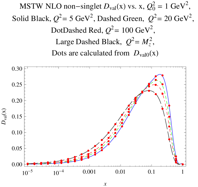
Figure 1: The NLO MSTW Martin et al. (2009) non-singlet valence distribution, $D_{\rm val}=x\left(d(x,Q^{2})-{\bar{d}}(x,Q^{2})\right)$, for $Q^{2}=5\ ,20,\ 100$ and $M_{z}^{2}$ GeV². The published MSTW Martin et al. (2009) curves are: $Q^{2}=5$ GeV², solid blue; $Q^{2}=20$ GeV², dashed green; $Q^{2}=100$ GeV², dot dashed red; $Q^{2}=M_{z}^{2}$ GeV², large dashed black. The dots are the evolution results for NLO non-singlet $D_{\rm val}=x\left(d(x,Q^{2})-{\bar{d}}(x,Q^{2})\right)$ from Eq. (57) (converted to $x$-space), using the NLO MSTW values for $F_{ns0}(x)$, where $Q^{2}_{0}=1$ GeV².

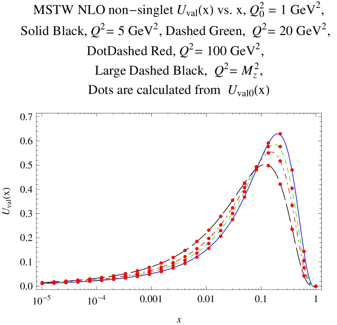
Figure 2: The NLO MSTW Martin et al. (2009) non-singlet valence distribution, $U_{\rm val}=x\left(u(x,Q^{2})-{\bar{u}}(x,Q^{2})\right)$, for $Q^{2}=5\ ,20,\ 100$ and $M_{z}^{2}$ GeV². The published MSTW Martin et al. (2009) curves are: $Q^{2}=5$ GeV², solid blue; $Q^{2}=20$ GeV², dashed green; $Q^{2}=100$ GeV², dot dashed red; $Q^{2}=M_{z}^{2}$ GeV², large dashed black. The dots are the evolution results for NLO non-singlet valence distribution, $U_{\rm val}=x\left(u(x,Q^{2})-{\bar{u}}(x,Q^{2})\right)$ from Eq. (57) (converted to $x$-space), using the NLO MSTW values for $F_{ns0}(x)$, where $Q^{2}_{0}=1$ GeV².

III.1.2 The NLO non-singlet $u$ quark valence distribution $U_{\rm val}=x\left(u(x,Q^{2})-{\bar{u}}(x,Q^{2})\right)$

In Fig. 2, we show the results obtained by evolving the non-singlet distribution valence distribution for the $u$ quark, $U_{\rm val}(x,Q^{2})=x\left(u(x,Q^{2})-{\bar{u}}(x,Q^{2})\right)$ from $Q_{0}^{2}=1$ GeV², for $Q^{2}=5\ ,20,\ 100$ and $M_{z}^{2}$ GeV². The published MSTW Martin et al. (2009) curves are: $Q^{2}=5$ GeV², solid blue; $Q^{2}=20$ GeV², dashed green; $Q^{2}=100$ GeV², dot dashed red; $Q^{2}=M_{z}^{2}$ GeV², large dashed black. The dots are our evolution results for NLO non-singlet $u$ quark valence distribution $U_{\rm val}(x,Q^{2})=x\left(u(x,Q^{2})-{\bar{u}}(x,Q^{2})\right)$ from Eq. (57) (converted to $x$-space), using the NLO MSTW values for $F_{ns0}(x)$, where $Q^{2}_{0}=1$ GeV². Again, the reproduction of the published MSTW data is excellent. The fractional errors at $x=0.135$, defined in Section III.1.1, are: frac. err. = -0.003 at $Q^{2}=5$ GeV² and frac. err. = +0.004 at $Q^{2}=M_{z}^{2}$ GeV².

IV Conclusions

For the singlet sector of pQCD, we have solved the coupled NLO DGLAP equations and found NLO decoupled analytic solutions for $F_{s}(x,Q^{2})$ and $G(x,Q^{2})$, an extension of our earlier work for LO Block et al. (2010). All that is required is knowledge of the initial distributions $F_{s0}(x)$ and G${}_{0}(x)$, at $Q^{2}=Q_{0}^{2}$, where $Q_{0}^{2}$ is the starting value for the evolution. For the non-singlet sector, we have successfully solved the NLO evolution equation for $F_{ns}(x,Q^{2})$, again in terms of $F_{ns0}(x)$, the value of $F_{ns}(x,Q^{2})$ at $Q_{0}^{2}$. We illustrated this numerically for NLO, calculating the non-singlet valence quark distributions $U_{\rm val}=x\left(u(x,Q^{2})-{\bar{u}}(x,Q^{2})\right)$ and $D_{\rm val}=x\left(d(x,Q^{2})-{\bar{d}}(x,Q^{2})\right)$ for a very large range of $x$ and $Q^{2}$, in excellent agreement with the NLO published MSTW Martin et al. (2009) values. We note that these techniques can be extended to arbitrary order in the strong coupling constant $\alpha_{s}(Q^{2})$, for both the singlet and non-singlet sector.

The results presented here are basically analytic, thus eliminating the need for simultaneous numerical solutions of the singlet and non-singlet DGLAP equations on a two-dimensional lattice in $x$ and $Q^{2}$. They provide new tools for studying pQCD; for example, they can be used to examine directly the sensitivity of an individual  evolved distribution to the assumed shapes of its starting distribution. In the future, we hope to apply these techniques to a global fit of experimental $F_{2}^{\gamma p}(x,Q^{2})$ data to determine in LO, a gluon starting distribution, and in NLO, approximate $F_{s}$ and gluon starting distributions. Since these starting distributions will be determined by experimental data, they will be free of predetermined shape hypotheses; this will allow us to find new gluon distributions that are critically needed for the interpretation of results from the Large Hadron Collider.

V Acknowledgments

The authors would like to thank the Aspen Center for Physics for its hospitality during the time parts of this work were done. P. Ha would like to thank Towson University Fisher College of Science and Mathematics for travel support. D.W.M. received travel support from DOE Grant No. DE-FG02-04AR41308.

References

- Block (2010a) M. M. Block, Eur. Phys. J. C 65, 1 (2010a).
- Block (2010b) M. M. Block, to be published (2010b), eprint arXiv:1004:3585[hep-ph].
- Martin et al. (2009) A. D. Martin, W. J. Stirling, R. S. Thorne, and G. Watt, Eur. Phys. J. C 63, 189 (2009), eprint arXiv:0901.0002 [hep-ph].
- Gribov and Lipatov (1972) V. N. Gribov and L. N. Lipatov, Sov. J. Nucl. Phys. 15, 438 (1972).
- Altarelli and Parisi (1977) G. Altarelli and G. Parisi, Nucl. Phys. B 126, 298 (1977).
- Dokshitzer (1977) Y. L. Dokshitzer, Sov. Phys. JETP 46, 641 (1977).
- Pumplin et al. (2002) J. Pumplin et al. (CTEQ), J. High Energy Phys. 0207, 012 (2002), eprint hep-ph/0201195.
- Tung et al. (2007) W. K. Tung, H. L. Lai, A. Belyaev, J. Pumplin, D. Stump, and C.-P. Yuan, J. High Energy Phys. 0702, 053 (2007), eprint hep-ph/0611254.
- Martin et al. (2002) A. D. Martin, R. G. Roberts, W. J. Stirling, and R. S. Thorne, Eur. Phys. J. C 23, 73 (2002), eprint hep-ph/0110215.
- Martin et al. (2004) A. D. Martin, R. G. Roberts, W. J. Stirling, and R. S. Thorne, Phys. Lett. B 604, 61 (2004), eprint hep-ph/0410230.
- Block et al. (2008) M. M. Block, L. Durand, and D. W. McKay, Phys. Rev. D 77, 094003 (2008), eprint arXiv:0710.3212 [hep-ph].
- Block et al. (2009) M. M. Block, L. Durand, and D. W. McKay, Phys. Rev. D 79, 014031 (2009), eprint arXiv:0808.0201 [hep-ph].
- Block et al. (2010) M. M. Block, L. Durand, P. Ha, and D. W. McKay, to be published (2010), eprint arXiv:1004.1440 [hep-ph].
- Mat (2009) Mathematica 7, a computing program from Wolfram Research, Inc., Champaign, IL, USA, www.wolfram.com (2009).