Natural Units For Nuclear Energy Density Functional Theory

Abstract

Naive dimensional analysis based on chiral effective theory, when adapted to nuclear energy density functionals, prescribes natural units and a hierarchy of contributions that could be used to constrain fits of generalized functionals. By applying these units, a large sample of Skyrme parametrizations is examined for naturalness, which is signaled by dimensionless coupling constants of order one. The bulk of the parameters are found to be natural, with an underlying scale consistent with other determinations. Significant deviations from unity are associated with deficiencies in the corresponding terms of particular functionals or with an incomplete optimization procedure.

Introduction. New experimental data for atomic nuclei throughout the nuclear mass chart are becoming available thanks to radioactive nuclear beam efforts worldwide. This is coupled with increasingly sophisticated theoretical descriptions of low-energy nuclear phenomena bluebook ; scidac . These developments drive higher requirements for the quality and predictive power of nuclear structure investigations.

Nuclear density functional theory (DFT) Bender03 is the only available theoretical tool for the microscopic description of nuclear properties that spans the full nuclear mass chart. The non-relativistic Skyrme energy density functional (EDF) is based on local nuclear densities and currents and is specified by a set of coupling constants. There are many sets of Skyrme parameters determined through different optimizations to experimental energies, radii, and other nuclear observables. After more than twenty years of experience, the standard Skyrme EDF has proved to be fairly successful in the overall description of experimental data. At the same time, its limitations have become well established, and the quest for better accuracy and stable predictive power motivates going beyond the standard Skyrme functional Carlsson:2008gm ; stoitsov-scidac .

New developments in nuclear DFT are inevitably associated with an optimization of EDF parameters to a selected set of experimental data. This is problematic if more general density dependencies and higher powers of gradients lead to an explosion of new parameters without control over their relative importance. A possible solution is to organize generalizations of the Skyrme functional by effective field theory principles that exploit the separation of scales and so establish a hierarchy of contributions. One such approach for low-energy quantum chromodynamics is naive dimensional analysis (NDA) for chiral effective field theory FRIAR96b , which has been adapted to relativistic nuclear EDFs with encouraging results FRIAR96 ; RUSNAK97 ; Furnstahl:2001un ; Burvenich:2001rh .

In the NDA approach, a scaling to “natural units” is applied to the functional, which if successful results in dimensionless parameters of order unity. This has practical benefits, because in numerical optimization it is advantageous to have all the parameters close to unity. But the use of natural units also provides guidance on maintaining a hierarchy and preventing fine tuning where higher orders play off against lower orders, particularly when linear combinations of the parameters are underdetermined.

The relevance of naturalness for Skyrme functionals was suggested long ago in Ref. Fur97 , but the resulting natural units have not been widely employed (or validated) by DFT practitioners. The first test was very limited in the range of functionals and focused on isoscalar parameters Fur97 . The goal of this paper is to investigate whether natural units apply more generally to existing Skyrme parameterizations, including the modern ones, and thereby motivate their use in future nuclear DFT developments. As part of this study, an online converter to natural units has been created at http://massexplorer.org, where one can browse and convert the Skyrme forces considered in this paper as well as try new sets of parameters to check whether they are natural.

Skyrme Energy Density Functional. The standard Skyrme energy density can be written in isospin representation as a sum of kinetic and potential isoscalar ($t=0$) and isovector ($t=1$) energy density terms

$${\cal H}(\bm{r})=\displaystyle\frac{\hbar^{2}}{2m}\tau_{0}+{\cal H}_{0}(\bm{r})+{\cal H}_{1}(\bm{r})\;,$$ (1)

where the time-even part is

$${\cal H}_{t}(\bm{r}) = \displaystyle\left(C_{t0}^{\rho}+C_{t{\rm D}}^{\rho}~{}\rho_{0}^{\gamma}\right)\rho_{t}^{2}+C_{t}^{\Delta\rho}\rho_{t}\Delta\rho_{t}+C_{t}^{\tau}\rho_{t}\tau_{t}$$ (2)

$$\hbox{}+\displaystyle\tfrac{1}{2}C_{t}^{J}\bm{J}_{t}^{2}+C_{t}^{\nabla J}\rho_{t}\bm{\nabla}\cdot\bm{J}_{t}\;,$$

The isospin index $t=\{0,1\}$ labels isoscalar and isovector densities $\rho_{t}$, $\tau_{t}$, and $\bm{J}_{t}$, respectively. The standard definitions of these local densities can be found in Ref. Perlinska04 . The energy density of Eq. (1) depends on 13 parameters; that is, 12 coupling constants and one exponent $\gamma$,

$$\{C_{t0}^{\rho},C_{t{\rm D}}^{\rho},C_{t}^{\Delta\rho},C_{t}^{\tau},C_{t}^{J},C_{t}^{\nabla J},\gamma\}\;,$$ (3)

which are typically obtained by adjusting the functional to produce certain properties in finite nuclei and/or in infinite nuclear matter. Historically, the Skyrme force and the Skyrme functional derived from it were defined by using the $\{t_{n},x_{n}\}$ parametrization. The link between these two representations can be found in Ref. Bender03 . The most general Skyrme functional also contains a time-odd part with associated time-odd coupling constants, which become relevant in nuclear states with nonzero angular momentum (e.g., odd-mass nuclei) Bender03 . In this work we consider only the time-even part and leave the time-odd coupling constants as a subject of future study.

Natural units. Following Ref. Fur97 , we scale the Skyrme coupling constants by analogy to an effective Lagrangian where each term is schematically written as

$$g\left[\frac{\psi^{{\dagger}}\psi}{\Lambda f_{\pi}^{2}}\right]^{l}\left[\frac{\nabla}{\Lambda}\right]^{n}\Lambda^{2}f_{\pi}^{2}\;,$$ (4)

with $g$ being a dimensionless coupling constant and $f_{\pi}\approx 93$ MeV is the pion decay constant. The momentum $\Lambda$ characterizes the breakdown scale of the chiral effective theory. As such, it is expected to be in the range $500\,\mbox{MeV}<\Lambda<1000\,\mbox{MeV}$. Naturalness implies that $g$ should be of order unity, which in practice roughly means between 1/3 and 3 (unless there is a symmetry reason making $g$ small). If natural, Eq. (4) implies a hierarchy of terms with a density expansion (powers of $l$) and a gradient expansion (powers of $n$) FRIAR96 ; RUSNAK97 ; Furnstahl:2001un ; Burvenich:2001rh ; Fur97 .

The conversion of the Skyrme couplings to natural units is accomplished in the present work by multiplying each by a scaling factor

$$S=f_{\pi}^{2(l-1)}\Lambda^{n+l-2}\;,$$ (5)

where $l$ is the power of densities in the corresponding term and $n$ is the number of derivatives for that term. In Ref. Fur97 only functionals with integer powers of the density-dependent term were considered. Here we generalize the scaling to include also fractional powers $\gamma$ used in Skyrme functionals by setting $l=2+\gamma$ for the density-dependent term. At present this is just a prescription. In studies of dilute fermion systems in a harmonic trap, it was shown that terms with fractional powers in a perturbative functional followed scaling rules Bhattacharyya:2004qm , but this has not yet been derived for the nuclear case.

We also generalize our analysis to the isovector coupling constants, which highlights the issue of possible additional numerical factors in the NDA prescription of Eqs. (4) and (5). A direct extension to the isovector channel scales the isovector coupling constants with the same scale factor $S$ as the corresponding isoscalar couplings. However, in past applications of the NDA to relativistic meson and point coupling models, the isovector prescription included an additional factor of four. This arises from the construction of the Noether current for an isospin transformation, which in the conventional normalization has a 1/2 with each $\tau$ matrix (so that $[T_{a},T_{b}]=i\epsilon_{abc}T_{c}$ implies $T_{a}=\tau_{a}/2)$. Then the isovector current is $1/2\overline{\psi}\gamma^{\mu}\tau\psi$ and so $1/2(\rho_{p}-\rho_{n})$ is the corresponding charge density used in the naturalness analysis. Although this may be no more than a theoretical prejudice, the empirical observation in other NDA tests was that the scaled constants consistently came out closer to unity Furnstahl:1999rm . In the present study we consider both isovector scalings.

More generally, to decide on possible additional numerical factors we rely on the correspondence of Skyrme EDF terms to those from a non-relativistic reduction of a relativistic formulation (e.g., meson exchange with masses of order $\Lambda$). For example, one might wonder if the spin-matrix $\sigma$ should lead to extra scaling factors between scalar terms and those involving the vector densities ${\bm{J}}_{t}$. We find that such terms arise with the same relative factor as terms with $\rho\tau$ and so we scale them the same.

For all coupling constants entering the standard functional of Eqs. (1) and (2), one has $l=2$ except for the density-dependent constant $C_{t{\rm D}}^{\rho}$, for which $l=2+\gamma$. Similarly, the power is $n=0$ for $C_{t}^{\rho}$, while for all other constants $n=2$. In this way, scaling all coupling constants $C^{\sigma}_{t}$ with the associated factors $S^{\sigma}$, $\sigma=\{\rho,\Delta\rho,\tau,\nabla J\}$ yields dimensionless constants $S^{\sigma}C^{\sigma}_{t}$. The small ranges for $l$ and $n$ preclude testing the fine details of the NDA scaling hypothesis. However, by making a global analysis of Skyrme parametrizations, we can check for consistency, for trends and exceptions to naturalness, and for a preferred range of $\Lambda$. When parameter sets for extended functionals that include higher-order derivatives Carlsson:2008gm and/or higher powers of density Biruk are available, more definitive tests of natural scaling will be possible.

The list of functionals considered is given in Table 1. In this table we also categorize the functionals based on the strategy used to determine the couplings.

Table 1: List of Skyrme functionals and categories used in this study. The categories are: a) masses of double-magic nuclei (includes ⁹⁰Zr, ¹¹⁶Sn, ¹²⁴Sn, and ¹⁴⁰Ce) used in the fit; b) masses of non-double-magic nuclei used in the fit; c) charge radii used in the fit; d) single-particle energies used in the fit; e) symmetric infinite nuclear matter constrains considered in the fit; f) asymmetric infinite nuclear matter constrains considered in the fit; g) surface properties (neutron skin, fission barriers, etc.) considered in the fit; h) pairing was present in the fit; i) some parameters were fixed in the fit; j) parameters extrapolated or fine-tuned from an existing force or functional.

Index	Functionals	Categories	Ref
1–2	SkT3, SkT6	a d i j	SKT1-9
3	SkM	a c e f g i	SKM
4	SkM*	g j	SKMS
5–6	SGI, SGII	d e j	SGI-II
7	HFB9	a b f h i	HFB9
8–9	SI, SII	a c d e f i	SI-II
10	SkA	a c d e g i j	SKA
11	HFB16	a b c f h i	HFB16
12	SkT	a b d e g h i	SKT
13–16	SLy4–7	a c d e f i	SLY4-7
17–18	SkI1–2	a b c d f g i	SKI1-5
19–20	SkI3–4	a b c d f g i	SKI1-5
21	SkI5	a b c d f g i	SKI1-5
22–27	MSk1–6	a b f h i	MSK1-6
28–29	SIII, SIV	a c i	SIII-VI
30–31	SV, SVI	a c i j	SIII-VI
32–33	SLy230a,b	a c d e f i	SLY230A-B
34–39	E, Eσ, Z, Zσ, Rσ, Gσ	a c d g i	E-GSIGMA
40	SkP	a b c e f h i	SKP
41–42	SkO,SkO’	a b c d f g i	SKO-P
43	SV-min	a b c d g h	SVMIN
44	SkO${}_{T^{\prime\prime}}$	i j	SKOTPP
45	SkMP	a j	SKMP
46–47	SkX, SkXc	a b c d e f	SKX-C
48	RATP	a d e f i	RATP

The test of whether we truly have natural units is whether $S^{\sigma}$ makes the values of all scaled constants $S^{\sigma}C^{\sigma}_{t}$ of order unity. Their numerical values will obviously depend on the value of the cut-off parameter $\Lambda$ Fur97 . In our global study, the naturalness criterion can itself be used to extract the value of $\Lambda$ by minimizing the deviation of the coupling constants from unity. We consider a logarithmic root-mean-square deviation (RMSD)

$${\rm RMSD}=\sqrt{\frac{1}{N}\sum_{i,\sigma,t}\log_{10}^{2}|C^{\sigma}_{t}(i)|},$$ (6)

because naturalness implies couplings should not be too small as well as not too large. If a particular coupling constant is zero, it is excluded from the logarithmic RMSD.

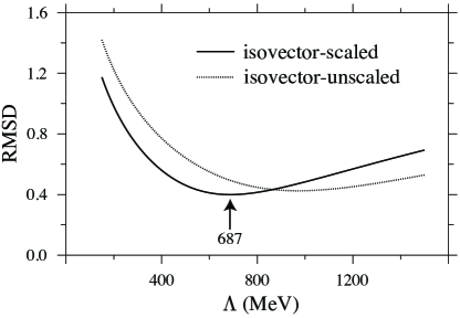
Figure 1: Logarithmic RMSD as a function of $\Lambda$ with (scaled) and without (unscaled) an extra factor of four for isovector terms. See text for details.

In Fig. 1 we plot RMSD for 48 EDFs as a function of $\Lambda$ with (scaled) and without (unscaled) the extra factor of four for isovector terms. It can be seen that the two different scalings produce different optimal $\Lambda$ with the scaled result yielding a clearer minimum that is numerically more consistent with studies of relativistic functionals. However, the minima in the RMSD curves are quite shallow, so $\Lambda$ cannot be considered to be sharply determined for the present Skyrme functionals.

In the present study, we choose to use the scaled isovector coupling constants for which the optimum is $\Lambda=687$ MeV (but the precise value does not affect our conclusions). In Fig. 2 we have plotted the scaled coupling constants for all the functionals of Table 1. Also, we plot the square-roots of individual RMSD contributions given by the functional to the total RMSD value. It can be seen that the Skyrme functionals have almost all of their parameter values in the interval $(1/3,3)$ with the bulk between $1/2$ and 2. Exceptions are discussed below.

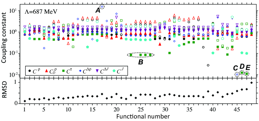
Figure 2: (color online) Scaled coupling constants $|C^{\sigma}_{t}|$ at $\Lambda=$687 MeV (top) and contributions of individual functionals to the total RMS value (bottom). The filled symbols refer to the isoscalar coupling constants and empty symbols to the isovector ones. The ordering of functionals by index is the same as in Table 1.

We also make a comparison between different representations of two particular functionals: SIII and HFB16. The parameters of these functionals are listed in Table 2 first by using the $(t,x)$-parametrization and then by the natural units parametrization, obtained from the corresponding coupling constants. As can be seen, in the $(t,x)$-parametrization these two functionals seem to be quite different from each other. However, when expressed in natural units the coupling constants of SIII and HFB16 are order unity. In Table 2 we also list in natural units the average, minimum, and maximum value for each coupling constant found in the set of 48 functionals. This information may provide useful insights into the expected values and ranges of coupling constants for future attempts to fit new functionals.

Table 2: Comparison between the SIII and HFB16 functionals in the $(t,x)$-parametrization and using natural units. We also list for each coupling constant the average, minimum, and maximum value found in the set of 48 functionals. In all cases, $\Lambda=687\,$MeV was used.

$(t,x)$-parameters			Couplings in natural units
	SIII	HFB16		SIII	HFB16	Average	Min.	Max.
$t_{0}$	$-$1128.75	$-$1837.23	$C^{\rho}_{00}$	$-$0.4767	$-$0.7759	$-$0.7977	$-$1.2380	$-$0.4465
$t_{1}$	395.0	383.521	$C^{\rho}_{10}$	1.2076	1.9295	1.7656	$-$0.9795	4.5761
$t_{2}$	$-$95.0	$-$3.41736	$C^{\rho}_{0{\rm D}}$	0.7623	0.7509	0.7824	0.2723	1.2616
$t_{3}$	14000.0	11523.0	$C^{\rho}_{1{\rm D}}$	$-$3.0493	$-$2.3825	$-$2.2010	$-$6.0116	1.9790
$x_{0}$	0.45	0.432600	$C^{\tau}_{0}$	0.6059	0.4464	0.5606	$-$0.0856	2.9421
$x_{1}$	0	$-$0.824106	$C^{\tau}_{1}$	$-$1.6726	$-$0.2048	$-$0.3626	$-$2.9469	3.5160
$x_{2}$	0	44.6520	$C^{\Delta\rho}_{0}$	$-$0.8597	$-$0.8702	$-$0.8765	$-$1.7491	$-$0.4636
$x_{3}$	0	0.689797	$C^{\Delta\rho}_{1}$	0.9301	$-$0.8998	$-$0.5531	$-$15.5202	2.5762
$W_{0}$	120.0	141.100	$C^{\nabla J}_{0}$	$-$1.2288	$-$1.4449	$-$1.2385	$-$1.6384	$-$0.8957
			$C^{\nabla J}_{1}$	$-$1.6384	$-$1.9265	$-$1.0875	$-$2.1846	5.4272
			$C^{J}_{0}$	0	1.1300	0.5159	$-$0.6021	1.4212
			$C^{J}_{1}$	0	1.3208	1.6502	$-$5.0026	3.6049

Deviations from order unity. The deviations of the coupling constants $C^{\sigma}_{t}$ from unity are illustrated in the summary plot in Fig. 2. As noted earlier, almost all parameters are found to lie within the interval of $(1/3,3)$. In terms of naturalness, we do not observe any significant differences between the functionals that are strictly based on the Skyrme force and the extended functionals. However, significant deviations still exist for some particular Skyrme functionals for the coupling constants $C_{0}^{J},C_{1}^{\Delta\rho}$, and $C_{0}^{\Delta J}$, and more generally for $C^{\rho}_{1{\rm D}}$, which appears borderline unnaturally large in many cases. If we accept that nuclear functionals are characterized by naturalness, such deviations could indicate some deficiency in the associated term of the functional or they could simply reflect a specific strategy applied to the optimization procedure.

While in some cases no definite cause has been identified, we can identify various examples of unnatural couplings that do have probable explanations. For example, it is well known that tensor terms are rather poorly constrained by the experimental data; most Skyrme functionals do not include tensor terms at all. The significant deviations seen in Fig. 2 for the $C_{0}^{J}$ parameters most likely reflects this situation.

Another instructive example is the deviation for $C_{1}^{\Delta\rho}$ in the case of SkI1 (case A in Fig. 2). The optimization of SkI1 excluded the isotope shift data while all other SkI forces (SkI2–SkI5) consider these data. This isotopic shift data contains the charge radii difference between ⁴⁰Ca and ⁴⁸Ca, and ²⁰⁸Pb and ²¹⁴Pb. All SkI functionals are, however, optimized by using diffraction radii data, which is closely related to charge radii.

The deviation in $C_{0}^{\tau}$ for SV results from an artificially imposed vanishing density-dependent term, which results in a too-low isoscalar effective mass (0.38). The EDF RATP demonstrates a clear example of an anomalously small $C^{\Delta\rho}_{1}\approx-0.0019$ (not seen on the scale of Fig. 2). This can probably be attributed to the fitting procedure, where the focus was mainly on infinite nuclear matter properties for astrophysical applications. Similarly, $C^{\Delta\rho}_{1}$ of SkMP (case C) is also very small. This can be linked to the fact that this functional was obtained by mixing $t$- and $x$-parameters of SkM* and SkP functional and making small adjustments to the volume part of the functionals. Therefore, almost no attention was paid to the surface part either in RATP or SkMP functionals.

Another example is an anomalously small $C_{0}^{\tau}$, found in SkX and SkX_c (cases D and E). This is due to the fact that in fitting these forces, much emphasis was put on the single-particle energies. This leads to an effective mass close to one, and therefore a small coupling constant. Similarly, in the MSk series (case B) the fit favored effective mass close to one, and it was therefore set by hand either to 1.0 or 1.05. This, however, does not imply that single-particle energies are not suitable observables in the fitting procedure.

Finally, the seemingly unnaturally large $C^{\rho}_{1{\rm D}}$ couplings may reflect an inadequate treatment of terms with fractional density dependence. Alternatively, the fact that the isovector $C^{\rho}_{10}$ couplings are also sometimes unnatural hints at a problem with the scaling of terms associated with pion-range physics. The density matrix expansion applied to the leading long-range contributions from chiral effective field theory may shed light on this issue.

These examples illustrate that the use of natural units in nuclear DFT not only introduces the simplicity of dimensionless coupling constants and the convenience of their order-unity values, but also can give valuable pointers to potential deficiencies of the physics invoked when constructing and optimizing the functional.

Conclusions. In this study, the coupling constants of a large set of Skyrme EDFs have been examined for naturalness as an extension of Ref. Fur97 . While the limited range of density and gradient terms in the standard Skyrme parameterizations means that a definitive test of NDA chiral naturalness is not possible, the best functionals are consistent with naturalness and a scale $\Lambda$ of about 700 MeV. Significant deviations from unity can be associated with deficiencies in fitting the functional or with specific optimization procedures. This motivates using naturalness as a guiding principle for constructing new generalized Skyrme functionals. An online natural units convertor has been set up at http://massexplorer.org as a tool for such applications. Further investigation is needed to better understand how to treat non-analytic density dependence and hybrid functionals where the density matrix expansion is used for long-range contributions. Finally, we note that the phenomenologically successful finite-range Gogny functionals can be accommodated within the Skyrme framework Dobaczewski:2010qp , which can be used to broaden the application of natural units.

The UNEDF SciDAC Collaboration is supported by the Office of Nuclear Physics, U.S. Department of Energy under Contracts Nos. DE-FC02-09ER41583 and DE-FC02-09ER41586 (UNEDF SciDAC Collaboration), DE-FG02-96ER40963 (University of Tennessee), and by the National Science Foundation under Grant No. PHY–0653312. Computational resources were provided by the National Center for Computational Sciences at Oak Ridge and the National Energy Research Scientific Computing Facility.

References

- (1) RIA Theory Bluebook: A Road Map, http://fribusers.org.
- (2) G.F. Bertsch, D.J. Dean, and W. Nazarewicz, SciDAC Review 6, Winter 2007, p. 42.
- (3) M. Bender, P.-H. Heenen, and P.-G. Reinhard, Rev. Mod. Phys. 75, 121 (2003).
- (4) B.G. Carlsson, J. Dobaczewski, and M. Kortelainen, Phys. Rev. C 78, 044326 (2008) [Erratum-ibid. C 81, 029904 (2010)].
- (5) M. Stoitsov et al., J. Phys.: Conf. Ser. 180, 012082 (2009).
- (6) J.L. Friar, Few Body Syst. 22, 161 (1997).
- (7) J.L. Friar, D.G. Madland, and B.W. Lynn, Phys. Rev. C 53, 3085 (1996).
- (8) J.J. Rusnak and R.J. Furnstahl, Nucl. Phys. A 627, 495 (1997).
- (9) R.J. Furnstahl, Nucl. Phys. A 706, 85 (2002).
- (10) T. Burvenich, D.G. Madland, J.A. Maruhn, and P.G. Reinhard, Phys. Rev. C 65, 044308 (2002).
- (11) R.J. Furnstahl and James C. Hackworth, Phys. Rev. C 56, 2875 (1997).
- (12) E. Perlińska et al., Phys. Rev. C 69, 014316 (2004).
- (13) A. Bhattacharyya and R.J. Furnstahl, Nucl. Phys. A 747, 268 (2005).
- (14) R.J. Furnstahl and B.D. Serot, Nucl. Phys. A 671, 447 (2000).
- (15) B. Gebremariam, S.K. Bogner, and T. Duguet, arXiv:1003.5210.
- (16) F. Tondeur et al., Nucl. Phys. A 420, 297 (1984).
- (17) H. Krivine, J. Treiner, and O. Bohigas, Nucl. Phys. A 336, 155 (1980).
- (18) J. Bartel et al., Nucl. Phys. A 386, 79 (1982).
- (19) Nguyen Van Giai, H. Sagawa, Phys. Lett. B 106, 379 (1981).
- (20) S. Goriely et al., Nucl. Phys. A 750, 425 (2005).
- (21) D. Vautherin and D.M. Brink, Phys. Rev. C 5, 626 (1972).
- (22) H.S. Köhler, Nucl. Phys. A 258, 301 (1976).
- (23) N. Chamel, S. Goriely, and J.M. Pearson, Nucl. Phys. A 812, 72 (2008).
- (24) F. Tondeur, Phys. Lett. B 123, 139 (1983).
- (25) E. Chabanat et al., Nucl. Phys. A 635, 231 (1998).
- (26) P.-G. Reinhard and H. Flocard, Nucl. Phys. A 584, 467 (1995)
- (27) F. Tondeur et al., Phys. Rev. C 62, 024308 (2000).
- (28) M. Beiner et al., Nucl. Phys. A 238, 29 (1975).
- (29) E. Chabanat et al., Nucl. Phys. A 627, 710 (1997).
- (30) J. Friedrich and P.-G. Reinhard, Phys. Rev. C 33, 335 (1986).
- (31) J. Dobaczewski, H. Flocard, and J. Treiner, Nucl. Phys. A 422, 103 (1984).
- (32) P.-G. Reinhard et al., Phys. Rev. C 60, 014316 (1999).
- (33) P. Klüpfel et al., Phys. Rev. C 79, 034310 (2009).
- (34) M. Zalewski et al., Phys. Rev. C 80, 064307 (2009).
- (35) L. Bennour et al., Phys. Rev. C 40, 2834 (1989).
- (36) B.A. Brown, Phys. Rev. C 58, 220 (1998).
- (37) M. Rayet et al., Astron. Astrophys. 116, 460 (1982).
- (38) J. Dobaczewski, B.G. Carlsson, and M. Kortelainen, J. Phys. G: Nucl. Part. Phys. 37, 075106 (2010).