Dehydration and ionic conductance quantization in nanopores

Abstract

There has been tremendous experimental progress in the last decade in identifying the structure and function of biological pores (ion channels) and fabricating synthetic pores. Despite this progress, many questions still remain about the mechanisms and universal features of ionic transport in these systems. In this paper, we examine the use of nanopores to probe ion transport and to construct functional nanoscale devices. Specifically, we focus on the newly predicted phenomenon of quantized ionic conductance in nanopores as a function of the effective pore radius - a prediction that yields a particularly transparent way to probe the contribution of dehydration to ionic transport. We study the role of ionic species in the formation of hydration layers inside and outside of pores. We find that the ion type plays only a minor role in the radial positions of the predicted steps in the ion conductance. However, ions with higher valency form stronger hydration shells, and thus, provide even more pronounced, and therefore, more easily detected, drops in the ionic current. Measuring this phenomenon directly, or from the resulting noise, with synthetic nanopores would provide evidence of the deviation from macroscopic (continuum) dielectric behavior due to microscopic features at the nanoscale and may shed light on the behavior of ions in more complex biological channels.

I Introduction

The behavior of water and ions confined in nanoscale geometries is of tremendous scientific interest. On the one hand, biological ion channels, which form from membrane proteins, perform crucial functions in the cell Hille01-1 ; Ashcroft00-1 . On the other hand, there have been recent advances in aqueous nanotechnology such as nanopores and nanochannels, which hold great promise as the basic building blocks of molecular sensors, ultra-fast DNA sequencers, and probes of physical processes at the nanoscale Zwolak08-1 . Indeed, nanopore-based proposals for DNA sequencing range from measuring transverse electronic currents driven across DNA Zwolak05-1 ; Lagerqvist06-1 ; Lagerqvist07-1 ; Lagerqvist07-2 ; Krems09-1 to voltage fluctuations of a capacitor Heng2005-1 ; Gracheva2006-1 ; Gracheva2006-2 to ionic currents Kasianowicz1996-1 ; Akeson1999-1 ; Deamer2000-1 ; Vercoutere2001-1 ; Deamer2002-1 ; Vercoutere2002-1 ; Vercoutere2003-1 ; Winters-Hilt2003-1 .

Recent experiments show that we are tantalizingly close to realizing a device capable of ultra-fast, single-molecule DNA sequencing with nanopores: identification of individual nucleotides using transverse electronic transport Tsutsui10-1 ; Chang10-1 has been demonstrated. Discrimination of nucleotides using their ionic blockade current when driving them individually though a modified biological pore has also been demonstrated Clarke09-1 ; Stoddart09-1 . In these systems, the presence of water and ions will affect the signals and noise measured and thus understanding their behavior is an important issue in both science and technology.

Many computational studies have been dedicated to relating the three-dimensional structure Doyle98-1 ; Hille01-1 ; Chung07-1 of biological ion channels to their physiological function, e.g., ion selectivity. For instance, recent studies have examined the role of ligand coordination in potassium selective ion channels Thomas07-1 ; Varma07-1 ; Fowler08-1 ; Dudev09-1 . Biological channels, however, are complex pores with many potential factors contributing to their operation. Thus, only in a limited number of cases have universal mechanisms of ion transport been investigated, such as the recent work on the role of “topological constraints” in ligand coordination Bostick07-1 ; Yu09-1 ; Bostick09-1 .

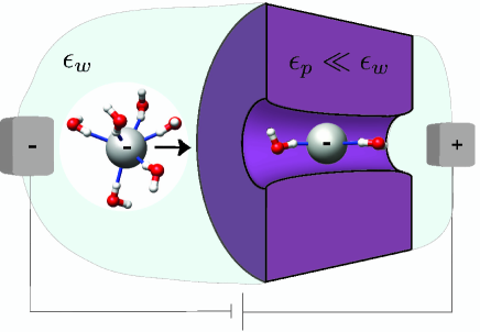
Figure 1: Schematic of ion transport in the presence of hydration layers. Only the first hydration layer is shown for simplicity. Ions in bulk water form hydration layers that make the ion behave as a “quasi-particle” that includes the ion and tightly bound water molecules. This quasi-particle is then solvated in the high-dielectric water. As the ion goes from the bulk solution to the pore it has to partially shed its hydration layers, i.e., the quasi-particle has to break apart. This gives a nonlinearity in the energetic barrier to transport. A continuum picture neglects these features and considers only the dielectric barrier that ions have to overcome by moving from bulk water with dielectric constant $\epsilon_{w}$ into the inhomogeneous, low-dielectric pore environment with $\epsilon_{p}\ll\epsilon_{w}$. Specialized proteins facilitate this process in biological ion channels via the presence of localized surface charges/dipoles and other mechanisms.

Fundamental developments in the fabrication of synthetic nanopores Li2001-1 ; Miller01-1 ; Storm2003-1 ; Holt04-1 ; Siwy04-1 ; Harrell04-1 ; Holt06-1 ; Dekker07-1 , however, open new venues for investigating the behavior of ion channels and dynamical phenomena of ions, (bio-)molecules, and water at the nanoscale. For instance, what are the dominant mechanisms determining ionic currents and selectivity? What role do binding sites play versus hydration in constrained geometries? How accurate are “equilibrium” and/or continuum theories of ion transport? Well-controlled synthetic pores can be used in this context to examine how ion transport is affected, for instance, by changing only the pore radius, in the absence of binding sites and significant surface charge within the pore.

In this paper we examine the role of dehydration in ionic transport through nanopores. In particular, we investigate the recent prediction of quantized ionic conductance by two of the present authors (MZ and MD) Zwolak09-1 , namely that drops in the conductance, as a function of the effective pore radius, should occur when successive hydration layers are prevented from entering the pore. This effect is a classical counterpart of the electronic quantized conductance one observes in quantum point contacts as a function of their cross section (see, e.g., Ref. Diventra2008-1 ). We examine different ions, both positive and negative, and of different valency (namely, $\mathrm{Cl}^{-}$, $\mathrm{Na}^{+}$, $\mathrm{K}^{+}$, $\mathrm{Ca}^{2+}$, and $\mathrm{Mg}^{2+}$). We find that the ion type plays only a minor role in the radii of the hydration layers, and thus does not affect much the pore radii at which a sudden drop in the current is expected. Divalent ions, however, are the most ideal experimental candidates for observing quantized ionic conductance because of their more strongly bound hydration layers. Further, the fluctuating hydration layer structure and changing contents of the pore should give a peak (versus the effective pore radius) in the relative current noise - giving an additional method to observe the effect of the hydration layers. Thus, we elucidate how quantized ionic conductance provides a novel tool to deconstruct the energetic contributions to ion transport.

The paper is organized as follows: In Sec. II, we give a macroscopic (i.e., a continuum electrostatic) viewpoint on the energetics of ion transport. In Sec. III, we examine how ions induce local structures in the surrounding water known as hydration layers - an effect that is not taken into account when using continuum electrostatics to estimate energetic barriers to transport. Further, we calculate the energies stored in these layers and develop a model for the energetic barrier for ions entering a pore. In Sec. IV, we use a Nernst-Planck approach to relate this barrier to the ionic current. In Sec. V, we discuss how the presence of the hydration layers gives rise to a peak in the relative noise in the ionic current at values of the effective pore radius congruent with a layer radius. In Sec. VI, we then present our conclusions.

II Ionic Transport

The experimental set-up we are interested in is that of ions driven through a pore/channel of nanoscale dimensions under the action of a static electric field . Such a situation is depicted in Fig. 1. A simple approach to ionic transport is to envision the ions moving through an energetic barrier due to going from the high-dielectric aqueous environment into the inhomogeneous, low-dielectric environment of the pore, treating the surroundings as continuum media. The resulting approach is inherently static: by analyzing the energetic barrier to (near-equilibrium) transport one obtains information about how different factors - the pore material (through its dielectric constant), the pore dimensions, the presence of surface charges, and the presence of the high-dielectric water along the pore axis - would affect transport.

Indeed, one of the first calculations of the dielectric barrier (using a “Born solvation” model) was done by considering the ion solvated in water and moved into a low-dielectric, pore-less membrane Parsegian69-1 ; Parsegian75-1 . This provides an estimate of the energies involved by calculating the energy change of solvating the ion in continuum water, with dielectric constant $\epsilon_{w}\approx 80$, to “solvating” it in a continuum material with $\epsilon_{p}\approx 2$ (representative of lipid membranes ). For instance, the energy change of a $\mathrm{Cl}^{-}$ ion, with effective radius $R\approx 2\,\textrm{\AA}$ , moved from continuum water to the continuum material is

$$\Delta U = \frac{e^{2}}{8\pi R\epsilon_{0}}\left(\frac{1}{\epsilon_{p}}-\frac{1}{\epsilon_{w}}\right)$$ (1)

$$\approx 1.8\,\mathrm{eV}.$$ (2)

This is quite a substantial energy change - about half the solvation free energy of $\mathrm{Cl}^{-}$ Hille01-1 ; Marcus91-1 . The finite thickness of the membrane does not change this value significantly. For thick membranes, it is lowered by Parsegian69-1 ; Parsegian75-1

$$\frac{e^{2}}{4\pi\epsilon_{0}\epsilon_{p}l}\ln\left(\frac{2\epsilon_{w}}{\epsilon_{w}+\epsilon_{p}}\right),$$ (3)

for $\epsilon_{w}\gg\epsilon_{p}$, where $l$ is the membrane thickness (and pore length). For $\epsilon_{p}\approx 2$ and $\epsilon_{w}\approx 80$, this gives $\sim 5/l\,\mathrm{eV}\,\textrm{\AA}\approx 0.1\,\mathrm{eV}$ for a membrane of thickness $l=50\,\textrm{\AA}$. That is, the Born estimate in Eq. (1) is lowered to $\sim 1.7\,\mathrm{eV}$. However, the membrane width Levitt78-1 and composition can play a significant role in this estimate. For the common synthetic pores made of silicon dioxide ($\epsilon_{p}\approx 4$) or silicon nitride ($\epsilon_{p}\approx 7.5$) the estimate in Eq. (1) is reduced from $\sim 1.8\,\mathrm{eV}$ to $\sim 0.9\,\mathrm{eV}$ and $\sim 0.4\,\mathrm{eV}$, respectively. These barriers are more than an order of magnitude larger than $k_{B}T$ at room temperature, where $k_{B}$ is the Boltzmann constant.

Due to this magnitude, it is clear that the energy scale of solvation is one of the controlling factors in ion transport. However, in addition to the above there is water present in the pore. One expects, therefore, that the energy of solvation would be decreased from simple estimates like that of Eq. (1). Several groups have calculated this contribution Parsegian69-1 ; Parsegian75-1 ; Levitt78-1 ; Jordan81-1 ; Jordan82-1 . For instance, Ref. Roux04-1 shows that the energy barrier of bringing an ion from continuum water into a low-dielectric, continuum membrane is reduced from $\sim 40\,\mathrm{kcal/mol}\approx 1.7\,\mathrm{eV}$ to $\sim 20\,\mathrm{kcal/mol}\approx 0.9\,\mathrm{eV}$ by the presence of water in the pore. This demonstrates that a pore filled with a high dielectric medium (e.g., continuum water) can significantly lower the barrier to transport. Even still, the barrier remains substantial.

In biological systems, however, the pores provide a channel with a much lower barrier as indicated by the conductance of many biological ion channels. These pores are formed from specialized proteins whose role is precisely to facilitate passage of ions (and further to selectively allow passage of certain ions). Clearly, pores with internal charges and/or dipoles can significantly reduce the energetic barriers for transport. Indeed, the effect of surface charges has been calculated in clean pores Teber2005-1 ; Zhang2005-1 ; Kamenev2006-1 and when present in sufficient amounts would negate the effect we predict as the reduction of the energetic barrier would be comparable to, or larger than, the hydration layer energies. Therefore, our interest is in clean pores with little to no surface charge where clear-cut experiments can be performed to understand the effect of hydration on transport. This rules out the direct use of some biological ion channels, particularly those with very small pores where single-file transport occurs Finkelstein81-1 ; Doyle98-1 ; Morais01-1 , because of the presence of localized charges and dipoles.

To conclude this section, we note that the continuum description suffers from a number of issues at the nanoscale: it is only valid beyond the correlation length of the material JacksonWater , which for the strong fields around an ion is $\sim 8\,\textrm{\AA}$ for water (see below), similar to the $\sim 5-8\,\textrm{\AA}$ in water only Narten72-1 ; linear continuum electrostatics is only valid when the polarization field is co-linear with the electric field (not the case in the hydration layers we discuss below); in a related issue, it is only valid for weak fields (in the context of ion channels, see, for example, Sec. 3.4 in Ref. Roux04-1 ); there is also an issue of where the “surface” separating the charge and the dielectric membrane/continuum water is located, especially for fluctuating atomic ensembles as is the case for protein pores and molecular (rather than continuum) water. Thus, while a continuum picture can highlight some general features of the energetic barrier to ion transport - in some cases giving compact analytical expressions - it breaks down when trying to understand the effect of structure at the nanoscale. In fact, macroscopic, continuum electrostatics is not designed to study specific features or short-range interactions at these length scales. This is precisely what we seek to address in the following sections.

III Hydration of Ions

We begin our study of quantized conductance by first illustrating how ions are hydrated in solution and then discuss the energies involved in this process. The formation of hydration layers around ions has been known for some time (see, e.g., Ref. Hille01-1 ), and is due to the strong local electric field around the ion and to repulsive short-range interactions among molecular/atomic species. We use molecular dynamics (NAMD2 Phillips05-1 ) simulations to understand the structure of hydration layers when different ions are inside and outside of nanopores .

Figures 2 and 3 show the water density oscillations for several common ionic species . There is a strong peak in water density about $3\,\textrm{\AA}$ away from the ions, with two further oscillations after that spaced about $2\,\textrm{\AA}$ apart. These oscillations signify that there are strongly bound water molecules forming around the ions. Table 1 lists the hydration layer radii from both this study and experiment. We find very good agreement with the experimental data for all cases. The water density approaches the bulk value ($\sim 0.033\,\mathrm{Molecules}/\textrm{\AA}^{3}$) at about $10\,\textrm{\AA}$, which is also consistent with the experimental value.

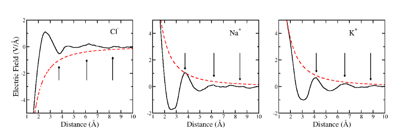
Figure 2: Top panels: Water density oscillations versus distance for $\mathrm{Cl}^{-}$, $\mathrm{Na}^{+}$, and $\mathrm{K}^{+}$ in bulk water. Black, solid lines indicate the density calculated from the oxygen atom positions for $\mathrm{Cl}^{-}$ and hydrogen atom positions for the cations. The arrows indicate the minimum in the density oscillations. The blue, dashed lines indicate the density calculated from the hydrogen atom positions for $\mathrm{Cl}^{-}$ and oxygen atom positions for the cations. Bottom panels: The electric field due to both the bare ion (red, dashed line) and due to the ion plus partial charges on the water molecules (black, solid). The arrows again indicate the minimum in the density oscillations.

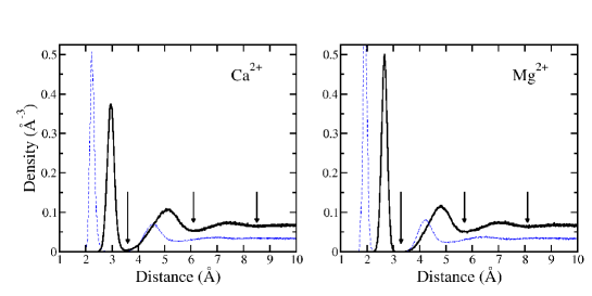
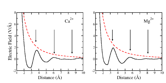
Figure 3: Top panels: Water density oscillations versus distance for $\mathrm{Ca}^{2+}$ and $\mathrm{Mg}^{2+}$ in bulk water. Black, solid lines indicate the density calculated from the hydrogen atom positions. The arrows indicate the minimum in the density oscillations. The blue, dashed lines indicate the density calculated from the oxygen atom positions. Bottom panels: The electric field due to both the bare ion (red, dashed line) and due to the ion plus partial charges on the water molecules (black, solid). The arrows again indicate the minimum in the density oscillations.

Ion	$R_{i}$ (Å) (th)	$R_{XO}$ (Å) (th)	$R_{XO}$ (Å) (exp)	$R_{I},R_{O}$ (Å)	$-U_{i}$ ($\mathrm{eV}$) (th)	$-\Delta G$ ($\mathrm{eV}$) (exp)	$\mu$ ($\mathrm{m}^{2}V/s$) (exp)
$\mathrm{Cl}^{-}$	3.1, 4.9, 7.1	3.1	3.19	2.0, 3.9, 6.2, 8.5	1.73, 0.68, 0.31	3.54	$7.92\times 10^{-8}$
$\mathrm{Na}^{+}$	2.9, 5.1, 7.5	2.3	2.44	1.9, 3.8, 6.2, 8.4	1.51, 0.72, 0.30	3.80	$5.19\times 10^{-8}$
$\mathrm{K}^{+}$	3.3, 5.6, 7.8	2.7	2.81	2.4, 4.2, 6.6, 8.8	1.15, 0.61, 0.27	3.07	$7.62\times 10^{-8}$
$\mathrm{Ca}^{2+}$	3.0, 5.1, 7.5	2.2, 4.6	2.42, 4.55	1.8, 3.6, 6.1, 8.5	7.89, 3.23, 1.32	15.65	$6.17\times 10^{-8}$
$\mathrm{Mg}^{2+}$	2.7, 4.8, 7.1	1.9, 4.2	2.09, 4.20	1.5, 3.3, 5.7, 8.1	10.33, 3.62, 1.48	19.03	$5.5\times 10^{-8}$

Table 1: Table of physical quantities from simulation and experiment. The theoretical hydration layer radii, $R_{i}$, for all three layers are defined using the ion-oxygen distance for $\mathrm{Cl}^{-}$ and ion-hydrogen distance for the cations. The first oxygen density maximum, $R_{XO}$, is for all ions $X$ using the present theory and experiment (average values taken from Ref. Ohtaki93-1 ). The second maximum is also shown for the divalent ions from both theory and experiment. The inner/outer radii that enter Eq. (4) are shown, the first of which is calculated such that Eq. (4) equals $\Delta G$ (exp) when $R_{i\nu}^{O}\rightarrow\infty$ (see also text). The next three inner/outer radii are taken from the minima of the oxygen density for $\mathrm{Cl}^{-}$ and the minima of the hydrogen density for the cations. Further, we report the layer energies $U_{i}$ (using $\epsilon_{p}=1$), and the Gibb’s free energy from experiment Marcus91-1 , and the experimental mobilities Hille01-1 used in this work.

The oscillations in water density also give rise to oscillations in the local electric field. Figures 2 and 3 show this for monovalent and divalent ions where the time-averaged electric field was calculated from the bare ion value plus a sum over all partial charges given by the hydrogen and oxygen atoms of water . In the figures, the first hydration layer gives pronounced field oscillations for all species examined. The other oscillations in the field are more well-defined for $\mathrm{K}^{+}$, $\mathrm{Ca}^{2+}$, $\mathrm{Mg}^{2+}$, and to some extent $\mathrm{Na}^{+}$, compared to $\mathrm{Cl}^{-}$. Anions, such as $\mathrm{Cl}^{-}$, have a different structure of the water around them compared to cations: in the first layer, they pull one of the hydrogen atoms of each of the water molecules closer while the other interferes with the formation of the second layer, possibly hindering the ability of the second layer to form a “perfect” screening surface. The fact that the electric field is not simply suppressed by $1/\epsilon_{w}$ shows the difficulty of a macroscopic (continuum) dielectric picture to predict behavior at the nanoscale (similar to well-known features in other systems such as Friedel oscillations and apparent from the derivation of continuum electrostatics, where averaging is required over length scales much larger than the correlation length of the material JacksonWater ).

We now estimate the energies contained in these layers, which we list in Table 1. The electric fields seen in Figs. 2 and 3 show an oscillating behavior that is reminiscent of a set of Gauss surfaces, i.e., layers of alternating charge that screen the field of the ion. Thus, in order to estimate the energies contained in the layers, we replace the microscopic structure giving rise to the complex field by a set of surfaces as shown in Fig. 4 that perfectly screen (with dielectric constant $\epsilon_{w}$), rather than over-screen, the ion charge.

Within this picture, the energy of the $i^{th}$ hydration layer of ionic species $\nu$ is Zwolak09-1

$$U_{i\nu}^{o}=\frac{q_{\nu}^{2}}{8\pi\epsilon_{0}}\left(\frac{1}{\epsilon_{p}}-\frac{1}{\epsilon_{w}}\right)\left(\frac{1}{R_{i\nu}^{O}}-\frac{1}{R_{i\nu}^{I}}\right),$$ (4)

where $q_{\nu}$ is the ionic charge and $R_{i\nu}^{I\,(O)}$ are the inner (outer) radii demarcating the hydration layer as obtained from the water density oscillations. In order to obtain the innermost radius we compute the total solvation energy, $U_{T}=-q_{\nu}^{2}\left(\epsilon_{w}-\epsilon_{p}\right)/\left(8\pi\epsilon_{0}\epsilon_{p}\epsilon_{w}R_{1\nu}^{I}\right)$, and compare with the experimental free energies Marcus91-1 , which are dominated by the electrostatic energy. These free energies, together with the layer energies (for $\epsilon_{p}=1$), are tabulated in Table 1. Except for the third hydration layer for monovalent ions, the layer energies are greater than other free energy contributions such as the entropy change due to the water structure or van der Waals interactions Yang07-1 ; Ignaczak99-1 . In Eq. (4) we have also added a possible screening contribution, $\epsilon_{p}$, from the pore material and/or charges on the surface of the pore. In Ref. Zwolak09-1 this was assumed to be one: the low-dielectric pores reduce the energy barrier only by a small amount and in a different functional form. In Sec. V we will discuss the effect of this screening on the detection of quantization steps.

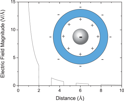
Figure 4: The magnitude of the approximate electric field (given by a set of Gauss surfaces, see inset) used to represent the fields in Figs. 2 and 3, and also used to calculate the energy contained in each layer (Eq. (4)).

Previously, we proposed a model for how the energy is depleted in a hydration layer as the effective radius of the pore, $R_{p}$, is reduced Zwolak09-1 . In this model, the energy change is proportional to the remaining surface area of a hydration layer within a pore. It takes into account both that the water-ion interaction energy of small water clusters is approximately linear in the number of waters Ignaczak99-1 ; Kistenmacher74-1 and that molecular dynamics simulations show a time-averaged water density with partial spherical shells when an ion is inside a pore of small enough radius (see Fig. 1 in Ref. Zwolak09-1 ). Contributions from, e.g., van der Waals interactions with the pore and changes in the water-water interaction, are small Yang07-1 ; Ignaczak99-1 . Thus, the energy of the remaining fraction $f_{i\nu}$ of the $i^{th}$ layer in the pore is taken as $U_{i\nu}=f_{i\nu}U_{i\nu}^{o}$. The fraction of the layer intact is $f_{i\nu}=S_{i\nu}/4\pi R_{i\nu}^{2}$ where $S_{i\nu}$ is the surface area (of the spherical layer) remaining where the water dipoles can fluctuate. The latter is given by

$$S_{i\nu}=2\Theta\left(R_{i\nu}-R_{p}\right)\int_{0}^{2\pi}d\phi\int_{0}^{\theta_{c\nu}}d\theta R_{i\nu}^{2}\sin\theta,$$ (5)

where $\Theta\left(x\right)$ is the step function and $\theta_{c\nu}=\sin^{-1}(R_{p}/R_{i\nu})$. When $R_{p}<R_{i\nu}$, the fraction of the surface left is

$$f_{i\nu}\left(R_{p}\right)=1-\sqrt{1-\left(\frac{R_{p}}{R_{i\nu}}\right)^{2}}.$$ (6)

The total internal energy change will then result from summing this fractional contribution over the layers to get

$$\Delta U_{\nu}(R_{p})=\sum_{i}(f_{i\nu}(R_{p})-1)U_{i\nu}^{o}.$$ (7)

We stress first that the effective radius $R_{p}$ is not necessarily the nominal radius defined by the pore atoms. Rather, it is the one that forces the hydration layer to be partially broken because it can not fit within the pore, and it could be smaller than the nominal pore radius by the presence of, e.g., a layer of tightly bound water molecules on the interior surface of the pore. Second, our model misses internal features of the hydration layers themselves. For instance, Ref. Song09-1 examines the first hydration layer structure in carbon nanotubes of different radii. These authors find a large increase in the energy barrier when the pore radius nears the inner hydration layer. They also seem to observe sub-steps in the water coordination number within the inner shell as the pore radius is reduced. Thus, although our model contains only a single “smoother” step, experiments could very well observe these internal sub-steps corresponding to the sudden loss of a single or few water molecules out of a given hydration layer.

Another basic assumption in our model is that the interaction energy of the water molecules in each layer is the same regardless of whether the ion is inside or outside of the pore. Figure 5 shows the distribution of the dipole orientation of water molecules both in bulk and inside pores of different radius . The average dipole orientation of the waters changes very little inside the pore, as do their fluctuations, thus supporting this assumption. In addition, the structure of the first two hydration layers (not shown) is essentially the same in and out of the smallest ($8\,\textrm{\AA}$) pore.

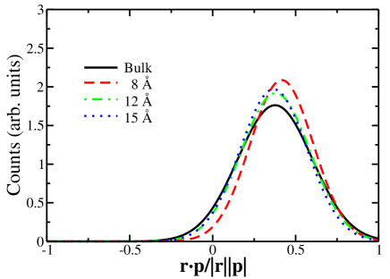
Figure 5: Distributions of the dipole orientations of water molecules within a cylindrical annulus $5\,\textrm{\AA}$ away from, i.e., in the second hydration layer of, a $\mathrm{Ca}^{2+}$ ion in bulk (black line) and inside pores of radius $8\,\textrm{\AA}$ (red dashed line), $12\,\textrm{\AA}$ (green dash-dotted line) and $15\,\textrm{\AA}$ (blue dotted line). The mean value is around $0.38$ (corresponding to the water dipole pointing 68 degrees away from the ion-water vector), except for the $8\,\textrm{\AA}$ pore, which increases to 0.42 (corresponding to the water dipole pointing 65 degrees away from the ion-water vector). This signifies a moderate tightening of the water dipole around the field of the ion as the pore size is reduced.

In order to make a connection with the ionic current (in Sec. IV below), we calculate the free energy change for species $\nu$ as

$$\Delta F_{\nu}=\Delta U_{\nu}-T\Delta S_{\nu},$$ (8)

which includes an entropic contribution from removing a single ion from solution and localizing it in the pore region. This entropic contribution is $\Delta S_{\nu}=k_{B}\ln\left(V_{p}n_{0}\right)$, where we have assumed an ideal ionic solution and $V_{p}$ is the volume of the pore and $n_{0}$ is the bulk salt concentration for all species $\nu$. The free energy change is plotted in Figs. 6 and 7 versus the effective pore radius and it is substantial when the latter becomes smaller than the outer hydration layer.

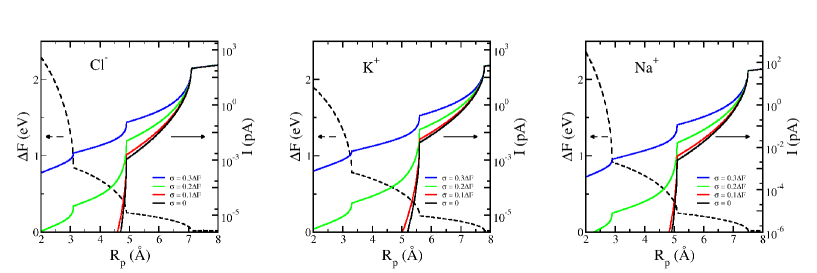
Figure 6: Free energy changes, $\Delta F_{\nu}$, and currents versus the effective pore radius for the monovalent ions and a field of $1\,\mathrm{mV/\textrm{\AA}}$. The black, dashed line indicates the free energy change. The remaining lines indicate the current with different standard deviations of the noise (see text for details). The currents are for $\sigma=p\Delta F$, with $p=0.3,\,0.2,\,0.1,\,0$ from top to bottom.

Figure 7: Free energy changes, $\Delta F_{\nu}$, and currents versus the effective pore radius for the divalent ions and a field of $1\,\mathrm{mV/\textrm{\AA}}$. The black, dashed line indicates the free energy change. The remaining lines indicate the current with different standard deviations of the noise (see text for details). The currents are for $\sigma=p\Delta F$, with $p=0.3,\,0.2,\,0.1,\,0$ from top to bottom.

IV Ionic Currents

We now want to relate these energy barriers to the ionic current through the pore . We do this by solving the Nernst-Planck equation in one dimension. Since this model consistently solves for both drift and diffusion contributions to ionic transport, and yields a compact analytical expression, we use it below with the energetic barriers found from the above model of dehydration. Even though this analytical model does not include some effects such as ion-ion interaction, we expect that it is qualitatively accurate as discussed along with its derivation.

The steady-state Nernst-Planck equation (see, e.g., Neumcke69-1 ; Eisenberg95-1 ; Hille01-1 ) for species $\nu$ in one dimension (assuming variability on the pore cross-section is not important) is

$$J_{\nu}=-q_{\nu}D_{\nu}\left[\frac{dn_{\nu}\left(z\right)}{dz}+\frac{q_{\nu}}{k_{B}T}n_{\nu}\left(z\right)\frac{d\Phi_{\nu}\left(z\right)}{dz}\right],$$ (9)

where $J_{\nu}$ is the charge flux for species $\nu$, $z\in\left(0,l\right)$ is the axial coordinate along the pore axis of length $l$, $n_{\nu}\left(z\right)$ is the ion density, $D_{\nu}$ is the diffusion coefficient (assumed to be position independent), and $\Phi_{\nu}\left(z\right)$ is the position-dependent potential (including both electrostatic and other interactions that change the energy within the pore). A full solution would require solving the density and potential within the reservoirs and pore simultaneously (see, e.g., Ref. Luchinsky09-1 ). However, we deal with high-resistance pores. Thus, we approximate the left ($L$) and right ($R$) reservoirs with constant concentrations $n_{L}$ and $n_{R}$, and the boundary conditions at the edge of the pore are $n_{\nu}\left(0\right)=n_{L}$ and $n_{\nu}\left(l\right)=n_{R}$. This is equivalent to assuming that as soon as an ion leaves or enters the pore, the ions in the immediate surroundings of the pore equilibrate rapidly to their prior distributions. Thus, multiplying by $\exp\left(q_{\nu}\Phi_{\nu}\left(z\right)/k_{B}T\right)$ to get

$$J_{\nu}e^{q_{\nu}\Phi_{\nu}\left(z\right)/k_{B}T}=-q_{\nu}D_{\nu}\frac{d}{dz}\left[n_{\nu}\left(z\right)e^{q_{\nu}\Phi_{\nu}\left(z\right)/k_{B}T}\right]$$ (10)

and integrating yields the flux for species $\nu$ as

$$J_{\nu}=-q_{\nu}D_{\nu}\frac{n_{R}e^{q_{\nu}\Phi_{\nu}\left(l\right)/k_{B}T}-n_{L}e^{q_{\nu}\Phi_{\nu}\left(0\right)/k_{B}T}}{\int_{0}^{l}dze^{q_{\nu}\Phi_{\nu}\left(z\right)/k_{B}T}}.$$ (11)

We make the further simplifying assumption that the electrostatic potential drops linearly over the pore - recognizing that in the presence of a significant potential barrier, e.g., due to the stripping of the water molecules from the hydration layers and in the absence of surface/fixed charges in the pore, the ionic density in the pore is small and thus the field is due to ionic charge layers on both sides of the pore. Results from many works that include ion-ion interactions indeed find a linear drop of the potential across the pore (see, e.g., Ref. Krems10-1 ). In this case, ions form a capacitor across the pore and every so often one ion translocates through the pore. The “healing” time for the loss of this ion is very short Krems10-1 and, thus, the field (potential drop) is not strongly affected . Also, we assume that the potential barrier due to changes in these other interactions is constant over the pore - this ignores a region near the pore entrance, but will not qualitatively change the solution. Therefore, the potential for species $\nu$ can be written as

$$\Phi_{\nu}\left(z\right)=z\frac{V}{l}+\frac{\Delta F_{\nu}}{q_{\nu}}$$ (12)

when $z\in\left(0,l\right)$. The boundaries are given by $\Phi_{z}\left(0\right)=0$ and $\Phi_{z}\left(l\right)=V$. Performing the remaining integral and for equal reservoir densities (our case), $n_{L}=n_{R}=n_{0}$, we get

$$J_{\nu}=-\frac{q_{\nu}^{2}n_{0}D_{\nu}V}{lk_{B}T}e^{-\Delta F_{\nu}/k_{B}T}.$$ (13)

Relating the diffusion coefficient to the mobility via the Einstein relation, $\mu_{\nu}=q_{\nu}D_{\nu}/k_{B}T$ , and putting in the constant electric field $E=V/l$, one obtains

$$J_{\nu}=-q_{\nu}n_{0}\mu_{\nu}Ee^{-\Delta F_{\nu}/k_{B}T}.$$ (14)

That is, the flux of an ionic species is proportional to the electric field and density, where the latter is suppressed by a Boltzmann factor Zwolak09-1 .

Now that we have an expression relating the energy barrier to the transport properties, we can calculate the current as a function of effective pore radius by multiplying Eq. (14) by the area of the pore to get

$$I_{\nu} =2\pi R_{p}^{2}J_{\nu}$$

$$\equiv I_{\nu 0}e^{-\Delta F_{\nu}/k_{B}T},$$ (15)

where we have defined a standard current $I_{\nu 0}=-q_{\nu}n_{0}2\pi R_{p}^{2}\mu_{\nu}E$ that would flow in the absence of an energy barrier. The current (15), with the mobilities and energies in Table 1, along with Eqs. (4)-(8), is plotted in Figs. 6 and 7 as a function of effective pore radius and for a field of $1\,\mathrm{mV/\textrm{\AA}}$ . The energetic barriers create sudden drops when the pore radii are congruent with a hydration layer radius. These correspond to the quantized steps in the conductance.

V Effect of noise

In a real experiment, there will also be fluctuations in the energetic barrier due to the fact that the hydration layers are not defined by their time-averaged value (i.e., they are not perfect spherical shells) and also due to fluctuations of the water structure and contents of the pore (both within a single experiment and also structural variations between experiments). Thus, we also examine the effect of these fluctuations and the current noise they induce. Thus, we calculate an averaged current for species $\nu$ as

$$\langle I_{\nu}\rangle=\langle I_{\nu 0}e^{-\Delta F_{\nu}/k_{B}T}\rangle.$$ (16)

We consider two specific models: Gaussian fluctuations of the free energy with a standard deviation proportional to the free energy barrier at a fixed pore radius and Gaussian fluctuations in the effective pore radius. The latter was also considered previously Zwolak09-1 where it was found that this type of noise smooths out the visibility of the drops in conductance (i.e., the peaks in the derivative $d\langle I_{\nu}\rangle/dR_{p}$ become smoother with increasing noise). However, it was also shown that this fluctuation induces a peak in the relative current noise that is much less sensitive to the strength of the fluctuations - thus giving an alternative method to detect the effect of the hydration layers. We develop a model for this relative noise here but do not perform the calculation of Eq. (16) for all the different species.

Fluctuating energy barrier - The first model we consider is an energy barrier that fluctuates according to a Gaussian distribution. We neglect fluctuations that make the barrier negative, so that the average current is

$$\langle I_{\nu}\rangle=\frac{I_{\nu 0}}{\mathcal{N}_{\sigma}}\int_{0}^{\infty}d\left(\Delta F\right)\,e^{-\Delta F/k_{B}T}e^{-(\Delta F-\Delta F_{\nu})^{2}/2\sigma^{2}},$$ (17)

where $\sigma$ is the standard deviation of the fluctuations and

$$\mathcal{N}_{\sigma}=\int_{0}^{\infty}d\left(\Delta F\right)e^{-(\Delta F-\Delta F_{\nu})^{2}/2\sigma^{2}}$$ (18)

is the normalization. The average current is thus

$$\langle I_{\nu}\rangle=I_{\nu 0}Ae^{-\left(\Delta F_{\nu}-\sigma^{2}/2k_{B}T\right)/k_{B}T},$$ (19)

where the factor $A$ is

$$A=\frac{\mathrm{erfc}\left[\left(-\Delta F_{\nu}+\sigma^{2}/k_{B}T\right)/\sqrt{2\sigma^{2}}\right]}{\mathrm{erfc}\left[-\Delta F_{\nu}/\sqrt{2\sigma^{2}}\right]}.$$ (20)

The value of $A$ for small $\sigma$ is very close to $1$. Thus, the effect of a fluctuating energy barrier with small fluctuations is simply to lower the energy barrier by an amount $\sigma^{2}/2k_{B}T$. For stronger fluctuations, the factor containing the complementary error function, $\mathrm{erfc}$, gives different limiting dependencies of the average current as the fluctuation strength $\sigma$ is increased. However, large fluctuations are well outside the realm of validity of the present model.

The relative noise in the current provides even more information. The relative noise is

$$\Delta I_{\mathrm{rel}}=\frac{\sqrt{\langle I^{2}\rangle-\langle I\rangle^{2}}}{\langle I\rangle}.$$ (21)

The expectation value of the square of the current is given by

$$\langle I_{\nu}^{2}\rangle =\frac{I_{\nu 0}}{\mathcal{N}_{\sigma}}\int_{0}^{\infty}d\left(\Delta F\right)\,e^{-\Delta F/k_{B}T}e^{-(\Delta F-\Delta F_{\nu})^{2}/2\sigma^{2}}$$

$$=BI_{\nu 0}^{2}e^{-\left(2\Delta F_{\nu}-2\sigma^{2}/k_{B}T\right)/k_{B}T}.$$ (22)

Where the normalization is as before and the factor $B$ is given by

$$B=\frac{\mathrm{erfc}\left[\left(-\Delta F_{\nu}+2\sigma^{2}/k_{B}T\right)/\sqrt{2\sigma^{2}}\right]}{\mathrm{erfc}\left[-\Delta F_{\nu}/\sqrt{2\sigma^{2}}\right]}.$$ (23)

Thus, the relative current noise induced by an energy barrier with fluctuations is

$$\Delta I_{rel}=\sqrt{e^{\sigma^{2}/\left(k_{B}T\right)^{2}}\frac{B}{A^{2}}-1}.$$ (24)

For small fluctuations, $A$ and $B$ depend very weakly on $\sigma$ and are both very close to $1$, giving a relative current noise

$$\Delta I_{rel}\approx\sigma/k_{B}T.$$ (25)

As expected, the relative noise increases with the strength of the fluctuations. For fluctuations proportional to the energy barrier, as shown in the Figs. 6 and 7, the fluctuations give rise to a monotonic increase in the relative noise. Overall, the effect of fluctuations in the energy barrier is to decrease the effective energy barrier and increase the current. This reduces the magnitude of the drops in the conductance but does not destroy their visibility. This would therefore help in observing quantized ionic conductance. It is worth noting, however, that this type of noise makes the step of the third hydration layer the most pronounced. This seems an unlikely situation in actual experiments and other types of noise need to be considered.

Fluctuating effective pore radius - In addition to the above noise, one expects that there would be fluctuations in the radii of the hydration layer/nanopore system. Previously, we demonstrated that this type of noise can smear the effect of the steps in the current Zwolak09-1 . As was seen, however, this noise also gives a peak in the relative noise in the current that is much less sensitive to the fluctuations than the average current. Here we develop a model of this behavior by calculating the relative noise assuming fluctuations across a single, perfect step in the free energy (see the inset of Fig. 8).

The average current due to species $\nu$ when averaged over fluctuations in the effective pore radius is

$$\langle I_{\nu}\rangle=\frac{1}{\mathcal{N}_{\xi}}\int_{0}^{\infty}dR\,I_{\nu 0}(R)e^{-\Delta F(R)/k_{B}T}e^{-(R-R_{p})^{2}/2\xi^{2}},$$ (26)

where $\xi$ is the standard deviation of the radial fluctuations, $\mathcal{N}_{\xi}$ is the normalization, and the explicit $R$ dependence has been included in both the barrier $\Delta F$ and the prefactor $I_{\nu 0}$. The dominant factor is the exponential of the free energy barrier and the quadratic dependence of $I_{\nu 0}$ on $R$ can be ignored. For small fluctuations, the lower limit of the integral can be extended to $-\infty$ and $\mathcal{N}_{\xi}\to\sqrt{2\pi\xi^{2}}$ to give

$$\langle I_{\nu}\rangle=\frac{I_{\nu 0}(R_{p})}{\sqrt{2\pi\xi^{2}}}\int_{-\infty}^{\infty}dR\,e^{-\Delta F(R)/k_{B}T}e^{-(R-R_{p})^{2}/2\xi^{2}}.$$ (27)

Previously, we performed the averaging according to Eq. (26) Zwolak09-1 , but here we instead use Eq. (27) with the approximate energy barrier $\Delta F\left(R\right)=\Delta F_{h}\Theta\left(R_{h}-R\right)$ of a single hydration layer of radius $R_{h}$ and take $\bar{I}_{\nu 0}$ to be the current in the absence of the barrier. The average current then becomes

$$\langle I_{\nu}\rangle=\bar{I}_{\nu 0}\left[e^{-\Delta F_{h}/k_{B}T}\left(1-C\right)+C\right],$$ (28)

where

$$C=\frac{1}{2}\mathrm{erfc}\left(\frac{R_{h}-R_{p}}{\sqrt{2}\xi}\right).$$ (29)

Similarly, for the square of the current one finds

$$\langle I_{\nu}^{2}\rangle=\bar{I}_{\nu 0}^{2}\left[e^{-2\Delta F_{h}/k_{B}T}\left(1-C\right)+C\right].$$ (30)

Although $\langle I_{\nu}\rangle$ and $\langle I_{\nu}^{2}\rangle$ are dependent on the strength of the fluctuations, $\xi$, the relative current noise has a universal behavior in the parameter $\tilde{R}=\left(R_{h}-R_{p}\right)/\sqrt{2}\xi$. That is, all features in the relative noise would be present regardless of the strength of the noise. However, the peak in the noise (see below) shifts to smaller values of $R_{p}$ as the noise strength is increased, which is qualitatively in agreement with the full averaging (Eq. (26)) performed in Ref. Zwolak09-1 .

The relative noise is

$$\Delta I_{\mathrm{rel}}=\frac{\sqrt{\left(1-e^{-\Delta F_{h}/k_{B}T}\right)^{2}C\left(1-C\right)}}{e^{-\Delta F_{h}/k_{B}T}\left(1-C\right)+C}.$$ (31)

For large or small $R_{p}$, the relative noise goes to zero, which can be seen from the properties of $\mathrm{erfc}$ that make $C\to 1$ and $C\to 0$ for large and small $R_{p}$, respectively. In between these limits, there would be nonzero relative noise, therefore indicating that the relative noise would have a maximum. The peak in the relative noise occurs for $R_{p}<R_{h}$. For a large energy barrier $\Delta F_{h}$, this peak occurs when $C$ is small. Thus, we can approximate the relative noise as

$$\Delta I_{\mathrm{rel}}\approx\frac{\sqrt{C}}{e^{-\Delta F_{h}/k_{B}T}+C}.$$ (32)

This gives a peak in the noise when $C=e^{-\Delta F_{h}/k_{B}T}$ with a value

$$\Delta I_{\mathrm{rel}}^{\star}\approx\frac{1}{2}e^{\Delta F_{h}/2k_{B}T}.$$ (33)

The peak is exponentially large in the energy barrier. However, the model with the electrostatic energy given by Eq. (7) does not have an ideal step in the free energy (see, e.g., Figs. 6 and 7). From previous work Zwolak09-1 , we can identify the peaks, $R_{p}^{\star}$, and use $\Delta F_{h}\approx\Delta F_{\nu}\left(R_{p}^{\star}\right)$. This is done in Fig. 8 for $\mathrm{Cl}^{-}$. The model agrees quantitatively with the full averaging performed in Ref. Zwolak09-1 . The only feature missing is the additional background noise away from the step due to the non-uniform energy barrier on both sides of the step.

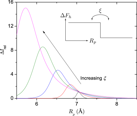
Figure 8: Relative current noise induced by structural fluctuations in the effective pore radius and/or hydration layer radius. The inset shows the approximate change in free energy $\Delta F_{h}$ as a function of effective pore radius in proximity to a hydration layer structure. The noise in the pore radius induces fluctuations between the high and low energy states. Here the third hydration layer radius of $\mathrm{Cl}^{-}$ is taken, $R_{h}=7.1\,\textrm{\AA}$. See the text for details on $\Delta F_{h}$. The fluctuation strength from right to left is $\xi=0.05,\,0.15,\,0.25,\,0.35,\,0.45\,\textrm{\AA}$.

Thus, from this “two-channel” model of noise we have found two generic features: (i) a peak develops in the relative current noise that is exponentially high with the hydration energy barrier, and (ii) it is present regardless of the noise strength, although its location moves to smaller values of the pore radius with increasing noise (likewise, the peak becomes wider). These features are in agreement with what is found from performing the full averaging from Eq. (26) using the surface area model of the energy barrier Zwolak09-1 . In the full model the fluctuations will eventually smooth out the peak in the relative current noise. The latter, however, is still much less sensitive than the average current drops, making the peak in the relative current noise versus $R_{p}$ a robust indicator of dehydration.

Barrier reduction - In addition to the above fluctuations, there are factors that reduce the energetic barrier, such as the presence of some surface charge and/or dielectric screening in the pore. In Eq. (4) we included a dielectric constant $\epsilon_{p}$ to represent a reduction in the hydration layer energy barrier from these sources. We expect, however, that the introduction of this constant overestimates the barrier reduction. It amounts to replacing the water molecules screening the ion with a material of lower dielectric constant but in the exact geometry of the water molecules. This is very unlikely since the pore screening comes from the fixed surface of the pore and thus in a different functional form. Nevertheless, it is instructive to see how the drops in the current are reduced by this effective lowering of the energy barrier. Figures 9 and 10 show the energy barrier and current for several values of this effective dielectric constant. We find that even for fairly large $\epsilon_{p}$ ($\sim 7$), the barriers are large enough to give a noticeable drop in the current.

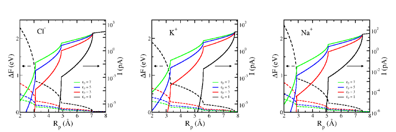
Figure 9: Free energy changes, $\Delta F$, and currents versus the effective pore radius for the monovalent ions and several values of $\epsilon_{p}$ ($\epsilon_{p}=7,\,5,\,3,\,1$ from bottom to top) and for a field of $1\,\mathrm{mV/\textrm{\AA}}$. The dashed lines indicate the free energy change. The solid lines indicate the current (see text for details). The currents are for $\epsilon_{p}=7,\,5,\,3,\,1$, from top to bottom.

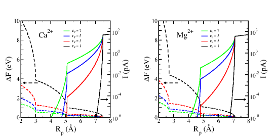
Figure 10: Free energy changes, $\Delta F$, and currents versus the effective pore radius for the divalent ions and several values of $\epsilon_{p}$ ($\epsilon_{p}=7,\,5,\,3,\,1$ from bottom to top) and for a field of $1\,\mathrm{mV/\textrm{\AA}}$.The dashed lines indicate the free energy change. The solid lines indicate the current (see text for details). The currents are for $\epsilon_{p}=7,\,5,\,3,\,1$, from top to bottom.

Bulk concentration - We also mention the effect of changing the concentration of ions in bulk. We have assumed that the hydration layers are well formed away from the pore. Large ionic concentration in bulk, however, would affect the formation of the hydration layers. For a completely disassociated 1:1 salt, the ion-ion distance goes as $\sim 9.4/n_{0}^{1/3}\,\textrm{\AA}$ where the bulk concentration, $n_{0}$, is given in mols/L. Thus, the inter-ion distance is $\sim 9.4\,\textrm{\AA}$ for a 1 M solution, which is almost large enough to house both the first and second hydration layers. However, concentrations lower than 1 M are preferable.

Some remarks - We have discussed many of the factors that will affect the detection of quantized ionic conductance. The most ideal experiment would be one with pores of well-controlled diameter and with smooth surfaces. Likewise, a small (or no) amount of surface charge and a low dielectric constant of the pore will make the effect more pronounced (and the ability to gate a pore, e.g., made of a nanotube, would help even more in understanding the energetics of transport). Not having these factors under control greatly affects the transport properties of the ions Chu2009-1 . Therefore, pores made of, for instance, semiconducting nanotubes may be ideal. Indeed, pores made of these materials have been recently demonstrated Liu2010-1 . However, rough surfaces that are present in pores made of, e.g., silicon nitride, should still allow for quantized conductance to be observed, so long as the variation of the effective radius of the pore is not too strong. The noise in the effective radius of the pore was investigated previously in Ref. Zwolak09-1 , where we found that only beyond variation in the radius of $0.2-0.3\,\textrm{\AA}$ will the effect be washed out. However, even beyond this variation magnitude, the relative current noise signifies the presence of steps in the energy barrier, thus giving a more robust indicator of the hydration layers’ effect on transport.

VI Conclusions

Ionic transport in nanopores is a fascinating subject with a long history and impact in many areas of science and technology. Recent work on developing aqueous-based nanotechnology and understanding biological ion channels requires a firm understanding of how water and ions behave in confined geometries and under non-equilibrium conditions due to applied fields. For example, the quest for ultra-fast, single-molecule DNA sequencing has yielded a number of proposals based on nanopores Zwolak08-1 . Among them, transverse electronic transport Zwolak05-1 ; Lagerqvist06-1 (whose theoretical basis includes the investigation of atomistic fluctuations Zwolak05-1 ; Lagerqvist06-1 ; Lagerqvist07-1 ; Lagerqvist07-2 and electronic noise in liquid environments Krems09-1 ) and ionic blockade Kasianowicz1996-1 ; Akeson1999-1 ; Deamer2000-1 ; Vercoutere2001-1 ; Deamer2002-1 ; Vercoutere2002-1 ; Vercoutere2003-1 ; Winters-Hilt2003-1 have yielded promising recent experiments (Refs. Tsutsui10-1 ; Chang10-1 and Clarke09-1 ; Stoddart09-1 , respectively). In all these cases, both water and ions are present and will have a significant impact on the signals and noise observed.

In this work, we have analyzed in detail the recent prediction of quantized ionic conductance Zwolak09-1 and examined how different aspects of the ion-nanopore system influence the detection of this phenomenon. Namely, we have shown that the ion type affects very little the radii at which the conduction should drop. High valency ions, however, should give even more pronounced drops in the current and thus may help in detecting this effect. Further, the presence of the hydration layers gives a peak in the relative noise at pore radii congruent with a layer radius. This relative noise is much less sensitive to fluctuations than the average current, and provides a promising approach to detect the effect of hydration.

Overall, quantized ionic conductance yields experimental predictions that will shed light on the contribution of dehydration to ion transport and we hope this work will motivate experiments in this direction.

- (1) B. Hille, Ion Channels of Excitable Membranes (Sinauer Associates, Sunderland, 2001)
- (2) F. M. Ashcroft, Ion channels and disease (Academic Press, San Diego, 2000)
- (3) M. Zwolak and M. Di Ventra, Rev. Mod. Phys. 80, 141 (2008)
- (4) M. Zwolak and M. Di Ventra, Nano Lett. 5, 421 (2005)
- (5) J. Lagerqvist, M. Zwolak, and M. DiVentra, Nano Lett. 6, 779 (2006)
- (6) J. Lagerqvist, M. Zwolak, and M. Di Ventra, Biophys. J. 93, 2384 (2007)
- (7) J. Lagerqvist, M. Zwolak, and M. Di Ventra, Phys. Rev. E 76, 013901 (2007)
- (8) M. Krems, M. Zwolak, Y. V. Pershin, and M. Di Ventra, Biophys. J. 97, 1990 (2009)
- (9) J. B. Heng, A. Aksimentiev, C. Ho, V. Dimitrov, T. W. Sorsch, J. F. Miner, W. M. Mansfield, K. Schulten, and G. Timp, Bell Labs Technical Journal 10, 5 (2005)
- (10) M. E. Gracheva, A. Xiong, A. Aksimentiev, K. Schulten, G. Timp, and J.-P. Leburton, Nanotechnology 17, 622 (2006)
- (11) M. E. Gracheva, A. Aksimentiev, and J.-P. Leburton, Nanotechnology 17, 3160 (2006)
- (12) J. J. Kasianowicz, E. Brandin, D. Branton, and D. W. Deamer, Proc. Natl. Acad. Sci. U. S. A. 93, 13770 (1996)
- (13) M. Akeson, D. Branton, J. J. Kasianowicz, E. Brandin, and D. W. Deamer, Biophys. J. 77, 3227 (1999)
- (14) D. W. Deamer and M. Akeson, Trends Biotechnol. 18, 147 (2000)
- (15) W. Vercoutere, S. Winters-Hilt, H. Olsen, D. Deamer, D. Haussler, and M. Akeson, Nat. Biotechnol. 19, 248 (2001)
- (16) D. W. Deamer and D. Branton, Acc. Chem. Res. 35, 817 (2002)
- (17) W. Vercoutere and M. Akeson, Curr. Opin. Chem. Biol. 6, 816 (2002)
- (18) W. A. Vercoutere, S. Winters-Hilt, V. S. DeGuzman, D. Deamer, S. E. Ridino, J. T. Rodgers, H. E. Olsen, A. Marziali, and M. Akeson, Nucleic Acids Res. 31, 1311 (2003)
- (19) S. Winters-Hilt, W. Vercoutere, V. S. DeGuzman, D. Deamer, M. Akeson, and D. Haussler, Biophys. J. 84, 967 (2003)
- (20) M. Tsutsui, M. Taniguchi, K. Yokota, and T. Kawai, Nat Nano 5, 286 (2010)
- (21) S. Chang, S. Huang, J. He, F. Liang, P. Zhang, S. Li, X. Chen, O. Sankey, and S. Lindsay, Nano Lett. 10, 1070 (2010)
- (22) J. Clarke, H.-C. Wu, L. Jayasinghe, A. Patel, S. Reid, and H. Bayley, Nat Nano 4, 265 (2009)
- (23) D. Stoddart, A. J. Heron, E. Mikhailova, G. Maglia, and H. Bayley, Proc. Natl. Acad. Sci. U. S. A. 106, 7702 (2009)
- (24) D. A. Doyle, J. a. M. Cabral, R. A. Pfuetzner, A. Kuo, J. M. Gulbis, S. L. Cohen, B. T. Chait, and R. MacKinnon, Science 280, 69 (1998)
- (25) S.-H. Chung, O. S. Anderson, and V. V. Krishnamurthy, Biological Membrane Ion Channels: Dynamics, Structure, and Applications (Springer, New York, 2007)
- (26) M. Thomas, D. Jayatilaka, and B. Corry, Biophys. J. 93, 2635 (2007)
- (27) S. Varma and S. B. Rempe, Biophys. J. 93, 1093 (2007)
- (28) P. W. Fowler, K. Tai, and M. S. P. Sansom, Biophys. J. 95, 5062 (2008)
- (29) T. Dudev and C. Lim, J. Am. Chem. Soc. 131, 8092 (2009)
- (30) D. L. Bostick and C. L. Brooks, Proc. Natl. Acad. Sci. U. S. A. 104, 9260 (2007)
- (31) H. Yu, S. Y. Noskov, and B. Roux, J. Phys. Chem. B 113, 8725 (2009)
- (32) D. L. Bostick and C. L. Brooks 96, 4470 (2009)
- (33) J. Li, D. Stein, C. McMullan, D. Branton, M. J. Aziz, and J. A. Golovchenko, Nature (London, U. K.) 412, 166 (2001)
- (34) S. A. Miller, V. Y. Young, and C. R. Martin, J. Am. Chem. Soc. 123, 12335 (2001)
- (35) A. J. Storm, J. H. Chen, X. S. Ling, H. Zandbergen, and C. Dekker, Nat. Mater. 2, 537 (2003)
- (36) J. K. Holt, A. Noy, T. Huser, D. Eaglesham, and O. Bakajin, Nano Lett. 4, 2245 (2004)
- (37) Z. Siwy, E. Heins, C. C. Harrell, P. Kohli, and C. R. Martin, J. Am. Chem. Soc. 126, 10850 (2004)
- (38) C. C. Harrell, P. Kohli, Z. Siwy, and C. R. Martin, J. Am. Chem. Soc. 126, 15646 (2004)
- (39) J. K. Holt, H. G. Park, Y. Wang, M. Stadermann, A. B. Artyukhin, C. P. Grigoropoulos, A. Noy, and O. Bakajin, Science 312, 1034 (2006)
- (40) C. Dekker, Nat Nano 2, 209 (2007)
- (41) M. Zwolak, J. Lagerqvist, and M. Di Ventra, Phys. Rev. Lett. 103, 128102 (2009)
- (42) M. Di Ventra, Electrical Transport in Nanoscale Systems (Cambridge University Press, Cambridge, 2008)
- (43) A. Parsegian, Nature 221, 844 (1969)
- (44) V. A. Parsegian, Ann. N. Y. Acad. Sci. 264, 161 (1975)
- (45) Y. Marcus, J. Chem. Soc., Faraday Trans. 87, 2995 (1991)
- (46) D. G. Levitt, Biophys. J. 22, 209 (1978)
- (47) P. C. Jordan, Biophys. Chem. 13, 203 (1981)
- (48) P. C. Jordan, Biophys. J. 39, 157 (1982)
- (49) B. Roux, T. Allen, S. Bernéche, and W. Im, Q. Rev. Biophys. 37, 15 (2004)
- (50) S. Teber, J. Stat. Mech. ,, P07001 (2005)
- (51) J. Zhang, A. Kamenev, and B. I. Shklovskii, Phys. Rev. Lett. 95, 148101 (2005)
- (52) A. Kamenev, J. Zhang, A. Larkin, and B. Shklovskii, Physica A 359, 129 (2006)
- (53) A. Finkelstein and O. S. Andersen, J. Membr. Biol. 59, 155 (1981)
- (54) J. H. Morais-Cabral, Y. Zhou, and R. MacKinnon, Nature 414, 37 (2001)
- (55) J. D. Jackson, Classical Electrodynamics, 3rd ed. (Wiley, 1998)
- (56) A. H. Narten, J. Chem. Phys. 56, 5681 (1972)
- (57) J. C. Phillips, R. Braun, W. Wang, J. Gumbart, E. Tajkhorshid, E. Villa, C. Chipot, R. D. Skeel, L. Kalé, and K. Schulten, J. Comput. Chem. 26, 1781 (2005)
- (58) H. Ohtaki and T. Radnai, Chem. Rev. 93, 1157 (1993)
- (59) L. Yang and S. Garde, J. Chem. Phys. 126, 084706 (2007)
- (60) A. Ignaczak, J. A. N. F. Gomes, and M. N. D. S. Cordeiro, Electrochim. Acta 45, 659 (1999)
- (61) H. Kistenmacher, H. Popkie, and E. Clementi, J. Chem. Phys. 61, 799 (1974)
- (62) C. Song and B. Corry, J. Phys. Chem. B 113, 7642 (2009)
- (63) B. Neumcke and P. Läuger, Biophys. J. 9, 1160 (1969)
- (64) R. S. Eisenberg, M. M. Klosek, and Z. Schuss, J. Chem. Phys. 102, 1767 (1995)
- (65) D. G. Luchinsky, R. Tindjong, I. Kaufman, P. V. E. McClintock, and R. S. Eisenberg, Phys. Rev. E 80, 021925 (2009)
- (66) M. Krems, Y. V. Pershin, and M. Di Ventra, Nano Lett. 10, 2674 (2010)
- (67) E. R. Cruz-Chu, A. Aksimentiev, and K. Schulten, J. Phys. Chem. C 113, 1850 (2009)
- (68) H. Liu, J. He, J. Tang, H. Liu, P. Pang, D. Cao, P. Krstic, S. Joseph, S. Lindsay, and C. Nuckolls, Science 327, 64 (2010)
- (69) A. A. Rashin and B. Honig, J. Phys. Chem. 89, 5588 (1985)
- (70) B. Roux, H. A. Yu, and M. Karplus, J. Phys. Chem. 94, 4683 (1990)