q-Analogue of Shock Soliton Solution

Abstract

By using Jackson’s q-exponential function we introduce the generating function, the recursive formulas and the second order q-differential equation for the q-Hermite polynomials. This allows us to solve the q-heat equation in terms of q-Kampe de Feriet polynomials with arbitrary N moving zeroes, and to find operator solution for the Initial Value Problem for the q-heat equation. By the q-analog of the Cole-Hopf transformation we construct the q-Burgers type nonlinear heat equation with quadratic dispersion and the cubic nonlinearity. In $q\rightarrow 1$ limit it reduces to the standard Burgers equation. Exact solutions for the q-Burgers equation in the form of moving poles, singular and regular q-shock soliton solutions are found.

1 Introduction

It is well known that the Burgers’ equation in one dimension could be linearized by the Cole-Hopf transformation in terms of the linear heat equation. It allows one to solve the initial value problem for the Burgers equation and to get exact solutions in the form of shock solitons and describe their scattering. In the present paper we study the q-differential Burgers type equation with quadratic dispersion and the cubic nonlinearity, and find its linearization in terms of the q-heat equation. In terms of the Jackson’s q-exponential function we introduce the q-Hermite and q-Kampe-de Feriet polynomials, representing moving poles solution for the q-Burgers equation. Then we derive the operator solution of the initial value problem for the q-Burgers equation in terms of the IVP for the q-heat equation. We find solutions of our q-Burgers type equation in the form of singular and regular q-shock solitons. It turns out that static q-shock soliton solution shows remarkable self-similarity property in space coordinate $x$.

2 q-Exponential Function

The q-number corresponding to the ordinary number $n$ is defined as, [1],

$$[n]_{q}=\frac{q^{n}-1}{q-1},$$ (1)

where $q$ is a parameter, so that $n$ is the limit of $[n]_{q}$ as $q\rightarrow 1$. A few examples of q-numbers are given here: $[0]_{q}=0$, $[1]_{q}=1$, $[2]_{q}=1+q$, $[3]_{q}=1+q+q^{2}$. In terms of these q-numbers, the Jackson q-exponential function is defined as

$$e_{q}(x)=\sum^{\infty}_{n=0}\frac{x^{n}}{[n]_{q}!}.$$ (2)

For $q>1$ it is entire function of $x$ and when $q\rightarrow 1$ it reduces to the standard exponential function $e^{x}$. The q-exponential function can also be expressed in terms of infinite product

$$e_{q}(x)=\prod^{\infty}_{n=0}\frac{1}{\left(1-(1-q)q^{n}x\right)}=\frac{1}{\left(1-(1-q)x\right)^{\infty}_{q}},$$ (3)

when $q<1$ and

$$e_{q}(x)=\prod^{\infty}_{n=0}{\left(1+(1-\frac{1}{q})\frac{1}{q^{n}}x\right)}={\left(1+(1-\frac{1}{q})x\right)^{\infty}_{1/q}},$$ (4)

when $q>1$. Thus, the q-exponential function for $q<1$ has infinite set of poles at

$$x_{n}=\frac{1}{q^{n}(1-q)},\,\,\,\,\,\,\,n=0,1,..$$ (5)

and for $q>1$ the infinite set of zeros at

$$x_{n}=-\frac{q^{n+1}}{(q-1)},\,\,\,\,\,\,\,n=0,1,..$$ (6)

The q-derivative is defined as

$$D^{x}_{q}f(x)=\frac{f(qx)-f(x)}{(q-1)x},$$ (7)

and when $q\rightarrow 1$ it reduces to the standard derivative $D^{x}_{q}f(x)\rightarrow f^{\prime}(x)$. Using the definition of the $q$-derivative one can easily see that

$$D^{x}_{q}(ax^{n})=a[n]_{q}x^{n-1},$$ (8)

$$D^{x}_{q}e_{q}(ax)=ae_{q}(ax).$$ (9)

3 q-Hermite Polynomials

We define the q-Hermite polynomials according to the generating function

$$e_{q}(-t^{2})e_{q}([2]_{q}tx)=\sum^{\infty}_{n=0}H_{n}(x;q)\frac{t^{n}}{[n]_{q}!}.$$ (10)

From this generating function we have the special values

$$H_{2n}(0;q)=(-1)^{n}\frac{[2n]_{q}!}{[n]_{q}!},$$ (11)

$$H_{2n+1}(0;q)=0,$$ (12)

where $[n]_{q}!=[1]_{q}[2]_{q}...[n]_{q}$, and the parity relation

$$H_{n}(-x;q)=(-1)^{n}H_{n}(x;q).$$ (13)

By q-differentiating the generating function (10) according to $x$ and $t$ we have the recurrence relations correspondingly

$$D_{x}H_{n}(x;q)=[2]_{q}[n]_{q}H_{n-1}(x;q),$$ (14)

$$H_{n+1}(x;q)=[2]_{q}\,xH_{n}(x;q)-[n]_{q}\,H_{n-1}(qx;q)\\ -[n]_{q}\,q^{\frac{n+1}{2}}H_{n-1}(\sqrt{q}x;q).$$

Using operator

$$M_{q}=q^{x\frac{d}{dx}},$$ (15)

so that

$$M_{q}f(x)=f(qx),$$ (16)

relation (3) can be rewritten as

$$H_{n+1}(x;q)=[2]_{q}\,xH_{n}(x;q)\\ -[n]_{q}(M_{q}+q^{\frac{n+1}{2}}M_{\sqrt{q}})H_{n-1}(x;q).$$

Substituting (14) to (3) we get

$$H_{n+1}(x;q)=\left([2]_{q}\,x-\frac{M_{q}+q^{\frac{n+1}{2}}M_{\sqrt{q}}}{[2]_{q}}D_{x}\right)H_{n}(x;q)$$ (17)

By the recursion, starting from $n=0$ and $H_{0}(x)=1$ we have next representation for the q-Hermite polynomials

$$H_{n}(x;q)=\prod^{n}_{k=1}\left([2]_{q}\,x-\frac{M_{q}+q^{\frac{k}{2}}M_{\sqrt{q}}}{[2]_{q}}D_{x}\right)\cdot 1$$ (18)

We notice that the generating function and the form of our q-Hermite polynomials are different from the known ones in the literature, [2], [4], [3], [5].
In the above expression the operator

$$M_{q}+q^{\frac{n}{2}}M_{\sqrt{q}}=2q^{\frac{n}{4}}q^{\frac{3}{4}x\frac{d}{dx}}\cosh[(\ln q^{\frac{1}{4}})(x\frac{d}{dx}-n)]$$ (19)

is expressible in terms of the q-spherical means as

$$\cosh[(\ln q)x\frac{d}{dx}]f(x)=\frac{1}{2}(f(qx)+f(\frac{1}{q}x)).$$ (20)

Using definition, [1],

$$(x-a)^{n}_{q}=(x-a)(x-qa)\cdot\cdot\cdot(x-q^{n-1}a),\,\,n=1,2,..$$

which now we apply for operators, we should distinguish the direction of multiplication. We consider two cases

$$(x-a)^{n}_{q\,<}=(x-a)(x-qa)\cdot\cdot\cdot(x-q^{n-1}a),$$ (21)

and

$$(x-a)^{n}_{q\,>}=(x-q^{n-1}a)\cdot\cdot\cdot(x-qa)(x-a).$$ (22)

Then, we can rewrite (18) shortly as

$$H_{n}(x;q)=\left(([2]_{q}\,x-\frac{M_{q}\,D_{x}}{[2]_{q}})-q^{\frac{1}{2}}\frac{M_{\sqrt{q}}\,D_{x}}{[2]_{q}}\right)^{n}_{\sqrt{q}\,>}\cdot 1$$

First few polynomials are

$$H_{0}(x;q)=1,$$

$$H_{1}(x;q)=[2]_{q}\,x,$$

$$H_{2}(x;q)=[2]^{2}_{q}\,x^{2}-[2]_{q},$$

$$H_{3}(x;q)=[2]^{3}_{q}\,x^{3}-[2]^{2}_{q}[3]_{q}\,x,$$

$$H_{4}(x;q)=[2]^{4}_{q}\,x^{4}-[2]^{2}_{q}[3]_{q}[4]_{q}\,x^{2}+[2]_{q}[3]_{q}[2]_{q^{2}}.$$

When $q\rightarrow 1$ these polynomials reduce to the standard Hermite polynomials.

3.1 q-Differential Equation

Applying $D_{x}$ to both sides of (17) and using recurrence formula (14) we get q-differential equation for q-Hermite polynomials

$$\frac{1}{[2]_{q}}D_{x}(M_{q}+q^{\frac{n+1}{2}}M_{\sqrt{q}})D_{x}H_{n}(x;q)-[2]_{q}qxD_{x}H_{n}(x;q)+[2]_{q}[n]_{q}qH_{n}(x;q)=0.$$

3.2 Operator Representation

Proposition 1

We have next identity

$$e_{q}\left(-\frac{1}{[2]_{q}}D^{2}_{x}\right)e_{q}([2]_{q}xt)=e_{q}(-t^{2})e_{q}([2]_{q}xt).$$ (23)

Proof 1

By q- differentiating the q-exponential function in $x$

$$D^{n}_{x}e_{q}([2]_{q}xt)=([2]t)^{n}e_{q}([2]_{q}xt),$$ (24)

and combining then to the sum

$$\sum_{n=0}^{\infty}\frac{a^{n}}{[n]_{q}!}D^{2n}_{x}e_{q}([2]_{q}xt)=\sum_{n=0}^{\infty}\frac{[2]_{q}^{n}a^{n}t^{2n}}{[n]_{q}!}\,\,e_{q}([2]_{q}xt),$$ (25)

we have relation

$$e_{q}(aD^{2}_{x})e_{q}([2]_{q}xt)=e_{q}([2]_{q}at^{2})e_{q}([2]_{q}xt).$$ (26)

By choosing $a=-1/[2]_{q}$ we get

$$e_{q}\left(-\frac{1}{[2]_{q}}D^{2}_{x}\right)e_{q}([2]_{q}xt)=e_{q}(-t^{2})e_{q}([2]_{q}xt).$$ (27)

Proposition 2

The next identity is valid

$$H_{n}(x;q)=[2]^{n}e_{q}\left(-\frac{1}{[2]_{q}}D^{2}_{x}\right)x^{n}.$$ (28)

Proof 2

The right hand side of (23) is the generating function for q-Hermite polynomials. Hence expanding both sides in $t$ we get the result.

Proposition 3

$$e_{q}\left(-\frac{D^{2}_{x}}{[2]_{q}}\right)x^{n+1}=\\ \frac{1}{[2]_{q}}\left([2]_{q}\,x-\frac{(M_{q}+q^{\frac{n+1}{2}}M_{\sqrt{q}})D_{x}}{[2]_{q}}\right)e_{q}\left(-\frac{D^{2}_{x}}{[2]_{q}}\right)x^{n}.$$

Proof 3

we use (28) and relation (17) .

Corrollary 1

If function $f(x)$ is analytic and expandable to power series $f(x)=\sum^{\infty}_{n=0}a_{n}x^{n}$ then we have next q-Hermite series

$$e_{q}\left(-\frac{1}{[2]_{q}}D^{2}_{x}\right)f(x)=\sum^{\infty}_{n=0}a_{n}\frac{H_{n}(x;q)}{[2]_{q}^{n}}.$$ (29)

4 q- Kampe-de Feriet Polynomials

We define q-Kampe-de Feriet polynomials as

$$H_{n}(x,t;q)=(-\nu t)^{\frac{n}{2}}H_{n}\left(\frac{x}{[2]_{q}\sqrt{-\nu t}}\right),$$ (30)

and from (17) we have the next recursion formula

$$H_{n+1}(x,t;q)=\left(x+(M_{q}+q^{\frac{n+1}{2}}M_{\sqrt{q}})\nu tD_{x}\right)H_{n}(x,t;q).$$

By recursion it gives

$$H_{n}(x,t;q)=\prod^{n}_{k=1}\left(x+(M_{q}+q^{\frac{k}{2}}M_{\sqrt{q}})\nu tD_{x}\right)\cdot 1$$ (31)

or by notation (22)

$$H_{n}(x,t;q)=\left((x+M_{q}\,\nu t\,D_{x})+q^{\frac{1}{2}}M_{\sqrt{q}}\,\nu tD_{x}\right)^{n}_{\sqrt{q}\,>}\cdot 1$$

First few polynomials are

$$H_{0}(x,t;q)=1,$$

$$H_{1}(x,t;q)=x,$$

$$H_{2}(x,t;q)=x^{2}+[2]_{q}\,\nu t,$$

$$H_{3}(x,t;q)=x^{3}+[2]_{q}[3]_{q}\,\nu t\,x,$$

$$H_{4}(x,t;q)=x^{4}+[3]_{q}[4]_{q}\,\nu t\,x^{2}+[2]_{q}[3]_{q}[2]_{q^{2}}\nu^{2}t^{2}.$$

5 q-Heat Equation

We consider the q-heat equation

$$(D_{t}-\nu D^{2}_{x})\phi(x,t)=0.$$ (32)

Solution of this equation expanded in terms of parameter $k$

$$\phi(x,t)=e_{q}(\nu k^{2}t)e_{q}(kx)=\sum^{\infty}_{n=0}\frac{k^{n}}{[n]!}H_{n}(x,t;q),$$ (33)

gives the set of q-Kampe-de Feriet polynomial solutions for the equation. Then we find time evolution of zeroes for these solutions in terms of zeroes $z_{k}(n,q)$ of q-Hermite polynomials,

$$H_{n}(z_{k}(n,q),q)=0,$$ (34)

so that

$$x_{k}(t)=[2]z_{k}(n,q)\sqrt{-\nu t}.$$ (35)

For n=2 we have two zeros determined by q-numbers,

$$x_{1}(t)={\sqrt{[2]_{q}}}\sqrt{-\nu t}\\ ,$$ (36)

$$x_{2}(t)=-{\sqrt{[2]_{q}}}\sqrt{-\nu t}\\ ,$$ (37)

and moving in opposite directions according to (35). For n=3 we have zeros determined by q-numbers,

$$x_{1}(t) = -\sqrt{{[3]_{q}!}}\sqrt{-\nu t},$$ (38)

$$x_{2}(t) = 0,$$ (39)

$$x_{3}(t) = \sqrt{{[3]_{q}!}}\sqrt{-\nu t},$$ (40)

two of which are moving in opposite direction according to (35) and one is in the rest.

6 Evolution Operator

Following similar calculations as in Proposition I we have next relation

$$e_{q}\left(\nu tD^{2}_{x}\right)e_{q}(kx)=e_{q}(\nu tk^{2})e_{q}(kx).$$ (41)

The right hand side of this expression is the plane wave type solution of the q-heat equation

$$(D_{t}-\nu D^{2}_{x})\phi(x,t)=0.$$ (42)

Expanding both sides in power series in $k$ we get q-Kampe de Ferie polynomial solutions of this equation

$$H_{n}(x,t;q)=e_{q}\left(\nu tD^{2}_{x}\right)x^{n}.$$ (43)

Consider an arbitrary analytic function $f(x)=\sum^{\infty}_{n=0}a_{n}x^{n}$, then function

$$f(x,t)=e_{q}\left(\nu tD^{2}_{x}\right)f(x) = \sum^{\infty}_{n=0}a_{n}e_{q}\left(\nu tD^{2}_{x}\right)x^{n}$$ (44)

$$= \sum^{\infty}_{n=0}a_{n}H_{n}(x,t;q),$$ (45)

is a time dependent solution of the q-heat equation (42).

According to this we have the evolution operator for the q-heat equation as

$$U(t)=e_{q}\left(\nu tD^{2}_{x}\right).$$ (46)

It allows us to solve the initial value problem

$$(D_{t}-\nu D^{2}_{x})\phi(x,t) = 0,$$ (47)

$$\phi(x,0^{+}) = f(x),$$ (48)

in the form

$$\phi(x,t)=e_{q}\left(\nu tD^{2}_{x}\right)\phi(x,0^{+})=e_{q}\left(\nu tD^{2}_{x}\right)f(x).$$ (49)

7 q-Burgers’ Type Equation

Let us consider the q-Cole-Hopf transformation

$$u(x,t)=-2\nu\frac{D_{x}\phi(x,t)}{\phi(x,t)},$$ (50)

then $u(x,t)$ satisfies the q-Burgers’ type Equation with quadratic dispersion and cubic nonlinearity

$$\begin{array}[]{l}D_{t}u(x,t)-D^{2}_{x}u(x,t)=\frac{1}{2}\left[(u(x,qt)-u(x,t)M^{x}_{q})D_{x}u(x,t)\right]-\\ \\ \frac{1}{2}\left[D_{x}\left(u(qx,t)u(x,t)\right)\right]+\frac{1}{4}\left[u(q^{2}x,t)-u(x,qt)\right]u(qx,t)u(x,t).\end{array}$$

When $q\rightarrow 1$ it reduces to the standars Burgers’ Equation.

7.1 I.V.P. for q-Burgers’ Type Equation

Substituting the operator solution (49) to (50) we find operator solution for the q-Burgers type equation in the form

$$u(x,t)=-2\nu\frac{e_{q}\left(\nu tD^{2}_{x}\right)D_{x}f(x)}{e_{q}\left(\nu tD^{2}_{x}\right)f(x)}.$$ (51)

This solution corresponds to the initial function

$$u(x,0^{+})=-2\nu\frac{D_{x}f(x)}{f(x)}.$$ (52)

Thus, for arbitrary initial value problem for the q-Burgers equation with $u(x,0^{+})=F(x)$ we need to solve the initial value problem for the q-heat equation with initial function $f(x)$ satisfying the first order q-differential equation

$$(D_{x}+\frac{1}{2\nu}F(x))f(x)=0.$$ (53)

8 q-Shock soliton solution

As a solution of q-heat equation we choose first

$$\phi(x,t)=e_{q}\left(k^{2}t\right)e_{q}\left(kx\right),$$ (54)

then we find solution of the q-Burgers equation as a constant

$$u(x,t)=-2\nu k.$$ (55)

If we choose

$$\phi(x,t)=e_{q}\left(k_{1}^{2}t\right)e_{q}\left(k_{1}x\right)+e_{q}\left(k_{2}^{2}t\right)e_{q}\left(k_{2}x\right),$$ (56)

then we have the q-Shock soliton solution

$$u(x,t)=-2\nu\frac{k_{1}e_{q}\left(k_{1}^{2}t\right)e_{q}\left(k_{1}x\right)+k_{2}e_{q}\left(k_{2}^{2}t\right)e_{q}\left(k_{2}x\right)}{e_{q}\left(k_{1}^{2}t\right)e_{q}\left(k_{1}x\right)+e_{q}\left(k_{2}^{2}t\right)e_{q}\left(k_{2}x\right)}.$$ (57)

Due to zeroes of the q-exponential function this expression admits singularities for some values of parameters $k_{1}$ and $k_{2}$. In Fig.1 we plot the singular q-shock soliton for $k_{1}=1$ and $k_{2}=10$ at time $t=0$.

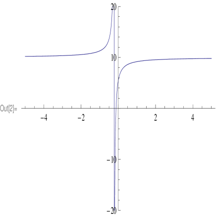
Figure 1: Singular q-Shock Soliton

However for some specific values of the parameters we found the regular q-shock soliton solution. We introduce the q-hyperbolic function

$$\cosh_{q}(x)=\frac{e_{q}(x)+e_{q}(-x)}{2},$$ (58)

or

$$\cosh_{q}(x)=\frac{1}{2}\left(e_{q}(x)+\frac{1}{e_{\frac{1}{q}}(x)}\right),$$ (59)

then by using infinite product representation for q-exponential function we have

$$\cosh_{q}(x)=\frac{1}{2}\left({\left(1+(1-\frac{1}{q})x\right)^{\infty}_{1/q}}+{\left(1-(1-\frac{1}{q})x\right)^{\infty}_{q}}\right).$$

From (5),(6) we find that zeroes of the first product are located on negative axis $x$, while for the second product on the positive axis $x$. Therefore the function has no zeros for real $x$ and $\cosh_{q}(0)=1$.

If $k_{1}=1$, and $k_{2}=-1$, the time dependent factors in nominator and the denominator of (57) cancel each other and we have the stationary shock soliton

$$u(x,t)=-2\nu\frac{e_{q}(x)-e_{q}(-x)}{e_{q}(x)+e_{q}(-x)}\equiv-2\nu\tanh_{q}(x).$$ (60)

Due to above consideration this function has no singularity on real axis and we have regular q-shock soliton.

In Fig.2, Fig.3 and Fig.4 we plot the regular q-shock soliton for $k_{1}=1$ and $k_{2}=-1$ at different ranges of $x$. It is remarkable fact that the structure of our shock soliton shows self-similarity property in space coordinate $x$. Indeed at the ranges of parameter $x=50,\,5000,\,500000$ the structure of shock looks almost the same.

Figure 2: Regular q-Shock Soliton For $k_{1}=1$, $k_{2}=-1$, at range (-50, 50)

Figure 3: The regular q-shock soliton for $k_{1}=1$, $k_{2}=-1$ at range (-5000, 5000)

Figure 4: The regular q-shock soliton for $k_{1}=1$, $k_{2}=-1$ at range (-500000, 500000)

For the set of arbitrary numbers $k_{1},...,k_{N}$

$$\phi(x,t)=\sum^{N}_{n=1}e_{q}\left(k_{n}^{2}t\right)e_{q}\left(k_{n}x\right),$$ (61)

we have multi-shock solution in the form

$$u(x,t)=-2\nu\frac{\sum^{N}_{n=1}k_{n}e_{q}\left(k_{n}^{2}t\right)e_{q}\left(k_{n}x\right)}{\sum^{N}_{n=1}e_{q}\left(k_{n}^{2}t\right)e_{q}\left(k_{n}x\right)}.$$ (62)

In general this solution admits several singularities. To have regular multi-shock solution we can consider the even number of terms $N=2k$ with opposite wave numbers. When $N=4$ and $k_{1}=1$, $k_{2}=-1$,$k_{3}=10$,$k_{4}=-10$ we have q-multi-shock soliton solution,

$$u(x,t)=-2\nu\frac{e_{q}(t)\sinh_{q}(x)+10e_{q}(100t)\sinh_{q}(10x)}{e_{q}(t)\cosh_{q}(x)+e_{q}(100t)\cosh_{q}(10x)}.$$ (63)

In Fig. 5 we plot $N=4$ case with values of the wave numbers $k_{1}=1$, $k_{2}=-1$,$k_{3}=10$,$k_{4}=-10$ at $t=0$. To have regular solution for any time $t$ and given base $q$, we should choose proper numbers $k_{i}$ which are not in the form of power of $q$. This question is under the study now.

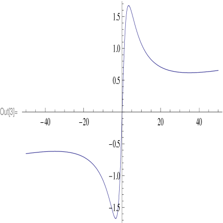
Figure 5: q-shock regular

References

- [1] V. Kac and P. Cheung, Quantum Calculus, Springer, New York, 2002.
- [2] H. Exton, q-Hypergeometric Functions and Applications, John Wiley and Sons, 1983.
- [3] P. Rajkovic and S. Marinkovic, On Q-analogies of generalized Hermite’s polynomials, Filomat 15, 277, 2001.
- [4] J. Cigler and J. Zeng, Two curious -Analogues of Hermite Polynomials arXiv:0905.0228, 2009.
- [5] J. Negro , The Factorization Method and Hierarchies of q-Oscillator Hamiltonians Centre de Recherches Mathematiques CRM Proceedings and Lecture Notes, Volume 9, 239, 1996.