The intergalactic medium over the last 10 billion years I: Lyman alpha absorption and physical conditions

Abstract

The intergalactic medium (IGM) is the dominant reservoir of baryons at all cosmic epochs. In this paper, we investigate the evolution of the IGM from $z=2\rightarrow 0$ in $(48h^{-1}{\rm Mpc})^{3}$, 110-million particle cosmological hydrodynamic simulations using three prescriptions for galactic outflows. We focus on the evolution of IGM physical properties, and how such properties are traced by Ly$\alpha$ absorption as detectable using Hubble’s Cosmic Origins Spectrograph (COS). Our results broadly confirm the canonical picture that most Ly$\alpha$ absorbers arise from highly ionized gas tracing filamentary large-scale structure. Growth of structure causes gas to move from the diffuse photoionized IGM into other cosmic phases, namely stars, cold and hot gas within galaxy halos, and the unbound and shock-heated warm-hot intergalactic medium (WHIM). By today, baryons are comparably divided between bound phases (35% in our favoured outflow model), the diffuse IGM (41%), and the WHIM (24%). Here we (re)define the WHIM as gas with overdensities lower than that in halos ($\rho/\bar{\rho}\la 100$ today) and temperatures $T>10^{5}$ K, to more closely align it with the “missing baryons” that are not easily detectable in emission or Ly$\alpha$ absorption. Strong galactic outflows can have a noticeable impact on the temperature of the IGM, though with our favoured momentum-driven wind scalings they do not. When we (mildly) tune our assumed photoionizing background to match the observed evolution of the Ly$\alpha$ mean flux decrement, we obtain line count evolution statistics that broadly agree with available (pre-COS) observations. We predict a column density distribution slope of $f(N_{\rm HI})\propto N_{\rm HI}^{-1.70}$ for our favoured wind model, in agreement with recent observational estimates, and it becomes shallower with redshift. Winds have a mostly minimal impact, but they do result in a shallower column density slope and more strong lines. With improved statistics, the frequency of strong lines can be a valuable diagnostic of outflows, and the momentum-driven wind model matches existing data significantly better than the two alternatives we consider. The relationship between column density and physical density broadens mildly from $z=2\rightarrow 0$, and evolves as $\rho\propto N_{\rm HI}^{0.74}10^{-0.37z}$ for diffuse absorbers, consistent with previous studies. Linewidth distributions are quite sensitive to spectral resolution; COS should yield significantly broader lines than higher-resolution data. Thermal contributions to linewidths are typically subdominant, so linewidths only loosely reflect the temperature of the absorbing gas. This will hamper attempts to quantify the WHIM using broad Ly$\alpha$ absorbers, though it may still be possible to do so statistically. Together, COS data and simulations such as these will provide key insights into the physical conditions of the dominant reservoir of baryons over the majority of cosmic time.

1 Introduction

Diffuse intergalactic hydrogen produces numerous weak redshifted H i Ly$\alpha$ (1216Å) absorption features along lines of sight to distant bright objects such as quasars, the phenomenon known as the Ly$\alpha$ forest (Lynds, 1971; Sargent et al., 1980). Advances in sensitive high-resolution spectroscopy and theoretical understanding of structure formation have led to the currently favoured paradigm for the origin of the Ly$\alpha$ forest (Cen et al., 1994; Zhang, Anninos, & Norman, 1995; Miralda-Escudé et al., 1996; Hernquist et al., 1996): it arises from highly photoionized intergalactic hydrogen (Gunn & Peterson, 1965) tracing uncollapsed large-scale structure in the Cosmic Web. The general properties of the Ly$\alpha$ forest are well-described by the Fluctuating Gunn-Peterson Approximation (FGPA; Weinberg, Katz, & Hernquist, 1997a; Croft et al., 1998), in which a tight relation between density and temperature in cosmologically-expanding photoionized gas (Hui & Gnedin, 1997) leads to a tight correlation between the Ly$\alpha$ optical depth and the underlying mass density at each location along the line of sight. At $z\ga 2$, where the Ly$\alpha$ transition falls into the observed-frame optical, this approximation is quite good, and it can be used to infer the mean baryon density (Rauch et al., 1997; Weinberg et al., 1997b) and the matter fluctuation spectrum, which in turn provides constraints on cosmological parameters (Croft et al., 1999, 2002; McDonald et al., 2000, 2006; Viel, Haehnelt, & Springel, 2004; Viel et al., 2008).

In this paper, a successor to Davé et al. (1999) and Davé et al. (2001), we use cosmological hydrodynamic simulations to model the IGM and the Ly$\alpha$ forest at lower redshifts. Here the Ly$\alpha$ transition falls in the ultraviolet (UV), requiring more difficult space-based observations. Furthermore, the physical description of the Ly$\alpha$ forest departs more strongly from the FGPA, because filamentary structures begin to grow so large as to heat a significant fraction of intergalactic gas to well above photoionization temperatures (Davé et al., 1999). This results in the emergence of the Warm-Hot Intergalactic Medium (WHIM; Cen & Ostriker 1999; Davé et al. 1999, 2001; Cen & Ostriker 2006), which contains a substantial fraction of all baryons today. Additionally, the evolving relationship between matter overdensity and Ly$\alpha$ column density is such that at low-$z$, a given overdensity produces a lower column density absorber: roughly speaking, a $10^{14.5}\,{\rm cm}^{-2}$ line at $z\approx 2.5$ is physically analogous to a $10^{13}\,{\rm cm}^{-2}$ line at $z=0$ (Davé et al., 1999). This shift results in many fewer Ly$\alpha$ forest absorbers to a given sensitivity limit, i.e. a much thinner forest of lines. All these factors make the low-$z$ Ly$\alpha$ forest more difficult to characterize both observationally and theoretically, and not as useful for constraining cosmology (Zhan et al., 2005). But the intergalactic medium (IGM) at low-$z$ still contains the vast majority of baryons in the Universe, so understanding the low-$z$ Ly$\alpha$ forest and the WHIM remains a central challenge to assembling a complete picture of cosmic baryon evolution.

One of the original Key Projects of Hubble Space Telescope was to understand the low-$z$ Ly$\alpha$ forest. The Faint Object Spectrograph (FOS), despite being unable to fully resolve Ly$\alpha$ absorbers, provided critical insights into the nature of the low-$z$ Ly$\alpha$ forest. For example, even the earliest observations showed that the number density evolution of Ly$\alpha$ absorbers must slow dramatically between $z>2$ and $z=0$ (Bahcall et al., 1991; Morris et al., 1991). Initially, it was suggested that low-$z$ absorbers might represent a different population than those at high-$z$, with the high-$z$ systems tracing the Cosmic Web and the low-$z$ systems arising in galaxy halos (Bahcall et al., 1996). This idea was supported by the apparently tight connection between column density and galaxy impact parameter (Chen et al., 1998). However, Davé et al. (1999) showed that all these observations can be fully accomodated within the structure formation model of the Ly$\alpha$ forest. The change in number density evolution can be explained as an ionization effect (Theuns, Leonard, & Efstathiou, 1998), since the dominant source of metagalactic flux (quasars) diminishes rapidly at $z\la 2$ (Haardt & Madau, 2001), countering the effect of the declining mean density of baryons. The relationship between Ly$\alpha$ equivalent width and galaxy impact parameter arises because the IGM is denser around galaxies owing to matter clustering. Subsequent higher-resolution quasar spectroscopy using the Space Telescope Imaging Spectrograph (STIS) has generally confirmed these interpretations, and STIS Ly$\alpha$ forest data is well-described by structure formation models (Davé & Tripp, 2001). Hence the low-$z$ Ly$\alpha$ forest is not fundamentally different than the high-$z$ one, although the relationship of neutral hydrogen absorption to large-scale structure has shifted.

The installation of the Cosmic Origins Spectrograph (COS) on Hubble should usher in a new age for the study of the low-$z$ Ly$\alpha$ forest. The dramatically increased sensitivity over STIS will enable a more robust characterization of the $z\la 1$ IGM, and it will enable study of Ly$\alpha$ absorbers at overdensities comparable to that detectable at high-$z$. COS will also enable tomographic probes of the IGM at transverse separations that will provide interesting constraints on the large-scale coherence of Ly$\alpha$ absorbers (e.g. Casey et al., 2008). All these data will provide theoretical studies with new opportunities to understand the low-$z$ IGM, and new challenges for models to meet.

An advantage of low-$z$ IGM work compared to high-$z$ is that the galaxy population around low-$z$ absorbers can be studied to much greater depth. The relation between the two provides unique insights into how the early and late stages of gravitational collapse are connected, and how the baryons have decoupled from the dark matter via shock heating and radiative cooling. The galaxy-absorber connection can be studied through the individual association of galaxies with absorbers or by statistical measures such as correlation functions. This is the subject of a subsequent paper in this series (Kollmeier et al., in preparation). Another paper in this series (Oppenheimer et al., in preparation) will deal with metal line absorbers detectable using COS, and their relationship to galaxies and large-scale structure.

In this paper, we employ state-of-the-art cosmological hydrodynamic simulations to study the $z\la 1$ IGM as traced by the Ly$\alpha$ forest and WHIM. Where appropriate we include comparisons with existing data and predictions for COS. Our new simulations have $216\times$ more particles and $80\times$ more volume compared to our previous studies in Davé et al. (1999) and Davé & Tripp (2001), and they include more sophisticated physical processes compared to those works and more recent studies such as Paschos et al. (2009). For example, our simulations now include metal-line cooling and a well-constrained heuristic model for galactic winds that enrich the IGM and regulate star formation in accord with observations. While we will not discuss chemical enrichment in this work (see e.g. Oppenheimer & Davé, 2008), the energy input from such outflows can non-trivially impact the thermal conditions in the IGM, particularly around galaxies. Tornatore et al. (2010) investigated the IGM in simulations similar to ours with the further addition of feedback from black holes, showing that it can significantly impact WHIM properties.

In §2 we describe our cosmological hydrodynamic simulations and the generation and analysis of artificial spectra. In §3 we describe the physical conditions of the IGM from $z=2\rightarrow 0$, including how Ly$\alpha$ absorbers trace large-scale structure and the emergence of WHIM gas. In §4 we present statistics of Ly$\alpha$ absorbers and their evolution. We also present comparisons to STIS data and predictions for COS, and study the impact of differences in spectral resolution and noise. In §5 we discuss how Ly$\alpha$ absorbers trace the physical conditions of the low-$z$ IGM, including wide absorbers that trace WHIM gas. We summarize and discuss the implications of our results in §6.

2 Simulations

2.1 The Code and Input Physics

We employ our modified version (Oppenheimer & Davé, 2008) of the N-body+hydrodynamic code Gadget-2(Springel, 2005). Gadget-2 uses a tree-particle-mesh algorithm to compute gravitational forces on a set of particles, and an entropy-conserving formulation (Springel & Hernquist, 2002) of Smoothed Particle Hydrodynamics (SPH; Gingold & Monaghan, 1977; Lucy, 1977) to simulate pressure forces and shocks on the gas particles. We include radiative cooling from primordial gas assuming ionization equilibrium (following Katz et al., 1996) and metal-line cooling based on Sutherland & Dopita (1993). Star formation follows a Schmidt (1959) Law calibrated to the Kennicutt (1998ab) relation; particles above a density threshold where sub-particle Jeans fragmentation can occur are randomly selected to spawn a star with half their original gas mass. The interstellar medium (ISM) is modeled through an analytic subgrid recipe following McKee & Ostriker (1977), including energy returned from supernovae (Springel & Hernquist, 2003).

Kinetic outflows are also included emanating from all galaxies that are forming stars. Gas particles eligible for star formation are randomly selected to be in an outflow. Outflowing particle have their velocity augmented by $v_{w}$ in a direction given by v$\times$a, where v and a are the comoving velocity and acceleration of the particle, respectively. The ratio of the probabilities to be in an outflow relative to that for forming into stars is given by $\eta$, the mass loading factor. Hydrodynamic forces on wind particles are “turned off” until the particle reaches one-tenth the threshold density for star formation, or a maximum time of 20 kpc/$v_{w}$. This hydrodynamic delay allows wind particles to escape their host galactic disks, mimicking the effect of “chimneys” in the interstellar medium that are unresolvable in cosmological simulations but would allow the escape of gas in real galaxies. The choices for $v_{w}$ and $\eta$, including their possible dependence on galaxy or halo properties, define the “wind model”.

We consider three wind models. The first has no winds, “nw”. This model fails a number of observational tests, including overproducing cosmic star formation (e.g. Davé et al., 2001; Balogh et al., 2001) and failing to enrich the IGM (Oppenheimer & Davé, 2006), but it serves as a baseline model to assess the impact of outflows on the diffuse IGM.

The second wind model uses constant values of $\eta=2$ and $v_{\rm w}=680\;{\rm km}\,{\rm s}^{-1}$ for all outflows from every galaxy; we call this our “constant wind” (cw) model. The cw model is similar to that used in Springel & Hernquist (2003b), Tornatore et al. (2010) (though their wind speed is somewhat lower), and the OverWhelmingly Large Simulations (OWLS; Wiersma et al., 2009). This model uses all the supernova energy (assuming a Chabrier IMF) to drive kinetic winds. Doing so suppresses cosmic star formation to be broadly in agreement with observations, with the added benefit of yielding resolution-converged results (Springel & Hernquist, 2003b). In detail, it fails to enrich the IGM in agreement with high-$z$ C iv absorbers (Oppenheimer & Davé, 2006) or to enrich galaxies in accord with observations of the mass-metallicity relation (Davé, Finlator, & Oppenheimer, 2007), but it is still a physically reasonable scenario that captures some of the main effects implied by the observations.

Our preferred model, which we refer to as “vzw”, uses scalings expected for momentum-driven winds (Murray, Quatert, & Thompson, 2005), though we note that such scalings can be generated by other physical mechanisms (Dalla Vecchia & Schaye, 2008). Here, $v_{w}=3\sigma\sqrt{f_{L}-1}$, and $\eta=\sigma_{0}/\sigma$, where $\sigma$ is the velocity dispersion of the host galaxy. We estimate $\sigma$ from the galaxy’s stellar mass following Mo, Mao, & White (1998), using an on-the-fly friends-of-friends galaxy finder, as described in Oppenheimer & Davé (2008). The scaling factor $f_{L}$ is randomly chosen for each ejection event in the range $1.05-2$, based on observations of local starbursts by Rupke, Veilleux & Sanders (2005). This choice also gives outflow velocities consistent with that seen in $z\sim 1$ (Weiner et al., 2009) and $z\sim 2-3$ (Steidel et al., 2004) star-forming galaxies. The ejection speeds are generally comparable to the galaxy escape velocities at low redshifts, but because wind particles are slowed by hydrodynamic interactions with surrounding gas, they typically do not escape their host galactic halos, at least in more massive systems. $\sigma_{0}$ is a free parameter adjusted to broadly match the cosmic star formation history; here we choose $\sigma_{0}=150\;{\rm km}\,{\rm s}^{-1}$. This yields $\eta\sim 1$ for $L\sim L_{*}$ galaxies at $z\sim 2$, which is in agreement with the constraints inferred from $z\sim 2$ galaxies by Erb (2008).

The key features of our momentum-driven wind model are the higher mass-loading factors and lower ejection velocities in lower mass galaxies. This model has displayed repeated and often unique success at matching a range of cosmic star formation and enrichment data. This includes observations of IGM enrichment as seen in $z\sim 2-4$ C iv absorbers (Oppenheimer & Davé, 2006, 2008), $z\sim 0$ O vi absorbers (Oppenheimer & Davé, 2009), and $z\sim 6$ metal-line absorbers (Oppenheimer, Davé, & Finlator, 2009). Concurrently, it also matches the galaxy mass-metallicity relation (Davé, Finlator, & Oppenheimer, 2007; Finlator & Davé, 2008), and the enrichment levels seen in $z=0$ intragroup gas (Davé, Oppenheimer, & Sivanandam, 2008). It also suppresses star formation in agreement with high-redshift luminosity functions (Davé, Finlator & Oppenheimer, 2006) and the cosmic evolution of UV luminosity at $z\sim 4-7$ (Bouwens et al., 2007). In contrast to the nw and cw models, the vzw model approximately reproduces the observed $z=0$ stellar mass function of galaxies up to luminosities $L\sim L_{*}$, though it still predicts excessive stellar masses for higher mass galaxies (Oppenheimer et al., 2010). The numerical implementation of this model — with probabilistic, one-at-a-time particle ejection and the temporary turn-off of hydrodynamic forces — is only a heuristic representation of the underlying physics, and there are significant numerical and physical uncertainties associated with the hydrodynamic interactions between wind and ambient-halo particles and the mixing of outflows with the surrounding gas. Nonetheless, this heuristic model appears to distribute matter and energy into the IGM and regulate galaxy growth in broad accord with observations.

While we leave a detailed discussion of metals to a forthcoming paper in this series, the simulations include a sophisticated chemical evolution model that follows four individual species (C, O, Si, Fe) from three sources: Type II SNe, Type Ia SNe, and stellar mass loss from AGB stars. The former instantaneously enriches star-forming particles, whose metallicity can then be carried into the IGM via outflows (described below). Type Ia modeling is based on the fit to data by Scannapieco & Bildsten (2005), with a prompt component tracing the star formation rate and a delayed component (with a 0.7 Gyr delay) tracking stellar mass. Stellar mass loss is derived from Bruzual & Charlot (2003) population synthesis modeling assuming a Chabrier (2003) IMF. Delayed feedback adds energy and metals to the three nearest gas particles; Type Ia’s add $10^{51}$ ergs per SN, while AGB stars add no energy, only metals. We use Limongi & Chieffi (2005) yields for Type II SNe; yields for Type Ia and AGB stars come from various works (see Oppenheimer & Davé, 2008, for details).

2.2 Simulations

The primary simulations used here are those described by Oppenheimer et al. (2010), using the three outflow models outlined above. Each simulation contains $384^{3}$ gas and $384^{3}$ dark matter particles, in a random periodic volume of $48h^{-1}{\rm Mpc}$ (comoving) on a side with a gravitational softening length (i.e. spatial resolution) of $2.5h^{-1}{\rm kpc}$ (comoving, Plummer equivalent). We assume a cosmology concordant with WMAP-7 constraints (Jarosik et al., 2010), specifically $\Omega_{m}=0.28$, $\Omega_{\Lambda}=0.72$, $h\equiv H_{0}/100\,\;{\rm km}\,{\rm s}^{-1}\;{\rm Mpc}^{-1}=0.7$, $\Omega_{b}=0.046$, $n=0.96$, and $\sigma_{8}=0.82$. This yields gas and dark matter particle masses of $3.56\times 10^{7}M_{\odot}$ and $1.81\times 10^{8}M_{\odot}$, respectively. The initial conditions are generated with an Eisenstein & Hu (1999) power spectrum at $z=129$, in the linear regime, and evolved to $z=0$; they are identical for all simulations. Our naming convention is r[boxsize]n[number of particles per side][wind model], where the initial letter “r” indicates the particular choice of cosmology above. Hence our models are r48n384nw, r48n384cw, and r48n384vzw15, where the postscript 15 on vzw indicates our choice of $\sigma_{0}=150\;{\rm km}\,{\rm s}^{-1}$.

To investigate the effects of the numerical resolution and box size, we also employ a simulation with $512^{3}$ gas and $512^{3}$ dark matter particles, in a random periodic volume of $96h^{-1}{\rm Mpc}$ (comoving) on a side with a gravitational softening length of $3.75h^{-1}{\rm kpc}$ (r96n512vzw15). This simulation is run with the same momentum-driven wind model as our $48h^{-1}{\rm kpc}$ case, and we will refer to it as “vzw-96”. Compared to vzw-48, it has an eight times larger simulation volume but 3.375 times worse mass resolution. Hence it tests both sensitivity to box size and numerical resolution, although the dynamic range in either sense is not dramatically large.

2.3 Generating Spectra

Spectra are generated using our spectral generation code specexbin, which casts lines of sight at an angle to the simulation axes, allowing continuous and non-repeating lines of sight to be generated through the periodic simulation volumes. We generate 70 such continuous spectra from $z=2$ to $z=0$. specexbin calculates optical depths in H i and a variety of metal ions; here we will only be concerned with Ly$\alpha$. For line statistics we will typically consider three redshift ranges, namely $z=0-0.2$ (which we will call “$z=0$”), $z=0.9-1.1$ (“$z=1$”) and $z=1.8-2$ (“$z=2$”). In each interval, the total path length for the 70 spectra is $\Delta z=14$. This is comparable to the path length to be obtained by, e.g., the program of the COS GTO team.

The procedure for calculating optical depths is described by Oppenheimer & Davé (2008). In brief, the algorithm is to (i) calculate the neutral fraction of each gas particle based on the density, temperature, and the assumed photoionizing flux (discussed below); (ii) smooth the neutral hydrogen density onto randomly-chosen lines of sight in real space; (iii) calculate H i optical depths assuming ionization equilibrium and optically-thin gas using CLOUDY96 (Ferland et al., 1998); and (iv) use the H i-weighted peculiar velocity as well as Hubble flow to rebin the real space optical depths into redshift space. This produces a table of optical depths versus redshift along each line of sight. Concurrently, for each ionic absorption species specexbin outputs the optical depth-weighted temperature, density, and metallicity, which are used to quantify the physical conditions in each identified absorber. For lines of sight that parallel box axes, specexbin produces the same Ly$\alpha$ absorption spectra as tipsy (Hernquist et al., 1996). As reported by Peeples et al. (2010), the Ly$\alpha$ flux power spectra computed from tipsy spectra at $z=3$ are indistinguishable from those produced by the independent spectral extraction code of Lidz et al. (2009), confirming the robustness of the procedure to the details of numerical implementation.

Extracted spectra are converted from optical depths to fluxes, resampled to a pixel scale of $6\;{\rm km}\,{\rm s}^{-1}$, and convolved with the COS line spread function (LSF). Specifically, we use the FUV G130M LSF at 1450Å. The LSF varies only very slightly with wavelength in the FUV channel, but is substantially different (and narrower) in the NUV channel. Nevertheless, we keep the LSF fixed at all wavelengths so as to avoid introducing any artificial evolution from the varying LSF. Generally, the FUV LSF is somewhat broader than had been originally expected, with its central peak having an equivalent $1\sigma$ Gaussian width of $\approx 17\;{\rm km}\,{\rm s}^{-1}$, and it also has substantial non-Gaussian wings. Finally, we add Gaussian random noise to the simulated spectra assuming a signal to noise ratio of S/N=30 per pixel. This is comparable to the highest quality data that will be obtained with COS.

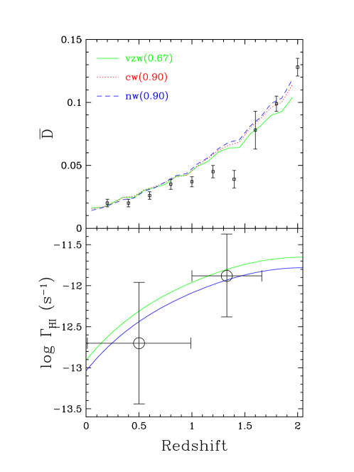
Figure 1: Top: Mean flux decrement ($\bar{D}$) evolution from $z=2\rightarrow 0$ in our three simulations. Data points are from Kirkman et al. (2007). The numbers in parantheses are the values of $f_{\tau}$ by which the optical depths are multiplied in each simulation to obtain the agreement with data as shown. Bottom: $\Gamma_{\rm HI}$ evolution that matches the mean flux for the vzw (green) and nw (blue) runs. The cw run (not shown) is identical to nw. These are simply the Haardt & Madau (2001) values divided by $f_{\tau}$. Data points show proximity effect measurements from Scott et al. (2002).

The shape and amplitude of the metagalactic photoionizing flux are still not well constrained, particularly at lower redshifts. We assume that the flux is spatially-uniform, which is probably a good approximation in the diffuse and optically thin Ly$\alpha$ forest. We take the spectral shape from that predicted by Haardt & Madau (2001) using the population of observed quasars and star-forming galaxies (their “Q1G01” model). This model assumes a 10% escape fraction of ionizing radiation from galaxies and is broadly consistent with available constraints (e.g. Scott et al., 2002).

Figure 2: Example of a section of noise-free simulated spectra ($\Delta z=1$), with an expanded region shown on the right, comparing three of our outflow models. Top panel shows Ly$\alpha$ absorption, middle shows density relative to the cosmic mean, and bottom shows temperature. The color code is nw (blue) plotted on bottom, cw (red) above, and vzw (green) on top; e.g. regions where only green shows means the others are identical to within the display resolution. The density structure is similar in all models, with the vzw having slightly more absorption overall. The cw model clearly produces a warmer IGM and the most deviations in optical depth; the other two show smaller differences.

We adjust the amplitude of the metagalactic flux to match the observed evolution of the mean flux decrement ($\bar{D}$) in the Ly$\alpha$ forest. A modest post-processing adjustment recovers essentially the identical answer to running the entire simulation with a different ionizing background, since the dynamics of Ly$\alpha$ forest gas are negligibly affected by photoionization (Weinberg et al., 1998). The amount of adjustment varies slightly among our simulations, since the outflows have a small but non-negligible impact on the Ly$\alpha$ forest. In practice, we multiply all the optical depths by a factor $f_{\tau}$ before we convert to flux, then measure $\bar{D}$, and iteratively adjust $f_{\tau}$ until we obtain a good match to $\bar{D}(z)$. In the optically-thin approximation (excellent in this case), this procedure is equivalent to multiplying the strength of the ionizing background by $1/f_{\tau}$. While in principle we could have $f_{\tau}$ be a function of redshift, this was not seen to be necessary to within the accuracy of available data, and so we simply determine a constant $f_{\tau}$ individually for each simulation.

The resulting evolution of the mean flux decrement in the Ly$\alpha$ forest is shown in the top panel of Figure 1. The values of $f_{\tau}$ are indicated in the parentheses within the legend; they are close to unity, indicating that the original Haardt & Madau (2001) metagalactic flux amplitude is viable to within current observational uncertainties. In all cases, the resulting $\bar{D}(z)$ is a reasonable match to observations by Kirkman et al. (2007), who measured the flux decrement evolution using data compiled from Hubble’s Faint Object Spectrograph (FOS) at $z\la 1.5$ and the Keck telescope’s High Resolution Echelle Spectrograph (HIRES) at $z\ga 1.5$. The simulations appear to have a somewhat higher flux decrement at $1\la z\la 1.5$, but in this regime the low resolution of FOS and the increased blending owing to a thicker Ly$\alpha$ forest (as compared to $z\sim 0$) are more likely to result in continuum placement errors that would cause the flux decrement to be biased low. Hence we do not consider these discrepancies serious as yet, though they are worth revisiting when better data becomes available from COS.

The bottom panel of Figure 1 shows the evolution of the H i photoionization rate $\Gamma_{\rm HI}$ that yields the mean flux evolution in the top panel. Since we multiply the Haardt & Madau (2001) model by a constant factor, the shapes of the curves are identical to their model. The amplitude is multiplied by $f_{\tau}^{-1}$, so vzw is slightly higher than nw; cw is identical to nw since it has the same $f_{\tau}$. All the models are consistent with the available observational constraints as they are fairly uncertain (see Davé & Tripp, 2001, for more constraints); here we show proximity effect measurements from Scott et al. (2002). If we take the $z=1.4$ measurement of $\bar{D}$ at face value and modify $\Gamma_{\rm HI}(z)$ to match it, this would result in an increase in $\Gamma_{\rm HI}$ by 0.2 dex at $z=1.4$, and a subsequent recovery back to the original track by $z=1.6$. This would be an odd detour in its evolution, implying a peak in photoionizing flux at $z\sim 1.5$ along with a secondary peak at $z\sim 2-2.5$ as in the original Haardt & Madau (2001) evolution. In this case the peak epoch of $J_{\nu}$ would no longer correspond to the peak epoch of high-luminosity quasars, although lower luminosity quasars peaking at lower redshifts could provide a significant contribution (Shankar, Weinberg, Miralda-Escudé, 2009).

It is interesting that the constant wind and no wind cases have identical values of $f_{\tau}$, while the vzw case is lower. In the simplest view, winds tend to add energy to the IGM, resulting in less Ly$\alpha$ absorption, and hence one needs smaller optical depths and a lower $f_{\tau}$. In detail however, because $\bar{D}$ is dominated by marginally saturated absorbers, the relevant issue is whether the winds are heating gas giving rise to those absorbers in particular. It turns out that vzw, owing to its smaller wind speeds from typical galaxies, tends to deposit energy closer to galaxies where strong absorbers arise, while cw tends to deposit energy far away in more diffuse gas, as we will discuss in §3. Hence we believe that although cw adds more energy to the IGM overall, this does not impact $\bar{D}$ nearly as much as in vzw.

Figure 2 shows an example spectrum from $z=0.3-0.4$ along an identical line of sight (LOS) through our three wind simulations. The Ly$\alpha$ forest is fairly sparse at these epochs, but many very weak lines exist that could be detected given sufficient observational capabilities. The mean absorption is similar by construction, but there are distinct variations evident particularly between the cw case and the other two. The expanded segment in the right panels highlights a region that shows significant differences among all three wind models. The density structure is mostly independent of outflows, though small differences are evident, but the IGM temperature can be significantly impacted by wind energy. The constant wind case shows a higher temperature almost everywhere along the LOS, while the temperatures for vzw and nw are fairly similar. However, the fact that optical depths are not very sensitive to temperature makes these differences difficult to pick out in the observed spectra. Overall, winds do not have a strong impact on the physics or absorption properties along typical lines of sight, as we will demonstrate more quantitatively with Ly$\alpha$ absorber statistics.

3 IGM Physical Conditions

3.1 Cosmic Phase Diagram

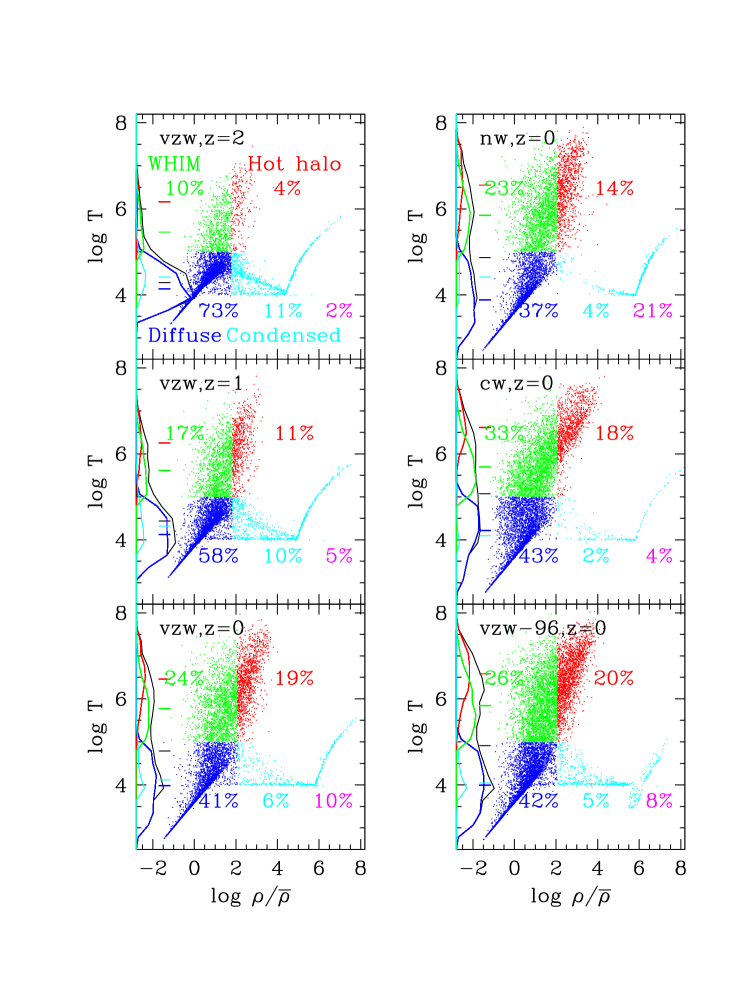
Figure 3: Left panels: Cosmic phase space diagram for gas particles in the vzw run at $z=2,1,0$ (2000 randomly-subsampled gas particles). We divide the baryons into four categories: Diffuse, Condensed, Hot Halo, and WHIM. This is done using a temperature cut at $10^{5}$ K to separate the former two from the latter two, and a density cut given by equation 1 to separate the bound baryons (condensed and hot halo gas) from the intergalactic baryons (diffuse and WHIM). Temperature histograms are along the $y$-axis for each phase and the total (black), with median values indicated by the tick marks. The percentage of mass in each phase is listed in each panel; additionally, the fraction in stars is shown in magenta. Right panels: Same, for the other simulations (nw, cw, and vzw-96), all at $z=0$.

The left panels of Figure 3 shows cosmic phase diagrams of baryons, i.e. overdensity versus temperature, in our fiducial vzw run at redshifts from $2\rightarrow 0$. The trends shown are familiar. At the lowest densities there is a tight density-temperature relation set by a competition between photoionization heating and adiabatic cooling owing to Hubble expansion. At roughly the cosmic mean density, shock heating begins on collapsing filamentary structures, creating a plume of hotter gas. At higher densities, radiative cooling becomes effective, creating the spur of dense gas that fuels star formation in galaxies. The other wind models look qualitatively similar.

Two perhaps unfamiliar features are the shelf of gas sitting at $T\approx 10^{4}$K, which is metal-enriched gas outside of star formation regions (we truncate all cooling at $10^{4}$K), and the upwards-curving plume of the densest gas, which is a consequence of the two-phase interstellar medium implementation of Springel & Hernquist (2003). The temperature in the two-phase regime is given by a mass-weighted average of the subgrid hot phase, assumed to be at $10^{8}$ K, and the mass-dominant cold phase at $1000$ K. Neither of these features are physical; they simply represent computational conveniences.

From redshift 2 to 0, we see the growth of galaxies and large-scale structure playing out in the cosmic phase diagram. The denser phases become more heavily populated, as does the plume of shock-heated WHIM gas, though the hotter phases are still clearly populated even at $z=2$. The hottest gas also grows most substantially owing to the formation of large potential wells at late times. The diffuse gas extends into lower overdensity regions at late times, as voids become more empty, and its temperature drops with time as the physical density and photoionization rates go down. The overall cosmic gas temperature distribution becomes broader with time, and shifts to slightly higher temperatures, driven by the increasing fraction in WHIM and hot halo gas. These trends have all been noted and described in previous works (e.g. Davé et al., 1999).

3.2 Redefining Cosmic Baryon Phases

In Figure 3 we have also subdivided our baryons into four cosmic phases. The subdivisions are slighly different than conventional ones (e.g. Davé et al., 2001), in which diffuse baryons are at $T<10^{5}$ K, WHIM gas is $10^{5}<T<10^{7}$ K, hot gas is $T>10^{7}$ K, and condensed baryons are at a fairly high overdensity. Our new divisions are intended to be more physically-motivated, particularly in the case of the WHIM, though in practice they do not represent dramatic changes.

The main difference is that we divide the phases according to an overdensity threshold. This threshold is intended to reflect the overdensity ($\delta\equiv\rho/\bar{\rho}-1$) at the boundary of a virialized halo. To determine this, we note that for reasonable choices of the Navarro, Frenk, & White (1996) concentration parameter $c$, the density at the virial radius is roughly one-third the mean enclosed density. We thus obtain (Kitayama & Suto, 1996)

$$\delta_{\rm th}=6\pi^{2}(1+0.4093(1/f_{\Omega}-1)^{0.9052})-1,\\$$ (1)

where

$$f_{\Omega}=\frac{\Omega_{m}(1+z)^{3}}{\Omega_{m}(1+z)^{3}+(1-\Omega_{m}-\Omega_{\Lambda})(1+z)^{2}+\Omega_{\Lambda}}.$$ (2)

$\delta_{\rm th}$ serves as our division between “bound” phases (gas in galaxies and halos) and “intergalactic” phases (WHIM and diffuse gas). The value of $1+\delta_{\rm th}$ evolves from $6\pi^{2}\approx 60$ at $1+z\gg(\Omega_{\Lambda}/\Omega_{m})^{1/3}$ to $\approx 120$ at $z=0$. This boundary is not completely sharp, as some gas that has higher overdensities is not yet bound, and owing to the elliptical nature of halos some bound gas can have lower overdensities than $\delta_{\rm th}$. We checked this definition by running a spherical overdensity halo finder (Kereš et al., 2005), and checking that equation (1) faithfully and robustly separated gas within halos from gas outside. It indeed did so, as unbound gas was never more than a couple tenths of a dex in density into the bound region, and vice versa.

We further separate the “hot” phases (WHIM and hot halo gas) from “cool phases” (diffuse and condensed gas) by a temperature threshold of $T_{\rm th}=10^{5}$ K, the same value used in earlier definitions. At high densities, all gas that is star-forming is included in the condensed phase, although the subgrid two-phase model creates a mean gas particle temperature that can exceed $T>T_{\rm th}$. At IGM densities, this represents the temperature above which the H i neutral fraction starts to drop dramatically, making Ly$\alpha$ absorption a poor tracer of its baryonic content (though as we will see later, wide Ly$\alpha$ absorbers can still trace this gas). Furthermore, since photoionization cannot easily heat gas to these temperatures, it demarcates gas that has been shock-heated by large-scale structure. From Figure 3, one can see that some gas at $T=10^{4}-10^{5}$ K is also shock-heated above the photoionization locus, but the locus itself extends to $T\approx 10^{5}$ K, at least at $z\geq 1$.

With these divisions, we have four phases as follows:

• Diffuse ($T<T_{\rm th},\delta<\delta_{\rm th}$),

• WHIM ($T>T_{\rm th},\delta<\delta_{\rm th}$),

• Hot halo ($T>T_{\rm th},\delta>\delta_{\rm th}$),

• Condensed ($T<T_{\rm th},\delta>\delta_{\rm th}$),

with the qualification that two-phase star-forming gas is “condensed” regardless of temperature. The most significant departure from previous definitions is that of the WHIM gas. Unlike the common definition in which $10^{5}-10^{7}$ K gas is WHIM regardless of density, the WHIM gas in our definition is truly intergalactic, in the sense that it is not within the boundaries of a galaxy or its halo. Also, since hot gas is most commonly detected in X-ray emission, which roughly scales as $\propto\rho^{2}T^{1/2}$ (neglecting metal line emission for the sake of this argument), this lower-density gas is more likely to be “missing” from current observational censuses. For instance, our definition removes hot gas in galaxy groups at $T\la 1$ keV from being part of the WHIM; such gas can be detected in soft X-rays (Mulchaey, 2000) because its high density (relative to truly intergalactic gas) leads to significant emission, albeit at faint levels. Hence, our revised definition more closely reflects the idea that the WHIM is the repository of the “missing” cosmic baryons. Eliminating the upper limit of $T=10^{7}$ K for the WHIM has minimal impact, since very little gas with $\delta<\delta_{\rm th}$ has such high temperatures.

3.3 Winds and the Phase Diagram

The right panels of Figure 3 show the $z=0$ cosmic phase diagram for our other simulations: nw, cw, and vzw-96. Comparing vzw-96 to vzw, we see some subtle differences particularly in the high-temperature gas. The hot halo gas extends to slightly higher temperatures, owing to larger halos being able to form in the $96h^{-1}{\rm Mpc}$ volume; this causes a slightly higher median temperature for this phase, from $10^{6.46}$ K to $10^{6.55}$ K. Similarly, the WHIM gas extends to slightly higher temperatures, causing a comparable increase in median WHIM temperature. The cooler phases show no appreciable physical differences. There is also a feature in the condensed phase at $\rho/\bar{\rho}\approx 10^{6}$ corresponding to a slightly different implementation of the two-phase cutoff in this run, but this does not affect any of our results.

The no-wind case also shows some differences with respect to vzw. Although the distribution of WHIM gas in phase space is similar, the median temperature increases slightly from $10^{5.77}$ K to $10^{5.85}$ K, just as in the vzw-96 case but for a different reason. Here, the main effect is that with no outflows, the IGM is almost completely unenriched (Oppenheimer & Davé, 2008). Hence there is no metal cooling in this regime, which yields somewhat higher temperatures. For the same reason, the condensed phase shows almost no particles at the $10^{4}$ K metal cooling floor.

The constant wind model noticeably pushes WHIM gas into a lower-density regime compared to vzw, but its median temperature is lower ($10^{5.69}$ K) since the diffuse IGM is more enriched (Oppenheimer & Davé, 2006). In contrast, the hot phase temperature is higher by $\approx 0.15$ dex, reflecting the significant IGM heating that occurs when winds from all galaxies, even small ones, are emanating at $680\;{\rm km}\,{\rm s}^{-1}$. These results are qualitatively similar to those from Tornatore et al. (2010) who explore a similar wind model, and they further note that black hole feedback (as they implement it) causes even more heating of particularly low-density gas. It is also similar to results from mesh hydrodynamic simulations by Cen & Ostriker (2006), who found that winds increase the mass fraction in the WHIM by 20%. Hence, it is possible to non-trivially impact the cosmic distribution of baryons in phase space with plausible outflows.

3.4 Baryon Phase Evolution

Figure 4: Top left: Evolution from $z=4\rightarrow 0$ of baryon fraction in various cosmic phases, including stars, in our fiducial vzw run. Next 5 panels: Evolution of baryon fraction in stars (upper right), and then the various baryonic phases in order of their location in $\rho-T$ space: WHIM (middle left), hot halo (middle right), diffuse (lower left), and condensed (lower right), in our three wind models (green, blue, red lines), along with the larger-volume vzw-96 simulation (cyan).

We now quantify the trends in the cosmic phase diagram by examining the evolution of baryons in each phase amongst our various simulations. As is apparent from Figure 3, baryons progressively move from the diffuse phase into WHIM and hot halo gas, owing to the hierarchical growth of large potential wells. The condensed phase gas is supplied predominantly from cold mode accretion but also some cooling from halo gas (Kereš et al., 2009), and this provides the fuel to grow the cosmic stellar content. By $z=0$, baryons are comparably divided between diffuse, WHIM, and the various bound phases, as was found in Davé et al. (2001). However, the new definition of the WHIM yields somewhat less WHIM gas and more diffuse gas, tilting the balance towards diffuse gas overall. The precise balance between the diffuse and WHIM phases is also sensitive to the adopted value of $T_{\rm th}$, as one can see from Figure 3.

Figure 4, top left panel, shows the fraction of baryons in each cosmic phase from $z=4\rightarrow 0$ in our vzw run. We additionally show the evolution of baryons in stars. Qualitatively, the behavior is very similar to that seen in all cosmological hydrodynamic simulations (Davé et al., 2001), as discussed above. The next five panels of Figure 4 show a comparison of individual phase evolution for our three wind prescriptions, plus our large-volume vzw-96 run. The upper right panel shows the evolution of the global stellar content, i.e. the integral of cosmic average star formation rate density vs. redshift (Madau, 1998), in each wind run. Note that these values account for stellar evolution which returns material back into the gas phase. The no-wind case produces by far the most stars, which is the well-known result that without strong feedback, there is a severe overcooling problem (Davé et al., 2001). A stellar baryon fraction today of $\sim 20\%$ far exceeds current observational values of $<10\%$ (e.g. Bell et al., 2003). Though we don’t show it here, this case is also poorly resolution-converged, as pointed out by Balogh et al. (2001), and hence the problem would be worse at higher resolution.

By contrast, both wind models do a good job of suppressing star formation. Their globally averaged star formation rates are almost identical down to $z\sim 2$, which is by design as the wind prescriptions are tuned to reproduce the observed star formation rates up to this epoch. At lower redshifts, there start to be greater differences. Because the vzw model has more recycling of wind material back into galaxies, it provides more fuel for late-time star formation (Oppenheimer et al., 2010). None of our simulations includes a prescription (e.g., AGN feedback) to truncate star formation in the most massive systems as observed, which would lower the predicted stellar fractions particularly at late times. The resolution dependence of global star formation is mitigated by the presence of outflows, as shown by Springel & Hernquist (2003b) for the cw case, and as shown here by comparing vzw and vzw-96. Both wind models are generally consistent with the currently favoured values of the stellar baryon content today of $4-8\%$ (Baldry, Glazebrook, & Driver, 2008).

The middle left panel shows WHIM evolution, which displays significant variations, particularly between models with and without galactic winds. The modest wind speeds of the vzw model do not heat much gas to WHIM temperatures compared to the purely gravitational (nw) case, but there is still some heating evident at high-$z$, which diminishes to $z=0$. The cw case shows a significant amount of WHIM gas even at $z=4$, and the WHIM fraction increases faster than in the other cases down to $z\sim 1$. At this point the supply of wind energy abates, and the WHIM fraction levels off and actually falls slightly to $z=0$. Tornatore et al. (2010) found less dramatic effect on the WHIM fraction with similar simulations, although the energy input from their winds is half of ours. These differences highlight an important point: galactic winds can in principle have a strong effect on the evolution of WHIM gas. The winds in our favoured model do not substantially affect the WHIM, but faster winds in plausible variant models can do so. Measuring the evolution of the global WHIM content could provide constraints on the large-scale thermal impact of outflows. Such measurements will be challenging given the difficulty of quantifying the WHIM even at the present epoch, but the redshifting of some UV tracer lines to longer wavelengths could potentially facilitate such measurements.

The middle right panel shows hot bound gas evolution. In general this is dominated by gravitational heating from large potential wells, as indicated by the no-wind model. The vzw case produces more hot bound gas at late times, as it removes material from galaxies and places it into their surrounding hot halos. Since the wind speed scales with escape velocity, large galaxies can have outflow velocities that exceed the wind speed of the cw model, which provides greater heating in their large halos. The cw model removes a significant amount of hot gas at early times because its high-speed winds can escape smaller potential wells, but at late times the potential wells become deep enough to retain the gas, and its hot phase rises more quickly. Still, even by $z=0$ this model does not produce as much hot bound gas as the vzw model. The vzw-96 and vzw simulations are very similar again, showing that simulation volume effects are not important even for large potential wells in terms of their global mass content.

In the lower left panel, the diffuse phase shows similar trends in all the models. The vzw winds have little impact on the diffuse gas content, as their typically modest velocities do not produce substantial IGM heating. The cw winds lower the diffuse gas fraction at high-$z$ by shock heating some IGM gas above $10^{5}$ K. This heating produces noticeable broadening of high-$z$ metal lines, leading to worse agreement (relative to vzw) with observed C iv line widths (Oppenheimer & Davé, 2006). At late times, heating of the low density IGM declines because of the reduced global star formation and the trapping of the constant-$v_{w}$ winds by deeper potential wells, causing the diffuse phase fraction to return to the no-wind value by $z\sim 0.5$. The box size has a negligibly small impact on this phase — the cyan vzw-96 curve is hidden by the overlaid green vzw curve at all but the highest redshifts.

The bottom right panel shows the condensed phase evolution. The overall trend for this phase is to increase at early epochs as material accumulates in halos, then decrease towards later times as galaxies convert gas to stars more rapidly than they accrete fresh gas. The fraction of condensed gas is $\la 10$% at all times and $\la 6\%$ today, in all the models. The cw model shows a fixed offset to lower condensed gas fractions relative to the no-wind model, since it expels a constant amount of material out of the star-forming regions, and most of this material ends up outside of halos owing to the large wind speed. The vzw model shows qualitatively different behavior from the others, with less redshift evolution. Mostly this difference reflects the late-time reaccretion of wind material, more prominent in the vzw model because of lower wind speeds (Oppenheimer et al., 2010). We note the qualitative similarity of the evolution of this phase (which contains most of the cosmic neutral gas) with the observed evolution of cosmic H i gas from Damped Ly$\alpha$ systems (Wolfe et al., 2005), being roughly constant from $z\sim 3\rightarrow 0.5$ and then dropping to $z=0$.

Returning to Figure 3, the histograms along the vertical axis show the temperature distribution of baryons at $z=2,1,0$. The overall trend follows the movement of baryons within the cosmic phase diagram, namely that the median temperature increases with time. In detail, the diffuse phase actually moves towards lower temperatures because of the changing balance between photionization heating and adiabatic cooling. The WHIM gas extends up to higher temperatures at low-$z$, and the hot bound gas also becomes hotter on average as larger potential wells form. The median cosmic gas temperature today is $\approx 10^{5}$ K.

Overall, the cosmic evolution of baryon phases reflects the hydrodynamic and radiative processes associated with the growth of structure. Winds have a significant impact, particularly on the stellar phase (by design) and on the WHIM phase (if the winds are strong enough). They also impact the bound phases (hot halo and condensed), since these lie close to galaxies where winds play a more important dynamical role. The diffuse phase is mostly unaffected by winds. The complex dynamical interplay between outflows and hierarchical growth is an important factor in the cosmic history of baryons, and improved observational constraints and theoretical predictions will be required to fully characterise it.

4 Ly$\alpha$ Absorber Observables

We now investigate the statistics of Ly$\alpha$ absorbers in our simulated COS-like spectra, and present comparisons when appropriate to existing pre-COS data. We consider the canonical statistics of the column density and linewidth distributions, as well as the evolution of the number density of lines. To obtain line statistics, we fit our simulated spectra with Voigt profiles using AutoVP (Davé et al., 1997), yielding an H i column density ($N_{\rm HI}$), Doppler line width ($b$), and redshift for each absorber. Owing to the sparseness of the low-$z$ Ly$\alpha$ forest, the fits are generally unambiguous, and tests have shown that AutoVP obtains line parameters very similar to that from other Voigt profile fitters (e.g. VPFIT) when the lines are unsaturated. We use the continuum directly provided by the simulations, as we assume that observed spectra can be fit with an accurate continuum in the relatively sparse low-$z$ Ly$\alpha$ forest. We also examine the impact of varying the assumed signal-to-noise ratio and spectral resolution of our simulated spectra. Note that AutoVP provides “raw” $b$-parameters uncorrected for instrumental resolution. In our COS-resolution spectra, with a Gaussian width of $17\;{\rm km}\,{\rm s}^{-1}$, we therefore expect essentially no lines with $b<17\sqrt{2}\approx 24\;{\rm km}\,{\rm s}^{-1}$. Since it turns out that the vzw-96 absorber statistics are indistinguishable from the vzw case (as anticipated by the close agreement in IGM physical properties), we do not show this model herein.

4.1 Column Density Distributions

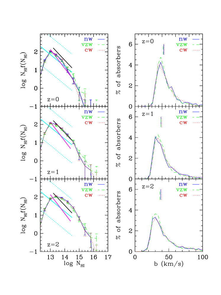
Figure 5: Column density (left) and $b$-parameter (right) distributions at $z=0$ (top), $z=1$ (middle), and $z=2$ (bottom) for our three simulations. The CDD have been multiplied by $N_{\rm HI}$ improve visibility of the differences between models. The thick cyan line shows a fit to data from Penton, Stocke, & Shull (2004) at $z\approx 0$, namely $\log f(N_{\rm HI})=10.3-1.65\log{N_{\rm HI}}$, over their fitted range of $12.3\leq\log{N_{\rm HI}}\leq 14.5$; dotted lines on either side indicate their $1\sigma$ quoted uncertainty of $\pm 1.0$ in $\log f(N_{\rm HI})$. Thick black and magenta lines show best fits for CDDs from STIS data from Lehner et al. (2007) and Davé et al. (2001), respectively. The same lines are reproduced at the other redshifts for reference, showing that there is modest evolution in the CDD amplitude from $z=2\rightarrow 0$. The turnover at $N_{\rm HI}<10^{13}{\rm cm}^{-2}$ arises from incompleteness in recovering lines at the assumed S/N and resolution; see §4.4. Linewidth distributions are shown for all lines with $N_{\rm HI}>10^{13}{\rm cm}^{-2}$, i.e. our complete sample at COS resolution and an assumed S/N=30. Tick marks above each curve indicate median $b$ values.

Figure 5 shows column density (left panels) and $b$-parameter (right panels) distributions for absorbers at $z=0,1,2$. As mentioned previously, these three bins correspond to all lines within redshift ranges $z=0-0.2$, $z=0.9-1.1$, and $z=1.8-2$, respectively, identified with AutoVP in our 70 random lines of sight. Results are shown for all three of our outflow models. The column density distribution (CDD) $f(N_{\rm HI})\equiv d^{2}N/dN_{\rm HI}dz$ has been multiplied by $N_{\rm HI}$ to remove some of the steep power-law scaling (discussed below), which enhances the visibility of the differences among models. It also results in a dimensionless number that reflects the relative number of lines per unit redshift at a given $N_{\rm HI}$.

The CDD shows the usual power-law behaviour, above the completeness limit at $N_{\rm HI}\approx 10^{13}{\rm cm}^{-2}$ that results from our adopted S/N and resolution (see §4.4). Characterizing the column density distribution as a power law with $f(N_{\rm HI})\propto N_{\rm HI}^{-\beta}$, and fitting between $10^{13}<N_{\rm HI}<10^{14.5}{\rm cm}^{-2}$, we obtain values of $\beta=-1.88,-1.70,-1.80$ for the nw, vzw, and cw models at $z=0$, respectively, with an uncertainty of approximately $\pm 0.1$ on each. Hence, all the slopes are formally consistent with each other, although given that the exact same LOS are being analyzed, one can conclude that the nw model produces a steeper slope than the wind models, and that the vzw model produces the shallowest slope. We note that all the slopes are shallower than the slope $-2.04\pm 0.23$ obtained in the simulation by Davé et al. (2001) (though within formal uncertainties), which was most analogous to the no-wind case here. We will show in §4.4 that higher spectral resolution tends to produce a somewhat steeper slope, so this could explain part of the difference. Paschos et al. (2009) found a slope of $-1.84\pm 0.02$ using a fixed mesh simulation with 75 kpc resolution and no galactic outflows, which basically agrees with our no-wind case.

These are several pre-COS set of low-$z$ Ly$\alpha$ forest data for comparison. One sample, from Penton, Stocke, & Shull (2004), contains 187 somewhat heterogeneous Ly$\alpha$ absorbers, mostly at $z\la 0.1$, from Hubble/STIS and Goddard High Resolution Spectrograph data. A more uniform and higher-resolution sample of 341 absorbers out to $z\la 0.4$ was obtained by Lehner et al. (2007) using only STIS data, and included Far Ultraviolet Space Explorer data to help constrain the properties of saturated Ly$\alpha$ absorbers. We also show earlier results from Davé et al. (2001), who analyzed two STIS spectra using AutoVP. The fits to all their resulting CDDs are shown as the thick lines in the upper left panel of Figure 5; black for Lehner et al. (2007), magenta for Davé et al. (2001), and cyan with $\pm 1\sigma$ uncertainties shown as the dashed lines for Penton, Stocke, & Shull (2004). The slope obtained by Penton, Stocke, & Shull (2004) is $-1.65\pm 0.07$, which is statistically different from that of Lehner et al. (2007) ($-1.84\pm 0.06$) or Davé et al. (2001) ($-2.04\pm 0.23$). As we will show in §4.4, at least part of the difference likely owes to spectral resolution, since higher resolution data yields steeper slopes. For this reason it is not straightforward to compare to the COS predictions presented here to these data, but broadly the slope and amplitude predicted by the current simulations are in agreement given the various uncertainties. A careful comparison against upcoming COS data should provide more discrimination between models.

At higher column densities, Penton, Stocke, & Shull (2004) found that their data showed a characteristic “dip” in the CDD at $N_{\rm HI}\sim 10^{15}{\rm cm}^{-2}$, which they point out persists from high-$z$ (see their Figure 9). Lehner et al. (2007) likewise saw that the CDD slope is shallower at $N_{\rm HI}>10^{14.4}{\rm cm}^{-2}$ than for smaller systems. We see a hint of the onset of such a dip in all our simulations, but we cannot accurately trace it out to $N_{\rm HI}\ga 10^{16}{\rm cm}^{-2}$, since we quickly run out of absorbers owing to the rarity of high-$N_{\rm HI}$ absorbers along our randomly-chosen LOS. The origin of this dip is unclear. It occurs at a column density close to that expected for overdensities near the boundaries of galaxy halos, which leads us to speculate that perhaps these absorbers probe the outer parts of galaxy halos where (at least in larger halos) some of the gas might be shock-heated to a temperature where it would not absorb in H i. At even higher columns, one would then probe through denser halo regions where H i condenses out again, owing to self-shielding, causing a “recovery” back to the original CDD. We leave a detailed examination of this conjecture for future work.

The redshift evolution of the CDD shows a steady march upwards in line counts at a given $N_{\rm HI}$ ($\ga 10^{13.5}{\rm cm}^{-2}$). The overall steady evolution reflects the evolution of the mean flux decrement over this redshift range, and hence is dependent on our procedure of adjusting the ionizing background strength to match $\bar{D}(z)$. The incompleteness at $N_{\rm HI}\la 10^{13.5}{\rm cm}^{-2}$ becomes more severe at higher-$z$, as line blending becomes more common. Recall that we have fixed our resolution and line spread function to the COS far-UV channel at all $z$, which underestimates the data quality that is obtainable at $z\sim 1$ (where the COS NUV channel has a narrower LSF, albeit with lower sensitivity) and at $z\sim 2$ (where one can trace the Ly$\alpha$ forest in the optical). This makes it difficult to compare slopes across a fixed $N_{\rm HI}$ range, but if we restrict ourselves to $10^{13.4}-10^{14.6}{\rm cm}^{-2}$ where the CDD is reasonably complete at all $z$, we obtain slopes for the vzw model of $-1.89,-1.71$, and $-1.54$ at $z=0,1,2$, respectively. The CDD is clearly getting steeper with time, broadly matching the observed CDD slope evolution from high-$z$ ($\sim-1.5$, e.g. Kim, Cristiani, & D’Odorico, 2001; Janknecht et al., 2006) to low-$z$.

The CDDs are remarkably insensitive to the outflow model at lower column densities. Wind dynamics, despite enriching the IGM and depositing energy over large scales in quite different ways, have little impact on the diffuse H i distribution. As shown by Oppenheimer & Davé (2008) and Kollmeier et al. (2003, 2006), the typical extent of galactic winds ($\sim 100$ kpc physical) generally does not extend into the diffuse Ly$\alpha$ forest. This was noted in the earliest simulation studies of Ly$\alpha$ absorption that explored outflows Theuns et al. (2002). However, there are significant differences for stronger absorbers, as outflows (particularly in the vzw case) deposit more cool gas in the outskirts of halos, which increases the Ly$\alpha$ absorbing cross-section. This yields significantly more sub-Lyman Limit systems and slightly shallower CDD slopes, and it is also reflected in the number counts of strong lines as we will show in §4.3.

4.2 $b$-parameter Distributions

The right panels of Figure 5 show the $b$-parameter distributions for our three wind models at $z=0,1,2$. The histograms show the usual Gaussian distribution with an extended tail to higher line widths. The median $b$-parameter for each model is indicated by the tickmark above the curves. The typical value is around $40\;{\rm km}\,{\rm s}^{-1}$ at all $z$, with a slight trend to become smaller at high-$z$.

The line widths are significantly wider than what was found using STIS data (e.g. Davé et al., 2001; Williger et al., 2010). Simulations by Davé et al. (2001) predicted a median $b$ that depended on $N_{\rm HI}$ with a typical value of $25\;{\rm km}\,{\rm s}^{-1}$, in good agreement with their STIS data. Lehner et al. (2007) determined a median $b=30\;{\rm km}\,{\rm s}^{-1}$, also from STIS data. Paschos et al. (2009) used simulated spectra with approximately $5\;{\rm km}\,{\rm s}^{-1}$ resolution and obtained a similar $b$-parameter distribution. We will show in §4.4 that the larger $b$ values predicted in this work are mostly a result of the poorer spectral resolution of COS relative to STIS. Our simulated line widths are more comparable to those obtained using GHRS ($\sim 18\;{\rm km}\,{\rm s}^{-1}$ resolution; Penton, Stocke, & Shull, 2004). Owing to this sensitivity to instrumental characteristics, we do not conduct any detailed comparison with data here. Nevertheless, we will show in §5 that line widths still contain some information about the underlying temperature of the absorbing gas. It may be possible to extract better constraints on linewidths using higher-order Lyman lines through a curve-of-growth analysis or through simultaneous fitting of multiple transitions (e.g. Lehner et al., 2007), but we leave such a study for the future.

The line widths, like the CDDs, show almost no sensitivity to outflow model. This is perhaps more surprising, given that the various wind models heat the IGM to different levels (see Figure 4), with cw clearly providing substantial heating. In §5.4, we will show that the $b$ parameters are only loosely correlated with temperature, reflecting the dominance of other sources of line broadening such as Hubble flow and instrumental resolution. In detail, the cw model does have marginally higher median $b$ values of 43.0, 39.4, and $38.2\;{\rm km}\,{\rm s}^{-1}$ at $z=0,1,2$ respectively, as compared to vzw which has 42.3, 38.2, and $36.2\;{\rm km}\,{\rm s}^{-1}$ (almost identical to nw), so the expected effect is present but small. We will also show in §4.4 that $b$ parameters are highly sensitive to spectral resolution, and hence comparisons of data to models (or to other data sets) must carefully account for such effects.

4.3 Absorber Evolution

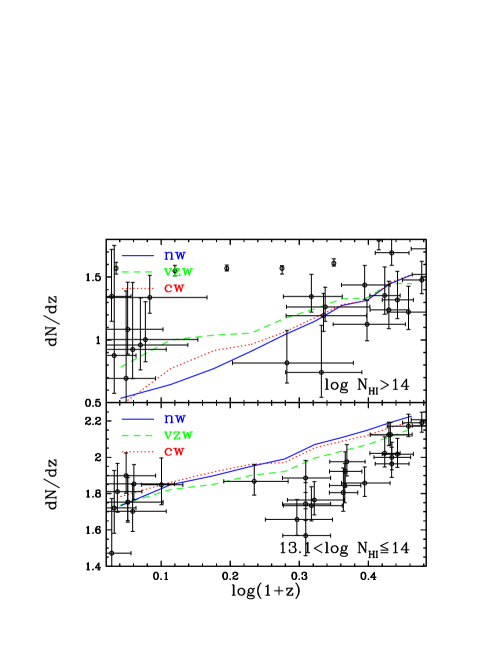
Figure 6: Line-of-sight number density of Ly$\alpha$ absorbers ($dN/dz$), as a function of redshift. Top panel shows the evolution of absorbers with $N_{\rm HI}>10^{14}{\rm cm}^{-2}$, while bottom panel shows $10^{13.1}<N_{\rm HI}\leq 10^{14}{\rm cm}^{-2}$. Data from various sources compiled by Williger et al. (2010) are indicated.

The evolution of Ly$\alpha$ absorbers provides insights into the interplay between cosmic expansion, photoionization, and the growth of structure. One simple statistical characterization of this evolution is the redshift-space number density of absorbers along the line of sight, $dN/dz$.

$dN/dz$ is usually measured within a specified column density range. Early data from FOS (Weymann et al., 1998) showed a dramatic change in the evolution rate of strong ($N_{\rm HI}\ga 10^{14}{\rm cm}^{-2}$) absorbers between $z\ga 2$ and $z\la 1$. However, subsequent higher-quality data has muddled the situation. Owing to the paucity of such strong absorbers, there appears to be substantial cosmic variance for $dN/dz$ among the various sightlines. Moreover, more recent data with substantially higher resolution generally shows a significantly lower $dN/dz$ compared to the FOS results, presumably because higher resolution enables more accurate deblending of strong lines. It appears that large redshift path length and high spectral resolution are both necessary to obtain an accurate estimate of $dN/dz$ for strong absorbers; COS should provide this combination.

Figure 6 shows the evolution of $dN/dz$ for our three outflow models. The top panel shows $dN/dz$ for $N_{\rm HI}>10^{14}{\rm cm}^{-2}$ lines, while the bottom shows $10^{13.1}<N_{\rm HI}\leq 10^{14}{\rm cm}^{-2}$ absorbers. Overlaid are a compilation of data taken from Williger et al. (2010). For strong lines, the points across the top of the panel are the Key Project FOS results (Weymann et al., 1998). The others come from higher-resolution data sets, and are all significantly lower than the FOS results. In general, the simulations show a relatively slow decline in $dN/dz$, with little evidence for any kind of “break” in evolution as was seen in the FOS data. Theuns, Leonard, & Efstathiou (1998) and Davé et al. (1999) emphasized that the decline of the UV background at $z<2$ slows the evolution of the forest relative to a constant UVB case. The steadiness of evolution in Figure 6 relative to Figure 3 of Davé et al. (1999) is partly a consequence of the narrower redshift range and partly a consequence of adopting a UVB that declines more slowly at low redshift because of contributions by galaxies.

The strong absorbers show a clear discrimination between outflow models by $z=0$, with twice as many $N_{\rm HI}>10^{14}{\rm cm}^{-2}$ absorbers in the vzw model as in the no-wind case. The cw model is intermediate. This shows that our favoured outflow model is ejecting more gas into the vicinity of galaxies where strong absorbers arise, and that this gas is remaining relatively cool. The difference arises because the momentum driven wind model ejects more material from lower-mass galaxies at lower wind speeds, thereby providing a reservoir of cooler gas that can cause strong Ly$\alpha$ absorption. This is qualitatively the same effect that causes this model to provide a larger amount of DLA absorption and broader DLA kinematics, as described by Hong et al. (2010). The vzw case shows the best agreement with recent $z\sim 0$ data, which is directly tied to its somewhat shallower CDD slope, although the uncertainties are still large enough to preclude any firm discrimation. COS should yield a good observational determination, providing an important diagnostic of galactic outflows.

The weaker absorbers show much less sensitivity to outflows, indicating that winds do not substantially disturb gas at the densities giving rise to $N_{\rm HI}\la 10^{14}{\rm cm}^{-2}$ absorbers. A reasonable fit for all the models is given by $dN/dz\propto(1+z)^{0.7}$, which is significantly shallower than the evolution at high-$z$ (e.g. Davé et al., 1999). However, all the models generically fail to reproduce the apparent break in evolution at $z\sim 1$ (Janknecht et al., 2006). This can be traced directly to the evolution of the mean flux decrement $\bar{D}$ (Figure 1), which the models overpredict around $z\sim 1$ by the same factor of two that they ovthe erpredict $dN/dz$. In fact, the two observational data sets are not unrelated, as $\bar{D}$ is most sensitive to absorbers just below the logarithmic portion of the curve of growth, namely $N_{\rm HI}\la 10^{14}{\rm cm}^{-2}$. If we adjusted the UVB intensity to reproduce the Kirkman et al. (2007) $\bar{D}$ measurements at $z=1-1.5$, then we would predict a break in $dN/dz$ evolution at $\log(1+z)\approx 0.35$. Improved statistics will thus provide valuable constraints on the evolution of the UVB, perhaps demonstrating significant departures from the Haardt & Madau (2001) predictions.

In summary, the evolution of Ly$\alpha$ absorbers will in principle provide strong constraints on the evolution of the ionizing background (for weaker lines), and perhaps on the nature of outflows (for stronger lines). However, accurate constraints require larger data sets with good resolution, which COS should provide.

4.4 The Effects of Instrumental Resolution and Noise

Intrumental resolution and noise characteristics of the data can have a non-trivial impact on the derived statistics of Ly$\alpha$ absorbers. This can lead to some confusion when cross-comparing different samples, or when comparing simulations to data without carefully matching such characteristics. In this section we use our simulations to briefly investigate how COS-resolution data would compare to an equivalent sample of higher STIS-resolution data, and how the Ly$\alpha$ forest would appear if it were possible to greatly boost the S/N of COS data. These are idealized experiments, not readily achievable with current instruments, but they illustrate the trends one should keep in mind when intercomparing samples.

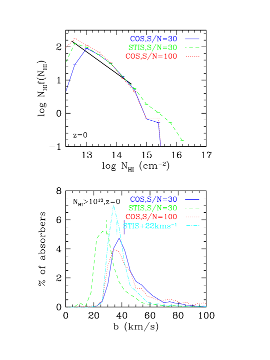
Figure 7: Effects of signal-to-noise ratio and spectral resolution on Voigt profile parameter distributions in our fiducial vzw run at $z=0$. COS resolution assumes the COS LSF in the FUV channel, which is $\approx 17\;{\rm km}\,{\rm s}^{-1}$ Gaussian width ($1\sigma$), while STIS resolution assumes a Gaussian with $7\;{\rm km}\,{\rm s}^{-1}$ width. Top panel shows column density distributions multiplied by $N_{\rm HI}$, demonstrating that the turnover at low-$N_{\rm HI}$ at $10^{13}{\rm cm}^{-2}$ owes to a lack of sensitivity; either increasing S/N or resolution allows one to probe further. There are also differences at the high-$N_{\rm HI}$ end. Bottom panel shows the $b$-parameter distributions; these are not very sensitive to S/N variations, but are dramatically sensitive to spectral resolution. Here we also show the result of convolving the linewidths identified in the STIS-resolution spectra with a 22 km/s Gaussian to illustrate the effect of moving from STIS to COS resolution; this demonstrates that much of the line broadening in the COS-resolution case owes to its coarser spectral resolution.

Figure 7 shows the CDD and $b$-parameter distributions for the vzw model at $z\approx 0$ for our simulated spectra convolved with a COS LSF at S/N=30 and 100, and with a $7\;{\rm km}\,{\rm s}^{-1}$ Gaussian (with $3\;{\rm km}\,{\rm s}^{-1}$ pixels) intended to roughly mimic STIS resolution. The higher S/N or resolution both extend the CDDs to lower column densities with an unbroken power law, showing that our COS-resolution sample with S/N=30 is essentially complete to $N_{\rm HI}=10^{13}{\rm cm}^{-2}$. Coincidentally, increasing the S/N to 100 at COS resolution is roughly equivalent, in terms of CDD completeness, to having STIS resolution with S/N=30. At the high-$N_{\rm HI}$ end, STIS resolution produces quite a few more strong lines. We caution that different Voigt profile fitting algorithms can significantly affect the parameters derived for saturated lines, so one must be careful in interpreting this plot. However, it does indicate that some of the variations seen in $dN/dz$ for strong lines may owe to different instrumental characteristics for the various data sets. Examination of the true column densities in the simulated absorbers shows that the high column density systems identified in the STIS-resolution spectra are generally real; at COS resolution AutoVP mischaracterizes them as lower column density systems with larger $b$-parameters (and thus less saturation). Finally, the slope of the CDD at $10^{13}<N_{\rm HI}<10^{14.3}{\rm cm}^{-2}$ is steeper in the case of higher S/N or resolution; for the former, we obtain a slope of $-1.73$ (as opposed to $-1.70$ for the original vzw case), and for the latter we get $-1.82$. Hence, high resolution produces a significantly steeper CDD slope, which can help explain why the CDD slopes in Davé & Tripp (2001) are steeper.

The $b$-parameter distribution shows strong sensitivity to spectral resolution, but increasing S/N does not have a major impact on $b$ parameters. At STIS resolution, the median $b$-parameter is below $30\;{\rm km}\,{\rm s}^{-1}$, and the distribution roughly agrees with that found in Davé et al. (2001). At COS resolution, lines are significantly broader, resulting in a median greater than $40\;{\rm km}\,{\rm s}^{-1}$ and a much more prominent tail to high $b$ values. The cyan dot-dashed curve in Figure 7 shows the result of taking each line in the STIS-resolution distribution and increasing its $b$-parameter by adding $\sqrt{2(17^{2}-7^{2})}\approx 22\;{\rm km}\,{\rm s}^{-1}$ in quadrature to account for the difference in resolution between COS and STIS. The peak of the distribution moves much closer to that of the COS distributions, suggesting that for many lines the larger COS $b$-parameter is a simple consequence of convolving the line with a broader LSF. However, the COS distributions still have many more lines at $b\geq 60\;{\rm km}\,{\rm s}^{-1}$, showing that these broad lines must arise mainly from blends that cannot be resolved by the COS FUV channel. Because of the effects of line-blending, we think it is generally better to test models by applying the LSF to simulated spectra rather than attempting to correct measured $b$-parameters on a line-by-line basis. The exception might be in cases where higher order Lyman series lines provide additional constraints on the $b$-parameters via curve-of-growth analysis. More generally, this illustrates that the $b$ parameters are particularly sensitive to spectral resolution, and any comparisons between data sets, or between data and models, should take special care to match the instrumental line spread function.

5 Ly$\alpha$ Absorber Physical Conditions

We now examine the relationship between absorber properties and the physical conditions of the absorbing gas, namely its temperature, density, and ionization state. The relatively simple nature of Ly$\alpha$ forest absorption, particularly for weaker absorbers, results in fairly tight relationships that offer insights into the evolution of baryons in the IGM.

To assign densities and temperatures to individual absorbers, we find the location of peak absorption and assign to the absorber the H i-weighted $\rho$ and $T$ of the nearest pixel. This is not a perfect procedure, as, e.g., the width of the line might be determined by coincident hotter gas superposed on stronger absorption from colder gas. But it gives a reasonable idea of the physical conditions present in the absorbing gas. To better isolate real trends, we only consider absorbers whose formal $\chi^{2}$ errors for $N_{\rm HI}$ and $b$ as reported by AutoVP are fractionally less than 20%, which mostly removes very weak absorbers whose parameters are not well-determined. For studying linewidths, we include only absorbers with $N_{\rm HI}>10^{13}{\rm cm}^{-2}$, for which we have a relatively complete sample. We focus on the momentum-driven wind case and point out where substantial differences arise in the other wind models.

5.1 Absorbers in Phase Space

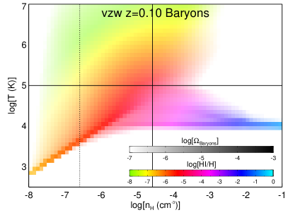
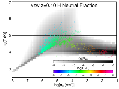
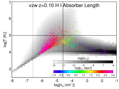
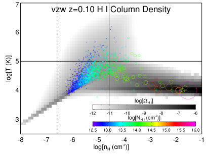
Figure 8: Cosmic phase diagrams for the vzw run at $z=0.1$. Upper left shows all baryons, colored by H i fraction. Other panels are shaded by $\Omega_{HI}$, binned in $0.1\times 0.1$ dex pixels. Solid lines demarcate the four cosmic phases as in Figure 3, while the dotted line indicates the cosmic mean density. In each panel, the circles show the locations of $z=0-0.2$ absorbers in phase space, with the area of the circle proportional to $N_{\rm HI}$ (see lower left panel for scale). The color scale in each panel corresponds to different quantities: Ionization fraction (upper right), total hydrogen column density $N_{H}$ (middle left), absorber size (middle right), $N_{\rm HI}$ (lower left) and linewidth (lower right).

Figure 8 shows how Ly$\alpha$ absorbers populate and trace cosmic phase space (here shown as temperature vs. hydrogen number density). In each panel except the upper left, our simulated absorbers between $z=0-0.2$ are indicated as circles, placed using their H i-weighted densities and temperatures. Solid lines demarcate the phase boundaries as defined in §3.2 and shown in Figure 3, and the vertical dotted line indicates the cosmic mean density of hydrogen. Our absorber sample overlaps the shading, which represents the simulated distribution of H i. However, because random sight lines sample the Ly$\alpha$ forest in a volume-weighted fashion, there are more weak Ly$\alpha$ absorbers tracing lower densities even though most of the cosmic H i resides in rare, strong absorbers tracing the condensed phase. Conversely, absorbers are not detectable at densities below $n_{H}=10^{-6}$ cm^-3, where the vast majority of the IGM volume exists, and this detectability threshold is the reason that the low-z Ly$\alpha$ forest is observed to be sparsely populated.

The upper left panel displays the cosmic distribution of baryons in phase space, color-coded by ionization fraction. The remaining 5 plots contain up to three additional dimensions of information within two-dimensional cosmic phase space: Shading for global H i content (i.e. the product of the intensity and color maps in the top left panel), circle size scaled to absorber $N_{\rm HI}$, and circle color for the various quantities, as follows: Neutral fraction (upper right), total hydrogen column (middle left), absorber path length (middle right), $N_{\rm HI}$ (lower left), and linewidth (lower right). It is clear that there are strong correlations amongst the various physical and observational quantities. In subsequent sections we will quantify some of these trends in more detail and attempt to connect observables to physical quantities within this plane.

The H i neutral fraction in the upper right panel is computed for each absorber as an optical depth-weighted neutral fraction from all SPH particles that contribute to the absorption. Note that we assume ionization equilibrium; this is expected to be a very good approximation in the Ly$\alpha$ forest. It is clear that, as expected, the IGM is highly ionized, with the weakest absorbers showing neutral fractions of $\sim 10^{-6}$ cm^-3. Neutral fractions increase towards lower temperature and higher density, such that absorbers at $\sim 10^{14}{\rm cm}^{-2}$ (the typical absorber at the crossing point of the phase division lines) show a neutral fraction of $\sim 10^{-5}$ cm^-3. The neutral fraction increases rapidly along the condensed phase, leading quickly to very strong absorbers.

The middle left panel of Figure 8 shows the total hydrogen column density $N_{H}$, computed by dividing $N_{\rm HI}$ by the neutral fraction. A remarkable trend emerges that the vast majority of Ly$\alpha$ forest absorbers have $N_{H}$ between $10^{18}{\rm cm}^{-2}$ and $10^{19}{\rm cm}^{-2}$, except for the hottest or densest absorbers. This trend was noted observationally in a small sample by Prochaska et al. (2004), which they pointed out was in general agreement with simulation predictions from Davé et al. (2001). Here the trends of $N_{H}$ versus overdensity can be more clearly seen; it is double-valued in the sense that $N_{H}$ is lower at both low and high overdensities, and it peaks at intermediate overdensities, particularly at high temperatures.

The middle right panel shows an estimated size of Ly$\alpha$ absorbers, obtained by dividing $N_{H}$ by the physical density. Weak absorbers ($\sim 10^{13}{\rm cm}^{-2}$) have sizes up to $\sim 1$ Mpc, and this quickly drops to $\sim 100$ kpc for $\sim 10^{14}{\rm cm}^{-2}$. This is broadly consistent with the large coherence lengths observed in quasar pair sightlines (e.g. Dinshaw et al., 1998; Casey et al., 2008), though the elongated geometry of absorbing structures also affects apparent coherence lengths. The sizes are consistent with analytic estimates by Schaye (2001) from assuming that Jeans smoothing establishes the structure of the low-density IGM. (See Peeples et al. [2010] for evaluation of this hypothesis against simulation results, albeit at higher redshift.) The absorber lengths drop rapidly with increasing overdensity, such that strongest absorbers in the condensed phase have sizes $\sim 1$ kpc or less. This explains why absorbers from this phase are rarely seen despite the substantial reservoir of neutral gas in the condensed phase — their cross-section is remarkably small.

The two lower panels consider absorber observables $N_{\rm HI}$ and $b$. The lowest column density systems lie along the low-density, high-temperature envelope of detectable H i. The trend of increasing $N_{\rm HI}$ towards low temperatures and high densities mimics that in the ionization fraction, such that the typical absorber at the bound/unbound division has $N_{\rm HI}\sim 10^{14}{\rm cm}^{-2}$ (and lower at higher temperatures). The strongest absorbers generally arise in condensed phase gas, though they are rare in these random LOS.

The $b$-parameters in the lower right panel also show trends in phase space, but they are not as distinct as with column densities. Narrower lines tend to arise in lower-density and lower-temperature gas, but there is a significant scatter. Wide lines can occur in hot gas, but such gas can also contain narrower lines. Wide lines can also occur in very strong absorbers that are heavily saturated, arising in condensed gas. Overall, $b$ parameters trace temperatures fairly loosely, a point we will quantify further in §5.4.

Overall, Ly$\alpha$ absorption along random lines of sight can trace present-day baryons from close to the mean overdensity up to overdensities of $\sim 10^{4}$ or more, and to temperatures well above $10^{5}$ K. There are strong trends of ionization fraction and absorber size, which together with the underlying baryon distribution in phase space yield a strong trend of physical parameters versus column density, and a weaker but still noticeable trend versus linewidths. In the next two sections we explore these trends more quantitatively, to better understand how observables obtained from COS spectra can reveal the physical conditions of the absorbing gas.

5.2 Column density versus physical density

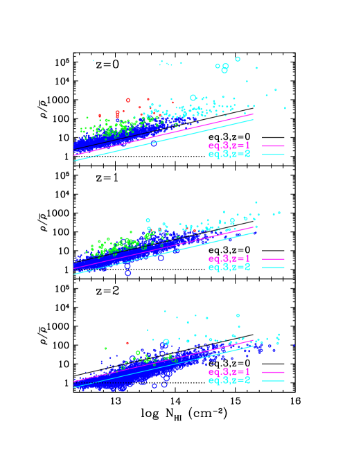
Figure 9: Baryonic physical density in units of the cosmic mean ($\rho/\bar{\rho}$) versus column density $N_{\rm HI}$ for absorbers from the momentum-driven wind model, at $z=0$ (top), $z=1$ (middle), and $z=2$ (bottom). In each panel, the solid line shows the relation from equation 3 at $z=0$ (black), $z=1$ (magenta) and $z=2$ (cyan). Absorbers are color-coded as diffuse (blue), WHIM (green), hot (red), or condensed (cyan). Point sizes are scaled $\propto b$.

The evolution in the relationship between column density $N_{\rm HI}$ and overdensity $\delta$ is governed by the interplay between cosmic expansion, which lowers the physical density (at a given $\delta$) and thus lowers the recombination rate, and evolution of the UV background, which drops at lower redshifts and thus lowers the photoionization rate. Davé et al. (1999) showed that much of the observed evolution in the Ly$\alpha$ forest can be understood through the evolution in this relation, because this interplay causes a given strength absorber to correspond to a higher overdensity at lower redshift. Complications arise because, by $z=0$, a significant amount of IGM gas is heated collisionally by shocks rather than by photoionization, resulting in departures from the FGPA (Zhan et al., 2005). Nevertheless, this $N_{\rm HI}-\delta$ relation is central to understanding the physics of the Ly$\alpha$ forest in a structure formation context.

Figure 9 shows that a fairly tight $N_{\rm HI}-\delta$ relation is established at all redshifts, as found by previous studies. The three panels show this relation for the momentum-driven wind model at $z=0,1,2$. Absorbers are categorized by cosmic phase, with a color code following Figure 4, namely diffuse (blue), WHIM (green), hot halo (red), and condensed (cyan). The lower envelope reflects gas that is purely photoionized, as shock heating will move absorbers to lower $N_{\rm HI}$ for a given overdensity by lowering the neutral fraction.

The diffuse-phase absorbers follow a tight relation in overdensity versus temperature owing to photoionization heating and cosmic expansion (Hui & Gnedin, 1997; Schaye, 2001). We perform a least-squares fit to the diffuse absorbers as a function of column density and redshift (from $z=0-2$), restricting ourselves to absorbers with $T<10^{4.5}$ K to remove mildly shocked systems, and obtain the following relation:

$$\frac{\rho}{\bar{\rho}}=\frac{35.5\pm 0.3}{f_{\tau}^{0.741}}\Bigl{(}\frac{N_{\rm HI}}{10^{14}{\rm cm}^{-2}}\Bigr{)}^{0.741\pm 0.003}10^{(-0.365\pm 0.009)z}.$$ (3)

Recall that $f_{\tau}$ is the factor by which optical depths have been multiplied relative to those computed for the Haardt & Madau (2001) ionizing background, to match the mean flux decrement; it is $2/3$ for our momentum-driven wind model. The quoted uncertainties are on means, and they do not reflect the spread amongst the individual absorbers. This fit is shown at each redshift in each panel, to help visualize the rate of evolution. Our slope for $\rho$ vs. $N_{\rm HI}$ is similar to the slope of two-thirds derived by Schaye (2001) from Jeans smoothing arguments. Furthermore, the redshift evolution is in excellent agreement with predictions from his analytic model.

The WHIM absorbers generally have somewhat higher density at a given $N_{\rm HI}$, since the gas has been shock-heated; this trend is exacerbated for the hot halo absorbers. As a result, at overdensities above 10 or so, corresponding to $N_{\rm HI}\ga 10^{14}{\rm cm}^{-2}$ at $z\sim 0$, there begin to be significant departures from equation (3). The departures from this relation also become more prominent with time, since more IGM gas becomes shock-heated. Condensed phase gas typically gives rise to the strongest Ly$\alpha$ absorption systems seen at the highest overdensities. At $z=2$ there is a shelf at the lowest densities, largely because the underdense absorbers have larger velocity widths and are thus more difficult to identify at fixed $N_{\rm HI}$ and S/N.

Equation (3) is similar in form to the (by-eye) fits presented in Davé et al. (1999) and Davé et al. (2001). Differences arise because the ionizing background strength employed here is slightly different, and here we consider only the diffuse absorbers. We have checked that the above equation holds reasonably well for the diffuse absorbers in the no wind and constant wind cases (when the $f_{\tau}$ factor is included), since these absorbers are essentially unaffected by outflows. The other wind models are qualitatively similar in terms of their other phases as well, though in detail there are minor differences that we will discuss in the following sections. The insensitivity to winds further emphasizes the fundamental nature of the $\rho-N_{\rm HI}$ relationship in describing the physics of the Ly$\alpha$ forest.

5.3 Absorption phase

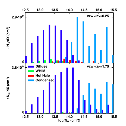
Figure 10: Summed column densities per unit path length as a function of column density, subdivided by absorber phase. The top panel shows absorbers in the range $z=0-0.5$, and the bottom panel shows $z=1.5-2$.

We now examine the cosmic phase of Ly$\alpha$ absorption as a function of column density. Figure 10 shows a sum over H i column density for lines in bins of $N_{\rm HI}$ for our momentum-driven wind model. At both low ($\bar{z}=0.25$) and high ($\bar{z}=1.75$) redshifts, there is a clear transition in which total H i absorption is dominated by diffuse absorbers at low $N_{\rm HI}$ and by condensed absorbers at high $N_{\rm HI}$. The transition occurs at $N_{\rm HI}\approx 10^{14}{\rm cm}^{-2}$ for $\bar{z}=0.25$ and $\approx 10^{14.5}{\rm cm}^{-2}$ for $\bar{z}=1.75$. WHIM and hot halo absorbers are sub-dominant at all column densities, though they are much more common at $\bar{z}=0.25$ than at $\bar{z}=1.75$. While the column density demarcation is less clear for these phases than for diffuse/condensed, WHIM absorbers typically have $N_{\rm HI}<10^{14}{\rm cm}^{-2}$, while hot halo absorbers sometimes have larger $N_{\rm HI}$.

While the broad trends are similar for other wind models, in detail there are substantial differences particularly for absorption in bound phases. If we consider absorbers from $10^{14}\la N_{\rm HI}\la 10^{15.5}{\rm cm}^{-2}$ at $z=0-0.5$, then the cw model contains only half the absorption, and nw only $\approx 40\%$ of the absorption, relative to vzw. This reiterates the result in Figure 6 that high-$N_{\rm HI}$ absorbers provide the most sensitive probe of galactic outflows in the Ly$\alpha$ forest.

In summary, the low-$z$ Ly$\alpha$ forest contains absorbers from all cosmic phases, but diffuse absorbers dominate at $N_{\rm HI}\la 10^{14}{\rm cm}^{-2}$ and condensed absorbers dominate at higher $N_{\rm HI}$. WHIM and hot phase absorbers are present, but highly subdominant in total absorption. Next, we assess whether linewidths add enough information to pinpoint the absorbers arising in WHIM and hot halo gas.

5.4 Linewidths and temperatures

In the absence of other sources of line broadening, the $b$-parameters will reflect the temperature of the underlying absorbing gas. A particularly promising application of this is tracing the missing baryons with wide Ly$\alpha$ lines because, unlike relying on high-ionization metal lines such as O vi (e.g. Tripp, Savage, & Jenkins, 2000) or O vii (e.g. Nicastro et al., 2005), H i linewidths are independent of metallicity. However, in practice, linewidths are not dominated by thermal broadening (Weinberg et al., 1997c), although the thermal contribution is higher at low-$z$ (Davé & Tripp, 2001). Here we investigate the relation between linewidths and temperature in our simulations, to better understand how robustly one can trace the WHIM, and hotter IGM gas in general, using wide Ly$\alpha$ lines.

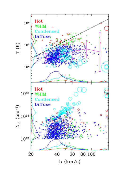
Figure 11: (Top) Temperature vs. $b$-parameter for Ly$\alpha$ absorbers, color-coded by absorber phase, from the vzw simulation at $z=0$. Symbol size is scaled by $\sqrt{N_{\rm HI}/10^{14}}$. Diagonal solid line shows the relation for pure thermal broadening; some absorbers are narrower than “allowed” owing to uncertainties in Voigt profile fitting and the assigning of temperatures to individual absorbers. Histograms in $b$ and $T$ are shown along the bottom and side, respectively, divided by absorber phase, with tick marks above the curves identifying the median values. For visibility of the other phases, the diffuse-phase histograms have been reduced by $5\times$; otherwise, it would dominate at essentially all $b$ values. Magenta curve shows a running median, with $1\sigma$ dispersion, for the entire sample. (Bottom) Like top, but showing H i column density in place of temperature.

Figure 11, top panel, shows the distribution of absorbers’ $b$-parameters versus temperature from our momentum-driven wind simulation at $z\approx 0$ (other wind models are similar). Absorbers are color-coded by cosmic phase as in Figure 4. Recall that we do not fit a continuum to the simulated spectra, hence there is no additional uncertainty in this regard in the identification of broad absorbers in the models. However, such uncertainties may be important when analysing observations, as broad absorbers may be partially “fit out” when fitting a continuum to unnormalized data. There is a definite trend for wider absorbers to arise in hotter gas, as shown by the running median (magenta curve), but there is also substantial scatter as indicated by error bars which show $1\sigma$ dispersion values about the median. Hence, a wide Ly$\alpha$ line is more likely to arise in hotter gas, but it does not always do so.

If lines were purely thermally broadened, then the H i linewidth would be related to the temperature by $b=12.8\sqrt{T/10^{4}{\rm K}}\;{\rm km}\,{\rm s}^{-1}$. This relation is shown as the solid diagonal line. A small fraction of WHIM and hot absorbers are narrower than allowed by thermal broadening, either because of $b$-parameter uncertainties in the Voigt profile fits or because of uncertainties in assigning temperatures to absorbers as described above. Generally, however, most absorbers’ widths significantly exceed the thermal broadening value. The running median shows a similar trend as the thermal broadening track, but it is higher by a factor of $1.5-3$ in $b$, until a turnover at the very largest $b$ values. For the narrow diffuse absorbers, we obtain the same result as in Davé & Tripp (2001) that thermal broadening contributes equally to other sources (in quadrature) in setting the linewidths. For wider absorbers, the thermal contribution becomes smaller. In general, the dominant contribution to the $b$-parameters is not thermal broadening, but rather Hubble broadening in the expanding gas or line blending owing to limited spectral resolution as discussed in §4.4.

Along the bottom and side of Figure 11 are displayed absorber histograms in $b$ and $T$ for each cosmic phase, with the median values indicated by tick marks. The diffuse-phase histogram has been multiplied by $1/5$ along each axis for visibility. The ones along the temperature axis show the expected behavior, with hotter phases having higher median temperatures. The increasing $T$ with $b$ is broadly reflected in the histograms along the $b$-axis as well, with WHIM and hot absobers being at higher $b$ values than diffuse and condensed ones. However, the scatter between $b$ and $T$ is quite significant; the histograms of the various phases span a wide range in $b$ and have a substantial overlap. Moreover, the diffuse absorbers essentially dominate at all $b$ values (remember that this histogram has lowered by $5\times$) simply because they are so numerous, despite the fact that their median linewidth is substantially smaller than all the other phases. Hence, it is unfortunately not straightforward to assign a gas temperature purely from the $b$ parameter. A key implication is that searches for WHIM gas with COS by selecting only broad Ly$\alpha$ lines is likely to pick up a significant fraction of diffuse absorbers, and care must be taken to avoid double-counting baryons in such studies.

Both the column density and linewidth provide some guidance in determining the cosmic phase of the absorbing gas. It stands to reason then that combining the two observables may provide more accuracy in identifying the cosmic phase. The bottom panel of Figure 11 shows the absorbers in $N_{\rm HI}-b$, color-coded by absorber phase. Broad, weak absorbers with $b>60\;{\rm km}\,{\rm s}^{-1}$ and $N_{\rm HI}<10^{14}{\rm cm}^{-2}$ include a relatively large fraction of WHIM absorbers. However, a significant fraction of absorbers in this range are still diffuse, and many WHIM or hot halo absorbers have lower $b$-parameters than this threshold.

In summary, the linewidths trace temperature only fairly loosely, and for any individual absorber it is difficult to pinpoint the cosmic phase purely from observables. Nevertheless, one can assign phases probabilistically based on their location $(N_{\rm HI},b)$, at the penalty of introducing some model dependence. With the large ensembles of absorbers expected to be obtained with COS, this approach can provide some constraints on the content of all baryonic phases as traced by Ly$\alpha$ absorption.

6 Conclusions

We study the low-redshift IGM as traced by Ly$\alpha$ absorbers in $48h^{-1}{\rm Mpc}$, $2\times 384^{3}$-particle cosmological hydrodynamic simulations with three prescriptions for galactic outflows. This work builds on our previous works of a decade ago, namely Davé et al. (1999) and Davé et al. (2001), by employing simulations with $216\times$ more particles and $80\times$ more volume, using improved numerical methodology, and most significantly, testing the impact of large-scale galactic outflows on the IGM as traced by Ly$\alpha$ absorption. Our scenario for the nature and evolution of Ly$\alpha$ forest absorbers from $z=2\rightarrow 0$ remains basically unchanged: most absorbers arise in low-overdensity, highly photoionized gas that traces uncollapsed large-scale filaments. Davé et al. (1999) argued that much of the observed evolution in the Ly$\alpha$ forest can be understood in terms of the evolving relationship between H i column density and the overdensity of the absorbing gas; our latest simulations yield a similar slope and evolution of this relation. Outflows are found to have a small impact on the diffuse IGM, but they do have a significant effect on bound-phase absorbers that arise nearer to galaxies. Our statistical results for Ly$\alpha$ forest absorbers are obtained by applying the AutoVP line-fitter (Davé et al., 1997) to artificial spectra with a resolution and S/N similar to those expected for typical COS observations.

Our main results are as follows:

• Baryons at $z\sim 0$ are divided comparably amongst the diffuse phase, the WHIM, and the bound phases (condensed, hot halo, and stars), The WHIM here is defined as low-density (outside of halos) gas with $T>10^{5}$ K, a notable change from previous definitions that impose a maximum temperature but not a maximum density. In detail, our favoured momentum-driven outflow model has 41% in diffuse gas, 35% in bound phases, and 24% in WHIM at $z=0$, with values for other wind models and redshifts shown in Figure 4.

• Our favoured momentum-driven wind (vzw) model shows similar evolution in diffuse (unbound) IGM baryonic phases to the no-wind (nw) case. In contrast, the condensed, hot halo, and stellar fractions are all noticeably different between those two, and between either of these models and the constant wind (cw) model. Furthermore, cw significantly heats the IGM, resulting in more WHIM and less condensed and diffuse gas.

• The vzw model at COS resolution shows a column density distribution with a power-law slope of $-1.70$. The slope is slightly steeper for nw and cw, and it is steeper for higher-resolution spectra. While formally all slopes are within $\sim 2\sigma$ of each other, recall that the lines of sight are identical through each simulation, so the differences are fairly robust.

• The shallower vzw slope arises because it produces more strong ($N_{\rm HI}>10^{14}{\rm cm}^{-2}$) lines at $z=0$, which agrees better with observations of $dN/dz$ evolution. Weaker lines show no differences in $dN/dz$ among wind models, but they do indicate a discrepancy around $z\sim 1$ that may reflect deviations from the Haardt & Madau (2001) ionizing background evolution.

• The linewidth ($b$) distribution shows a median around $\sim 40\;{\rm km}\,{\rm s}^{-1}$ at COS resolution, and it is insensitive to the wind model. It is highly sensitive to spectral resolution, even at large $b$ values, and much of the broadening owes to instrumental resolution (note that our $b$-parameters are not corrected for this).

• Diffuse Ly$\alpha$ absorbers follow a relation between $N_{\rm HI}$ and overdensity given by $\rho/\bar{\rho}\propto N_{\rm HI}^{0.74}10^{-0.37z}$, in general agreement with our previous findings. This results in a region of a given overdensity giving rise to a lower column density systems at higher redshift. Departures from this relation become more prominent at low-$z$ owing to an increased amount of shock heating.

• The bulk of Ly$\alpha$ absorbers have total hydrogen columns of $\sim 10^{18-19}{\rm cm}^{-2}$, reflecting the trend that the low-$N_{\rm HI}$ absorbers are more ionized (neutral fraction $\sim 10^{-6}$ cm^-3) and larger (hundreds of kpc), while high-$N_{\rm HI}$ absorbers are less ionized (neutral fraction $\sim 10^{-3}$ cm^-3) and smaller (few kpc).

• Linewidths only loosely reflect the temperature of the absorbing gas, because typically linewidths are $1.5-3$ times the thermal broadening value. Hence, wide lines do not exclusively track WHIM or hot gas, though trends in $\rho$ and $T$ with both $b$ and $N_{\rm HI}$ could be used to assign absorbers to a particular cosmic phase in a statistical sense.

• Improved $dN/dz$ statistics for weak lines ($N_{\rm HI}<10^{14}{\rm cm}^{-2}$) will improve determinations of the UV background intensity at $z<2$. Improved statistics at higher column densities can provide strong tests of galactic outflow models.

The installation of COS on Hubble promises a great leap forward in our understanding of low-redshift Ly$\alpha$ absorption and the IGM from which it arises. Besides testing the basic paradigm of the cosmic web origin for weak Ly$\alpha$ forest absorbers, COS Ly$\alpha$ data will provide constraints on the baryon content in various cosmic phases, ionizing background evolution, and the nature of galactic outflows. Additional constraints will be provided by the distribution of IGM metals that can be probed to much greater precision with COS (the subject of Paper II in this series) and by the relation between galaxies and absorption systems (covered in Paper III). The combination of these constraints with overall Ly$\alpha$ absorber statistics will provide powerful diagnostics for the mechanisms of galactic outflows. Comparisons of theory and observations in the coming years will critically test our prevailing paradigms and prescriptions, thereby providing valuable insights into the evolution of the majority of baryons over cosmic time.

References

- Bahcall et al. (1991) Bahcall, J. N., Jannuzi, B. T., Schneider, D. P., Hartig, G. F., Bohlin, R., & Junkkarinen, V. 1991, ApJ, 377, L5
- Bahcall et al. (1996) Bahcall, J. N., et al. 1996, ApJ, 457, 19
- Baldry, Glazebrook, & Driver (2008) Baldry, I. K., Glazebrook, K., Driver, S. P. 2008, MNRAS, 388, 945
- Balogh et al. (2001) Balogh, Michael L., Pearce, Frazer R., Bower, Richard G., Kay, Scott T. 2001, MNRAS, 326, 1228
- Bell et al. (2003) Bell, E. F., McIntosh, D. H., Katz, N., Weinberg, M. D. 2003, ApJ, 585, L117
- Bouwens et al. (2007) Bouwens, R. J., Illingworth, G. D., Franx, M., Ford, H. 2007, ApJ, 670, 928
- Bruzual & Charlot (2003) Bruzual, G. & Charlot, S. 2003, MNRA S, 344, 1000
- Casey et al. (2008) Casey, C. M., Impey, C. D., Petry, C. E., Marble, A. R., Davé, R. 2008, AJ, 136, 131.
- Cen et al. (1994) Cen, R., Miralda-Escudé, J., Ostriker, J.P., & Rauch M. 1994, ApJL, 427, L9
- Cen & Ostriker (1999) Cen, R. & Ostriker, J. P. 1999, ApJ, 514, 1
- Cen & Ostriker (2006) Cen, R. & Ostriker, J. P. 2006, ApJ, 650. 560
- Chabrier (2003) Chabrier, G. 2003, PASP, 115, 763
- Chen et al. (1998) Chen, H.-W., Lanzetta, K. M., Webb, J. K., & Barcons, X. 1998, ApJ, 498, 77
- Croft et al. (1998) Croft, R. A. C., Weinberg, D. H., Katz, N., & Hernquist, L. 1998, ApJ, 495, 44
- Croft et al. (1999) Croft, R. A. C., Weinberg, D. H., Pettini, M., Katz, N., & Hernquist, L. 1999, ApJ, 520, 1
- Croft et al. (2002) Croft, R. A. C., Weinberg, D. H., Bolte, M., Hernquist, L., Katz, N., Kirkman, D., Tytler, D. 2002, ApJ, 581, 20
- Daddi et al. (2007) Daddi, E. et al. 2007, 670, 156
- Dalla Vecchia & Schaye (2008) Dalla Vecchia, C. & Schaye, J. 2008, MNRAS, 387, 1431
- Davé et al. (1997) Davé, R., Hernquist, L., Weinberg, D. H., Katz, N. 1997, ApJ, 477, 21
- Davé et al. (1999) Davé, R., Hernquist, L., Katz, N., Weinberg, D. H. 1999, ApJ, 511, 521
- Davé et al. (2001) Davé, R., Cen, R., Ostriker, J. P., Bryan, G. L., Hernquist, L., Katz, N., Weinberg, D. H., Norman, M. L., & O’Shea, B. 2001, ApJ, 552, 473
- Davé & Tripp (2001) Davé, R., & Tripp, T. M. 2001, ApJ, 553, 528.
- Davé, Finlator & Oppenheimer (2006) Davé, R., Finlator, K., & Oppenheimer, B. D. 2006, MNRAS, 370, 273
- Davé, Finlator, & Oppenheimer (2007) Davé, R., Finlator, K., Oppenheimer, B. D. 2007, in proc. “Chemodynamics 2006: From First Stars to Local Galaxies”, EAS, 24, 183
- Davé, Oppenheimer, & Sivanandam (2008) Davé, R., Oppenheimer, B. D., Sivanandam, S. 2008, MNRAS, 391, 110
- Davé (2008) Davé, R. 2008, MNRAS, 385, 147
- Dinshaw et al. (1998) Dinshaw, N., Foltz, C. B., Impey, C. D., Weymann, R. J. 1998, ApJ, 494, 567
- Eisenstein & Hu (1999) Eisenstein, D. J. & Hu, W. 1999, ApJ, 511, 5
- Eke, Navarro, & Frenk (1998) Eke, V. R., Navarro, J. F., Frenk, C. S. 1998, ApJ, 503, 569
- Erb et al. (2006) Erb, D. K., Shapley, A. E., Pettini, M., Steidel, C. C., Reddy, N. A, & Adelberger, K. L. 2006, ApJ, 644, 813
- Erb (2008) Erb, D. K. 2008, ApJ, 674, 151
- Ferland et al. (1998) Ferland, G., Korista, K. T., Verner, D. A., Ferguson, J. W., Kingdon, J. B., Verner, E. M. 1998, PASP, 110, 761
- Finlator et al. (2006) Finlator, K., Davé, R., Papovich, C., & Hernquist, L. 2006, ApJ, 639, 672
- Finlator & Davé (2008) Finlator, K. & Davé, R. 2008, MNRAS, 385, 2181
- Gingold & Monaghan (1977) Gingold, R.A., & Monaghan, J.J. 1977, MNRAS, 181, 375
- Gunn & Peterson (1965) Gunn, J.E. & Peterson, B.A. 1965, ApJ, 142, 1633
- Haardt & Madau (2001) Haardt, F. & Madau, P. 2001, in proc. XXXVIth Rencontres de Moriond, eds. D.M. Neumann & J.T.T. Van.
- Hernquist et al. (1996) Hernquist, L., Katz, N., Weinberg, D.H., & Miralda-Escudé, J. 1996, ApJL, 457, L51
- Hong et al. (2010) Hong, S., Katz, N., Davé, R., Fardal, M., Keres, D., Oppenheimer, B. D., Weinberg, D. H. 2010, in preparation
- Hui & Gnedin (1997) Hui, L., & Gnedin, N. 1997, MNRAS, 292, 27
- Janknecht et al. (2006) Janknecht, E., Reimers, D., Lopez, S., Tytler, D. 2006, A&A, 458, 427
- Jarosik et al. (2010) Jarosik, N. et al. 2010, ApJS, submitted, arXiv:1001.4744
- Katz et al. (1996) Katz, N., Weinberg, D. H., Hernquist, L. 1996, ApJS, 105, 19
- Kennicutt (1998a) Kennicutt, R. C. 1998a, ApJ, 498, 541
- Kennicutt (1998b) Kennicutt, R. C. 1998b, ARA&A, 36, 189
- Kereš et al. (2005) Kereš, D., Katz, N., Weinberg, D. H., & Davé, R. 2005, MNRAS, 363, 2
- Kereš et al. (2009) Kereš, D., Katz, N., Fardal, M., Davé, R., Weinberg, D. H. 2009, MNRAS, 395, 160
- Kim, Cristiani, & D’Odorico (2001) Kim, T.-S., Cristiani, S., D’Odorico, S. 2001, A&A, 373, 757
- Kirkman et al. (2007) Kirkman, D., Tytler, D., Lubin, D., Charlton, J. 2007, MNRAS, 376, 1227
- Kitayama & Suto (1996) Kitayama, T. & Suto, Y. 1996, ApJ, 469, 480
- Kollmeier et al. (2003) Kollmeier, J. A., Weinberg, D. H., Davé, R., & Katz, N. 2003, ApJ, 594, 75
- Kollmeier et al. (2006) Kollmeier, J. A., Miralda-Escudé, J., Cen, R., & Ostriker, J. P. 2006, ApJ, 638, 52
- Lehner et al. (2007) Lehner, N., Savage, B.D., Richter, P. Sembach, K.R., Tripp, T.M., Wakker, B.P. 2007, ApJ, 658, 680
- Lidz et al. (2009) Lidz, A., Faucher-Giguere, C. -., Dall’Aglio, A., McQuinn, M., Fechner, C., Zaldarriaga, M., Hernquist, L., & Dutta, S. 2009, arXiv:0909.5210
- Limongi & Chieffi (2005) Limongi, M. & Chieffi, A. 2005, ASP conf. ser., v.342, 1604-2004: Supernovae as Cosmological Lighthouses, ASP, San Francisco., p.122
- Lucy (1977) Lucy, L. 1977, AJ, 82, 1013
- Lynds (1971) Lynds, R. 1971, ApJ, 164, L73
- Madau (1998) Madau, P. 1998, in The Hubble Deep Field, eds. M. Livio, S. M. Fall, & P. Madau (Cambridge: Cambridge University Press), p. 200, arXiv:astro-ph/9709147
- McDonald et al. (2000) McDonald, P., Miralda-Escudé, J., Rauch, M., Sargent, W. L. W., Barlow, T. A., Cen, R., & Ostriker, J. P. 2000, ApJ, 543, 1
- McDonald et al. (2006) McDonald, P. et al. 2006, ApJS, 163, 80
- McKee & Ostriker (1977) McKee, C. F. & Ostriker, J. P. 1977, 218, 148
- Miralda-Escudé et al. (1996) Miralda-Escudé, J., Cen, R., Ostriker, J.P., & Rauch, M. 1996, ApJ, 471, 582
- Mo, Mao, & White (1998) Mo, H. J., Mao, S., & White, S. D. M. 1998, MNRAS, 295, 319
- Morris et al. (1991) Morris, S. L., Weymann, R. J., Savage, B. D., & Gilliland, R. L. 1991, ApJ, 377, L21
- Mulchaey (2000) Mulchaey, J. S. 2000, ARA&A, 38, 289
- Murray, Quatert, & Thompson (2005) Murray, N., Quatert, E., & Thompson, T. A. 2005, ApJ, 618, 569
- Navarro, Frenk, & White (1996) Navarro, J. F., Frenk, C. S., White, S. D. M. 1996, ApJ, 490, 493
- Nicastro et al. (2005) Nicastro, F. et al. 2005, Nature, 433, 495
- Oppenheimer & Davé (2006) Oppenheimer, B. D. & Davé, R. 2006, MNRAS, 373, 1265
- Oppenheimer & Davé (2008) Oppenheimer, B. D. & Davé, R. 2008, MNRAS, 387, 577
- Oppenheimer & Davé (2009) Oppenheimer, B. D. & Davé, R. 2009, MNRAS, 395, 1875
- Oppenheimer, Davé, & Finlator (2009) Oppenheimer, B. D., Davé, R., Finlator, K. 2009, MNRAS, 396, 729
- Oppenheimer et al. (2010) Oppenheimer, B. D., Davé, R., Kereš, D., Fardal, M., Katz, N., Kollmeier, J., Weinberg, D. H. 2010, MNRAS, submitted, arXiv:0912.0519
- Paschos et al. (2009) Paschos, P., Jena, T., Tytler, D., Kirkman, D., Norman, M. L. 2009, MNRAS, 399, 1934
- Peeples et al. (2010) Peeples, M. S., Weinberg, D. H., Davé, R., Fardal, M. A., & Katz, N. 2010, MNRAS, 349
- Penton, Stocke, & Shull (2004) Penton, S. V., Stocke, J. T., Shull, J. M. 2004, ApJS, 152, 29
- Prochaska et al. (2004) Prochaska, J. X., Chen, H.-W., Howk, J. C., Weiner, B. J., Mulchaey, J. 2004, ApJ, 617, 718
- Rauch et al. (1997) Rauch, M., Miralda-Escudé, J., Sargent, W. L. W., Barlow, T. A., Weinberg, D. H., Hernquist, L., Katz, N., Cen, R., & Ostriker, J. P., 1997, ApJ, 489, 7
- Rupke, Veilleux & Sanders (2005) Rupke, D. S., Veilleux, S., & Sanders, D. B. 2005, ApJS, 160, 115
- Sanders & Mirabel (1996) Sanders, D. B. & Mirabel, I. F. 1996, ARA&A, 34, 749
- Sargent et al. (1980) Sargent, W.L.W., Young, P.J., Boksenberg, A., & Tytler, D. 1980, ApJS, 42, 41
- Scannapieco & Bildsten (2005) Scannapieco, E. & Bildsten, L. 2005 ApJ, 629, L85
- Schaye (2001) Schaye, J. 2001, ApJ, 559, 507
- Schmidt (1959) Schmidt, M. 1959, ApJ, 129, 243
- Scott et al. (2002) Scott, J., Bechtold, J., Morita, M., Dobrzycki, A., Kulkarni, V. P. 2002, ApJ, 571, 665
- Shankar, Weinberg, Miralda-Escudé (2009) Shankar, F., Weinberg, D. H., Miralda-Escudé, J. 2009, ApJ, 690, 20
- Springel & Hernquist (2002) Springel, V., & Hernquist, L. 2002, MNRAS, 333, 649
- Springel & Hernquist (2003) Springel, V. & Hernquist, L. 2003, MNRAS, 339, 289
- Springel & Hernquist (2003b) Springel, V. & Hernquist, L. 2003, MNRAS, 339, 312
- Springel (2005) Springel, V. 2005, MNRAS, 364, 1105
- Steidel et al. (2004) Steidel, C. C., Shapley, A. E., Pettini, M., Adelberger, K. L., Erb, D. K., Reddy, N. A., Hunt, M. P. 2004, ApJ, 604, 534
- Sutherland & Dopita (1993) Sutherland, R. S. & Dopita, M. A. 1993, ApJS, 88, 253
- Theuns, Leonard, & Efstathiou (1998) Theuns, T., Leonard, A., & Efstathiou, G. 1998, MNRAS, 297, L49
- Theuns et al. (2002) Theuns, T., Viel, M., Kay, S., Schaye, J., Carswell, R. F., Tzanavaris, P. 2002, ApJL, 578, L5
- Tornatore et al. (2010) Tornatore, L., Borgani, S., Viel, M., Springel, V. 2010, MNRAS, 402, 1911
- Tripp, Savage, & Jenkins (2000) Tripp, T. M., Savage, B. D., Jenkins, E. B. 2000, ApJ, 534, L1
- Viel, Haehnelt, & Springel (2004) Viel, M., Haehnelt, M. G., & Springel, V. 2004, MNRAS, 354, 684
- Viel et al. (2008) Viel, M., Becker, G. D., Bolton, J. S., Haehnelt, M. G., Rauch, M., & Sargent, W. L. W. 2008, Physical Review Letters, 100, 041304
- Weinberg, Katz, & Hernquist (1997a) Weinberg, D. H., Katz, N., & Hernquist, L. 1997a, in ASP Conference Series 148, Origins, eds. C. E. Woodward, J. M. Shull, & H. Thronson, (ASP: San Francisco), 21, arXiv:astro-ph/9708213
- Weinberg et al. (1997b) Weinberg, D.H., Miralda-Escudé, J., Hernquist, L., & Katz, N., 1997b, ApJ, 490, 564
- Weinberg et al. (1997c) Weinberg, D.H., Hernquist, L., Katz, N., Croft, R. & Miralda-Escude, J. 1997c, in Proc. of the 13th IAP Colloquium, Structure and Evolution of the IGM from QSO Absorption Line Systems, eds. P. Petitjean & S. Charlot, (Paris: Nouvelles Frontières), p. 133, arXiv:astro-ph/9709303
- Weinberg et al. (1998) Weinberg, D. H., et al. 1998, in Evolution of Large Scale Structure: From Recombination to Garching, eds. A.J. Banday, R. K. Sheth, & L. N. Da Costa, (Twin Press: Vledder NL), 346 arXiv:astro-ph/9810142
- Weiner et al. (2009) Weiner, B. J. et al. 2009, ApJ, 692, 187
- Weymann et al. (1998) Weymann, R. J. et al. 1998, ApJ, 506, 1
- Wiersma et al. (2009) Wiersma, R. P. C., Schaye, J., Theuns, T., Dalla Vecchia, C., Tornatore, L. 2009, MNRAS, accepted
- Williger et al. (2010) Williger, G. M. et al. 2010, MNRAS, in press, arXiv:1002.3401
- Wolfe et al. (2005) Wolfe, A. M., Gawiser, E., Prochaska, J. X. 2005, ARA&A, 43, 861
- Zhan et al. (2005) Zhan, H., Davé, R., Eisenstein, D., Katz, N. 2005, MNRAS, 363, 1145
- Zhang, Anninos, & Norman (1995) Zhang, Y., Anninos, P. & Norman, M.L. 1995, ApJL, 453, L57