Dynamics of 2D Monolayer Confined Water in Hydrophobic and Charged Environments

Abstract

Using molecular dynamics simulations we study the dynamics of a water-like TIP5P model of water in hydrophilic and hydrophobic confinement. We find that in case of extreme nanocofinement such that there is only one molecular layer of water between the confinement surface, the dynamics of water remains Arrhenius with a very high activation energy up to high temperatures. In case of polar (hydrophilic) confinement, The intermediate time scale dynamics of water is drastically modified presumably due to the transient coupling of dipoles with the effective electric field due to the surface charges. Specifically, we find that in the presence of the polar surfaces, the dynamics of monolayer water shows anomalous region – namely the lateral mean square displacement displays a distinct superdiffusive intermediate time scale behavior in addition to ballistic and diffusive regimes. We explain these finding by proposing a simple model. Furthermore, we find that confinement and the surface polarity changes the vibrational density of states specifically we see the enhancement of the low frequency collective modes in confinement compared to bulk water. Finally, we find that the length scale of translational-orientational coupling increases with the strength of the polarity of the surface.

I Introduction

Water is the most ubiquitous liquid and hence plays a very important role in different phenomena. The list of such phenomena ranges across as varied disciplines as physics, chemistry, biology, nanofluidics, geology and atmospheric sciences leshouches ; Ball2008 ; Kumar06PRL ; Buldyrev07 ; Michaelides2007 ; Carrasco2009 ; Rasaiah2008 . Water also falls into a class of complex liquids which are known to have anomalous behavior compared to simple liquids FrankBook ; Debenedetti2003 . The anomalous expansion upon decreasing temperature below $4^{o}$ C and increase of specific heat upon decreasing temperature in the supercooled state are some of the examples of anomalies of water. Indeed, the list of the anomalous behaviors is incomplete and seems to be ever growing Stanley07 ; chaplin .

Studies of water confined in carbon nanotubes and between hydrophobic surfaces suggest that the confining surfaces may induce layering in liquid water in extreme nano confinements Zangi2004 ; Koga2003 . Moreover, first order layering transitions are also observed Zangi2004 ; Koga2000 in hydrophobic confinements. Water can also form wide variety of crystalline phases such as monolayer and bilayer structures Koga2000 ; Koga2001 ; Koga2003 ; Zangi2004 ; zangi1 ; zangi2 ; Kumar2005 in nanoconfinements. Apart from distinct structural changes, water also exhibits dynamic changes depending on the nature of the confining substrates. It has been found the dynamics becomes slow near hydrophilic surfaces compared to hydrophobic surfaces, presumably due to the binding of polar oxygens and hydrogens to the polar groups on the hydrophilic substrates. Moreover, the dynamics in confinement may depend on the surface morphology. Specifically, it was found that a liquid in smooth confinements diffuses faster than when the confining surfaces are rough kb1 . Recent studies  Kumar2005 ; Gallo07 ; Brovchenko07 ; Han2008a ; truskett suggest that both thermodynamic and dynamic anomalies of water are strongly affected when water is confined in small nanopores. It is found that when water is confined between hydrophobic surfaces both thermodynamic and dynamic anomalies shift to low temperatures and low pressures Kumar2005 ; Gallo07 . Although the characteristics of hydrogen bond dynamics of water is bulk-like in hydrophobic confinement, the average life-time decreases Han2008b leading to a shift in the regions of anomalous dynamics and thermodynamics in the P-T plane Kumar2005 ; Gallo07 ; Brovchenko07 ; truskett . Moreover, the long time relaxation of hydrogen bonds depend on the effective system dimensionality Han2008b .

One of the many important questions that can be asked from the biological science perspective is – what role, if at all, water plays in biology ? The answer to such questions is probably not very apparent and requires a systematic effort to understand physical behavior of water under various conditions such as – water in and around ion channels, protein-hydration water, water in different solutions etc. Although there has been a large array of works answering some of the questions chandler1 ; protein ; Hummer00 ; Chen05 ; Liu04 ; xuPNAS ; Buldyrev07 ; Hummer03 ; Kumar06PRL ; Brovchenko06 ; Hanasaki06 ; Raviv2001 ; Berne04 ; nicolas1 ; nicolas2 , the behavior of water is far from fully understood.

In this paper, we study the dynamics of a monolayer water confined between both hydrophobic and polar surfaces. In section II, we describe the system and method and discuss the results of positive and negative surface polarity on the dynamics of water in section III. In section IV, we present the results of the orientational dynamics and translational-orientational coupling and finally we conclude with a discussion and summary in section V.

II System and Method

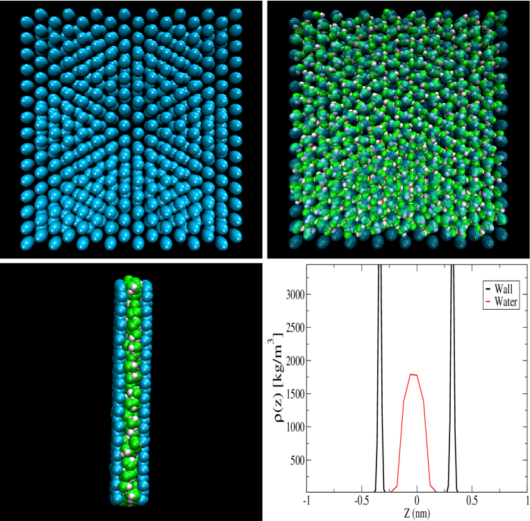
Figure 1: (Color online) Schematics of monolayer water confined between two surfaces. (a) The top view of the confining surfaces. (b) The top view of the confining surface with the water molecules. (c) The lateral view of the confined system. (d) Density profile $\rho(z)$ of the surface atoms and the water molecules along the confinement direction. The effective confinement width due to excluded volume interaction between the water molecules and the surface molecules is $~{}0.320$nm, which is about the diameter of a water molecule.

We perform the molecular dynamics simulation of TIP5P (transferable interaction potential five points) JorgensenXX ; jorgensen2 ; YamadaXX ; Paschek2005 water-like molecules confined between two structured surfaces separated by $0.6$ nm. The separation is chosen such that there is effectively one layer of water between the surfaces (see Fig. 1). The atoms on the surfaces are arranged in a hexagonal packing with $\sigma_{S}=0.339$ nm and do not interact with each other. The positions of the surface atoms were constrained to their respective mean positions by a harmonic potential with spring constant $100$ kJ/mol/nm². In the case of hydrophobic surface, the interaction between the surface atoms and the oxygen of the water molecule is modeled using 6-12 LJ potential U(r)

$$U(r)=4\epsilon[(\frac{\sigma}{r_{SO}})^{12}-\frac{\sigma}{r_{SO}})^{6}]$$ (1)

where $r_{SO}$ is the distance between the surface atom and oxygen of water molecule, and $\sigma=(\sigma_{S}+\sigma_{OW})/2$ and $\epsilon=\sqrt{\epsilon_{S}\epsilon_{OW}}$. $\sigma_{OW}$ and $\epsilon_{OW}$ are the parameters of the LJ interaction between oxygens of water molecules JorgensenXX ; jorgensen2 . The hydrophilicity of the surface is achieved by adding point charge $Qe$ Coulomb to each surface atom and in that case long-range Coulombic interactions between surface atoms and water molecules are added in addition to the LJ interaction. We performed simulations of hydrophobic and hydrophilic confined water in NVT ensemble with the effective density of water $\rho=1.00$ g/cm³. The equations of motion are integrated with a time step of $0.001$ ps and Berendsen’s thermostat is used to attain constant temperature.

III Translational Dynamics and Vibrational Density of States

The translational dynamics in the confined systems can be described by lateral mean-square displacement (MSD) $\langle r_{||}^{2}(t)\rangle$, parallel to surface in the periodic directions. In 2-dimension, the diffusion constant $D_{||}$ can be calculated by using a modified Einstein relation between the long time behavior of the $\langle r_{||}^{2}(t)\rangle$ and $D_{||}$ hansen

$$D_{||}=\lim_{t\rightarrow\infty}\frac{\langle r_{||}^{2}(t)\rangle}{4t}$$ (2)

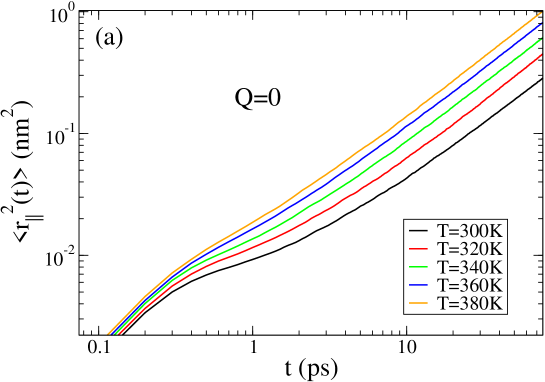
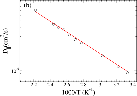
Figure 2: (Color online) (a) $\langle r_{||}^{2}(t)\rangle$ as a function of $t$ for different temperatures when there are no charges on the surface. (b) A linear dependence of $D_{||}$ on $1/T$ on Arrhenius plot shows that the dynamics remains Arrhenius even at high temperatures with an activation energy $E_{A}=14.12$ kJ/mol.

We first study the temperature dependence of $\langle r_{||}^{2}(t)\rangle$ and $D_{||}$ in the case when there are no charges on the surface. In Fig. 2 (a), we show the MSD $\langle r_{||}^{2}(t)\rangle$ for different temperatures. The MSD shows typical time scales –namely a ballistic regime at very small time scales, a cage regime at intermediate time scales, and diffusive regime at long times. In Fig. 2, we show the Arrhenius plot of $D_{||}$ extracted from the long time linear regime of the MSD. We find that the dynamics remains Arrhenius for all the temperature range studied and can be fit with $D_{||}\equiv D_{||}(0)e^{-E_{A}/k_{B}T}$, where $E_{A}=14.12$ kJ/mol and $k_{B}$ are the activation energy and the Boltzmann constant respectively and $D_{||}(0)$ is a fitting parameter. An Arrhenius behavior of $D_{||}$ suggests the the water remains very ordered upto high temperatures in extreme hydrophobic confinements. Moreover, the activation energy is comparable to the low density liquid (where the local structure resembles the IceIh) of bulk water phase.

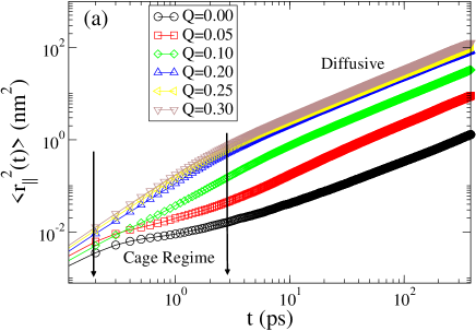
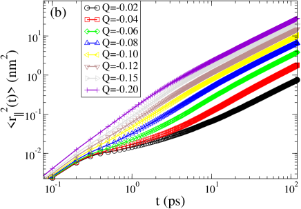
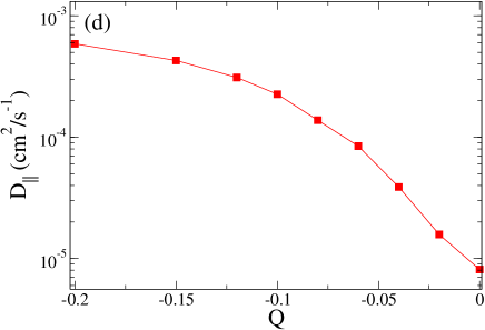
Figure 3: (Color online) (a) Lateral mean square displacement $\langle r_{||}^{2}(t)\rangle$ as a function of $t$ for different values of $Q$. Increasing polarity changes the intermediate time scale dynamics – namely the slope of the cage region increases as the polarity increases. For large values of $Q$, the cage regime becomes superdiffusive. (b) $\langle r_{||}^{2}(t)\rangle$ for the case of surface with negative polarity. The behavior in the case of negative polarity is similar to the case of positive polarity (see Fig. 3 (a)) (c) Lateral diffusion constant $D_{||}$ of water molecules increases with increasing $Q$ and seems to asymptotically saturate to a constant value for large $Q$. (d) Analog of Fig. 3(c) for negative surface polarity.

We next study the translational dynamics in the case when surface atoms have charges on them. In Figure 3(a) and (b), we show the MSD displacement at $T=300$ K as a function $t$ for different strength of surface polarity. For the hydrophobic case when $Q=0$, we find that the dynamics of water in confinement is much slower with a lateral diffusion constant $D_{||}\approx 8.0\rm{x}10^{-6}\rm{cm}^{2}/\rm{s}$. Note that the diffusion constant of TIP5P bulk water at the same density and temperature is $\approx~{}2.5\rm{x}10^{-5}\rm{cm}^{2}/\rm{s}$ YamadaXX . When the polarity of the surface increases, there are namely two changes in the behavior of the MSD – (i) the change in the behavior of cage dynamics or the intermediate time scale dynamics and (ii) increase of the long time MSD and hence the diffusion constant $D_{||}$. In Fig. 3(c) and (d), we show $D_{||}$ for positive and negative polarity of the surfaces respectively. As we would expect the dependence of $D_{||}$ on strength of polarity in both the cases are similar.

Moreover, we find that dynamics in polar confinements is different from dynamics at high $T$ in apolar confinement. A comparison of MSD at high $T$ and $Q=0$ with MSD for $T=300$ and $Q=0.06$ suggests that while at high T and $Q=0$ the MSD changes directly from ballistic to diffusive behavior, the MSD shows a distinct difference at the intermediate time scales in case of polar confining surfaces.

The change in the behavior of the intermediate time scale dynamics can be understood by the fact that although the time average of external electric field at a point inside the confined region is zero, a transient coupling of the fluctuating surface electric field $\vec{E}(\vec{(}x),t)$ with the dipole $\vec{\mu}(\vec{x},t)$ of a water molecule at position $\vec{X}$ will impart a torque $\vec{\mu}(\vec{x},t)X\vec{E}(\vec{x},t)$. The electric field $\vec{E}(\vec{x},t)$ due to one of the surfaces at a position $\vec{x}$ is given by

$$\vec{E}(\vec{x},t)=\frac{1}{4\pi\epsilon}\sum_{i=1}^{N_{q}}Q_{i}\frac{\vec{x}-\vec{x}_{i}}{|\vec{x}-\vec{x}_{i}|^{3}}$$ (3)

where the sum is taken over $N_{q}$ charges on the surface and $\vec{x}_{i}$ are the position vectors of the point charges on the surface. The dynamics of $x_{i}$ follows the dynamics of a Brownian harmonic oscillator and can be written as:

$$\frac{dv_{i}}{dt}=-m\omega^{2}x_{i}-\zeta v_{i}+F(t),$$ (4)

where $F(t)$ is a random force and $\zeta$ is the frictional attenuation due to water. Note that in our system the surface atoms do not interact with each other. Although the set of two equations describes the time dependence of surface electric field, it is almost intractable. To simplify this, we assume that the electric field inside the confined region is due to a flat surface with a fluctuating surface charge density $\sigma(t)$ and hence $\vec{E}(t)$ now will be perpendicular to the surface and can approximately be written as:

$$\vec{E}(t)=\frac{\sigma(t)}{2\epsilon}\hat{z}$$ (5)

where the surface charge density $\sigma(t)$ is

$$\sigma(t)=\frac{N_{q}Q}{A(t)}$$ (6)

where $A(t)$ is the surface area at a given time $t$. Note that the expression for electric field is approximate but we assume that the extent of the surface area considered for $\sigma(t)$ is very large compared to the distance of the point at which we are interested to find the electric field at. Let’s further assume that $A(t)=\bar{A}(1-\frac{\delta A(t)}{\bar{A}})$, we can write the instantaneous fluctuations $\delta\sigma(t)$ in $\sigma$ as:

$$\delta\sigma(t)=\frac{N_{q}Q}{\bar{A}^{2}}\delta A(t),$$ (7)

where $\bar{A}$ is the average area of consideration. Using Eq. 7 we can the time autocorrelation of fluctuations in $\sigma(t)$ as:

$$\langle\delta\sigma(t)\delta\sigma(0)\rangle=\frac{N_{q}^{2}Q^{2}}{\bar{A}^{4}}\langle\delta A(t)\delta A(0)\rangle$$ (8)

Hence the time autocorrelation in the instantaneous fluctuations $\delta E$ of $E$ can be written as:

$$\langle\delta E(t)\delta E(0)\rangle=\frac{N_{q}^{2}Q^{2}}{4\epsilon^{2}\bar{A}^{4}}\langle\delta A(t)\delta A(0)\rangle$$ (9)

Now assuming that $A=Lx.Ly=(x_{n}-x_{1})(y_{n}-y_{1})=xy$, where $x_{1},y_{1}$ and $x_{n},y_{n}$ are the coordinates of the $1^{st}$ and $n^{th}$ point charge along the boundary of the area (note that for simplicity we only cosider the in-plane motion of the point charges). The dynamics of the new coordinates $x$  and $y$ are given by Eq. 4. $\langle\delta E(t)\delta E(0)\rangle$ can now be written as:

$$\langle\delta E(t)\delta E(0)\rangle=\frac{N_{q}^{2}Q^{2}}{2\epsilon^{2}\bar{A}^{3}}\langle\delta x(t)\delta x(0)\rangle=\bar{E}^{2}\frac{2}{\bar{A}}\langle\delta x(t)\delta x(0)\rangle,$$ (10)

where $\delta x=\bar{x}-\delta x(t)$ is the instantaneous fluctuation in $x(t)$ with $\langle\delta x(t)\rangle=0.$For simplification in the above equation, we have assumed $\bar{x}=\bar{y}$. Using Eq. 4 for coordinate $\delta x$, the time autocorrelation of $\delta E$ can be written as:

$$\langle\delta E(t)\delta E(0)\rangle=\bar{E}^{2}\frac{2}{\bar{A}}\frac{k_{B}T}{m\omega_{0}^{2}}e^{-\frac{\zeta}{2m}t}(cos\omega_{1}t+\frac{\gamma}{2m\omega_{1}}sin\omega_{1}t),$$ (11)

where $\omega_{0}=\sqrt{\frac{k}{m}}$ is the characteristic frequency of point charges with spring constant $k$ and mass $m$, and $\omega_{1}=\sqrt{\omega_{0}^{2}-\frac{\zeta^{2}}{4m^{2}}}$. We can write the time autocorrelation of instantaneous fluctuation $\delta E_{T}(t)$ in the net electric field can be written as:

$$\langle\delta E_{T}(t)\delta E_{T}(0)\rangle=\bar{E}^{2}\frac{4}{\bar{A}}\frac{k_{B}T}{m\omega_{0}^{2}}e^{-\frac{\zeta}{2m}t}(cos\omega_{1}t+\frac{\gamma}{2m\omega_{1}}sin\omega_{1}t),$$ (12)

From Eq. 12, we can see that the fast relaxation of autocorrelation of fluctuations in total electric field at a point in the confined region occurs with relaxation time $2m/\zeta$. One would expect that over this time scale the net electric field would not completely vanish in the confined region due to both surfaces and hence there would be a transient coupling of water dipoles with the net electric field. If this energy of dipole coupling is comparable to small frequency collective modes, such transient coupling of dipoles with the surface electric field will lead to a change in the intermediate time scale dynamics. Assuming a surface with uniform charge distribution, a simple estimate shows that $Q=0.10$  would be equivalent to an effective electric field $bar{E}\approx 10^{8}$ V/m. Assuming the length of the considered area to be twice the cut-off length ($\approx$ 2nm), the standard deviation of the net electric field is $\approx 0.22\bar{E}$ at $T=300$ K. In this case, the field-dipole coupling would be large enough to change the low frequency collective vibrations. To verify our picture we calculate the vibrational density of state $D(\omega)$ from the Fourier transform of the velocity autocorrelation function $C(t)$ defined as

$$D(\omega)\equiv\int_{0}^{\infty}C(t)e^{i\omega t}dt,$$ (13)

where $\omega$ is the frequency and $C(t)$ is defined as

$$C(t)\equiv\frac{\langle\vec{v}(t).\vec{v}(0)\rangle}{\langle\vec{v}(0).\vec{v}(0)\rangle}=\frac{1}{Nv(0)^{2}}\sum_{i=1}^{N}\langle\vec{v}_{i}(t).\vec{v}_{i}(0)\rangle.$$ (14)

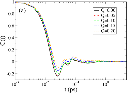
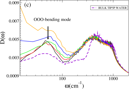
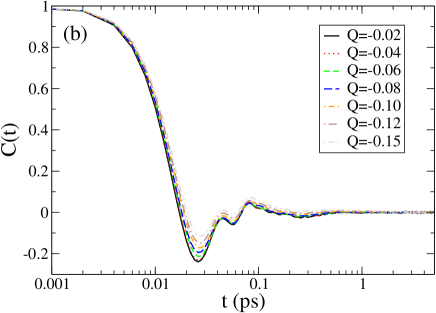
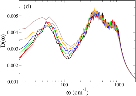
Figure 5: (Color online) (a) Velocity autocorrelation function $C(t)$ as a function of time for different values of the polarity of the surface. The anticorrelation in $C(t)$ begins to disappear as the polarity of the surface increases. (b) Analogue of Fig. 5(a) for negative polarity. (c) Vibrational density of states as calculated from the fourier transform of $C(t)$. A comparison with bulk water $D(\omega)$ shows that the hydrogen bond stretch band ($\approx 210~{}\rm{cm}^{-1}$) is absent in the confinement. Note the merging of diffusive modes into low frequency collective modes when $Q$ increases. (d) Analog of Fig. 5(c) for negative polarity.

where $v_{i}(t)$ denotes the velocity of the $\rm{i}^{\rm{th}}$-water molecule at time $t$ and angular brackets denote the ensemble average. In Fig. 5(a) and (b), we show $C(t)$ for different values of positive and negative polarity of the surface respectively. We find that as the magnitude of the polarity increases, the anticorrelation in $C(t)$ at $t\approx 0.03$ ps decreases. In Fig. 5 (c) and (d), we show the vibrational density of states obtained using equation Eq. 13. A comparison of the bulk TIP5P and confined vibrational density of state shows that the low frequency collective modes are enhanced in confinement. Furthermore, the hydrogen bond stretch mode ($\approx 210$ cm^-1) is absent (or not distinguishable) in the extreme confinement case (see Fig. 5). We find that when magnitude of the polarity increases, the peak corresponding to the OOO bending mode ($\approx 50\rm{cm^{-1}}$) gets broader and merges into the diffusive modes suggesting that highly charged surfaces can modify low frequency collective modes and hence may lead to destruction of the local order.

IV Orientational Dynamics

We next study the orientational dynamics of water molecules since we expect that the transient coupling of fluctuating surface electric field to dipoles of water would provide exteral torque which would tend to align the water dipoles. To study the orientational dynamics of water, we calculated the self-dipole orientational correlation function $C_{d}(t)$ hansen defined as

$$C_{d}(t)=\langle\frac{\vec{\mu}(t).\vec{\mu}(0)}{\vec{\mu}(0).\vec{\mu}(0)}\rangle=\frac{1}{N}\sum\langle\cos\theta_{i}(t)\rangle$$ (15)

where $\vec{\mu}_{i}(t)$ is the dipole of $\rm{i}^{\rm{th}}$ water molecule at time $t$, $\cos\theta_{i}(t)$ is the angle between the dipole vectors of $\rm{i}^{\rm{th}}$-molecule at time $t$ and time $0$.

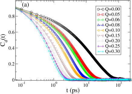
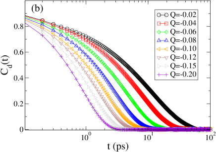
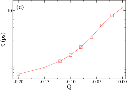
Figure 6: (Color online) (a) Dipole-dipole orientational correlation function $C(t)$ as a function of $t$ for different values of the polarity. C(t) decays faster as the surface polarity is increased. (b) Analog of Fig. 6(a) for negative surface polarity. (c) Orientational correlation time $\tau$ as a function of $Q$ suggests that the orientational correlation time increases monotonically. (d) Analog of Fig. 6(c) for negative surface polarity.

In Fig. 6 (a) and (b), we show $C_{d}(t)$ for different positive and negative values of $Q$. We find that, for small magnitude of $Q$, the orientational correlation function $C_{d}(t)$ decays to zero slowly. To quantify the characteristic time of orientational correlations, we define correlation time $\tau$ as the time at which $C_{d}(t)$ decays by a factor of $e$. In Fig. 6 (c) and (d), we show $\tau$ for the positive and negative surface polarity respectively. We find that, as the magnitude of $Q$ increases, $\tau$ decreases and seems to saturate to a constant value for larger magnitudes of $Q$.

A significant coupling of translational and orientational motion is found in bulk water Chen1997 ; Mazza2006 and other confined systems Joseph2008 . Since we can expect that the presence of the charges of the confining surfaces strongly influence the dipole fluctuations of the confined water, we would also expect that changing the polarity may lead to a change in the effective length scale of the coupling of the translational and orientational dynamics. The characterize the the effective length scale of the coupling between translational and orientational motion, we define $\xi$

$$\xi=\sqrt{\rm{D}_{||}*\tau}$$ (16)

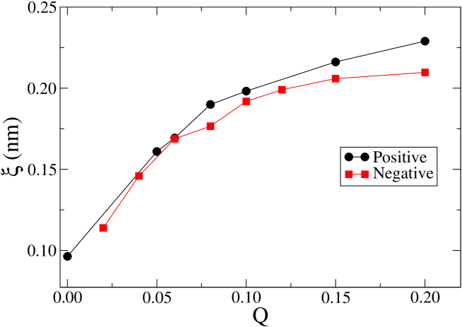
Figure 7: Translation-orientational coupling length scale $\xi$ as a function of atomic charge on the surface. The circles and squares are for positive and negative polarity respectively. $\xi$ increases as the the magniture of the charges increases for both polarities of the surface.

We interpret $\xi$ as the effective length scale over which translational and orientational motions are coupled. Figure  7 shows $\xi$ for different values of $Q$ for both positive and negative $Q$. The value $\xi$ increases as the $Q$ is increased and seems to aysmptotically reach a constant value. Furthermore, we find that the value of $\xi$ is similar for both positive and negative surface polarities.

V Summary and Discussions

In summary, using molecular dynamics simulations of TIP5P model of water, we have investigated the dynamics of a monolayer water system confined between hydrophobic and hydrophilic surfaces of different polarity. We find that dynamics of monolayer water in hydrophobic confinement remains Arrhenius upto very large temperatures with a very high activation energy $E_{A}=14.12$ kJ/mol. Further, we find that the transient coupling of the water dipoles with the electric field of the surface gives rise to distinct cage dynamics. Specifically at high polarity the slope of the MSD as a function of $t$ at the intermediate time scales becomes $>1.0$ on a log-log scale, giving rise to three distinct dynamic regions –ballistic at very small time scales, superdiffusive at intermediate times and a long time diffusive behavior. Note that although the effect of transient coupling of water dipoles to the external field is effective increase of diffusion of the system, the dynamic changes are very different in the two cases. While at high temperatures MSD would only show two distinct regimes, water in polar confinements has a different intermediate time scale dynamics and three distinct regimes. We explain these finding by proposing a simple model of electric field fluctuations in the confined region. We further find that the extreme confinement enhances the low frequency collective modes. Moreover, we find that the presence of a highly polar surface disrupts the low frequency collective vibrational modes and hence leads to less ordered system, suggesting that while extreme hydrophobic confinement increases the order, the presence of a highly polar surface makes the water molecule relatively more disordered in confinement. Finally, we calculated the effective length scale of coupling of translational and orientational motions and find that the coupling length scale increases as the polarity of the surface increases.

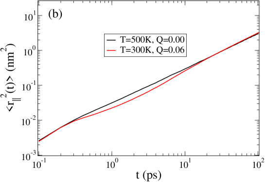
Figure 4: (Color online) (a) Lateral mean square displacement $\langle r_{||}^{2}(t)\rangle$ for $Q=0.20$ showing three distinct regimes in the dynamics – small time ballistic motion, intermediate time superdiffusive, and long time diffusive behaviors. (b) Comparison of MSD at high $T$ and $Q=0$ with MSD for $T=300$ and $Q=0.06$ suggest that while at high $T$ and $Q=0$ the MSD changes from ballistic to diffusive behavior as expected for bulk liquids, the MSD shows a different behavior at the intermediate time scales in the case of polar confining surfaces.

References

- (1) M.-C. Bellissent-Funel, ed., Hydration Processes in Biology: Theoretical and Experimental Approaches [Proc. NATO Advanced Study Institutes, Vol. 305] (IOS Press, Amsterdam, 1999).
- (2) P. Ball, Chem. Rev. 108 (1), 74 (2008).
- (3) P. Kumar, Z. Yan, L. Xu, M. G. Mazza, S. V. Buldyrev, S.-H. Chen, S. Sastry, and H. E. Stanley, Phys. Rev. Lett. 97, 177802 (2006).
- (4) S. V. Buldyrev, P. Kumar, P. G. Debenedetti, P. Rossky, and H. E. Stanley, Proc. Nat. Acad. Sci. USA 104, 20177 (2007).
- (5) A. Michaelides, and Karina Morgenstern, Nature Materials 6, 597 (2007).
- (6) J. Carrasco, A. Michaelides, M. Forster, S. Haq, R. Raval, and A. Hodgson, Nature Materials 8, 427 (2009).
- (7) J. C. Rasaiah, S. Garde, and Gerhard Hummer, Annu. Rev. Phys. Chem. 59, 713 (2008).
- (8) Water: A Comprehensive Treatise, Vol. 1. The Physics and Physical Chemistry of Water Editor: F. Frank, Plenum Press, New York (1972) .
- (9) P. G. Debenedetti and H. E. Stanley, Physics Today 56 (6), 40 (2003).
- (10) H. E. Stanley et. al. Physica A 386, 729 (2007).
- (11) http://www.lsbu.ac.uk/water/.
- (12) R. Zangi, J. Phys.: Condens. Mat. 16, S5371 (2004).
- (13) K. Koga, J. Chem. Phys. 118, 7973 (2003).
- (14) K. Koga, H. Tanaka, and X. C. Zeng, Nature 408, 564 (2000).
- (15) K. Koga, G. T. Gao, H. Tanaka, and X. C. Zeng, Nature 412, 802 (2001).
- (16) R. Zangi and A. E. Mark, Phys. Rev. Lett. 91, 0255502 (2003).
- (17) R. Zangi and A. E. Mark, J. Chem. Phys. 120, 7123 (2004).
- (18) P. Kumar, S. V. Buldyrev, F. W. Starr, H. E. Stanley Phys. Rev. E 72, 051503 (2005).
- (19) P. Scheidler, W. Kob, and K. Binder, Europhys. Lett. 59, 701 (2002).
- (20) D Corradini, P Gallo, and M Rovere, J. Chem. Phys. 128, 244508 (2008).
- (21) I. Brovchenko and A. Oleinikova, J. Chem. Phys. 126, 214701 (2007).
- (22) S. Han, P. Kumar, and H. E. Stanley, Phys. Rev. E 77, 030201(R) (2008).
- (23) T. M. Truskett and P. G. Debenedetti, J. Chem. Phys. 114, 2401 (2001).
- (24) S. Han, P. Kumar, and H. E. Stanley, Phys. Rev. E 79, 041202 (2009).
- (25) K. Lum, D. Chandler, and J. D. Weeks, J. Phys. Chem. B 103, 4590 (1999).
- (26) R. Zhou, B. J. Berne, and R. Germain, Proc. Nat. Acad. Sci. 98, 14931 (2001); M. Tarek and D. J. Tobias, Phys. Rev. Lett. 89, 275501 (2002).
- (27) G. Hummer, S. Garde, A. E. Garcia, and L. R. Pratt, Chemical Physics 258, 349 (2000).
- (28) S.-H. Chen, L. Liu, E. Fratini, P. Baglioni, A. Faraone, and E. Mamontov, Proc. Nat. Acad.Sci. USA 103, 9012 (2006).
- (29) L. Liu et al., Phys. Rev. Lett. 95, 117802 (2005).
- (30) L. Xu et al., Proc. Natl. Acad. Sci. USA 102, 16558 (2005).
- (31) A. Kalra, S. Garde, and G. Hummer, Proc. Natl. Acad. Sci. USA. 100, 10175 (2003).
- (32) I. Brovchenko, A. Krukau, and A. Oleinikova, Phys. Rev. Lett. 97, 137801 (2006).
- (33) I. Hanasaki and A. Nakatani, J. Chem. Phys. 124, 174714 (2006).
- (34) U. Raviv, P. Laurat, and J. Klein, Nature 413, 51 (2001).
- (35) P. Liu, E. Harder, and B. J. Berne, J. Phys. Chem. B 108, 6595 (2004).
- (36) N. Giovambattista, P.J. Rossky and P.G. Debenedetti, Phys. Rev. Lett. 102, 050603 (2009).
- (37) N. Giovambattista, P.G. Debenedetti and P.J. Rossky, J. Phys. Chem. C 111, 1323 (2007).
- (38) M. W. Mahoney and W. L. Jorgensen, J. Chem. Phys. 112, 8910 (2000).
- (39) M. W. Mahoney and W. L. Jorgensen, J. Chem. Phys. 114, 363 (2001).
- (40) M. Yamada et al., Phys. Rev. Lett. 88, 195701 (2002).
- (41) D. Paschek, Phys. Rev. Lett. 94, 217802 (2005).
- (42) J. P. Hansen and I. R. McDonald, Theory of Simple Liquids, (Academic Press, London, 1996).
- (43) S.-H. Chen, P. Gallo, F. Sciortino, and P. Tartaglia, Phys. Rev. E. 56, 4231 (1997).
- (44) M. Mazza, N. Giovambattista, Francis W. Starr, and H. E. Stanley, Phys. Rev. Lett. 96 057803 (2006).
- (45) S. Joseph and N. R. Aluru, Phys. Rev. Lett. 101 064502 (2008).