Stochastic amplification in an epidemic model with seasonal forcing

Abstract

We study the stochastic susceptible-infected-recovered (SIR) model with time-dependent forcing using analytic techniques which allow us to disentangle the interaction of stochasticity and external forcing. The model is formulated as a continuous time Markov process, which is decomposed into a deterministic dynamics together with stochastic corrections, by using an expansion in inverse system size. The forcing induces a limit cycle in the deterministic dynamics, and a complete analysis of the fluctuations about this time-dependent solution is given. This analysis is applied when the limit cycle is annual, and after a period-doubling when it is biennial. The comprehensive nature of our approach allows us to give a coherent picture of the dynamics which unifies past work, but which also provides a systematic method for predicting the periods of oscillations seen in whooping cough and measles epidemics.

1 Introduction

The availability of extensive time-series data for childhood diseases is often the reason given for the amount of attention that this subject receives. However, the possibility that relatively simple models can capture the essence of the disease dynamics also makes the topic an attractive one for modellers. Mathematical epidemiologists are especially intrigued by the rich variety of oscillatory dynamics seen in this data (Earn et al., 2000; Grenfell et al., 2002). Within the literature there is a broad consensus that there are two main elements needed to model these oscillations: firstly stochasticity, due to the individual nature of the population (Bartlett, 1960; Durrett and Levin, 1994); and secondly, seasonal forcing, arising from the term-time aggregation of children in schools, which is deterministic (London and York, 1973; Schenzle, 1984; Altizer et al., 2006). Independently these two factors are well understood, but how they interact when both included in the same model is still an open question (Keeling et al., 2001; Rohani et al., 2002; Coulson et al., 2004).

Measles is the canonical example of a disease which displays recurrent epidemic behaviour. In larger cities regular periodic oscillations, usually annual or biennial, are observed, whereas smaller cities display more irregular dynamics (Grenfell et al., 2002; Lloyd and Sattenspiel, 2009). The introduction of mass vaccination in the 1960s provides a ‘natural experiment’ after which the dynamics become much more irregular (Grenfell and Harwood, 1997). One of the early successes in the field was a simple deterministic model with seasonal forcing which could recreate the regular dynamics of measles (Dietz, 1976; Schwartz and Smith, 1983). Where simple models such as this fail, is in capturing the more irregular dynamics seen in smaller populations (Grenfell et al., 2002), after vaccination (Rohani et al., 1999), and in other diseases such as whooping cough (Nguyen and Rohani, 2008). These aspects can only be captured by fully stochastic models.

Stochastic models without external forcing show large oscillations caused by the stochasticity exciting the system’s natural frequency (Bartlett, 1957; Alonso et al., 2007). When forcing is included, it is less clear how the stochasticity interacts with the cyclic solutions that are produced. It could act passively to kick the system between different deterministic states (Schwartz, 1985), as well as interacting with the non-linearity to excite the transients. Power spectra (Priestley, 1982; Anderson et al., 1984) have proved a useful tool in investigating these factors. They can help distinguish various components in the time-series and classify them as essentially seasonal, stochastic or an interaction of the two (Benton, 2006). The most successful synthesis, by Bauch and Earn (2003b), showed that a simple mechanistic model can accurately predict the position of peaks in the power spectrum of a number of different disease time series.

We approach this problem by starting with an individual based model, which is inherently stochastic. We can then both simulate it and derive the emergent population level dynamics. The novel aspect of this work is that we calculate the power spectrum analytically for explicitly time-dependent external forcing, and compare the results with stochastic simulations. We do this by formulating the model as a master equation which can then be studied using van Kampen’s (1992) expansion in the inverse system size. The macroscopic dynamics can then be viewed as a sum of a deterministic and a stochastic part. The value of the analytic approach is that we can more easily deduce the mechanisms behind the dynamics and better understand the interplay between deterministic and stochastic forces.

The theory we develop in this paper unifies much of the previous work on these models. It encompasses the influential work of Earn et al. (2000) in understanding the transitions in measles epidemics, the later work of Bauch and Earn (2003b) relating to the transient fluctuations close to cyclic attractors for different diseases and the more recent work on stochastic amplification in epidemic models (Alonso et al., 2007; Black and McKane, 2010). The picture that emerges is close to that proposed by Bauch and Earn (2003b), but goes beyond it in two important respects. Firstly, we calculate the exact power spectrum for the forced model. Secondly, we show how the forcing changes the form of the fluctuations, and how in a stochastic model these are intimately related to the period doubling bifurcation, which is vital for explaining the dynamics of measles.

The rest of this paper is as follows. In section 2 we introduce the seasonally-forced version of the stochastic susceptible-infected-recovered (SIR) model and the system-size expansion of the master equation. Section 3 provides a discussion of the results for the simple case when the deterministic dynamics are described by an annual limit cycle. In Section 4 we apply our method to elucidate the dynamics investigated by Earn et al. (2000), which can account for the transitions in measles epidemics. This is an interesting parameter regime, as the deterministic theory predicts a period doubling bifurcation. Finally, in section 5 a broad discussion of our results is given, describing how this approach can account for the different dynamics of measles and whooping cough. There are two appendices giving technical details relating to the system-size expansion and Floquet theory.

2 The seasonally forced SIR model

We first summarise the individual-based stochastic SIR model. We emphasise only the aspects which are relevant to this paper; a more general discussion can be found in textbooks on the subject (Anderson and May, 1991; Keeling and Rohani, 2007). The population is split into three classes: susceptibles, infected and recovered. Birth and death rates are set equal to $\mu$ and these events are linked, even in the stochastic model, so that the total population, $N$, remains constant. Recovery happens at a constant rate $\gamma$, so that the average infectious time is $1/\gamma$; once recovered, an individual is immune for life. Seasonal forcing is included by assuming that the transmission rate $\beta(t)$ follows a term-time pattern (Schenzle, 1984),

$$\beta(t)=\beta_{0}(1+\beta_{1}\text{term}(t)),$$ (1)

where $\beta_{0}$ is the baseline contact rate, $\beta_{1}$ the magnitude of forcing and $\text{term}(t)$ is a periodic function which switches between $1$ during school terms and $-1$ during holidays. In this paper we use the England and Wales term dates set down by Keeling et al. (2001). The reproductive ratio is determined by $R_{0}=\langle\beta\rangle/\gamma$, where $\langle\beta\rangle$ is the effective (time-averaged) transmission rate:

$$\langle\beta\rangle=\beta_{0}[p_{s}(1+\beta_{1})+(1-p_{s})(1-\beta_{1})],$$ (2)

and $p_{s}$ is the proportion of time spent in school. For our choice of terms $p_{s}=0.75$. We also include a small immigration term, $\eta$, to account for infectious imports. We use a commuter formulation, where susceptibles are in contact with a pool of infectives outside the main population (Engbert and Drepper, 1994; Alonso et al., 2007). Since $N=S+I+R$, we can use this constraint to eliminate the variable $R$ from the rate equations.

The model is then defined by the processes through which it evolves. If we write the state of the system as $\sigma\equiv\{S,I\}$, we can specify the following transition rates, $T(\sigma|\sigma^{\prime})$, between an initial state $\sigma^{\prime}$ and a final state $\sigma$:

1. Infection: $S+I\xrightarrow{\beta(t)}I+I$ and $S\xrightarrow{\eta}I$.

   $$T(S-1,I+1|S,I)=\Bigl{(}\beta(t)\frac{S}{N}I+\eta S\Bigr{)}.$$ (3)

2. Recovery: $I\xrightarrow{\gamma}R$.

   $$T(S,I-1|S,I)=\gamma I.$$ (4)

3. Death of an infected individual: $I\xrightarrow{\mu}S$.

   $$T(S+1,I-1|S,I)=\mu I.$$ (5)

4. Death of a recovered individual: $R\xrightarrow{\mu}S$.

   $$T(S+1,I|S,I)=\mu(N-S-I).$$ (6)

Since birth and death are coupled, the processes 3 and 4 also imply the birth of a susceptible individual. An important point is that changes in vaccination can be mapped onto the effective transmission rate $\langle\beta\rangle$ using (Earn et al., 2000)

$$\langle\beta\rangle\rightarrow\langle\beta\rangle(1-p),$$ (7)

where $p$ is the proportion of individuals vaccinated at birth. We can also approximately map a change in birth rates onto $\langle\beta\rangle$, but this is not exact in this model because births and deaths are linked. In this paper we are primarily interested in the parameter range of childhood diseases. These are characterised by $\mu\ll\gamma$, i.e. the average life expectancy of an individual is orders of magnitude longer than the mean infectious period (Anderson and May, 1991).

2.1 Methods of analysis

We use two methods to investigate the dynamics of this system. Firstly we simulate the system using Gillespie’s (1976) algorithm with the appropriate time-dependent extensions (Anderson, 2007). This method generates exact realisations from which statistical quantities, such as power spectra and moments, can be computed. The second method is analytic, through the construction of a master equation. The master equation describes the evolution of the probability distribution of finding the system in state $\sigma$ at time $t$,

$$\frac{dP(\sigma;t)}{dt}=\sum_{\sigma^{\prime}\neq\sigma}T(\sigma|\sigma^{\prime})P(\sigma^{\prime};t)-\sum_{\sigma^{\prime}\neq\sigma}T(\sigma^{\prime}|\sigma)P(\sigma;t).$$ (8)

This cannot be solved exactly so we instead use van Kampen’s (1992) expansion in the inverse system size to derive approximate analytic solutions. This involves making the substitutions,

$$S=N\phi+N^{1/2}x,$$ (9)

$$I=N\psi+N^{1/2}y,$$

and expanding the master equation in powers of $N^{-1/2}$. This technique and similar ones have been documented at length in the literature, but almost exclusively for time-independent models (Alonso et al., 2007). The novel aspect of this paper is that we analyse the full time-dependent system (Boland et al., 2009), whereas in a previous paper we used the approximation which replaced $\beta(t)$ by $\langle\beta\rangle$ (Black and McKane, 2010).

The details of the system-size expansion for this model are given in Appendix A. At leading order we find a pair of deterministic equations, describing the mean behaviour, which scale with the system size $N$,

$$\dot{\phi}=-\beta(t)\phi\psi-\eta\phi+\mu(1-\phi),$$ (10)

$$\dot{\psi}=\beta(t)\phi\psi+\eta\phi-(\mu+\gamma)\psi.$$

These are the same as the equations that are found from a purely phenomenological treatment of the SIR system. At next-to-leading order we obtain a pair of Langevin equations for the stochastic corrections to the deterministic equations (10),

$$\dot{\mathbf{x}}=K(t)\mathbf{x}(t)+\mathbf{f}(t),$$ (11)

where $\mathbf{x}\equiv\{x,y\}$, and $\mathbf{f}(t)$ are Gaussian white-noise terms with correlation function $\langle\mathbf{f}(t)\mathbf{f}(t^{\prime})^{T}\rangle=G(t)\delta(t-t^{\prime})$. The matrices $K(t)$ and $G(t)$ are determined from carrying out the expansion and are given by

$$K(t)=\begin{pmatrix}-\beta\bar{\psi}-\eta-\mu&-\beta\bar{\phi}\\ \beta\bar{\psi}+\eta&\beta\bar{\phi}-\gamma-\mu\end{pmatrix},$$ (12)

and

$$G_{11} =\beta\bar{\phi}\bar{\psi}+\eta\bar{\phi}+\mu(1-\bar{\phi}),$$ (13)

$$G_{22} =\beta\bar{\phi}\bar{\psi}+\eta\bar{\phi}+(\gamma+\mu)\bar{\psi},$$

$$G_{12}=G_{21} =-\beta\bar{\phi}\bar{\psi}-\eta\bar{\phi}-\mu\bar{\psi},$$

where a bar indicates that the solutions are evaluated on the limit cycle. These are essentially the same as are found in the non-forced model (Alonso et al., 2007), except now $\beta$, $\bar{\phi}$ and $\bar{\psi}$ are all functions of time.

3 Stochastic amplification about a limit cycle

The mean behaviour is found by integrating the deterministic equations (10). When $\beta_{1}=0$, solutions show damped oscillations tending to a fixed point (Anderson and May, 1991). For non-zero $\beta_{1}$, this model can display a rich set of dynamics including chaos (Olsen et al., 1988; Rand and Wilson, 1991), but for realistic parameter values the most common long-time solution is a limit cycle with a period that is an integer multiple, $n$, of a year (Dietz, 1976; Schwartz and Smith, 1983). As the forcing is a step function in time, we can visualise this as the system alternately switching between two spiral fixed-points (Keeling et al., 2001) resulting in a piecewise continuous limit cycle, illustrated in figure 1. Any other periodic forcing function, for instance a sinusoidally varying one, could be used without more difficulty, and would typically lead to a limit cycle which is smooth. As $\beta_{1}$ is increased, the limit cycle grows (although typically not linearly with $\beta_{1}$) and at critical values bifurcations are induced to longer period solutions (Aron and Schwartz, 1984; Kuznetsov and Piccardi, 1994).

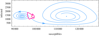
Figure 1: Phase portrait illustrating a deterministic solution of the forced SIR model. The term-time forcing creates a limit cycle (red curve) as the system alternately spirals between the two fixed points defined by $\beta_{H}=\beta_{0}(1+\beta_{1})$ and $\beta_{L}=\beta_{0}(1-\beta_{1})$. The light blue solutions show the behaviour if the forcing was switched off, to illustrate the two spiral attractors. The red dot shows the fixed point calculated using the approximation where $\beta(t)$ is replaced by $\langle\beta\rangle$.

In this section we present results where there is only an annual limit-cycle ($n=1$). The case where we also have a period doubling is examined in section 4. The stability of these limit-cycle solutions can be investigated with the use of Floquet theory (Kuznetsov, 2004; Boland et al., 2009). This quantifies how perturbations to the trajectory of the limit cycle behave and is analogous to linear stability analysis about a fixed point (Grimshaw, 1990).

Floquet theory states that for any periodic solution of Eq. (10) there exists a matrix $B$ which satisfies the relation,

$$X(t+T_{n})=X(t)B,$$ (14)

where $X(t)$ is the fundamental matrix (Grimshaw, 1990) and $T_{n}$ is the period of the limit cycle. The eigenvalues of $B$ are called the Floquet multipliers, $\rho_{i}$; a related set of quantities are the Floquet exponents $\lambda_{i}=\ln(\rho_{i})/T_{n}$ (in this paper, since we will be discussing frequencies rather than angular frequencies, these exponents will be divided by a factor of $2\pi$). Another way to think of this is as linear stability analysis of the fixed points of the $n$-cycle Poincare map of the system (Bauch and Earn, 2003b; Kuznetsov, 2004). A limit-cycle solution will be stable if $|\rho_{i}|<1$. When the multipliers are complex, perturbations to the trajectories return to the limit-cycle in a damped oscillatory manner, analogous to a stable spiral fixed point (Grimshaw, 1990). Similar ideas have been used to investigate the transients in forced epidemic systems in the past, but only in a deterministic setting (Bauch and Earn, 2003b; He and Earn, 2007). Here we will explore how the nature of the fluctuations can be quantified using Floquet theory.

Figure 2: Phase portrait of the stochastic SIR system. A time-series of 100 years duration is shown in light blue. The first two years are highlighted in dark blue, with the dot showing the start point. The macroscopic limit-cycle (red) is also superimposed. Parameters are those relevant for whooping cough (Nguyen and Rohani, 2008): $R_{0}=17$, $\gamma=1/22$, $\beta_{1}=0.25$, $\mu=5.5\times 10^{-5}$, $\eta=10^{-6}$ and $N=2\times 10^{6}$.

Figure 2 shows a simulation of the full stochastic system together with the deterministic limit-cycle solution. We can see that even for large populations the stochastic corrections to the deterministic solution are important. The noise due to demographic stochasticity (noise at the individual level due to chance events; Nisbet and Gurney 1982) excites the natural oscillatory modes about the limit cycle, creating a resonance and giving rise to large scale coherent oscillations—an effect known as stochastic amplification (McKane and Newman, 2005; Alonso et al., 2007). As described in Appendix B, by solving Eq. (11), and invoking aspects of Floquet theory, we can express the auto-correlation function,

$$C(\tau)=\frac{1}{T_{n}}\int_{0}^{T_{n}}\langle\mathbf{x}(t+\tau)\mathbf{x}^{T}(t)\rangle\,dt,\ \ \mathbf{x}\equiv\{x,y\},$$ (15)

as an integral without further approximation (Boland et al., 2009). Taking the Fourier transform of this expression then gives an exact expression for power spectrum of these stochastic oscillations.

Figure 3 shows simulated and analytic power spectra for the system shown in figure 2. We observe a sharp peak at 1 year due to the deterministic annual limit-cycle and a number of broader peaks due to the stochastic amplification of the transients. We would expect on general grounds that the stochastic peaks would be observed at frequencies,

$$m/T_{n}\pm{\rm Im}(\lambda),$$ (16)

where $m$ is an integer and $\lambda$ is the Floquet exponent (Wisenfeld, 1985b; Boland et al., 2009), and this is indeed what is seen. For the annual limit-cycle the dominant peak is at $0+\text{Im}(\lambda)$, with the other peaks being much smaller. Near to bifurcations these minor peaks become important and are treated in more detail in the following section.

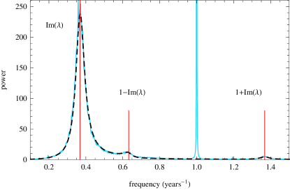
Figure 3: Power spectra for the number of infectives from simulation (light blue solid curve) and analytic calculation (black dashed curve). From the simulations, we observe a sharp peak at 1 year from the deterministic annual-limit cycle. The other peaks, marked by the red lines, are from stochastic amplification, with the peak frequencies given by $m\pm\text{Im}(\lambda)$, where $\text{Im}(\lambda)=0.36$. The dominant stochastic period is therefore $1/0.36=2.7$ years. Parameters are as in figure 2

The area under the peaks in the power spectrum is proportional to the root-mean-square amplitude of the oscillations. Away from any deterministic bifurcation points the amplitude is proportional to Re$(\lambda)$, as in the unforced model. Thus the spectrum is close in form to that predicted from the unforced model by substituting $\langle\beta\rangle$ for the time-independent transmission rate (Bauch and Earn, 2003a; Black and McKane, 2010).

There is good agreement between analytical calculations and simulations. Although calculations give the power spectrum as an integral, it must be evaluated numerically because the deterministic equations (10) cannot be solved in closed form; this is all carried out using the symbolic package Mathematica (Wolfram Research, 2008). This analysis about an annual limit cycle corresponds to that of Bauch and Earn (2003b) except that we can derive the full power spectrum. They term the ‘resonant peak’ what we describe as the deterministic or annual peak, and the ‘non-resonant peak’ what we describe as the stochastic peaks. Their terminology is somewhat misleading, as the stochastic peak is generated by a resonance phenomena whereas the macroscopic peak is not.

4 Period doubling and measles transitions

We can use our analytic methods to help understand the dynamics and large-scale temporal transitions in measles epidemic patterns, first investigated by Earn et al. (2000). The main force in driving these transitions is changes in the susceptible recruitment (a mixture of changes in birth rates and vaccination), which can be mapped onto $R_{0}$. Thus a knowledge of the model dynamics as a function of $R_{0}$ can be used to explain the changes in epidemic patterns. Although the analysis of Earn et al. (2000) is in good qualitative agreement with time-series data, there are a number of outstanding questions with regard to the interpretation of the mechanisms for the dynamics. We first provide a brief review of the original analysis and then go on to show how the stochastic dynamics of this model can be understood within the framework we have laid out in the previous section.

4.1 Review of original analysis

It is acknowledged that stochasticity plays a role in the dynamics of measles, which can only be captured through simulation of the individual-based model. Fundamentally though, the analysis of these mechanisms by Earn et al. (2000) is deterministic. Figure 4 shows the bifurcation diagram derived from the SIR equations (10), as a function of $R_{0}$, with parameters corresponding to measles and no immigration ($\eta=0$). This shows the incidence sampled annually on the 1st of January each year, thus stable limit cycles are shown by different numbers of (colour coded) curves. The single curve, beginning at small $R_{0}$, shows an annual cycle which bifurcates at $R_{0}=15.5$ into two curves giving a biennial cycle. For values of $R_{0}$ lying between about 5 and 15, there are several sets of $n$ curves representing $n$-year cycles.

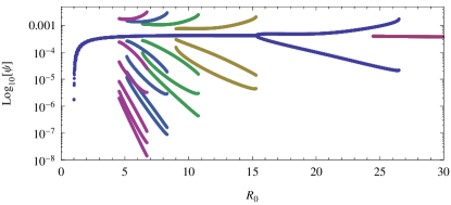
Figure 4: Bifurcation diagram showing the SIR dynamics as a function of $R_{0}$. Fixed parameters: $\beta_{1}=0.29$, $\gamma=1/13$, $\mu=5.5\times 10^{-5}$ and $\eta=0$. The different period limit cycles are shown in different colours, which are produced by different initial conditions.

For large $R_{0}$ (e.g. $R_{0}\approx 30$) only an annual limit cycle exists. As $R_{0}$ is reduced a biennial limit-cycle is found; before vaccination was introduced in England and Wales, most cities would be in this region. Higher birth-rates might move the system back into the region with only an annual attractor, whereas vaccination would act to reduce $R_{0}$, moving it into the region with multiple co-existing longer period attractors. The interpretation put forward by Earn et al, is that stochasticity will then cause the system to jump between these different deterministic states (Schwartz, 1985), giving rise to irregular patterns. Thus, in this description, noise plays a passive role (Coulson et al., 2004).

Although peaks were seen in power spectra from simulations, which appear to confirm this view, there are a number of problems with this interpretation. The crucial aspect that is neglected is that there are no infectious imports included in the deterministic analysis (although presumably they are included in simulations). When this factor is introduced ($\eta\neq 0$) then most of the additional structure disappears, see figure 5a; we are left with an annual limit cycle and a period doubling (Engbert and Drepper, 1994; Ferguson et al., 1996; Alonso et al., 2007).

When $\eta=10^{-6}$, there is only a small region in the range $24<R_{0}<25$ where there are coexisting annual and biennial limit-cycles. As the immigration parameter is reduced some of the additional structure reappears; for example at $\eta=10^{-7}$ some of the period 3 attractors can be found in the range $9<R_{0}<11$. As $\eta$ is decreased further still, more of the structure is found (Bolker and Grenfell, 1995; Nasell, 2002).

Immigration is an important aspect in the simulation because without it the disease would fade out as the minimum number of infections can go far below a single individual (Bartlett, 1957; Bolker and Grenfell, 1995; Conlan et al., 2009). In a deterministic analysis this term is easily omitted because the variables are continuous and therefore fadeout cannot happen (Nasell, 1999). This raises the question: do these longer period solutions have an effect on the stochastic dynamics? If not, how can we describe the nature of the stochastic dynamics? We can use our analytic method to help clarify these questions. The power spectrum is especially useful as it can show up anomalous peaks from simulations.

4.2 Analytic predictions

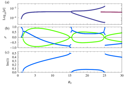
Figure 5: (a) Bifurcation diagram for the SIR model with $\beta_{1}=0.29$ and $\eta=10^{-6}$. (b) The Floquet multipliers, which are in general a complex conjugate pair, thus we plot the real (dark blue) and imaginary (light green) parts separately. (c) Imaginary parts of the Floquet exponents. Note that in the region where there are the coexisting limit cycles ($24<R_{0}<25$), only the multipliers/exponents for the biennial cycle are shown for clarity.

Figure 5 shows the bifurcation diagram for the model presented in the previous section, but with $\eta=10^{-6}$, along with the Floquet multipliers and exponents. These parameter values will be used for the rest of this section. Figure 6 shows the Floquet multipliers on a larger scale near the period doubling bifurcation point and figure 7 shows the analytical and numerical power spectra for various values of $R_{0}$ with $N=5\times 10^{6}$. Away from any bifurcation points there is good agreement between the analytic and the simulated spectra.

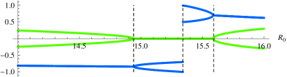
Figure 6: Floquet multipliers near to the period doubling bifurcation point, showing the virtual-Hopf pattern. For $R_{0}<14.94$ the multipliers are a complex conjugate pair, with a negative real part (dark blue line); this is the Hopf-like region. The actual period-doubling bifurcation occurs at $R_{0}^{\text{bif}}=15.34$, where one of the multipliers becomes equal to $-1$.

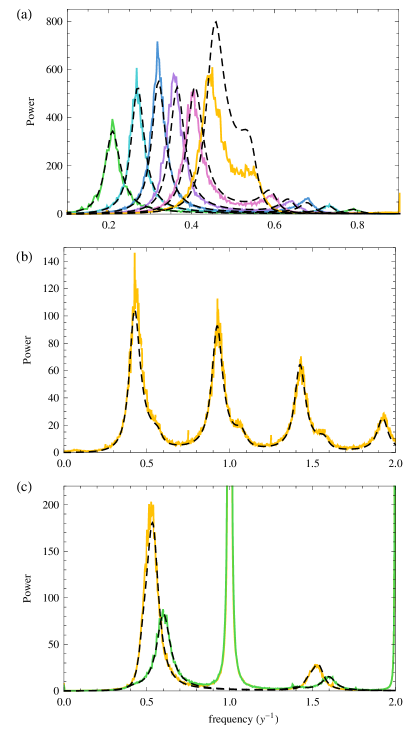
Figure 7: Analytic (black dashed curves) and numerical (coloured) power spectra for a range of $R_{0}$ with $N=5\times 10^{6}$. In most cases the analytic and numerical spectra are virtually indistinguishable, apart from $R_{0}=14$. (a) Spectra before the bifurcation, $R_{0}=4,6,8,10,12,14$. (b) Typical biennial regime, $R_{0}=20$. Note that the stochastic peaks have been made clearer by subtracting the deterministic dynamics before calculating the power spectrum. The spectrum would otherwise be dominated by the peak at $0.5$ y^-1. (c) The major and minor peaks in the large $R_{0}$ annual regime: $R_{0}=26,30$, with the larger peaks corresponding to $R_{0}=26$ for both the major and minor peaks.

As we approach the period-doubling bifurcation point from below, the stochastic oscillations follow a virtual-Hopf pattern (Wisenfeld, 1985a, b). This is where the oscillations first show the precursor characteristics of a Hopf bifurcation before changing into the precursor characteristics of a period-doubling. This is clearly seen in the power spectra shown in figure 7. In the Hopf-like regime ($R_{0}<14.94$), the Floquet multipliers are a complex conjugate pair, giving rise to two peaks in the spectrum: a major one at frequency Im$(\lambda)$ and a minor one at $1-$Im$(\lambda$), as in section 3. Therefore in figure 7a the two peaks are most widely separated for $R_{0}=4$.

As we increase $R_{0}$, ${\rm Im}(\lambda)$ also increases, and the major and minor peaks move closer together, converging at $0.5$ y^-1 when the multipliers become real and negative; this marks the onset of the period doubling regime, see figure 6. In this regime $(14.94<R_{0}<15.34$), as the multipliers are negative, so their phase is $\pm\pi$ and so the imaginary part of the Floquet exponents is $\pm\pi/2\pi T_{1}=\pm 0.5$. Therefore the peak stays fixed at $0.5$ years^-1 as we increase $R_{0}$ further within this range, but the amplitude increases quickly. At $R_{0}^{\text{bif}}=15.34$ one of the multipliers reaches $-1$ and we see a deterministic period doubling (Kuznetsov, 2004), and the size of the fluctuations grows to order $N$. Figure 8 shows how in this way the oscillations smoothly turn into the macroscopic biennial limit cycle. The same pattern is seen if we hold $R_{0}$ fixed and increase $\beta_{1}$ to induce a period doubling.

When the system is in the biennial regime we can still calculate the fluctuations about the limit cycle and get a good correspondence with analytic predictions (figure 7b). The positions of the peaks are now at $m/2\pm\text{Im}(\lambda)$ and the spectrum changes little within this parameter range. The peaks at $m/2+\text{Im}(\lambda)$ are barely visible, as compared to the prominent peaks at $m/2-\text{Im}(\lambda)$. In the annual regime after the doubling ($R_{0}>25$), the analytic results are again very accurate, with stochastic peaks at frequencies $m\pm\text{Im}(\lambda)$ (figure 7c). Here as well, the set of peaks at $m+\text{Im}(\lambda)$ are much smaller. Note that in both of these regions the time-series will be dominated by the deterministic signal as the stochastic oscillations are much smaller than in the pre-bifurcation region ($R_{0}<15$).

4.3 Near the bifurcation point

For values of $R_{0}$ near the bifurcation point, the deviations between the analytic and simulated spectra become larger (see for example figure 7a; $R_{0}=14$). This is expected: the analysis developed here is essentially linear and thus predicts an unbounded increase in the fluctuations as we approach the bifurcation point (Greenman and Benton, 2005). As the fluctuations become larger the linear approximation breaks down and non-linear effects become important and act to bound the fluctuations. Going to larger system sizes can result in better agreement between analytic results and simulation, but this will always break down at some point.

Although the analytic approximation breaks down near the bifurcation point, the structure we have uncovered is still visible. Figure 8 shows stochastic power spectra from simulations for $14<R_{0}<18$, as we move though the bifurcation point. The virtual-Hopf pattern is still clear, as predicted by the analysis, but the fluctuations remain bounded, growing to the same order as the system size (van Kampen, 1992; Kravtsov and Surovyatkina, 2003). Within this region the macroscopic dynamics cannot be split into a deterministic and stochastic part and it is not in general possible to reconstruct the deterministic part by averaging over many realisations. Thus, determining exactly where the bifurcation takes place is difficult (Wisenfeld, 1985b). At $R_{0}=16$ the deterministic biennial peak should be observed, but is not clearly visible until $R_{0}=18$. It is possible that the bifurcation point is shifted in the stochastic system, but more analysis is required to determine that this is so.

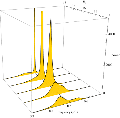
Figure 8: Simulation results showing how the power spectrum of the stochastic oscillations changes as the period doubling bifurcation point is crossed. The peaks for $R_{0}=17$ and $18$ have been cropped for clarity.

4.4 Smaller populations

The results presented in the previous sections were for $N=5\times 10^{6}$, which roughly corresponds to the largest populations we would be interested in modelling. Simulations of smaller populations tend to show regular deviations from the analytic calculations and results are sensitive to $N$, $\eta$ and $\beta_{1}$. The forcing pushes the system close to the fade-out boundary ($I=0$), where fluctuations are non-Gaussian, and so large deviations from the theory are expected. Figure 9 shows the stochastic power spectra from simulations, within the range $4\leq R_{0}\leq 30$ and with $N=5\times 10^{6},10^{6}$ and $5\times 10^{5}$.

For smaller values of $R_{0}$ we still clearly observe the virtual-Hopf pattern, but a visual inspection of the time-series shows much more irregular dynamics. This is due to the increased stochasticity in the smaller systems, but also the closeness of the fade-out boundary, where extinction and re-colonisation events start to have an impact on the dynamics (Griffiths, 1973). This has an effect on the power spectra in two ways: firstly as a broadening of the power spectra, showing a greater range or amplified frequencies and thus a more irregular dynamics. Secondly the endogenous period is systematically shifted higher, as in unforced versions of this model (Simoes et al., 2008). This reflects the fact that the period of oscillations also depends on the re-introduction of the disease after fade-out (Bartlett, 1957).

The most important effect is on the fluctuations in the biennial regime after the period doubling. For $N=5\times 10^{6}$ the peaks are sharp, indicating a deterministic limit cycle, and the stochastic oscillations are much smaller (figure 7b), hence the good predictability of these larger systems. For the two smaller populations this is not the case. We do not observe the deterministic biennial limit cycle, but instead see an enhanced stochastic peak and a broadening of the spectrum. The range of this enhanced region is also reduced.

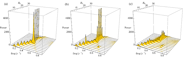
Figure 9: Power spectrum through the bifurcation point for different size populations. (a) $N=5\times 10^{6}$, (b) $N=10^{6}$, (c) $N=5\times 10^{5}$. Some of the peaks are cropped for clarity. Notice the anomalously enhanced peak for $N=10^{6}$, $R_{0}=10$, see section 4.5 for discussion of this.

Although there are large deviations, having an analytical description still helps us interpret the dynamics at smaller $N$. Taking the average of Eq. (9) we obtain

$$\langle I\rangle=N\psi(t)+N^{\frac{1}{2}}\langle y\rangle.$$ (17)

In the linear noise approximation, which we have used in this paper, the fluctuations are Gaussian and therefore $\langle y\rangle=0$. At some point this will break down and we must include the next order corrections, which will be of the order $N^{1/2}$, to the macroscopic equations. It will no longer be true that the mean is equal to the average (van Kampen, 1992; Grima, 2009). This effect of the fluctuations on the deterministic dynamics could be enough to retard the onset of the biennial limit cycle and is the subject of further research.

4.5 Switching between attractors

As seen from the bifurcation diagram in figure 5, where $\eta=10^{-6}$, the only region where deterministically there are predicted to be two coexisting states is when $24<R_{0}<25$. This can be detected in simulations and the period of switching depends strongly on the system size. If the system is large it will tend to stay in the state it started in, because the fluctuations are not large enough compared to the mean to kick the system into the other state. Decreasing the system size makes this possible, and we see periods of annual dynamics followed by biennial and back to annual, where the period of switching depends on the system size.

There is another intriguing region where we see signs of this type of behaviour. For $N=10^{6}$ and $R_{0}=10$ (figure 9b), we observe an enhanced stochastic peak in the spectrum with a period of 3 years. Visual inspection of the time-series shows regions of irregular annual oscillations interspersed with very regular triennial oscillations. Note that this is not observed in the larger or smaller systems and the power spectrum is shifted by the proximity to the fade-out boundary from its infinite system size limit. Very similar behaviour is observed for measles data from Baltimore between 1928 and 1935 (London and York, 1973; Earn et al., 2000), which has similar parameter values (Bauch and Earn, 2003b).

5 Discussion

We have used an analytic approach, as well as simulations, to quantify the effect of stochastic amplification in the forced SIR model. The time dependence has been treated explicitly, instead of by using an approximation as in a previous paper (Black and McKane, 2010). Because this model has a finite population, and therefore is inherently stochastic, it can only be studied ‘exactly’ by simulation. The system-size expansion, which we use to derive approximate analytic solutions for this model suggests that we should view the population-level dynamics as being composed of a deterministic part and a stochastic part, where the spectrum of the stochastic fluctuations is intimately related to the stability of the deterministic level dynamics. Power spectra of these models have been known for some time, but it has not always been clear what the mechanisms that generate the peaks are. This is the main advantage of being able to calculate the power spectrum of the stochastic fluctuations analytically; by comparison with the simulations we can gain insight into the mechanisms at work.

Our analysis suggests a simple explanation for the differences seen in the epidemic patterns of measles and whooping cough in England and Wales both before and after vaccination (Rohani et al., 1999), and which are representative of the two main parameter regimes for childhood diseases. The generic situation occurs when we are far away from the bifurcation point. Here we observe a deterministic annual limit cycle with stochastic oscillations, as in Figures 2 and 3. In general the form of the spectrum is close to that predicted by the unforced model. As already shown in a previous paper, this situation can account for the dynamics of whooping cough pre- and post-vaccination (Black and McKane, 2010). Pre-vaccination the stochastic oscillations are centred on 2-3 years. Vaccination acts to shift the endogenous frequency lower and increases the amplitude of these fluctuations giving large four yearly outbreaks.

Measles epidemics show a contrasting behaviour and represent the second important parameter regime, where the deterministic dynamics are near to a bifurcation point. Pre-vaccination, large cities such as London are in the regime with a deterministic biennial limit-cycle. Vaccination acts to lower $R_{0}$ and shift the system into the regime where there is an annual limit cycle with large stochastic oscillations. As vaccination coverage is increased, the endogenous period of these oscillations is also increased (Grenfell et al., 2001). Measles dynamics show a strong dependence on population size (Bartlett, 1957; Grenfell et al., 2002). Our analysis also offers some insight into this: in large populations the stochastic oscillations are very small compared with the deterministic biennial limit-cycle. This accounts for the regularity and explains why purely deterministic models capture this aspect so well (Dietz, 1976). For smaller populations the deterministic biennial limit-cycle is not observed, just enhanced stochastic oscillations, thus accounting for the more irregular dynamics seen in these smaller populations.

Finite size effects and immigration / imports are closely related in a stochastic individual-based model because the population is finite. Immigration reflects the basic fact that no population is isolated and there must be reintroduction of the disease if it fades out. One advantage of the approach which starts from an individual based model and derives the population level model, is that the immigration terms from the stochastic model are automatically included in the deterministic equations on the macro-scale. As we have shown, this is vital, as the longer period solutions are no longer found when they are included, and thus removes some speculation as to the influence of multiple co-existing attractors. These terms are easily omitted in a deterministic analysis because the system size is an innocent parameter (Nasell, 1999). It is interesting to note the similarities between immigration and age-structure in these forced models (Schenzle, 1984). Adding age-structure creates a constant pool of infectives in the infant class which acts to damp the dynamics (Bolker and Grenfell, 1993), exactly analogous to how we model immigration.

Owing to the importance of immigration in these epidemic systems one relevant outstanding question is: what form should the immigration parameter take? As measles dynamics can be highly synchronised it could be argued that the immigration parameter should reflect this (Bolker and Grenfell, 1995; Xia et al., 2004; Lloyd and Sattenspiel, 2009). On the other hand for larger cities, this parameter can be viewed as an aggregate of many infectious encounters from varied sources and could be approximated as a constant. Previous work has hinted at the sort of spatial effects that can arise (Keeling, 2000; Keeling and Rohani, 2002; Hagenaars et al., 2004), but investigation of explicitly spatial stochastic models should be a high priority.

The bifurcation diagrams for SEIR and SIR models are very similar, which justifies our use of the SIR model in this paper. The extension to uncoupled births and deaths would be straightforward, but would offer no further insight (Keeling and Rohani, 2007). There are technical difficulties in extending the method to the SEIR model because of the difference in time scales between the collapse onto the centre manifold (Schwartz and Smith, 1983) and the period of forcing; this creates difficulties in computing the Floquet multipliers. These could in principle be overcome either by calculating the multipliers by a different method (Fairgrieve and Jepson, 1991; Lust, 2001), or by carrying out a centre-manifold reduction before doing the van-Kampen expansion (Forgoston et al., 2009). The breakdown of the linear theory near the bifurcation point can be remedied by including next-to-leading order terms from the expansion of the master equation (van Kampen, 1992), but would result in a much more complex calculation. The calculations and discussions we have given here once again highlight the important role that simple models play in the understanding of complex systems. It also makes a novel contribution to the wider debate on the relative importance of stochastic and deterministic forces in ecology (Coulson et al., 2004).

Appendix A Expansion of the master equation

In this appendix we review the van Kampen system-size expansion, which approximates the master equation (8) by the deterministic equations (10) plus stochastic fluctuations given by Eq. (11) when $N$ is large. The method has been described by Alonso et al. (2007) for the SIR model without forcing (i.e. where $\beta$ is independent of time), where further details are given.

We begin by introducing step operators which allow us to express the master equation in a more compact form and also allow us to carry out the expansion in a more straightforward way. These are defined by:

$$\begin{split}\mathbb{E}_{I}^{\pm 1}\,f(S,I,t)=f(S,I\pm 1,t),\\ \mathbb{E}_{S}^{\pm 1}\,f(S,I,t)=f(S\pm 1,I,t).\end{split}$$ (18)

The master equation (8) can then be written in full as,

$$\frac{d}{dt}P(S,I,t)=\Biggl{\{} (\mathbb{E}_{S}\mathbb{E}^{-1}_{I}-1)\,\Bigl{[}\beta\frac{S}{N}I+\eta S\Bigr{]}$$ (19)

$$+(\mathbb{E}^{-1}_{S}-1)\,[\mu(N-S-I)]$$

$$+(\mathbb{E}_{I}\mathbb{E}_{S}^{-1}-1)\,[\mu I]+(\mathbb{E}_{I}-1)\,[\gamma I]\Biggr{\}}P(S,I,t),$$

which agrees with Alonso et al. (2007), up to typographical errors in that paper. The essential step in the expansion is the ansatz (9); we anticipate that the approximate probability distribution has a mean which scales as $N$ and width which scales as $N^{1/2}$ (van Kampen, 1992). To expand Eq. (19) in a power series in $N^{-1/2}$, we write the step operators in terms of the fluctuation variables $x$ and $y$:

$$\mathbb{E}_{S}^{\pm 1}=1\pm N^{-\frac{1}{2}}\frac{\partial}{\partial x}+\tfrac{1}{2}N^{-1}\frac{\partial^{2}}{\partial x^{2}}\pm\dotsb$$ (20)

$$\mathbb{E}_{I}^{\pm 1}=1\pm N^{-\frac{1}{2}}\frac{\partial}{\partial y}+\tfrac{1}{2}N^{-1}\frac{\partial^{2}}{\partial y^{2}}\pm\dotsb.$$

Substituting these and the ansatz (9) into Eq. (19) we identify a hierarchy of equations multiplied by different powers of $N^{-1/2}$. At leading order we find the deterministic equations (10) for the macroscopic variables, $\phi(t)$ and $\psi(t)$. At next-to-leading order we obtain a linear Fokker-Planck equation for the fluctuations variables $\mathbf{x}\equiv\{x,y\}$, of the form,

$$\frac{\partial\Pi}{\partial t}=-\sum_{i,j}K_{ij}(t)\frac{\partial[x_{j}\Pi]}{\partial x_{i}}+\frac{1}{2}\sum_{i,j}G_{ij}(t)\frac{\partial^{2}\Pi}{\partial x_{i}\partial x_{j}},$$ (21)

where the matrices $K(t)$ and $G(t)$ depend on time through $\beta(t)$, $\phi(t)$ and $\psi(t)$. The Fokker-Planck equation (21) is equivalent to the Langevin equations (11) given in the main text (van Kampen, 1992; Gardiner, 2003). Since we will not be interested in transient behaviour, only fluctuations about the limit cycle, the solutions to (10) will be those of the limit cycle, which we denote by $\bar{\phi}$ and $\bar{\psi}$. The explicit forms for $K(t)$ and $G(t)$ are then given by Eqs. (12) and (13) respectively. Since $\beta(t)$, $\bar{\phi}(t)$ and $\bar{\psi}(t)$ are periodic, so are $K(t)$ and $G(t)$.

Appendix B Floquet analysis

The analysis of the Langevin equation (11) is not difficult when the deterministic system approaches a fixed point at large times, and for the SIR model this is described by Alonso et al. (2007). When the attractor of the dynamics is a limit cycle, the analysis is more complicated, but can still be carried out to give the power spectra as integrals over known functions. Here we outline this analysis, following closely Boland et al. (2009), which may be consulted for further details.

We begin by considering linear perturbations about the limit cycle, that is, Eq. (11), but without the noise which originates from the discreteness of the individuals. The equation describing these small perturbations $\mathbf{x}\equiv\{x,y\}$ is

$$\dot{\mathbf{x}}=K(t)\mathbf{x},$$ (22)

where $K(t)$ is given by Eq. (12). A fundamental matrix, $X(t)$, is constructed from the linearly independent solutions of the homogeneous equation (22), thus it satisfies the relation,

$$\dot{X}(t)=K(t)X(t).$$ (23)

The matrix $X(t)$ is not unique and will depend on the initial conditions. Floquet theory states that if $K(t+T_{n})=K(t)$, then there exists a canonical fundamental matrix which can be expressed in the form $X_{0}(t)=P(t)Y(t)$ (Grimshaw, 1990). It has the property that the Floquet matrix, defined by $B_{0}=X_{0}^{-1}(0)X_{0}(T_{n})$, is diagonal. These diagonal elements are called Floquet multipliers, $\rho_{i}$ and play a central part in the theory. The matrix $P(t)$ carries the periodicity of the limit cycle, while $Y(t)=\text{diag}[e^{\lambda_{1}t},e^{\lambda_{2}t}]$, where $\lambda_{i}$ are the Floquet exponents. Using the periodicity of $P(t)$ it can be seen that $B=Y^{-1}(0)Y(T_{n})$ and so the Floquet multipliers are related to the Floquet exponents by $\rho_{i}=e^{\lambda_{i}T_{n}},i=1,2$. Using the canonical form, we can derive an expression for the power spectrum in terms of the matrices, $P(t)$ and $Y(t)$.

In practice, one obtains a fundamental matrix, $X(t)$ by numerically integrating (23) with initial condition $X(0)=\mathbb{I}$. With this choice of initial condition, $B=X(T_{n})$. The multipliers and exponents are then calculated from the the eigenvalues of $B$, which allows the construction of the matrix $Y(t)$, since the eigenvalues are independent of the choice of fundamental matrix. One can then calculate the canonical form, $X_{0}(t)=X(t)S$, where the columns of $S$ are the eigenvectors of $B$. Finally $P(t)$ is found from $P(t)=X(0)Y^{-1}(t)=X_{0}(t)Y(-t)$.

Having described the basic idea behind Floquet theory, we can now return to the Langevin equation (11), which is an inhomogeneous linear equation with periodic coefficients. We can use Floquet theory to construct a solution to this by adding a particular solution to the general solution of the corresponding homogeneous equation (22) (Grimshaw, 1990). This gives,

$$\mathbf{x}(t)=X(t)X^{-1}(t_{0})\mathbf{x}_{0}+X(t)\int_{t_{0}}^{t}X^{-1}(s)\mathbf{f}(s)ds,$$ (24)

with initial condition $\mathbf{x}(t_{0})=\mathbf{x}_{0}$. We are interested in the steady state solutions, when transients have damped down, thus we can ignore the first part of Eq. (24) and set the initial time to the infinite past, $t_{0}\rightarrow-\infty$. Taking the case where $X(t)$ is $X_{0}(t)=P(t)Y(t)$, one finds using the properties of the diagonal matrix $Y(t)$, that

$$\mathbf{x}(t)=P(t)\int_{-\infty}^{t}Y(t-s)P(s)^{-1}\mathbf{f}(s)ds.$$ (25)

The correlation matrix is defined as $C(t+\tau,t)=\langle\mathbf{x}(t+\tau)\mathbf{x}^{T}(t)\rangle$, which using Eq. (25) may be written as

$$C(t+\tau,t) = P(t+\tau)\int_{-\infty}^{t+\tau}\int_{-\infty}^{t}Y(t+\tau-s)P(s)^{-1}G(s)$$

$$\times \delta(s-s^{\prime})(P^{-1}(s^{\prime}))^{T}Y(t-s^{\prime})^{T}\,ds^{\prime}\,ds\,P(t)^{T},$$

where $\langle\mathbf{f}(s)\mathbf{f}^{T}(s^{\prime})\rangle=G(s)\delta(s-s^{\prime})$. Integrating over the delta function, the result will depend on the sign of $\tau$. If we take $\tau\geq 0$ then the integration region is $-\infty<s<t$, giving

$$C(t+\tau,t)=P(t+\tau)\int_{-\infty}^{t}Y(t+\tau-s)\Gamma(s)Y(t-s)^{T}\,ds\,P(t)^{T},$$ (27)

where we have defined

$$\Gamma(s)=P(s)^{-1}G(s)(P^{-1}(s))^{T},$$ (28)

which will have the periodicity of the limit cycle. Next we make a change of variables, $s\rightarrow t-s^{\prime}$, which gives

$$C(t+\tau,t)=P(t+\tau)\int_{0}^{\infty}Y(\tau+s^{\prime})\Gamma(t-s^{\prime})Y(s^{\prime})^{T}\,ds^{\prime}\,P(t)^{T}.$$ (29)

The form of $Y$ means we may write $Y(\tau+s^{\prime})=Y(\tau)Y(s^{\prime})$, and so the integral that we need to evaluate is given by

$$\Phi(t)\equiv\int_{0}^{\infty}Y(s)\Gamma(t-s)Y^{T}(s)\,ds.$$ (30)

Using the periodicity of the matrix $\Gamma(t-s)$, this integral can be recast as a finite one over the period of the limit cycle:

$$\Phi_{ij}=\frac{1}{1-\rho_{i}\rho_{j}}\int_{0}^{T_{n}}\Gamma_{ij}(t-s)e^{(\lambda_{i}+\lambda_{j})s}ds.$$ (31)

Therefore, the final expression for the correlation matrix is

$$C(t+\tau,t)=P(t+\tau)Y(\tau)\Phi(t)P(t)^{T}.$$ (32)

So we can obtain the correlation matrix as an integral, but this has to be evaluated numerically because the neither the limit-cycle solutions nor $P(t)$ can be obtained in closed form.

References

- Alonso et al. (2007) Alonso, D., McKane, A.J., Pascual, M., 2007. Stochastic amplification in epidemics. J. R. Soc. Interface 4, 575–582.
- Altizer et al. (2006) Altizer, S., Dobson, A., Hosseini P., Hudson, P., Pascual, M., Rohani, P., 2006. Seasonality and the dynamics of infectious diseases. Ecol. Lett. 9, 467–484.
- Anderson (2007) Anderson, D.F., 2007. A modified next reaction method for simulating chemical systems with time dependent propensities and delays. J. Chem. Phys. 127, 214107.
- Anderson et al. (1984) Anderson, R.M., Grenfell, B.T., May, R.M., 1984. Oscillatory fluctuations in the incidence of infectious disease and the impact of vaccination: time series analysis. J. Hyg. Camb. 93, 587–608.
- Anderson and May (1991) Anderson, R.M., May, R.M., 1991. Infectious diseases of humans: dynamics and control. Oxford University Press, Oxford.
- Aron and Schwartz (1984) Aron, J.L., Schwartz, I.B., 1984. Seasonality and period-doubling bifurcations in an epidemic model. J. Theo. Biol. 110, 665–679.
- Bartlett (1957) Bartlett, M.S., 1957. Measles periodicity and community size. J. R. Stat. Soc. Ser. A 120, 48–70.
- Bartlett (1960) Bartlett, M.S., 1960. Stochastic population models in ecology and epidemiology. Methuen, London.
- Bauch and Earn (2003a) Bauch, C.T., Earn, D.J.D., 2003a. Interepidemic intervals in forced and unforced SEIR models. Fields Inst. Comm. 36, 33–44.
- Bauch and Earn (2003b) Bauch, C.T., Earn, D.J.D., 2003b. Transients and attractors in epidemics. Proc. R. Soc. Lond. B 270, 1573–1578.
- Benton (2006) Benton, T.G., 2006. Revealing the ghost in the machine: using spectral analysis to understand the influence of noise on population dynamics. Proc. Natl. Acad. Sci. USA 103, 18387–18388.
- Black and McKane (2010) Black, A.J., McKane, A.J., 2010. Stochasticity in staged models of epidemics: quantifying the dynamics of whooping cough. J. R. Soc. Interface 7, 1219–1227.
- Boland et al. (2009) Boland, R.P., Galla, T., McKane, A.J., 2009. Limit cycles, complex Floquet multipliers and intrinsic noise. Phys. Rev. E 79, 051131.
- Bolker and Grenfell (1995) Bolker, B., Grenfell, B., 1995. Space, persistence and dynamics of measles epidemics. Phil. Trans. R. Soc. Lond. B 348, 309–320.
- Bolker and Grenfell (1993) Bolker, B.M., Grenfell, B.T., 1993. Chaos and biological complexity in measles dynamics. Proc. R. Soc. Lond. B 251, 75–81.
- Conlan et al. (2009) Conlan, A.J.K., Rohani, P., Lloyd, A.L., Keeling, M., Grenfell, B.T., 2009. Resolving the impact of waiting time distributions on the persistence of measles. J. R. Soc. Interface .
- Coulson et al. (2004) Coulson, T., Rohani, P., Pascual, M., 2004. Skeletons, noise and population growth: the end of an old debate? Trends Ecol. Evol. 19, 359–364.
- Dietz (1976) Dietz, K., 1976. The incidence of infectious diseases under the influence of seasonal fluctuations, in: Lecture notes in Biomathematics. Springer-Verlag. volume 11, pp. 1–15.
- Durrett and Levin (1994) Durrett, R., Levin, S.A., 1994. The importance of being discrete and spatial. Theo. Pop. Biol. 46, 363–394.
- Earn et al. (2000) Earn, D., Rohani, P., Bolker, B., Grenfell, B., 2000. A simple model for complex dynamical transitions in epidemics. Science 287, 667–670.
- Engbert and Drepper (1994) Engbert, R., Drepper, F., 1994. Chance and chaos in population biology - models of recurrent epidemics and food chain dynamics. Chaos, Solitons & Fractals 4, 1147–1169.
- Fairgrieve and Jepson (1991) Fairgrieve, T.F., Jepson, A.D., 1991. O.K. Floquet multipliers. SIAM J. Numer. Anal. 28, 1446–1462.
- Ferguson et al. (1996) Ferguson, N.M., Anderson, R.M., Garnett, G.P., 1996. Mass vaccination to control chickenpox: The influence of zoster. Proc. Natl. Adac. Sci. USA 93, 7231–7235.
- Forgoston et al. (2009) Forgoston, E., Billings, L., Schwartz, I.B., 2009. Accurate noise projection for reduced stochastic epidemic models. Chaos 19, 043110.
- Gardiner (2003) Gardiner, C.W., 2003. Handbook of stochastic methods. Springer. 3rd edition.
- Gillespie (1976) Gillespie, D., 1976. A general method for numerically simulating the stochastic time evolution of coupled chemical reactions. J. Comp. Phys. 22, 403–434.
- Greenman and Benton (2005) Greenman, J.V., Benton, T.G., 2005. The impact of environmental fluctuations on structured discrete time population models: resonance, synchrony and threshold behaviour. Theo. Pop. Biol. 68, 217–235.
- Grenfell et al. (2002) Grenfell, B., Bjornstad, O., Finkenstadt, B., 2002. Dynamics of measles epidemics: scaling noise, determinism and predictability with the TSIR model. Eco. Monographs 72, 185–202.
- Grenfell et al. (2001) Grenfell, B., Bjornstad, O.N., Keppey, J., 2001. Travelling waves and spatial hierarchies in measles epidemics. Nature 414, 716–723.
- Grenfell and Harwood (1997) Grenfell, B., Harwood, J., 1997. (Meta)population dynamics of infectious diseases. Trends Ecol. Evol. 12, 395–399.
- Griffiths (1973) Griffiths, D., 1973. The effect of measles vaccination on the incidence of measles in the community. J. R. Statist. Soc. A 136, 441.
- Grima (2009) Grima, R., 2009. Noise-induced breakdown of the Michaelis-Menten equation in steady-state conditions. Phys. Rev. Lett. 102, 218103.
- Grimshaw (1990) Grimshaw, R., 1990. Nonlinear ordinary differential equations. Blackwell, Oxford. 1st edition.
- Hagenaars et al. (2004) Hagenaars, T., Donnelly, C., Ferguson, N., 2004. Spatial heterogeneity and the persistence of infectious diseases. J. Theo. Biol. 229, 349–359.
- He and Earn (2007) He, D., Earn, D.J.D., 2007. Epidemiological effects of seasonal oscillations in birth rates. Theo. Pop. Biol. 72, 274–291.
- van Kampen (1992) van Kampen, N.G., 1992. Stochastic processes in physics and chemistry. Elsevier, Amsterdam.
- Keeling (2000) Keeling, M., 2000. Metapopulation moments: coupling, stochasticity and persistence. J. Ani. Ecol. 69, 725–736.
- Keeling and Rohani (2002) Keeling, M., Rohani, P., 2002. Estimating spatial coupling in epidemiological systems: a mechanistic approach. Ecol. Lett. 5, 20–29.
- Keeling and Rohani (2007) Keeling, M., Rohani, P., 2007. Modelling infectious diseases in humans and animals. Princeton University Press, Princeton.
- Keeling et al. (2001) Keeling, M., Rohani, P., Grenfell, B., 2001. Seasonally forced dynamics explored as switching between attractors. Physica D 148, 317–335.
- Kravtsov and Surovyatkina (2003) Kravtsov, Y.A., Surovyatkina, E.D., 2003. Nonlinear saturation of prebifurcation noise amplification. Phys. Lett. A 319, 348–351.
- Kuznetsov (2004) Kuznetsov, Y.A., 2004. Elements of applied bifurcation theory. Springer, New York. 3rd edition.
- Kuznetsov and Piccardi (1994) Kuznetsov, Y.A., Piccardi, C., 1994. Bifurcation analysis of periodic SEIR and SIR epidemic models. J. Math. Biol. 32, 109–121.
- Lloyd and Sattenspiel (2009) Lloyd, A.L., Sattenspiel, L., 2009. Spatiotemporal dynamics of measles: synchrony and persistence in a disease metapopulation, in: Spatial Ecology. CRC Press, pp. 251–272.
- London and York (1973) London, W.P., York, J.A., 1973. Recurrent outbreaks of measles, chickenpox and mumps I: Seasonal variation in contact rates. Am. J. Epidemiology 98, 453–468.
- Lust (2001) Lust, K., 2001. Improved numerical Floquet multipliers. Int. J. Bifurcation and Chaos 11, 2389–2410.
- McKane and Newman (2005) McKane, A.J., Newman, T.J., 2005. Predator-prey cycles from resonant amplification of demographic stochasticity. Phys. Rev. Lett. 94, 218102.
- Nasell (1999) Nasell, I., 1999. On the time to extinction in recurrent epdemics. J. R. Stat. Soc. B 61, 309–330.
- Nasell (2002) Nasell, I., 2002. Measles outbreaks are not chaotic, in: Mathematical approaches for emerging and reemerging infectious diseases: models, methods and theory. Springer-Verlag, pp. 85–114.
- Nguyen and Rohani (2008) Nguyen, H.T.H., Rohani, P., 2008. Noise, nonlinearity and seasonality: the epidemics of whooping cough revisited. J. R. Soc. Interface 5, 403–413.
- Nisbet and Gurney (1982) Nisbet, R., Gurney, W., 1982. Modelling fluctuating populations. Wiley, New York.
- Olsen et al. (1988) Olsen, L.F., Truty, G.L., Schaffer, W.M., 1988. Oscillations and chaos in epidemics: a nonlinear dynamic study of six childhood diseases in Copenhagen, Denmark. Theo. Pop. Bio. 33, 344–370.
- Priestley (1982) Priestley, M.B., 1982. Spectral analysis and time series. Academic Press, London.
- Rand and Wilson (1991) Rand, D.A., Wilson, H.B., 1991. Chaotic stochasticity - a ubiquitous source of unpredictability in epidemics. Proc. R. Soc. Lond. B 246, 179–184.
- Rohani et al. (1999) Rohani, P., Earn, D.J.D., Grenfell, B.T., 1999. Opposite patterns of synchrony in sympatric disease metapopulations. Science 286, 968–971.
- Rohani et al. (2002) Rohani, P., Keeling, M.J., Grenfell, B.T., 2002. The interplay between determinism and stochasticity in childhood diseases. Am. Nat. 159, 469–481.
- Schenzle (1984) Schenzle, D., 1984. An age-structured model of pre- and post-vaccination measles transmission. Math. Med. Biol. 1, 169–191.
- Schwartz (1985) Schwartz, I.B., 1985. Multiple stable recurrent outbreaks and predictability in seasonally forced nonlinear epidemic models. J. Math. Biol. 21, 347–361.
- Schwartz and Smith (1983) Schwartz, I.B., Smith, H.L., 1983. Infinite subharmonic bifurcation in an SEIR epidemic model. J. Math. Biol. 18, 233–253.
- Simoes et al. (2008) Simoes, M., Telo da Gama, M.M., Nunes, A., 2008. Stochastic fluctuations in epidemics on networks. J. R. Soc. Interface 5, 555–566.
- Wisenfeld (1985a) Wisenfeld, K., 1985a. Noisy precursors of nonlinear instabilities. J. Stat. Phys. 38, 1071–1097.
- Wisenfeld (1985b) Wisenfeld, K., 1985b. Virtual Hopf phenomenon: a new precursor of period-doubling bifurcations. Phys. Rev. A 32, 1744–1751.
- Wolfram Research (2008) Wolfram Research, 2008. Mathematica. Wolfram Research Inc., Champaign, Illinois. Version 7.
- Xia et al. (2004) Xia, Y., Bjornstad, O.N., Grenfell, B.T., 2004. Measles metapopulation dynamics: a gravity model for epidemiological coupling and dynamics. Am. Nat. 164, 267–281.