Anisotropic conductivity of doped graphene
due to short-range non-symmetric scattering

Abstract

The conductivity of doped graphene is considered taking into account scattering by short-range nonsymmetric defects, when the longitudinal and transverse components of conductivity tensor appear to be different. The calculations of the anisotropic conductivity tensor are based on the quasiclassical kinetic equation for the case of monopolar transport at low temperatures. The effective longitudinal conductivity and the transverse voltage, which are controlled by orientation of sample and by gate voltage (i.e. doping level), are presented.

The conductivity tensor $\sigma_{\alpha\beta}$ is determined both by the symmetry properties of carriers and by the character of scattering processes. For a medium with cubic (quadratic for the 2D case) symmetry, the conductivity appears to be a scalar, i. e. $\sigma_{\alpha\beta}\propto\delta_{\alpha\beta}$. 1 Anisotropic conductivity of hot electrons in low-symmetric bulk materials (Ge and Si) were studied over 50 years ago. 2 For the hexagonal symmetry case, which is correspondent to an ideal graphene sheet, the longitudinal (along $X$-axis, see Fig. 1) and transverse conductivities of hot carriers appear to be different. This anisotropic conductivity appears due to the trigonal warping of energy spectrum 3 even for the isotropic scattering case. Such an anisotropy is weak [$\propto(a\bar{p}/\hbar)^{2}$, where $a$ is the lattice constant and $\bar{p}$ is the characteristic momentum] and it can be essential for the high-energy carriers, at energies $\geq 1.5$ eV. In the linear regime, the anisotropy of conductivity is possible due to scattering by short-range nonsymmetric defects, see Fig. 1b where a substitutional impurity is shown. Although the nonsymmetric defects were discussed in Refs. 4-7, the anisotropy of conductivity was not theoretically analyzed or mentioned. To date, no experimental data are reported concerning any mechanism of anisotropy listed; so that, a study of this phenomena is timely now.

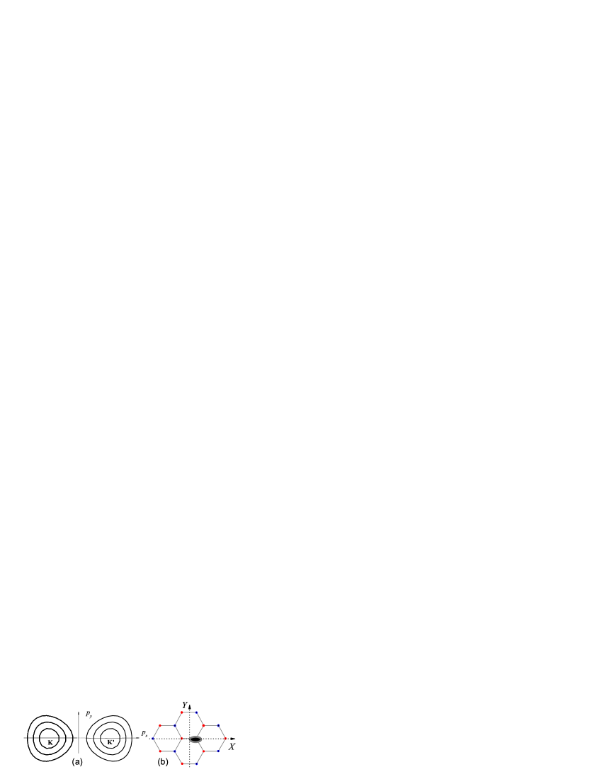
Figure 1: (Color online) (a) Equal enegry contours around the $K$ and $K^{\prime}$ points with step 0.5 eV; a visible anisotropy takes place at energies $\geq 1.5$ eV. (b) Graphene sheet with a short-range nonsymmetric defect marked by ellipse.

In this Letter, we consider the low-temperature conductivity taking into account both the long-range isotropic disorder (see 8 ; 9 ; 10 ) and the short-range nonsymmetric defects (see 4 ; 5 ; 6 ; 7 ). The longitudinal and transverse components of conductivity tensor are calculated based on the linearized Boltzmann equation with the transition probabilities written in the Born approximation. The effective conductivity and the transverse voltage of a graphene strip are presented for the case of weak anisotropy and their dependencies on carrier’s concentration (gate voltage) and on orientation of strip are discussed.

We consider the momentum relaxation in graphene which is caused by the interaction of carriers with a weak potential $\sum_{j}\hat{U}({\bf x}-{\bf x}_{j})$, where ${\bf x}_{j}$ is the coordinate of $j$th impurity ($j=1,\ldots N_{im}$ and $N_{im}$ is the number of impurities over the normalization area $L^{2}$). The potential of a single impurity placed at ${\bf x}=0$ is given by $\hat{U}({\bf x})=v_{\bf x}+\hat{u}\delta({\bf x})$; here we separated the long-range scalar contribution, $v_{\bf x}$, and the short-range addend determined by the $4\times 4$ matrix $\hat{u}$. For a nonmagnetic defect, this matrix should be Hermitian and time-reversal symmetric and one can write $\hat{u}$ using 9 independent real parameters $u_{sl}$:

$$\hat{u}=\sum\limits_{s,l=x,y,z}u_{sl}\hat{\Sigma}_{s}\hat{\Lambda}_{l},$$ (1)

where $4\times 4$ matrices $\Sigma_{s}$ and $\Lambda_{l}$ are introduced in Refs. 4-6. In the framework of the Born approximation, the transition probability between the $c$-band states $|\eta^{\prime}{\bf p}^{\prime}\rangle$ and $|\eta{\bf p}\rangle$ is given by

$$W_{\eta^{\prime}{\bf p}^{\prime}\eta{\bf p}}=\frac{2\pi}{\hbar}\frac{n_{im}}{L^{2}}\left|\left\langle\eta^{\prime}{\bf p}^{\prime}\left|{\hat{U}}\right|\eta{\bf p}\right\rangle\right|^{2}\delta\left(\varepsilon_{p^{\prime}}-\varepsilon_{p}\right),$$ (2)

where $\bf p$ is 2D momentum, $n_{im}=N_{im}/L^{2}$ is the impurity concentration, $\eta=K,K^{\prime}$ is correspondent to $K$- or $K^{\prime}$-valleys and the linear dispersion law $\varepsilon_{p}=v_{W}p$ is not dependent on $\eta$ ($v_{W}=10^{8}$ cm/s is the characteristic velocity). 3 Below we restrict ourselves by the case of weak short-range corrections to the long-range scattering contribution. As a result, one obtains the intravalley matrix element in (2) as

$$\left|\left\langle K{\bf p}^{\prime}\left|{\hat{U}}\right|K{\bf p}\right\rangle\right|^{2}\simeq v_{q}^{2}\frac{1-\cos\Delta\varphi}{2}$$ (3)

$$+\frac{u_{xz}^{2}}{2}\left[1+\cos\left(\varphi+\varphi^{\prime}\right)\right]+\frac{u_{yz}^{2}}{2}\left[1-\cos\left(\varphi+\varphi^{\prime}\right)\right],$$

where the main contribution is written through the Fourier component of $v_{\bf x}$, which is dependent on the momentum transfer $\hbar{\bf q}={\bf p}-{\bf p}^{\prime}$, and through the factor $(1-\cos\Delta\varphi)$ with $\Delta\varphi=\widehat{{\bf p}^{\prime},{\bf p}}$ described the suppression of backscattering processes. The $\Delta\varphi$-dependent contributions, which are proportional to $u_{sl}^{2}$, were omitted in Eq. (3). In addition, a weak $\Delta\varphi$-dependent intervalley matrix element, which is proportional to $u_{zl}^{2}$ or to $u_{sl}^{2}$ with $(s,l)\to(x,y)$ should also be neglected. The remaining corrections in Eq. (3), which are dependent on $\varphi+\varphi^{\prime}$ ($\varphi$ and $\varphi^{\prime}$ are the polar angles of $\bf p$ and ${\bf p}^{\prime}$), are responsible for the anisotropic conductivity under consideration if $u_{xz}^{2}\neq u_{yz}^{2}$, i.e. scattering processes along $X$- and $Y$-directions are different.

Next, we solve the Boltzmann kinetic equation linearized with respect to the steady-state electric field $\bf E$. Taking into account that the transition probability given by Eqs. (2), (3) does not dependent on $\eta$ and that $W_{\bf pp^{\prime}}=W_{\bf p^{\prime}p}$, we write the kinetic equation for the anisotropic part of distribution $\Delta f_{\bf p}$, which is $\propto{\bf E}$, in the following form:

$$e\left({\bf E}\cdot{\bf v}_{\bf p}\right)\frac{df_{\varepsilon}}{d\varepsilon}=\sum\limits_{{\bf p}^{\prime}}W_{{\bf p}^{\prime}{\bf p}}\left(\Delta f_{{\bf p}^{\prime}}-\Delta f_{\bf p}\right).$$ (4)

Here ${\bf v}_{\bf p}=\nabla_{\bf p}\varepsilon_{p}$ is the velocity, $f_{\varepsilon}$ is the equilibrium distribution and $df_{\varepsilon}/d\varepsilon\simeq-\delta(\varepsilon_{F}-\varepsilon_{p})$ for the degenerate carriers with the Fermi energy $\varepsilon_{F}$. We solve the integral equation (4) using the variational approach 11 with the trial distribution function $\Delta f_{\bf p}=e\left({\bf C}\cdot{\bf v}_{\bf p}\right)\delta(\varepsilon_{F}-\varepsilon_{p})$. An unknown vector $\bf C$ is determined from the extremum conditions for the quadratic form:

$${\cal K}({\bf C})=\left({\bf C}\cdot\hat{A}\cdot{\bf E}\right)+\left({\bf C}\cdot\hat{L}\cdot{\bf C}\right),$$ (5)

where the field-dependent contribution is determined by the tensor:

$$A_{\alpha\beta}=\frac{2\upsilon_{W}^{2}}{L^{2}}\sum\limits_{\bf p}{\delta(\varepsilon_{F}-\varepsilon_{p})\frac{{p_{\alpha}p_{\beta}}}{{p^{2}}}=\delta_{\alpha\beta}}\frac{\upsilon_{W}^{2}\rho_{F}}{4}$$ (6)

written through the density of states at the Fermi energy, $\rho_{F}$. The collision-induced contribution in Eq. (5) is determined by the matrix:

$$L_{\alpha\beta}=\frac{2\pi n_{im}\upsilon_{W}^{2}}{{\hbar L^{4}}}\sum\limits_{{\bf pp}^{\prime}}\left|\left\langle K{\bf p}^{\prime}\left|{\hat{U}}\right|K{\bf p}\right\rangle\right|^{2}\delta(\varepsilon_{F}-\varepsilon_{p})$$

$$\times\delta(\varepsilon_{F}-\varepsilon_{p^{\prime}})\frac{p_{\alpha}(p^{\prime}_{\beta}-p_{\beta})}{p^{2}}$$ (7)

and after substitution of the matrix elements (3) one obtains $L_{\alpha\beta}=0$ if $\alpha\neq\beta$. The diagonal components of Eq. (7) take form:

$$L_{\alpha\alpha}\simeq\frac{\pi n_{im}\upsilon_{W}^{2}\rho_{F}^{2}v_{0}^{2}}{8\hbar}\left[\Psi\left(\frac{p_{F}l_{c}}{\hbar}\right)\pm\frac{u_{xz}^{2}-u_{yz}^{2}}{8v_{0}^{2}}\right],$$ (8)

where $+$ (or $-$) is correspondent to $L_{xx}$ (or $L_{yy}$). The factor $v_{0}^{2}\Psi(p_{F}l_{c}/\hbar)$ appears here due to the long-range part of potential ($v_{0}\equiv v_{q=0}$) with the correlation lenth $l_{c}$. The function $\Psi(p_{F}l_{c}/\hbar)$ was introduced in 9 for the case of the finite-range potential with Gaussian correlations.

The current density is given by ${\bf I}=(4e/L^{2})\sum_{\bf p}{\bf v}_{\bf p}\Delta f_{\bf p}$, where the factor 4 is due to the spin and valley degeneracy. Since $\Delta f_{\bf p}\propto{\bf C}\propto{\bf E}$, the conductivity tensor $\hat{\sigma}$ is introduced as ${\bf I}=\hat{\sigma}{\bf E}$. Substituting $\Delta f_{\bf p}$ into $\bf I$ and performing integration over $\bf p$, one obtains ${\bf I}=(ev_{W})^{2}{\bf C}\rho_{F}/2$, where $\bf C$ is determined from the extremum conditions which give the linear equations: $\partial{\cal K}({\bf C})/\partial C_{\alpha}=0$ for $\alpha=x,y$. As a result, one obtains the diagonal tensor $\sigma_{\alpha\alpha}=\overline{\sigma}\pm\delta\sigma/2$, where $+$ (or $-$) is correspondent to $\sigma_{xx}$ (or $\sigma_{yy}$). Here the isotropic part of conductivity $\overline{\sigma}$ and the anisotropic correction $\delta\sigma$ are given by

$$\overline{\sigma}\simeq\frac{e^{2}}{\hbar}\frac{(\upsilon_{W}\hbar)^{2}}{2\pi n_{im}v_{0}^{2}\Psi(p_{F}l_{c}/\hbar)},$$

$$\delta\sigma\simeq-\frac{\overline{\sigma}}{\Psi(p_{F}l_{c}/\hbar)}\frac{u_{xz}^{2}-u_{yz}^{2}}{8v_{0}^{2}},$$ (9)

so that the anisotropy of conductivity is determined by the dimensionless factor $(u_{xz}^{2}-u_{yz}^{2})/(8v_{0}^{2})$.

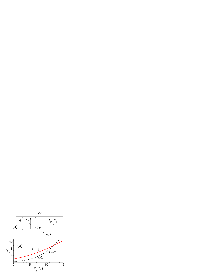
Figure 2: (Color online) (a) Graphene strip of width $d$ with angle $\theta$ to $X$-direction (dotted arrows are correspondent to the $X0Y$ coordinate system). Longitudinal and transverse fields, $E_{\bot}$ and $E_{\|}$, as well as longitudinal current $I_{\|}$ are shown. (b) Functions $\Psi^{-1}$ and $\Psi^{-2}$ which describe gate voltage dependencies of transverse voltage, $E_{\bot}/E_{\|}$, and of anisotropic contribution to conductivity, $(\sigma_{eff}-\overline{\sigma})$, given by Eq. (10).

Using the conductivity tensor determined by Eqs. (9), we consider the conductivity of strip, see Fig. 2a where $d$ is the width of strip and $\theta$ is the angle between its orientation and $X$-axis. Since the absence of the transverse current, $I_{\bot}=0$, the linear relation ${\bf I}=\hat{\sigma}{\bf E}$ permits one to calculate the effective conductivity, which is introduced according to $I_{\|}=\sigma_{eff}E_{\|}$, and the induced transverse voltage, $E_{\bot}d$. For the weak anisotropy case, we obtain the simple angle dependencies

$$\frac{E_{\bot}}{E_{\|}}\simeq\frac{\delta\sigma}{\overline{\sigma}}\sin 2\theta,~{}~{}~{}~{}\sigma_{eff}-\overline{\sigma}\simeq\frac{\delta\sigma}{2}\cos 2\theta$$ (10)

and maximal values of the transverse voltage $|E_{\bot}/E_{\|}|$ and of the anisotropic contributions to $\sigma_{eff}$ appear at $\theta=\pi/4$, $3\pi/4,\ldots$ and at $\theta=0$, $\pi/2,\ldots$, respectively. The concentration (or gate voltage, $V_{g}$) dependencies are determined through the function $\Psi(p_{F}l_{c}/\hbar)$ introduced in Eqs. (8), (9). According to Eq. (10), one obtains $|E_{\bot}/E_{\|}|\propto\Psi^{-1}$ and $\delta\sigma\propto\Psi^{-2}$; we plot these functions in Fig. 2b for the graphene strip placed over the SiO₂ substrate of 300 nm width. We also use $l_{c}\simeq$10 nm in agreement with experimental data, see Ref. 9. Since the function $\Psi$ decreases with $V_{g}$, both the transverse voltage $|E_{\bot}/E_{\|}|$ and the anisotropy of conductivity $(\sigma_{eff}-\overline{\sigma})$ increase with $V_{g}$; notice, that the anisotropy of conductivity increases more faster (about 10 times at $V_{g}\simeq$10 V) because $\delta\sigma\propto\Psi^{-2}$. The transverse field and the anisotropy of effective conductivity given by Eq. (10) are proportional to the unknown parameter $(u_{xz}^{2}-u_{yz}^{2})/(8v_{0}^{2})$ and a value of the anisotropy effect is not estimated here. However, these results permit one to verify a mechanism of anisotropy using the gate voltage and angle dependencies obtained. In addition, a ratio $(u_{xz}^{2}-u_{yz}^{2})/(8v_{0}^{2})$ can be measured. Supposing $(u_{xz}^{2}-u_{yz}^{2})/(8v_{0}^{2})\sim 10^{-2}$, one obtains that $|E_{\bot}/E_{\|}|$ and $|\delta\sigma/\overline{\sigma}|$ are about 10 %.

Further, we discuss the assumptions used. The consideration performed is based on the simplified description of scattering with separated long- and short-range parts of potential. The parameters of long-range scattering are determined from the phenomenological consideration 9 while the short-range contribution is expressed through unknown matrix $\hat{u}$, without verification of a microscopical nature of defects. The variational solution of Eq. (4) gives a good estimation of the anisotropy under consideration. The results (10) do not dependent on a width of strip if $d$ exceeds the mean free path due to the long-range scattering, so that an edge scattering is not essential under the condition $d\gg$0.1 $\mu$m (here we used the results for non-ideal nanoribbons 12 ). We also restrict ourselves by the degenerate carriers case because the anisotropy effects increase with concentration (or gate voltage). The rest of assumptions (quasiclassical kinetic equation, weak acoustic phonon scattering, and model description of long-range scattering 9 ) are rather standard.

In conclusion, we have demonstrated that the nonsymmeric short-range scattering gives rise to the transverse voltage and to the orientation-dependent effective conductivity of graphene strip. These dependencies permit one to measure asymmetry of scattering which is expressed through the characteristics of short-range defect. We believe that these results will stimulate further measurements of anisotropy and microscopical calculations of nonsymmetric defects. Beside this, a nonequivalent heating of carriers in different valleys (and an intervalley redistribution of carriers) by a strong electric field takes place under an essential anisotropy of scattering (in analogy with the bulk case 13 ).

I am grateful to E. I. Karp for a useful comment.

References

- (1) J. F. Nye, Physical Properties of Crystals, (Oxford Univ. Press, Oxford 1995).
- (2) W. Sasaki, M. Shibuya and K. Mizuguchi, J. Phys. Soc. Jpn. 13, 456 (1958).
- (3) A.H. Castro Neto, F. Guinea, N.M.R. Peres, K.S. Novoselov, and A.K. Geim, Rev. Mod. Phys. 81, 109 (2009).
- (4) E. McCann, K. Kechedzhi, V. I. Falko, H. Suzuura, T. Ando, and B. L. Altshuler, Phys. Rev. Lett. 97, 146805 (2006); V. V. Cheianov and V. I. Falko, Phys. Rev. Lett. 97, 226801 (2006).
- (5) I. L. Aleiner and K. B. Efetov, Phys. Rev. Lett. 97, 236801 (2006).
- (6) E. Mariani, L. I. Glazman, A. Kamenev, and F. von Oppen, Phys. Rev. B 76 165402 (2007).
- (7) V. M. Pereira, J. M. B. Lopes dos Santos, and A. H. Castro Neto, Phys. Rev. B 77 115109 (2008); B. Dora, K. Ziegler, and P. Thalmeier, Phys. Rev. B 77 115422 (2008).
- (8) N.M.R. Peres, J.M.B. Lopes dos Santos, and T. Stauber, Phys. Rev. B 76, 073412 (2007); T. Stauber, N.M.R. Peres, and F. Guinea, Phys. Rev. B 76, 205423 (2007).
- (9) F.T. Vasko and V. Ryzhii, Phys. Rev. B 76, 233404 (2007).
- (10) S. Adam, E.H. Hwang, E. Rossi, S. Das Sarma, Solid State Comm. 149, 1072 (2009).
- (11) J.M. Ziman, Electrons and Phonons (Qxford University Press, Qxford 2001).
- (12) M. Evaldsson, I. V. Zozoulenko, H. Xu and T. Heinzel, Phys. Rev. B 78, 161407 (2008); M. Y. Han, B. Ozyilmaz, Y. Zhang, and P. Kim, Phys. Rev. Lett. 98, 206805 (2007).
- (13) M. Asche and O. G. Sarbei, Phys. Stat. Sol. 33, 9 (1969).