Particle-Hole Optical Model: Fantasy or Reality?

Abstract

An attempt to formulate the optical model of particle-hole-type excitations (including giant resonances) is undertaken. The model is based on the Bethe–Goldstone equation for the particle-hole Green function. This equation involves a specific energy-dependent particle-hole interaction that is due to virtual excitation of many-quasiparticle configurations and responsible for the spreading effect. After energy averaging, this interaction involves an imaginary part. The analogy between the single-quasiparticle and particle-hole optical models is outlined.

Damping of giant resonances (GRs) is a long-standing problem for theoretical studies. There are three main modes of GR relaxation: (i) particle-hole (p–h) strength distribution (Landau damping), which is a result of the shell structure of nuclei; (ii) coupling of (p–h)-type states with the single-particle (s.p.) continuum, which leads to direct nucleon decay of GRs; and, (iii) coupling of (p–h)-type states with many-quasiparticle configurations, which leads to the spreading effect. An interplay of these relaxation modes takes place in the GR phenomenon.

A description of the giant-resonance strength function with exact allowance for the Landau damping and s.p. continuum can be obtained within the continuum-RPA (cRPA), provided the nuclear mean field and p–h interaction are fixed ref1 . As for the spreading effect, it is attempted to be described together with other GR relaxation modes within microscopic and semimicroscopic approaches. The coupling of the (p–h)-type states, which are the doorway states (DWS) for the spreading effect, with a limited number of 2p–2h configurations is explicitly taken into account within the microscopic approaches (see, e.g., Refs. ref2 ; ref3 ). Some questions to the basic points of these approaches could be brought up: (i) “Thermalization” of the DWS, which form a given GR, i.e. the DWS coupling with many-quasiparticle states (MQPS) (the latter are complicated superpositions of 2p–2h, 3p–3h, …configurations), is not taken into account. As a result, each DWS may interact with others via 2p–2h configurations. Due to complexity of MQPS one can reasonably expect that after energy averaging the interaction of different DWS via MQPS would be close to zero (the statistical assumption). (ii) The use of a limited basis of 2p–2h configurations does not allow to describe correctly the GR energy shift due to the spreading effect. The full basis of these configurations should be formally used for this purpose. (iii) With the single exception of Ref. ref4 , there are no studies of GR direct-decay properties within the microscopic approaches.

Within the so-called semimicroscopic approach, the spreading effect is phenomenologically taken into account directly in the cRPA equations in terms of the imaginary part of an effective s.p. optical-model potential ref5 ; ref6 . Within this approach, the afore-mentioned statistical assumption is supposed to be valid and used in formulation of the approach. The GR energy shift due to the spreading effect is evaluated by means of the proper dispersive relationship, and therefore, the full basis of MQPS is formally taken into account ref7 . The approach is applied to description of direct-decay properties of various GRs (the references are given in Ref. ref6 ). In accordance with the “pole” approximation used for description of the spreading effect within the semimicroscopic approach, the latter is valid only in the vicinity of the GR energy. However, for an analysis of some phenomena it is necessary to describe the low- and/or high-energy tails of various GRs. For instance, the asymmetry (relative to 90^∘) of the ($\gamma\mathrm{n}$)–reaction differential cross section at the energy of the isovector giant quadrupole resonance is determined, in particular, by the high-energy tail of the isovector giant dipole resonance ref8 . Another example is the isospin-selfconsistent description of the IAR damping. In particular, the IAR total width is determined by the low-energy tail of the charge-exchange giant monopole resonance ref9 ; ref9_5 ; ref10 .

In the present work, we attempt to formulate a model for phenomenological description of the spreading effect on p–h strength functions at arbitrary (but high enough) excitation energies. The formulation of this semimicroscopic model (simply called as the p–h optical model) is analogous to that of the single-quasiparticle optical model ref11 ; ref12 . The dispersive version of this model ref11 is widely used for description of various properties of single-quasiparticle excitations at relatively high energies (see, e.g., Ref. ref13 ). This model can be also used for description of direct particle decay of subbarrier s.p. states ref14 .

The starting point in formulation of the single-quasiparticle optical model is the Fourier-component of the Fermi-system single-quasiparticle Green function, $G(x,x^{\prime};\varepsilon)$, taken in the coordinate representation (see, e.g., Refs. ref11 ; ref12 ). By analogy with that, we start formulation of the p–h optical model from the Fourier-component of the Fermi-system (generally, nonlocal) p–h Green function, $\mathcal{A}(x,x^{\prime};x_{1},x^{\prime}_{1};\omega)$, also taken in the coordinate representation. Being a kind of the Fermi-system two-particle Green function (definitions see, e.g., in Ref. ref15 ), $\mathcal{A}$ satisfies the following spectral expansion:

$$\mathcal{A}(x,x^{\prime};x_{1},x^{\prime}_{1};\omega)=\sum_{s}\left(\frac{\rho_{s}^{\ast}(x^{\prime},x)\rho_{s}(x_{1},x^{\prime}_{1})}{\omega-\omega_{s}+i0}-\frac{\rho_{s}^{\ast}(x^{\prime}_{1},x_{1})\rho_{s}(x,x^{\prime})}{\omega+\omega_{s}-i0}\right).$$ (1)

Here, $\omega_{s}=E_{s}-E_{0}$ is the excitation energy of an exact state $|s\rangle$ of the system and $\rho_{s}(x,x^{\prime})=\langle s|\widehat{\Psi}^{+}(x)\widehat{\Psi}(x^{\prime})|0\rangle$ is the transition matrix density ($\widehat{\Psi}^{+}(x)$ is the operator of particle creation at the point $x$). In accordance with the expansion of Eq. (1) the p–h Green function determines the strength function $S_{V}(\omega)$ corresponding to an external (generally, nonlocal) single-quasiparticle field $\widehat{V}=\int\widehat{\Psi}^{+}(x)V(x,x^{\prime})\widehat{\Psi}(x^{\prime})dxdx^{\prime}\equiv\left[\widehat{\Psi}^{+}V\widehat{\Psi}\right]$:

$$S_{V}(\omega)=-\frac{1}{\pi}\mathrm{Im}\left[V^{+}\mathcal{A}(\omega)V\right],$$ (2)

where the brackets $\left[\dots\right]$ mean the proper integrations.

The free s.p. and p–h Green functions, $G_{0}(x,x^{\prime};\varepsilon)$ and $\mathcal{A}_{0}(x,x^{\prime};x_{1},x^{\prime}_{1};\omega)$, respectively, are determined by the mean field (via the single-quasiparticle wave functions) and the occupation numbers (only nuclei without nucleon pairing are considered). Being determined by Eq. (1), the free transition matrix densities $\rho_{s}^{(0)}(x,x^{\prime})$ are orthogonal: $\left[\rho_{s}^{(0)\ast}\rho_{s^{\prime}}^{(0)}\right]=\delta_{ss^{\prime}}$. As for the transition densities $\rho_{s}^{(0)}(x=x^{\prime})$, which appear in the spectral expansion for the free local p–h Green function $A_{0}(x,x_{1};\omega)=\mathcal{A}_{0}(x=x^{\prime},x_{1}=x_{1}^{\prime};\omega)$, this statement is wrong. The RPA p–h Green function, $\mathcal{A}_{RPA}(x,x^{\prime};x_{1},x^{\prime}_{1};\omega)$, is determined also by a p–h (local) interaction $\mathcal{F}(x,x^{\prime};x_{1},x^{\prime}_{1})=F(x,x_{1})\delta(x-x^{\prime})\delta(x_{1}-x^{\prime}_{1})$, which is responsible for long-range correlations leading to formation of GRs. In particular, the Landau–Migdal forces $F(x,x_{1})\rightarrow F(x)\delta(x-x_{1})$ are used in realizations of the semimicroscopic approach of Refs. ref5 ; ref6 . The RPA p–h Green function satisfies the expansion, which is similar to that of Eq. (1). In such a case, the RPA states $|d\rangle$ are the DWS for the spreading effect. The local RPA p–h Green function $A_{RPA}(x,x_{1};\omega)$ determined by the p–h interaction $F(x,x_{1})$ is used for cRPA-based description of the GR strength function corresponding to a local external field $\widehat{V}=\int\widehat{\Psi}^{+}(x)V(x)\widehat{\Psi}(x)dx$ ref1 .

The s.p. and p–h Green functions satisfy, respectively, the Dyson and Bethe–Goldstone integral equations:

$$G(\varepsilon)=G_{0}(\varepsilon)+\left[G_{0}(\varepsilon)\Sigma(\varepsilon)G(\varepsilon)\right]$$ (3)

and

$$\mathcal{A}(\omega)=\mathcal{A}_{RPA}(\omega)+\left[\mathcal{A}_{RPA}(\omega)\mathcal{P}(\omega)\mathcal{A}(\omega)\right],$$ (4)

where

$$\mathcal{A}_{RPA}(\omega)=\mathcal{A}_{0}(\omega)+\left[\mathcal{A}_{0}(\omega)\mathcal{F}\mathcal{A}_{RPA}(\omega)\right].$$ (5)

The self-energy operator $\Sigma(x,x^{\prime};\varepsilon)$ and the specific p-h interaction (polarization operator) $\mathcal{P}(x,x^{\prime};x_{1},x^{\prime}_{1};\omega)$ describe the coupling, correspondingly, of single-quasiparticle and (p–h)-type states with proper MQPS. Analytical properties of $G$ and $\Sigma$ are nearly the same. A similar statement can be made for $\mathcal{A}$ and $\mathcal{P}$. The quantities $\Sigma(\varepsilon)$ and $\mathcal{P}(\omega)$ both exhibit a sharp energy dependence due to a high density of poles corresponding to virtual excitation of MQPS. Concluding consideration of the basic relationships given above in a rather schematic form, we present the alternative equation for the p–h Green function:

$$\mathcal{A}(\omega)=\mathcal{A}_{0}(\omega)+\left[\mathcal{A}_{0}(\omega)\left(\mathcal{F}+\mathcal{P}(\omega)\right)\mathcal{A}(\omega)\right],$$ (6)

which follows from Eqs. (4), (5).

Since the density of MQPS, $\rho_{m}$, is large and described by statistical formulae, only the quantities $\bar{\Sigma}(x,x^{\prime};\varepsilon)$ and $\bar{\mathcal{P}}(x,x^{\prime};x_{1},x^{\prime}_{1};\omega)$ averaged over an interval $J\gg\rho_{m}^{-1}$ can be reasonably parameterized. As applied to $\bar{\Sigma}(\varepsilon)=\Sigma\left(\varepsilon+iJSgn(\varepsilon-\mu)\right)$, it is done, e.g., in Refs. ref11 ; ref12 :

$$\bar{\Sigma}(x,x^{\prime};\varepsilon)=Sgn(\varepsilon-\mu)\left\{-iw(x;\varepsilon)+p(x;\varepsilon)\right\}\delta(x-x^{\prime}).$$ (7)

Here, $\mu$ is the chemical potential and $w(x;\varepsilon)$ is the imaginary part of a (local) optical-model potential. Assuming that the radial dependencies of $p$ and $w$ are the same, i.e. $w(x;\varepsilon)\rightarrow w(r)w(\varepsilon)$ and $p(x;\varepsilon)\rightarrow w(r)p(\varepsilon)$, the intensity of the real addition to the mean field, $p(\varepsilon)$, has been expressed in terms of $w(\varepsilon)$ via the corresponding dispersive relationship ref11 . It is noteworthy, that the optical-model addition to the mean field can be taken as the local one, i.e. $\bar{\Sigma}(x,x^{\prime};\varepsilon)\sim\delta(x-x^{\prime})$, in view of a large momentum transfer (of order of the Fermi momentum) at the “decay” of single-quasiparticle states into MQPS. The energy averaged single-quasiparticle Green function $\bar{G}(x,x^{\prime};\varepsilon)$ satisfies the Eq. (3), which involves in such a case the quantity $\bar{\Sigma}$ of Eq. (7). Actually, $\bar{G}$ is the Green function of the Schrödinger equation, which involves the addition to the mean field considerated above.

The energy-averaged polarization operator can be parameterized similarly to Eq. (7):

$$\bar{\mathcal{P}}(x,x^{\prime};x_{1},x^{\prime}_{1};\omega)=\left\{-i\mathcal{W}(x,x^{\prime};\omega)+P(x,x^{\prime};\omega)\right\}\delta(x-x_{1})\delta(x^{\prime}-x^{\prime}_{1}).$$ (8)

Assuming that the coordinate dependencies of the quantities $P$ and $\mathcal{W}$ are the same, i.e. $\mathcal{W}(x,x^{\prime};\omega)\rightarrow\mathcal{W}(x,x^{\prime})\mathcal{W}(\omega)$ and $P(x,x^{\prime};\omega)\rightarrow\mathcal{W}(x,x^{\prime})P(\omega)$, we can express $P(\omega)$ in terms of $\mathcal{W}(\omega)$ via the corresponding dispersive relationship. The example of such a relationship is given in Ref. ref7 . In accordance with Eqs. (4), (6), (8) the energy-averaged p–h Green function satisfies the equivalent equations:

$$\bar{\mathcal{A}}(\omega)=\mathcal{A}_{RPA}(\omega)+\left[\mathcal{A}_{RPA}(\omega)\bar{\mathcal{P}}(\omega)\bar{\mathcal{A}}(\omega)\right],$$ (9)

$$\bar{\mathcal{A}}(\omega)=\mathcal{A}_{0}(\omega)+\left[\mathcal{A}_{0}(\omega)\left(\mathcal{F}+\bar{\mathcal{P}}(\omega)\right)\bar{\mathcal{A}}(\omega)\right].$$ (10)

Formally, Eqs. (8)–(10) are the basic equations of the p–h optical model. In particular, the energy-averaged strength function is determined by Eq. (2) with the substitution $\mathcal{A}(\omega)\rightarrow\bar{\mathcal{A}}(\omega)$.

To realize the model in practice, a reasonable parametrization of $\mathrm{Im}\bar{\mathcal{P}}$ should be done with taking the statistical assumption into account. For this purpose, we consider the quantity $\mathcal{A}_{RPA}$ within the discrete–RPA (dRPA) in the “pole” approximation. In accordance with Eq. (1), we have

$$\mathcal{A}_{RPA}(x,x^{\prime};x_{1},x^{\prime}_{1};\omega)\rightarrow\sum_{d}\frac{\rho_{d}^{\ast}(x^{\prime},x)\rho_{d}(x_{1},x^{\prime}_{1})}{\omega-\omega_{d}+i0}.$$ (11)

The statistical assumption $\left[\rho_{d}^{\ast}\bar{\mathcal{P}}\rho_{d^{\prime}}\right]\sim\delta_{dd^{\prime}}$ is fulfilled, provided that: (i) the intensity $\mathcal{W}(x,x^{\prime};\omega)$ is nearly constant within the nuclear volume, i.e. $\mathcal{W}(x,x^{\prime};\omega)\rightarrow\mathcal{W}(\omega)$; and, (ii) the dRPA transition matrix densities are orthogonal, i.e. $\left[\rho_{d}^{\ast}\rho_{d^{\prime}}\right]=\delta_{dd^{\prime}}$. Under these assumptions, the solution of Eq. (9) can be easily obtained in the pole approximation: $\bar{\mathcal{A}}(\omega)=\mathcal{A}_{RPA}(\omega+i\mathcal{W}(\omega)-P(\omega))$. As a result, the energy-averaged strength function is the superimposition of the DWS resonances:

$$\bar{S}_{V}(\omega)=-\frac{1}{\pi}\mathrm{Im}\sum_{d}\frac{\left|\left[V\rho_{d}\right]\right|^{2}}{\omega-\omega_{d}+i\mathcal{W}(\omega)-P(\omega)}.$$ (12)

The quantity $2\mathcal{W}$ can be considered as the mean DWS spreading width $\langle\Gamma_{d}^{\downarrow}\rangle$, which might be larger than the mean energy interval between neighboring DWS resonances.

A few points are noteworthy in conclusion of the above-given description of the p–h optical model. Within the model the spreading effect on formation of (p–h)-type excitations is described phenomenologically in terms of the specific (p–h) interaction $\bar{\mathcal{P}}$. Because the interference between the spreading of particles and holes is taken into account by this interaction, the latter cannot be expressed via the single-quasiparticle self-energy operator $\bar{\Sigma}$. Formally, the p–h optical model is valid at arbitrary (but high enough) excitation energy. The low limit is determined by the possibility of using the statistical formulae to describe the MQPS density. Within the semimicroscopic approach, the substitution like $\omega\rightarrow\omega+i\mathcal{W}(\omega)-P(\omega)$ is used in the cRPA equations to take the spreading effect phenomenologically into account in the “pole” approximation together with the statistical assumption ref6 ; ref7 . Thus, the parametrization of $\mathcal{W}(\omega)$ can be taken in the form widely used for the intensity of the imaginary part of the effective s.p. optical-model potential in implementations of the semimicroscopic approach. Within the s.p. optical model the statistical assumption for “decay” of different single-quasiparticle states with the same angular momentum and parity into MQPS seems to be valid. At high excitation energies $|\varepsilon-\mu|$, when the empirical value of $w(\varepsilon)$ is comparable with the energy interval between the afore-mentioned single-quasiparticle states, the empirical radial dependence $w(r)$ becomes nearly constant within the nuclear volume (see, e.g., Refs. [14]).

The p–h optical model can be simply realized in terms of the energy-averaged local p–h Green function $\bar{A}(x,x_{1};\omega)$ to describe the strength function of a “single-level” GR, because in such a case there is no need for the statistical assumption. Being more simple, the equations like (4)–(6), (8), (10) are actually the straight-forward extension of the corresponding cRPA equations. In practice, within the cRPA it is more convenient to use the equation for the effective field $\bar{V}(x,\omega)$, which corresponds to a local external field $V(x)$ and is determined in accordance with the relationship: $\left[V\bar{A}(\omega)\right]=\left[\bar{V}(\omega)A_{0}(\omega)\right]$. The effective field determines the strength function:

$$\bar{S}_{V}(\omega)=-\frac{1}{\pi}\mathrm{Im}\left[V_{0}A_{0}(\omega)\bar{V}(\omega)\right],$$ (13)

and satisfies the equation:

$$\bar{V}(\omega)=V+\left[\left(F+\bar{\Pi}(\omega)\right)A_{0}(\omega)\bar{V}(\omega)\right].$$ (14)

The energy-averaged local polarization operator can be parameterized similarly to Eq. (8):

$$\bar{\Pi}(x,x_{1};\omega)=C\left\{-iW(x;\omega)+P(x;\omega)\right\}\delta(x-x_{1}).$$ (15)

Here, $C=300$ MeV fm³ is the value often used in parametrization of the Landau–Migdal forces; $W$ and $P$ are the dimensionless quantities, which can be parameterized as follows: $W(x;\omega)\rightarrow W(r)W(\omega)$ and $P(x;\omega)\rightarrow W(r)P(\omega)$, where $P(\omega)$ is determined by $W(\omega)$ via the corresponding dispersive relationship ref7 .

Due to strong coupling with s.p. continuum, the high-energy GRs (they are mostly the overtones of corresponding low-energy GRs) can be roughly considered as the “one-level” ones. Being the IAR overtone, the charge-exchange (in the $\beta^{-}$-channel) giant monopole resonance (GMR^(-)) is related to these GRs. Within the isospin-selfconsistent description of the IAR damping ref9_5 ; ref10 , the low-energy “tail” of the GMR^(-) in the energy dependence of the “Coulomb” strength function $\bar{S}_{C}^{(-)}(\omega)$ determines the IAR total width $\Gamma_{A}$ via the nonlinear equation:

$$\Gamma_{A}=2\pi S_{A}^{-1}\bar{S}_{C}^{(-)}(\omega=\omega_{A}).$$ (16)

Here, $S_{A}\simeq\left(N-Z\right)$ is the IAR Fermi strength, $\omega_{A}$ is the IAR energy, and the “Coulomb” strength function corresponds to the external field $V(x)\rightarrow V_{C}^{(-)}=\left(U_{C}(r)-\omega_{A}+\frac{i}{2}\Gamma_{A}\right)\tau^{(-)}$, where $U_{C}(r)$ is the mean Coulomb field. Strength function $\bar{S}_{C}^{(-)}(\omega)$ exhibits a wide resonance corresponding to the GMR^(-). In Fig. 1, we present the strength function calculated for the ²⁰⁸Pb parent nucleus within: (i) the cRPA (in such a case the strength function $S^{(-)}_{C}(\omega=\omega_{A})$ determines the IAR total escape width found without taking the isospin-forbidden spreading effect into account ref16 ); (ii) the semimicroscopic approach ref10 and, (iii) the p–h optical model by Eqs. (13)–(15). All the model parameters, parameterization of the imaginary part of the effective single-quasiparticle optical-model potential $I(r;\omega)$ ref10 and parameterization of $W(r;\omega)$ in Eq. (15) are taken the same in both approaches. The intensities of $I(r;\omega)$ and $W(r;\omega)$ are chosen to reproduce in calculations the observable total width of the GMR^(-) in ²⁰⁸Bi ($\simeq 15$ MeV). Both approaches lead to the similar results, which are not exactly the same for the low-energy “tail” of the GMR^(-) at $\omega\simeq\omega_{A}$. Irregularities in the energy dependence of $\bar{S}_{C}^{(-)}(\omega)$ calculated within the p–h optical model are explained by the fact that the GMR^(-) can be roughly considered as the “one-level” one.

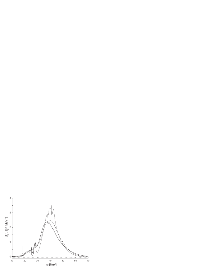
Figure 1: The “Coulomb” strength function calculated for the ²⁰⁸Pb parent nucleus within the cRPA (thin line), the semimicroscopic approach (dash–dotted line), and p–h the optical model (full line). The arrow indicates the IAR energy.

In the present work, the optical model of particle-hole-type excitations has been formulated in terms of the energy-averaged nonlocal particle-hole Green function. The equation for this Green function involves a specific energy-dependent particle-hole interaction, which is due to virtual excitation of many-quasiparticle configurations. The intensity of the imaginary part of this interaction should be taken nearly constant within nuclear volume to satisfy the statistical assumption on the independent spreading of different particle-hole-type states which form a given giant resonance. The strength function of the “single-level” giant resonance can be described in terms of the energy-averaged local particle-hole Green function.

Along with numerical realizations, the particle-hole optical model can be extended to describe direct particle decays of giant resonances. These points are under consideration.

In conclusion, one can say that in formulation of the particle-hole optical model we are on a way from fantasy to reality.

The author thanks M.L. Gorelik for the calculation leading to the results presented in Fig. 1, and I.V. Safonov for his kind help in preparing the manuscript.

This work is partially supported by RFBR under grant no. 09-02-00926-a.

References

- (1) S. Shlomo, G. Bertsch, Nucl. Phys. A 243, 507 (1975).
- (2) G.F. Bertsch, P.F. Bortignon, R.A. Broglia, Rev. Mod. Phys. 55, 287 (1983).
- (3) S. Kamerdziev, J. Speth, G. Tertychny, Phys. Rep. 393, 1 (2004).
- (4) G. Coló, N. Van Giai, P.F. Bortignon, R.A. Broglia, Phys. Rev. C 50, 1496 (1994).
- (5) M.L. Gorelik, I.V. Safonov, M.H. Urin, Phys. Rev. C 69, 054322 (2004).
- (6) M.H. Urin, Nucl. Phys. A 811, 107 (2008).
- (7) B.A. Tulupov, M.G. Urin, Phys. At. Nucl. 72, 737 (2009).
- (8) M.L. Gorelik, B.A. Tulupov, M.G. Urin, Phys. At. Nucl. 69, 598 (2006).
- (9) N. Auerbach, Phys. Rep. 98, 273 (1983)
- (10) I.V. Safonov, M.G. Urin, Bull. Rus. Acad. Sci. Phys. 67, 44 (2003).
- (11) M.L. Gorelik, V.S. Rykovanov, M.G. Urin, Bull. Rus. Acad. Sci. Phys. 73, 1551 (2009); Phys. At. Nucl. 73 (2010) (in press).
- (12) C. Mahaux, S. Sartor, Adv. Nucl. Phys. 20, 1 (1991).
- (13) M.G. Urin, “Relaxation of nuclear excitations”, Energoatomizdat, Moscow, 1991 (in Russian); S.E. Muraviev, M.G. Urin, Particles and Nuclei, 22, 882 (1991).
- (14) E.A. Romanovskii et al., Phys. At. Nucl. 63, 399 (2000); O.V. Bespalova et al., Phys. At. Nucl. 69, 796 (2006).
- (15) G.A. Chekomazov, M.H. Urin, Phys. Lett. B 349, 400 (1995); Phys. At. Nucl. 61, 375 (1998).
- (16) A.B. Migdal, “Theory of finite Fermi-sistems and applications to atomic nuclei”, Interscience, New York, 1967.
- (17) M.L. Gorelik and M.H. Urin, Phys. Rev. C 63, 064312 (2001).