Evaluating free flux flow in low-pinning molybdenum-germanium superconducting films

Abstract

Vortex dynamics in molybdenum-germanium superconducting films were found to well approximate the unpinned free limit even at low driving forces. This provided an opportunity to empirically establish the intrinsic character of free flux flow and to test in detail the validity of theories for this regime beyond the Bardeen-Stephen approximation. Our observations are in good agreement with the mean-field result of time dependent Ginzburg-Landau theory.

I Introduction and background

The motion of magnetic flux vortices in the mixed state of type II superconductors is one of the most studied aspects of superconductors. The most fundamental transport regime of the mixed state is the state of free flux flow (FFF) where the “Lorentz” force on the vortices is balanced only by the intrinsic viscous drag, without any additional interactions arising from pinning, elastic strains, thermal gradients, etc.

One of the rudimentary characteristics expected of the FFF regime (as long as $j$ is not large enough to alter the superconducting state) is that the transport response be Ohmic, so that the flux-flow chordal resistivity $\rho_{f}=E/j$, not just the differential resistivity $\rho_{d}=dE/dj$, is constant; here $E$ is the electric field and $j$ is the current density. At sufficiently low values of $B$, where each vortex behaves independently, $\rho_{f}$ is simply proportional to the number density of vortices and hence to the magnetic field $B$. In this limit, elementary theories of flux flow tinkham ; bs ; clem have shown that the proportionality factor is of the order of $\rho_{n}/H_{c2}$ resulting in the Bardeen-Stephen (BS) relation $\rho_{f}\sim\rho_{n}B/H_{c2}$, where $\rho_{n}$ is the normal-state resistivity and $H_{c2}$ is the upper critical field (we set $\mu_{0}=1$ and use units of tesla for both the magnetic field $B$ as well as the magnetizing field $H$). As $B$ is increased beyond this low-field limit, additional effects set in—such as the suppression of the order parameter with increasing $B$, changes in the circulating current patterns around the vortices, et cetera—causing the response to deviate from $\rho_{f}$ $\propto B$. More advanced theories such as the work by Larkin and Ovchinnikov lo using a microscopic Green-function approach, and various works schmid ; caroli ; vecris ; ullah ; dorsey ; troy based on time dependent Ginzburg-Landau theory, calculate the detailed $\rho_{f}(B,T)$ behavior beyond the Bardeen-Stephen approximation. These theories have not been sufficiently verified before.

While there is an impressive body of experimental work that has discovered or confirmed many interesting and exotic regimes of vortex dynamics (such as vortex glass, melting, flux creep, vortex instability, etc.) the fundamental FFF regime is the least completely studied of these. Even the expected Ohmic behavior is usually not observed with high accuracy; many previous reports obs ; gapud ; dasgupta ; lefloch ; berghuis either plot the differential ($dE/dj$) instead of the chordal ($E/j$) resistivity, and/or use logarithmic scales so that the deviation from Ohmic behavior is less conspicuous than it can be on a linear-linear plot of $\rho$ versus $j$. In some earlier work obs ; gapud ; dasgupta ; lefloch , high current densities were able to largely overcome pinning so that $\rho$ became at least roughly constant. These previous works were able to establish, at least on a coarse scale, the adherence to the basic BS behavior. There are a few partial reports berghuis ; babic-noise ; babic-instability that compare an observed $\rho_{f}(B,T)$ curve with the LO theory, but the FFF regime has not been systematically investigated so as to make a detailed evaluation of the different theories that apply to this regime.

In the present work we were able to cleanly observe FFF behavior in low-pinning molybdenum-germanium (MoGe) superconducting films, over the temperature range $0.6T_{c}\lesssim T\leq T_{c}$, with exact Ohmic behavior visible on an uncompressed linear-linear scale even for low current densities ($j/j_{d}\sim 1\times 10^{-4}$ and $j/j^{*}\sim 1\times 10^{-2}$ where $j_{d}$ and $j^{*}$ are the depairing and flux-flow-instability values respectively) that avoid non-linear alterations that can arise from high $j$. Our data allow us to empirically elucidate the character of the FFF regime and to test theories that make detailed predictions beyond Bardeen-Stephen.

All theories for free flux flow are restricted in one way or another (e.g., $T$ close to $T_{c}$, $B$ close to $H_{c2}$, gapless case, etc.). A microscopic treatment of this phenomenon, which is unrestricted in its $B/H_{c2}$ range (although restricted to $T$ close to $T_{c}$) is that due to Larkin and Ovchinnikov lo (LO) who find (their Eq. 22):

$$\sigma_{f}=\sigma_{n}+\frac{\sigma_{n}}{(1-T/T_{c})^{1/2}}\frac{H_{c2}}{B}\tilde{f}(B/H_{c2}),$$ (1)

where non-linearities that occur at higher values of $B$ are contained in the $\tilde{f}(B/H_{c2})$ function that they describe in their paper (their Table 1 and related text).

Alternatively, various authors schmid ; caroli ; vecris ; ullah ; dorsey ; troy have calculated the flux-flow conductivity using a TDGL (time dependent Ginzburg-Landau) approach. The applicable mean-field result can be written as:

$$\sigma_{f}=\sigma_{n}+\sigma_{n}\left(\frac{H_{c2}-B}{\nu B}\right),$$ (2)

where $\nu\sim 0.4$ is a roughly $T$, $B$, and material independent parameter nucalc . Despite TDGL’s strict validity for only gapless superconductivity, we find that Eq. 2 fits our observations quite well, taking $\nu$ as an adjustable parameter that we allow to be determined by the experiment.

II Experimental techniques

Films of thickness $t=50$ nm were sputtered onto silicon substrates with 200 nm thick oxide layers from a Mo_0.79Ge_0.21 alloy target. The deposition system had a base pressure of $2\times 10^{-7}$ Torr and the argon gas working pressure was maintained at 3 mTorr during the sputtering. The growth rate was 0.15 nm/s. The samples were patterned into bridges of length $l=102\ \mu$m and width $w=6\ \mu$m using photolithography and argon ion milling. Measurements were conducted on four samples A–D. Their transition temperatures $T_{c}$, normal-state resistances $R_{n}$, upper-critical-field slopes $H^{\prime}_{c2}=dH_{c2}/dT|_{T_{c}}$, corresponding $H_{c2}(0)$ values (obtained using the WHH [Werthamer, Helfand, and Hohenberg] formalism whh ), and Ginzburg-Landau (GL) parameter $\kappa=3.54\times 10^{4}\sqrt{-\rho_{n}\mu_{o}H^{\prime}_{c2}}$ (from Kes and Tsuei kes1983 ) are as follows. Sample A: $T_{c}$=5.56 K, $R_{n}$=555 $\Omega$, $H^{\prime}_{c2}$=-3.13 T/K, $H_{c2}(0)$=12.0 T, and $\kappa$=78. Sample B: $T_{c}$=5.41 K, $R_{n}$=555 $\Omega$, $H^{\prime}_{c2}$=-3.13 T/K, $H_{c2}(0)$=11.7 T, and $\kappa$=78. Sample C: $T_{c}$=5.01 K, $R_{n}$=630 $\Omega$, $H^{\prime}_{c2}$=-3.0 T/K, $H_{c2}(0)$=10.3 T, and $\kappa$=77. Sample D: $T_{c}$=5.00 K, $R_{n}$=540 $\Omega$, $H^{\prime}_{c2}$=-2.63 T/K, $H_{c2}(0)$=9.1 T, and $\kappa$=67.

The cryostat was a Cryomech PT405 pulsed-tube closed-cycle refrigerator that went down to about 3.2 K. It was fitted inside a 1.3 tesla GMW 3475-50 water-cooled copper electromagnet. Calibrated cernox and hall sensors monitored $T$ and $B$ respectively. The triggers of all measuring instruments were synchronized with the pulsed-tube compressor cycle and instrument measurement windows were set to 1 power line cycle (16.7 ms $\sim$3% of the compressor cycle) which ensured a temperature consistency of $\sim$10 mK. The main electrical resistivity measurements were made using a standard dc four-probe method with an in-house built dc current source and voltages measured with a Keithley model 2000 multimeter. Some extended IV curves were measured using 0.005 % duty cycle 20 $\mu$s duration pulses (with in-house built pulsed-current source and differential preamplifier, and a LeCroy model 9314A digital storage oscilloscope) to obtain a broader view of the behavior that includes higher currents up to and beyond the vortex instability; however, these high-$j$ measurements are not essential for the analysis and conclusions of the present work, which pertains to the low-driving force regime. All data presented here were found to be completely reversible and showed no hysteresis with respect to cycling of $I$, $B$, and $T$. Further details of the measurement techniques have been published in previous review papers pbreview ; mplb .

III Results and analysis

Fig. 1 shows some examples of mixed-state transport responses. Panel (a) shows $R$ vs $I$ curves on a linear-linear graph to best illustrate the constancy of $R$. Panel (b) shows $V$ vs $I$ curves: the absence of an intercept again emphasizes that the response is Ohmic (homogeneously linear) and not just linear with an offset. Both panels (a) and (b) were measured with continuous dc currents of values that are low compared with $j_{d}$ (by $10^{-4}$) and $j^{*}$ (by $10^{-2}$). Panel (c) shows an example of a global view of the transport response that includes the high-$j$ behavior measured using pulsed currents. As can be seen, the response becomes progressively more non-linear with rising $j$, eventually leading to an instability where the curves bend around and enter a negative sloped region: There is no reentrant Ohmic behavior (e.g., please see Fig. 2 of Ref. mplb, or Fig. 5 of Ref. blatter, ) that one often sees when the low-$j$ Ohmic region is due to thermally assisted flux flow taff (TAFF) rather than FFF. TAFF, well known from high-temperature superconductors, corresponds to the case of a weakly pinned flux liquid in the presence of large thermal activation (when the pinning energy $U_{0}\ll k_{B}T$). TAFF is characterized by an exponentially reduced resistivity (as in the case of Ref. babic-noise, where they see an approximately Ohmic response in the pinned regime at feeble current densities [10 A/cm²], albeit with a value that is 8% of $\rho_{f}$) whereas here we find $\rho_{f}$ of the same order as the nominal Bardeen-Stephen value (indeed we find rather detailed agreement with Eq. 2). When a resistive transition is characterized by TAFF, it is expected to show the Arrhenius dependence $\log R\sim-1/T$; as we show later our resistive transitions do not exhibit this behavior but instead follow the prediction of Eq. 2. This absence of TAFF behavior is consistent with MoGe’s small Ginzburg number ginzburg ; blatter of $Gi=10^{-13}\kappa^{4}T_{c}^{2}/H_{c2}(0)\sim 5\times 10^{-6}$. (In Ref. babic-noise, , in the comparable NbGe system, they observe quasi-Ohmic behavior presumably corresponding to TAFF; but their current densities are $10^{3}$ times smaller than ours.) All of the $\rho_{f}$ data that are subsequently plotted and analyzed, were checked for Ohmic behavior and constancy of $R$ as in Fig. 1(a), to ensure that the data lie in the FFF regime.

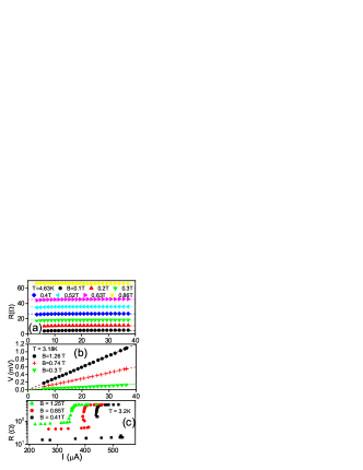
Figure 1: (a) $R$ vs $I$ curves for sample A. The horizontal lines are least-squares fits to the data. (b) $V$ vs $I$ curves for sample B. The lines are least-squares fits to the data extrapolating to the origin. (c) Extended $V$ vs $I$ curves (measured with pulsed signals) for sample D that include the vortex instability region.

Fig. 2 shows, for samples A (top row) and B (bottom row), the free-flux-flow resistances as measured above plotted against the magnetic field. The vertical scale corresponds to a normalized resistance range of $0\lesssim R/R_{n}\lesssim 0.5$. (In a later figure we show resistive transitions, which include the $R\rightarrow R_{n}$ region.) The different curves correspond to different temperatures as indicated. At low $B$ the response is linear and at higher $B$ it curves upward (the simple BS formula corresponds to a linear response for all $B$). The left column (panels (a) and (c)) shows fits to the LO theory (Eq. 1) and the right column (panels (b) and (d)) shows fits to the TDGL theory (Eq. 2). While both theories are in principle restricted to work only close to $T_{c}$, the TDGL result provides an excellent description of the observed behavior over the entire range, whereas the LO fits have shapes that do not conform to the data even for $T/T_{c}>0.9$ (top 3 curves) where they ought to work (it appears that the $\tilde{f}$ function in Eq. 1 has excessive curvature so that the LO fits can’t be much improved even with a scaling constant). Both theories show a greater departure when $R\rightarrow R_{n}$, a region that is better revealed in plots of the resistive transition shown in a later figure. For the TDGL fits (panels (b) and (d) of Fig. 2), $\nu$ was taken as a fitting parameter for each curve so that the dependence $\nu(T)$ could be determined. This procedure was repeated for the other two samples. The resulting values of $\nu(T)$ for all four samples are shown in Fig. 3(a). The observed $\nu(T)$ is relatively flat with respect to temperature with values in the 0.2–0.4 range, which are consistent with the estimate of $\nu\sim 0.4$ from theory nucalc .

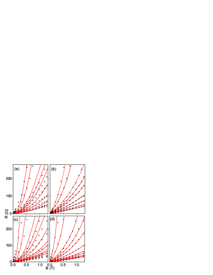
Figure 2: (a) and (b) Resistance versus magnetic field data (symbols) for sample A at temperatures (bottom to top): $T$=3.25, 3.74, 4.24, 4.56, 4.79, 4.90, 5.00, 5.21, 5.31 K. (c) and (d) Resistance versus magnetic field data (symbols) for sample B at temperatures (bottom to top): $T$ = 3.17, 3.48, 3.71, 4.01, 4.21, 4.53, 4.77, 4.88, 4.98, 5.19, 5.30 K. (a) and (c) show fits to LO theory (Eq. 1). (b) and (d) show fits to the TDGL theory (Eq. 2) using $\nu$ as a fitting parameter for each curve (i.e., for each $T$). The resulting values of $\nu$ are shown in Fig. 3. All fits use the same $H_{c2}$$(T)$ given by $H_{c2}(T)=H^{\prime}_{c2}[T-T_{c0}]$ and the measured value $H^{\prime}_{c2}$=-3.125 T/K.

In the literature, we found one comparable $R$ versus $B$ curve for another low pinning system (amorphous Nb₃Ge) by Berghuis et al. berghuis (even though they plot differential rather than the chordal resistivity, their data appear to lie approximately in the FFF regime). Their data are shown in Fig. 3(b). As can be seen, the solid red line corresponding to the TDGL function (with $\nu=0.27$) fits the entire range of their data well (this $\nu$ is shown in panel (a) as an asterisk). In their paper, the authors fit the data to the LO prediction for the $B\approx H_{c2}$ region (Eq. 30 of LO):

$$\sigma_{f}=\sigma_{n}+\sigma_{n}\tilde{\alpha}[1-B/H_{c2}]$$ (3)

with $\tilde{\alpha}=2.44$. That fit is shown as a dashed blue line in Fig. 3(b) (in their paper the authors show only the first-order linear expansion $\rho_{f}/\rho_{n}\approx 1-\tilde{\alpha}[1-B/H_{c2}]$ of Eq. 3). On the same plot we have also shown a curve corresponding to Eq. 1 (the LO prediction for $T\approx T_{c}$, since these data correspond to $T/T_{c}=0.85$) as the black dotted line. As can be seen, both LO curves show marginal agreement with the data and only over a very narrow range.

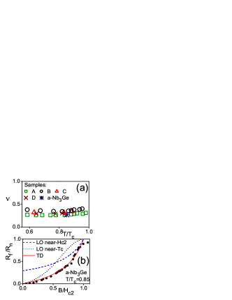
Figure 3: (a) Experimentally deduced parameter $\nu$ (of Eq. 2) and its variation with temperature for MoGe samples A–D. The asterisk shows a $\nu$ value for the Nb₃Ge data of reference berghuis, plotted in panel (b). (b) Normalized resistance versus normalized field for amorphous Nb₃Ge films from Berghuis et al. berghuis . $t=T/T_{c}=0.85$ with $T_{c}$=2.93 K. Solid red line represents a TDGL curve (Eq. 2) with $\nu$=0.27. Blue dashed and black dotted lines correspond to the LO theory for the condition “close to $H_{c2}$” (Eq. 3) with $\tilde{\alpha}$=2.44 and for the condition “close to $T_{c}$”(Eq. 1) respectively.

To explore the region close to $T\approx T_{c}$ and $R_{f}\approx R_{n}$, we show in Fig. 4 the resistive transitions in various magnetic fields. Panel (a) shows the data for sample A along with LO curves (Eq. 1); there is some resemblance in trends between the data and theory, but for the most part the agreement is not close. Panels (b) and (d) show the data for samples A and B along with TDGL curves (Eq. 2). Given our earlier empirical confirmation that $\nu$ is $T$ independent (Fig. 3(a)), we tried to fit all curves for each sample with a single $\nu$ value. As can be seen, for each of panels (b) and (d), the TDGL theory provides excellent agreement with the observed behavior over the lower and middle portion of the $R_{f}/R_{n}$ range with a single parameter. The obtained values of $\nu=$ 0.34, 0.26, 0.23, and 0.31 (for samples A–D respectively) are quantitatively consistent with the theoretically estimated $\nu\sim 0.4$. The region right around the transition does not fit either theory well, perhaps because of a cross over to 2 dimensionality babic-noise or additional effects kogan-zhelezina not included in the present theories, as well as because of the finite width of the transition. Panel (c) plots the data for sample A as log $R$ versus $1/T$. As can be seen it does not exhibit the Arrhenius behavior ($R\propto e^{-1/T}$) that characterizes the TAFF regime.

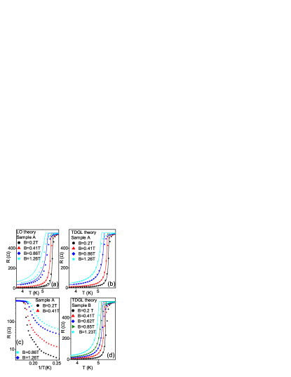
Figure 4: Resistive transitions in magnetic fields. Symbols show experimental data. Solid lines are theoretical curves. (a) Sample A with LO theory curves (Eq. 1). (b) Sample A with TDGL theory curves (Eq. 2 with $\nu$=0.34 for all $B$ and $T$). (c) Arrhenius plots of the same resistive-transition data for Sample A. (d) Sample B with TDGL theory curves (Eq. 2 with $\nu$=0.26 for all $B$ and $T$).

IV Summary and conclusions

Free flux flow is the most primitive regime of transport in the mixed state; however, its experimental investigation is normally hindered by gross alterations of the dynamics due to pinning and other complications (dissociation into pancakes due to a layered structure, exotic gap symmetries, melting/entanglement due to high temperatures, etc.). The present experiment has observed clean FFF behavior in one of the simplest and nearly model superconductors (unpinned, isotropic, low-temperature, weak-coupling BCS, etc.). This allowed us to look closely at the transport characteristics of this regime beyond the simple Bardeen-Stephen formula $\rho_{f}\sim\rho_{n}B/H_{c2}$ and to assess the applicability and accuracy of the microscopic and TDGL theories. We find that the mean-field result arising out of TDGL provides a much better agreement with the observed $\rho_{f}(B,T)$ function—and is applicable over a wider range of conditions—than the theory of Larkin and Ovchinnikov.

Besides the one experimental curve from Ref. berghuis, (shown in our Fig. 3(b)) where the authors apply the near-$H_{c2}$ LO $\rho_{f}(B,T)$ function (Eq. 3, shown as the blue dashed line in Fig. 3(b)), in the works by Babic et al. on vortex noise babic-noise and vortex instability babic-instability , the authors show (incidentally to the main investigations of those papers) partial agreement with the near-$T_{c}$ LO $\rho_{f}(B,T)$ function (Eq. 1); the insets of their Figs. 1 of both Ref. babic-noise, and Ref. babic-instability, each show one experimental curve for one temperature for one sample.

The present work only evaluates the accuracy of the $\rho_{f}(B,T)$ function in the FFF regime and makes no comments on the accuracy and applicability of the LO theory for other regimes such as the vortex instability. An important value of a microscopic theory such as LO lies in its ability to go beyond phenomenology and make a connection between measurements and microscopic parameters (such as the extraction of the inelastic scattering time as carried out in Ref. berghuis, ).

On the other hand, the mean-field result of the TDGL theory provides a rather excellent account of the observed $\rho_{f}(B,T)$ function as seen from Figs. 2 and 4 along with quantitative agreement with the predicted parameter $\nu$. This is a useful observation, because in some calculations of exotic effects—such as vortex instabilities—the BS formula is often used as a starting point. For such applications, the TDGL formula (Eq. 2) with $\nu\sim$ 0.2–0.4 may provide a more accurate alternative while retaining most of the simplicity of the BS result.

V Acknowledgements

The authors gratefully acknowledge useful discussions with James M. Knight, Alan T. Dorsey, Boris I. Ivlev, Alexander V. Gurevich, Vladimir G. Kogan, Lev Bulaevski, David K. Christen, Ernst Helmut Brandt, and P. H. Kes. This work was supported by the U. S. Department of Energy through grant number DE-FG02-99ER45763. The sample fabrication work at Northern Illinois University was supported by the U.S. Department of Energy through grant number DE-FG02-06ER46334.

References

- (1) M. Tinkham, Phys. Rev. Lett. 13, 804 (1964).
- (2) J. Bardeen and M. J. Stephen, Phys. Rev. 140, A1197 (1965).
- (3) J. R. Clem, Phys. Rev. Lett. 20, 735 (1968).
- (4) A. I. Larkin and Yu. N. Ovchinnikov, in Nonequilibrium Superconductivity, D. N. Langenberg and A. I. Larkin, eds. (Elsevier, Amsterdam, 1986), Ch. 11.
- (5) A. Schmid, Phys. Kondens. Mater. 5, 301 (1966).
- (6) C. Caroli and K. Maki, Phys. Rev. 164, 591. (1967).
- (7) G. Vecris and R. A. Pelcovits, Phys. Rev. B44, 2767 (1991).
- (8) S. Ullah and A. T. Dorsey, Phys. Rev. B44, 262 (1991).
- (9) A. T. Dorsey, Phys. Rev. B46, 8376 (1992).
- (10) R. J. Troy and A. T. Dorsey, Phys. Rev. B 47, 2715 (1993).
- (11) M. N. Kunchur, D. K. Christen, and J. M. Phillips, Phys. Rev. Lett. 70, 998 (1993).
- (12) A. A. Gapud, S. Moraes, R. P. Khadka, P. Favreau, C. Henderson, P. C. Canfield, V. G. Kogan, A. P. Reyes, L. L. Lumata, D. K. Christen, and J. R. Thompson, Phys. Rev. B 80, 134524 (2009).
- (13) K. Das Gupta, S. S. Soman, N. Chandrasekhar, Physica C 388–389, 771 (2003).
- (14) F. Lefloch, C. Hoffmann, and O. Demolliens, Physica C 319, 258 (1999).
- (15) P. Berghuis, A. L. F. van der Slot, and P. H. Kes, Phys. Rev. Lett. 65, 2583 (1990).
- (16) D. Babic, T. Nussbaumer,C. Strunk, C. Schonenberger, and C. Surgers, Phys. Rev. B 66, 014537 (2002).
- (17) D. Babic, J. Bentner, C. Surgers, and C. Strunk, Phys. Rev. B 69, 092510 (2004).
- (18) In SI units, the expression for can be written as (for ); here is the real part of the dimensionless order-parameter relaxation time and =1.16 for a triangular flux lattice. As per Fukuyama, Ebisawa, and Tsuzuki fukuyama , . With the substitutions gorkov1959 ; kes1983 and we get . Note that to first order, is independent of , , and material parameters.
- (19) N. R. Werthamer, E. Helfand, and P. C. Hohenberg, Phys. Rev. 147, 295 (1966); and E. Helfand and N. R. Werthamer, Phys. Rev. 147, 288 (1966).
- (20) P. H. Kes and C. C. Tsuei, Phys. Rev. B28, 5126 (1983).
- (21) M. N. Kunchur, Mod. Phys. Lett. B 9, 399 (1995).
- (22) M. N. Kunchur, J. Phys.: Condens. Matter 16, R1183-R1204 (2004).
- (23) G. Blatter, M. V. Feigel’man, V. B. Geshkenbein, A. I. Larkin, V. M. Vinokur, Rev. Mod. Phys. 66, 1125 (1994).
- (24) P. H. Kes, J. Aarts, J. van den Berg, C. J. van der Beek, and J. A. Mydosh, Supercond. Sci. Technol. 1, 242 (1989).
- (25) V. L. Ginzburg, Fiz. Tverd. Tela 2, 2031 (1960) [Sov. Phys. Solid State 2, 1824 (1961)].
- (26) V. G. Kogan and N. V. Zhelezina, Phys. Rev. B 71, 134505 (2005).
- (27) H. Fukuyama, H. Ebisawa, and T. Tsuzuki, Prog. Theor. Phys. 46, 1028 (1971).
- (28) L. P. Gorkov, Zh. Eksp. Teor. Fiz. 36, 1918 (1959) [Sov. Phys.—JETP 9, 1364 (1959); L. P. Gorkov, Zh. Eksp. Teor. Fiz. 37, 1407 (1959) [Sov. Phys.—JETP 10, 998 (1960)].