Evaluation of pressure boundary conditions for permeability calculations using the lattice-Boltzmann method

Abstract

Lattice-Boltzmann (LB) simulations are a common tool to numerically estimate the permeability of porous media. For valuable results, the porous structure has to be well resolved resulting in a large computational effort as well as high memory demands. In order to estimate the permeability of realistic samples, it is of importance to not only implement very efficient codes, but also to choose the most appropriate simulation setup to achieve accurate results. With the focus on accuracy and computational effort, we present a comparison between different methods to apply an effective pressure gradient, efficient boundary conditions, as well as two LB implementations based on pore-matrix and pore-list data structures.

1 Introduction

The lattice-Boltzmann (LB) method is a numerical scheme that is able to simulate the hydrodynamics of fluids with complex interfacial dynamics and boundaries bib:mcnamara-zanetti ; bib:higuera-succi-benzi ; bib:chen-chen-matthaeus ; bib:qian-dhumieres-lallemand ; bib:chen-chen-martinez-matthaeus ; bib:succi-01 . Its popularity stems from the broad field of possible application and a fair implementation effort compared to other CFD methods. Unlike schemes that are based on a discretization of the Navier-Stokes equations, and therefore represent balance equations at the continuum level (macroscopic), the LB method represents the dynamics at mesoscopic level by solving the discretized Boltzmann equation.

There is an increasing interest in the LB method for simulation of flow in complex geometries since the end of the 1980’s citeulike:3986220 when hydrodynamic simulation methods were dominated by finite element schemes that solved the Stokes equation PhysRevB.46.6080 ; 1996AREPS..24…63V . With the advent of more powerful computers it became possible to perform detailed simulations of flow in artificially generated geometries koponen:3319 , tomographic reconstructions of sandstone samples bib:ferreol-rothman ; Martys99largescale ; MAKHT02 ; bib:jens-venturoli-coveney:2004 ; Ahren06 , or fibrous sheets of paper koponen:716 . An important property estimated using the LB method in those geometries is the permeability bib:darcy , and since the porous structure has to be well resolved in order to obtain valuable results, a large computational effort as well as high memory demands is required. Therefore, it is important to develop very efficient simulation paradigms.

Different alternative simulation setups have been proposed for permeability estimation which differ in the computational domain setup, how the fluid is driven, or how an effective pressure gradient is being estimated. Further possible differences include the choice between single relaxation and multirelaxation time lattice Boltzmann implementations or data structures based on a 3D array containing the whole discretized simulation volume including rock matrix and pore space (pore-matrix) in contrast to data structures limited to a connected list of pore nodes (pore-list) bib:succi-01 ; 2005ASIM:DXHHW .

The current paper focuses on a detailed comparison of some of these possible implementation details to accurately estimate the permeability of porous media with the LB method. We compare the well known D3Q19 single relaxation (LB-BGK) bib:bgk ; bib:chen-chen-martinez-matthaeus and multirelaxation time (LB-MRT) 2002RSPTA.360..437D models together with three alternative setups to estimate the permeability utilizing an injection channel of variable length (I-Ch), pressure boundary conditions ($p$-BC), or a force density applied over the sample ($\nabla p$-S). The geometries being investigated are a 3D Poiseuille flow in a square pipe and a BCC sphere array. While the first one has the advantage of a minimal discretization error, the second one more realistically resembles a natural porous medium. We also present a comparison of the efficiency of the LB-codes based on the above mentioned pore-matrix and pore-list data structures 2005ASIM:DXHHW .

2 The Lattice-Boltzmann Method

Figure 1: D3Q19 cubic lattice with lattice vectors $\mathbf{c}_{\dot{\imath}}$.

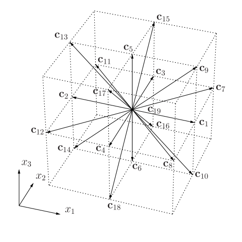
The discretized lattice-Boltzmann (LB) equation reads

$$n_{\dot{\imath}}(\mathbf{x}+\mathbf{c}_{\dot{\imath}}\Delta t,t+\Delta t)-n_{\dot{\imath}}(\mathbf{x},t)=\Delta t\sum_{\dot{\jmath}=1}^{N}S_{\dot{\imath}\,\dot{\jmath}}\left(n_{\dot{\jmath}}(\mathbf{x},t)-n^{\mathrm{\tiny{eq}}}_{\dot{\jmath}}(\mathbf{x},t)\right),$$ (1)

where $\mathbf{x}=(x_{1},x_{AJ},x_{3})$ represents a node. The discretization parameters are $\Delta t$ and $\Delta x$, while the discrete velocities $\mathbf{c}_{\dot{\imath}}$ have the dimension $\Delta x/\Delta t$. The variable $n_{\dot{\imath}}$ is the probable number of particles moving with velocity $\mathbf{c}_{\dot{\imath}}$. We use a 3D cubic lattice with 19 discrete velocities $\mathbf{c}_{\dot{\imath}},\,\dot{\imath}=1\ldots 19$ known as D3Q19 (see Fig. 1 for a visualization) bib:qian-dhumieres-lallemand . The term on the right hand side of Eq. (1) is the linearized collision operator, where $S_{\dot{\imath}\,\dot{\jmath}}$ is the collision matrix also known as scattering matrix and $n^{\mathrm{\tiny{eq}}}_{\dot{\jmath}}(\mathbf{x},t)$ is the equilibrium distribution bib:higuera-succi-benzi . The macroscopic density $\rho(\mathbf{x},t)$ and velocity $\mathbf{u}(\mathbf{x},t)$ are obtained from $n_{\dot{\imath}}(\mathbf{x},t)$ as

$$\rho(\mathbf{x},t) = \rho^{\circ}\sum_{\dot{\imath}=1}^{N}n_{\dot{\imath}}(\mathbf{x},t),$$ (2)

$$\rho(\mathbf{x},t)\mathbf{u}(\mathbf{x},t) = \rho^{\circ}\sum_{\dot{\imath}=1}^{N}n_{\dot{\imath}}(\mathbf{x},t)\,\mathbf{c}_{\dot{\imath}},$$ (3)

where $\rho^{\circ}$ is a reference density. The pressure is given by

$$p(\mathbf{x},t)={c_{\mathrm{s}}}^{2}\,\rho(\mathbf{x},t),$$ (4)

with

$${c_{\mathrm{s}}}=\frac{1}{\sqrt{3}}\left(\frac{\Delta x}{\Delta t}\right)$$ (5)

being the speed of sound bib:qian-dhumieres-lallemand . The kinematic viscosity $\nu$ is defined as

$$\nu=\frac{{c_{\mathrm{s}}}^{2}\Delta t}{2}\left(2\frac{\tau}{\Delta t}-1\right).$$ (6)

Within the LB method, the single relaxation time (BGK) or multirelaxation time (MRT) methods differ only in the way how the terms $S_{\dot{\imath}\,\dot{\jmath}}$ and $n^{\mathrm{\tiny{eq}}}_{\dot{\jmath}}(\mathbf{x},t)$ are defined. In the case of the LB-BGK scheme bib:bgk ; bib:chen-chen-martinez-matthaeus , the matrix $S_{i\,j}=-\delta_{\dot{\imath}\,\dot{\jmath}}/\tau$, where $\tau$ is a unique relaxation time and $\delta_{\dot{\imath}\,\dot{\jmath}}$ is the Kroneker delta. The equilibrium distributions

$$n^{\mathrm{\tiny{eq}}}_{\dot{\imath}}(\mathbf{x},t)=\omega_{\text{\tiny{$\mathbf{c}_{\dot{\imath}}$}}}\frac{\rho}{\rho^{\circ}}\left(1+\frac{\mathbf{u}^{*}\cdot\mathbf{c}_{\dot{\imath}}}{{c_{\mathrm{s}}}^{2}}+\frac{(\mathbf{u}^{*}\cdot\mathbf{c}_{\dot{\imath}})^{2}}{2{c_{\mathrm{s}}}^{4}}-\frac{\mathbf{u}^{*}\cdot\mathbf{u}^{*}}{2{c_{\mathrm{s}}}^{2}}\right),$$ (7)

are obtained from a 2${}^{\text{nd}}$ order Taylor approximation of the Maxwell distribution function bib:DHae:04 , with $\mathbf{u}^{*}=\mathbf{u}^{*}(\mathbf{x},t)$ and $\rho=\rho(\mathbf{x},t)$ calculated in absence of an external force as $\mathbf{u}^{*}(\mathbf{x},t)=\mathbf{u}(\mathbf{x},t)$ using Eqs. (2) and (3). The numbers $\omega_{\text{\tiny{$\mathbf{c}_{\dot{\imath}}$}}}$ are called lattice weights and for the D3Q19 lattice they are

$$\omega_{\text{\tiny{$\mathbf{c}_{\dot{\imath}}$}}}\begin{cases}1/3,&\text{for }\mathbf{c}_{\dot{\imath}}=\mathbf{0},\\ 1/18,&\text{for }|\mathbf{c}_{\dot{\imath}}|=1,\\ 1/36,&\text{for }|\mathbf{c}_{\dot{\imath}}|=\sqrt{2}.\end{cases}$$ (8)

Generally, they depend on the lattice type, dimensions of space and on the number of discrete velocities $N$. In the article of Qian et al. bib:qian-dhumieres-lallemand a comprehensive overview on different lattices is given.

In the case of the LB-MRT scheme 2002RSPTA.360..437D the linearized collision operator is rewritten as

$$\sum_{\dot{\jmath}=1}^{N}S_{\dot{\imath}\,\dot{\jmath}}\left(n_{\dot{\jmath}}(\mathbf{x},t)-n^{\mathrm{\tiny{eq}}}_{\dot{\jmath}}(\mathbf{x},t)\right)=-{\mathbf{M}}^{-1}\cdot\mathbf{\check{S}}\cdot\left(\mathbf{m}(\mathbf{x},t)-{\mathbf{m}}^{\mathrm{\tiny{eq}}}(\mathbf{x},t)\right),$$ (9)

i.e., it is implemented in the space of the hydraulic modes of the problem $\mathbf{m}(\mathbf{x},t)=\mathbf{M}\cdot\mathbf{n}(\mathbf{x},t)$ instead of the space of the discrete velocities, where $\mathbf{M}$ is the transformation matrix. Some modes have a hydrodynamic meaning, but some of them do not and are used to improve the numerical stability as described in 2000PhRvE..61.6546L ; 2002RSPTA.360..437D . The relaxation parameters of the modes are given in the diagonal matrix $\mathbf{\check{S}}$. Only two values of the diagonal elements of $\mathbf{\check{S}}$ are used to specify the kinematic viscosity, Eq. (6), and the bulk viscosity. These are labeled $\tau$ and ${\tau_{\mathrm{bulk}}}$, respectively. In summary,

$$\mathbf{\check{S}}=\mathrm{diag}(0,1/{\tau_{\mathrm{bulk}}},1.4,0,1.2,0,1.2,0,1.2,1/\tau,\\ 1.4,1/\tau,1.4,1/\tau,1/\tau,1/\tau,1.98,1.98,1.98),$$ (10)

is assumed for the MRT method. The other values of the diagonal elements are chosen to optimize the performance of the algorithm as described in 2000PhRvE..61.6546L ; 2002RSPTA.360..437D . The components of the equilibrium distribution ${\mathbf{m}}^{\mathrm{\tiny{eq}}}(\mathbf{x},t)$, which represent the density and momentum are conserved after collision. The remaining ones are assumed to be functions of the conserved moments and for D3Q19 are explicitly given in 2002RSPTA.360..437D .

3 Driving the fluid

3.1 External force in the LB method

An external force density of the fluid $\mathbf{b}(\mathbf{x},t)$ is implemented by adding a term

$$\varphi_{\dot{\imath}}(\mathbf{x},t)=\omega_{\text{\tiny{$\mathbf{c}_{\dot{\imath}}$}}}\frac{\Delta t}{{\rho^{\circ}{c_{\mathrm{s}}}}^{2}}\mathbf{b}(\mathbf{x},t)\cdot\mathbf{c}_{\dot{\imath}}$$ (11)

to the right hand side of Eq. (1). The equilibrium velocity $\mathbf{u}^{*}(\mathbf{x},t)$ is then calculated using

$$\rho(\mathbf{x},t)\mathbf{u}^{*}(\mathbf{x},t)=\rho^{\circ}\sum_{\dot{\imath}=1}^{N}n_{\dot{\imath}}(\mathbf{x},t)\,\mathbf{c}_{\dot{\imath}},$$ (12)

but the macroscopic velocity $\mathbf{u}(\mathbf{x},t)$ has to be redefined as

$$\rho(\mathbf{x},t)\mathbf{u}(\mathbf{x},t)=\rho^{\circ}\sum_{\dot{\imath}=1}^{N}n_{\dot{\imath}}(\mathbf{x},t)\,\mathbf{c}_{\dot{\imath}}+\frac{\Delta t}{2}\mathbf{b}(\mathbf{x},t).$$ (13)

An important point to stress here is that this implementation is just a simplified alternative to add an external acceleration, recovering correctly the hydrodynamic macroscopic fields with less computational cost PhysRevE.65.046308 . In all simulations presented in this work the force density acts towards the direction of the $x_{3}$-axis, $\mathbf{b}=b\mathbf{e}_{3}$.

3.2 On-site Pressure Boundary Condition

Pressure boundary conditions can be implemented as introduced by Zou and He bib:pf.QZoXHe.1997 ; HH08b . Due to the ideal gas equation of state setting the pressure on a specific node is equivalent to setting the density, see Eq. (4). The on-site pressure BC are used to drive the flow by setting constant densities $\rho^{\mathrm{\tiny{in}}}$ and $\rho^{\mathrm{\tiny{out}}}$ ($\rho^{\mathrm{\tiny{in}}}>\rho^{\mathrm{\tiny{out}}}$) at the inlet $\mathcal{C}(1)$ and outlet $\mathcal{C}(X_{3})$ planes, i.e. the first and last plane in the direction of the flow, respectively. Expanding the calculation of the density $\rho$, Eq. (2), and momentum $\rho\mathbf{u}$, Eq. (3), leads to

$$\frac{\rho}{\rho^{\circ}} = n_{1}+n_{2}+n_{3}+n_{4}+n_{5}+n_{6}+n_{7}+n_{8}+n_{9}+n_{10}+n_{11}+$$ (14)

$$\quad+n_{12}+n_{13}+n_{14}+n_{15}+n_{16}+n_{17}+n_{18}+n_{19},$$

$$\frac{\rho}{\rho^{\circ}}\mathrm{u}_{x_{1}} = n_{1}-n_{2}+n_{7}+n_{8}+n_{9}+n_{10}-n_{11}-n_{12}-n_{13}-n_{14},$$ (15)

$$\frac{\rho}{\rho^{\circ}}\mathrm{u}_{x_{AJ}} = n_{3}-n_{4}+n_{7}-n_{8}+n_{11}-n_{12}+n_{15}+n_{16}-n_{17}-n_{18},$$ (16)

$$\frac{\rho}{\rho^{\circ}}\mathrm{u}_{x_{3}} = n_{5}-n_{6}+n_{9}-n_{10}+n_{13}-n_{14}+n_{15}-n_{16}+n_{17}-n_{18}.$$ (17)

Out of the four macroscopic values $\rho$ and $\mathbf{u}$ ($\mathrm{u}_{x_{1}}$, $\mathrm{u}_{x_{AJ}}$, and $\mathrm{u}_{x_{3}}$), only three are independent and can be set, because they have to fulfill the mass balance equation. For the calculations performed for this work, the components of the velocity $\mathrm{u}_{x_{1}}=0$ and $\mathrm{u}_{x_{AJ}}=0$ are being set, resulting in a flow perpendicular to the inlet and outlet plane. The variables $n_{5}$, $n_{9}$, $n_{13}$, $n_{15}$, and $n_{17}$ at the plane $\mathcal{C}(1)$, and $n_{6}$, $n_{10}$, $n_{14}$, $n_{16}$, and $n_{18}$ at the plane $\mathcal{C}(X_{3})$ (the first ones and last ones with positive and negative component in $x_{3}$ direction, respectively, see Fig. 1), are not being updated by the streaming step within the LB algorithm but they have to be solved in order to obtain the requested density (pressure) and velocity on the node. As it is explained above, since $\rho$, $\mathrm{u}_{x_{1}}$, and $\mathrm{u}_{x_{AJ}}$ are already set, it is not possible to also set the velocity $\mathrm{u}_{x_{3}}$, and its value has to be solved for on every node in the inlet plane $\mathcal{C}(1)$ and outlet plane $\mathcal{C}(X_{3})$. Therefore, we have a linear system of four equations and six unknowns to be solved. To complete the system of equations, bounce-back BC are assumed for the non-equilibrium part of the distribution $n_{\dot{\imath}}$ bib:pf.QZoXHe.1997

$$\begin{split}n_{5}-n^{\mathrm{\tiny{eq}}}_{5}&=n_{6}-n^{\mathrm{\tiny{eq}}}_{6},\\ n_{9}-n^{\mathrm{\tiny{eq}}}_{9}&=n_{14}-n^{\mathrm{\tiny{eq}}}_{14}-N_{x_{1}}^{x_{3}},\quad n_{13}-n^{\mathrm{\tiny{eq}}}_{13}=n_{10}-n^{\mathrm{\tiny{eq}}}_{10}+N_{x_{1}}^{x_{3}},\\ n_{15}-n^{\mathrm{\tiny{eq}}}_{15}&=n_{18}-n^{\mathrm{\tiny{eq}}}_{18}-N_{x_{AJ}}^{x_{3}},\quad n_{17}-n^{\mathrm{\tiny{eq}}}_{17}=n_{16}-n^{\mathrm{\tiny{eq}}}_{16}+N_{x_{AJ}}^{x_{3}},\end{split}$$ (18)

where the terms $N_{x_{1}}^{x_{3}}$ and $N_{x_{AJ}}^{x_{3}}$ are the transversal momentum corrections on the $x_{3}$-boundary for the distributions propagating in $x_{1}$ and $x_{AJ}$, respectively HH08b . Eq. (18) then reads

$$\begin{split}n_{5}-n_{6}&=\frac{\rho}{3\rho^{\circ}}\mathrm{u}_{x_{3}},\\ n_{9}-n_{14}&=\frac{\rho}{6\rho^{\circ}}\mathrm{u}_{x_{3}}-N_{x_{1}}^{x_{3}},\quad n_{13}-n_{10}=\frac{\rho}{6\rho^{\circ}}\mathrm{u}_{x_{3}}+N_{x_{1}}^{x_{3}},\\ n_{15}-n_{18}&=\frac{\rho}{6\rho^{\circ}}\mathrm{u}_{x_{3}}-N_{x_{AJ}}^{x_{3}},\quad n_{17}-n_{16}=\frac{\rho}{6\rho^{\circ}}\mathrm{u}_{x_{3}}+N_{x_{AJ}}^{x_{3}}.\end{split}$$ (19)

The on-site pressure BC presented by Kutay et al. Kutay2006381 uses the same equations presented here, but lacks the transversal momentum corrections $N_{x_{1}}^{x_{3}}$ and $N_{x_{AJ}}^{x_{3}}$. These terms are important when velocity gradients are present bib:pf.QZoXHe.1997 .

4 Simulation Setup

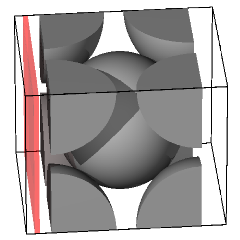
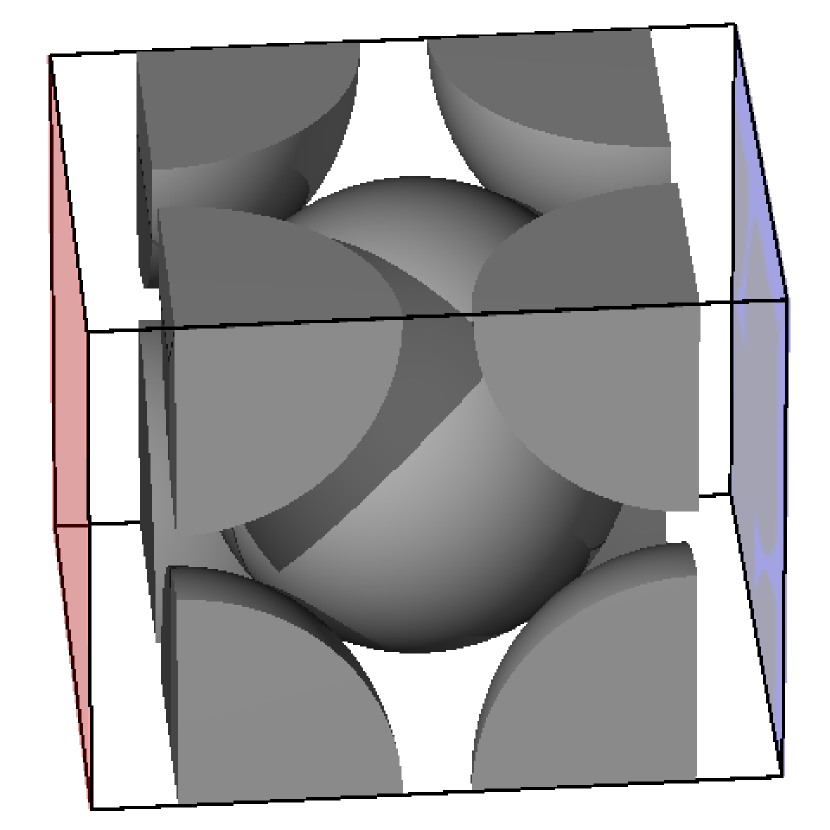
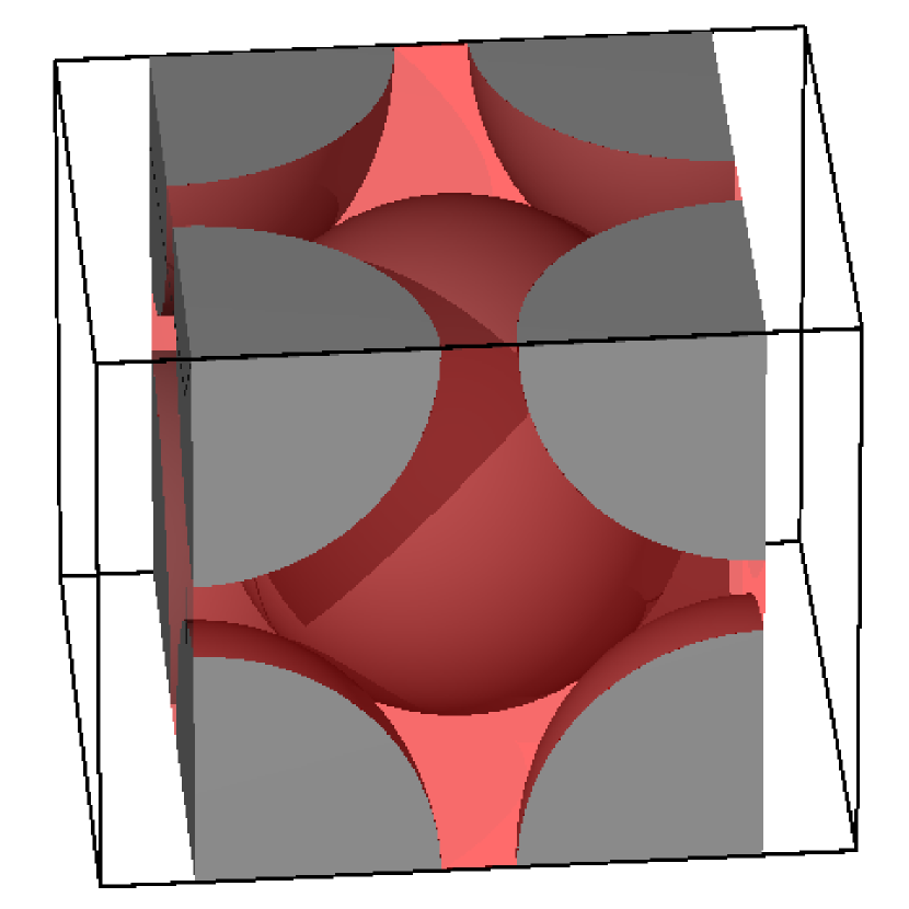
The computational domain $\mathcal{X}$ is composed of two subsets: $\mathcal{M}$ represents the solid nodes and $\mathcal{P}$ represents the fluid nodes, with $\mathcal{M}\cup\mathcal{P}=\mathcal{X}$ and $\mathcal{M}\cap\mathcal{P}=\emptyset$. The computational domain $\mathcal{X}$ with the dimensions $[X_{1}\times X_{AJ}\times X_{3}]$, has three zones as presented in Fig. 2: the inlet $\mathcal{I}$, the sample $\mathcal{S}$, and the outlet $\mathcal{O}$ with lengths $X_{\mathcal{I}}$, $X_{\mathcal{S}}$, and $X_{\mathcal{O}}$, respectively. In the case of using an injection channel the force density $\mathbf{b}$ drives the fluid in some interval of $x_{3}$ within the inlet zone $\mathcal{I}$.

Figure 2: Computational domain $\mathcal{X}$: sample $\mathcal{S}$ and two chambers $\mathcal{I}$ and $\mathcal{O}$. Cross-sections $\mathcal{C}$ are perpendicular to the direction of the flow.

Cross-sections perpendicular to the direction of flow are denoted by

$$\mathcal{C}(a)=\{\mathbf{x}\in\mathcal{X}:x_{3}=a\}.$$ (20)

For instance, the cross-sections $\mathcal{C}(X_{\mathcal{I}}+1)$ and $\mathcal{C}(X_{3}-X_{\mathcal{O}})$ represent the first and last cross-sections within the sample, respectively. The average density in the cross-section $\mathcal{C}(a)$ is calculated by

$$\langle{\rho}\rangle_{\mathcal{C}(a)}=\displaystyle{\frac{{\displaystyle{\sum_{\mathbf{x}\in(\mathcal{C}(a)\cap\mathcal{P})}\rho(\mathbf{x})}}}{{\displaystyle{\sum_{\mathbf{x}\in(\mathcal{C}(a)\cap\mathcal{P})}1}}}}.$$ (21)

The average mass flux through the whole sample is given by

$$Q=\displaystyle{\frac{{\displaystyle{1}}}{{\displaystyle{X_{3}}}}}\sum_{\mathbf{x}\in\mathcal{P}}\rho(\mathbf{x})\,\mathrm{u}_{x_{3}}(\mathbf{x})(\Delta x)^{2},$$ (22)

where $\rho(\mathbf{x})\mathrm{u}_{x_{3}}(\mathbf{x})$ is the momentum component in direction of the flow. The permeability $\kappa$ as defined by Darcy’s law is

$$\kappa=-\nu\frac{Q}{A\,\langle{(\nabla p)_{x_{3}}}\rangle},$$ (23)

where $A$ represents the cross sectional area bib:darcy . The average pressure gradient in flow direction $\langle{(\nabla p)_{x_{3}}}\rangle$ is calculated in different manners according to the way how the fluid is driven. This issue is explained in more detail below.

5 Pore-Matrix and Pore-List

The LB method is typically implemented representing the pore space and the solid nodes using a 3D array including the distribution functions $n_{\dot{\imath}}$ and a Boolean variable to distinguish between a pore and a matrix node. This 3D array is known as pore-matrix. During a simulation, at every time step the loop covering the domain includes the fluid and the solid nodes. Therefore, if-statements are necessary to distinguish whether the node represents a solid node or a fluid node where the collision and streaming steps need to be applied. Furthermore, it has to be determined for every node if BC (periodic and no-slip) need to be applied. The advantage of this data structure is its straightforward implementation. However, for the simulation of fluid flow in porous media with low porosity the drawbacks are high memory demands and inefficient loops through the whole simulation domain.

An alternative data structure, known as pore-list 2005ASIM:DXHHW , uses a two-dimensional array characterizing the porous structure. It contains the position (pore-position-list) and connectivity (pore-neighbor-list) of the fluid nodes only. It can be generated from the original 3D array before the first time step of the simulation, so that only loops through the list of pore nodes not comprising any if-statements for the lattice Boltzmann algorithm are required. The time needed to generate and save the pore-list data is comparable to the computational time required for one time step of the LB numerical scheme implemented by the pore-matrix. This alternative approach is slightly more complicated to implement, but allows highly efficient simulations of flows in geometries with a low porosity. If the porosity becomes too large, however, the additional overhead due to the connection matrix reduces the benefits and at some point renders the method less efficient than a standard implementation.

In Tbl. 1 the amount of memory required for both LB implementations is presented. Introducing the notation $F$ as the number of fluid nodes and $X^{3}=X_{1}\,X_{AJ}\,X_{3}$ as the total number of nodes, we can estimate if the pore-list implementation saves memory space using the inequality

$$(32\mathrm{bit})X^{3}+19(64\mathrm{bit})X^{3}+19(64\mathrm{bit})X^{2}\geq 3(32\mathrm{bit})F+18(32\mathrm{bit})F+38(64\mathrm{bit})F.$$ (24)

The terms on the left hand side represent the necessary memory for the pore-matrix implementation: pore-matrix, distribution function $n_{\dot{\imath}}$, and its buffer, respectively. The terms on the right hand side represent the necessary memory for the pore-list implementation: pore-position-list, pore-neighbor-list, distribution function $n_{\dot{\imath}}$, and its buffer, respectively. Neglecting the term representing the $n_{\dot{\imath}}$-buffer of the pore-matrix implementation, because of being order $X^{2}$, we can estimate that the pore-list implementation saves memory when $F/X^{3}\lesssim 0.40$, where $F/X^{3}=\phi$ is the porosity of the porous medium.

Memory Space
	Pore-Matrix	Pore-List
Geometry:	Pore-Matrix, integer $[X_{1},X_{AJ},X_{3}]$	Pore Position-List, integer $[F,3]$
		Pore Neighbor-List, integer $[F,18]$
$n_{\dot{\imath}}$:	double-precision $[X_{1},X_{AJ},X_{3},19]$	double-precision $[F,19]$
$n_{\dot{\imath}}$ buffer:	double-precision $[X_{1},X_{AJ},3,19]$	double-precision $[F,19]$

Table 1: Memory demand of implementations using a pore-matrix or a pore-list data structure. $F$ represents the number of fluid nodes.

6 Computational Domain & Setup

For the simulations six different lengths of the chambers $\mathcal{I}$ and $\mathcal{O}$, $X_{\mathcal{I}}$ and $X_{\mathcal{O}}$ are used (see Fig. 2). We restrict ourselves to $X_{\mathcal{I}}=X_{\mathcal{O}}$ and use the lengths 20, 10, 5, 2, 1 and 0. A length of 0 represents simulations without chambers. To drive the flow in order to generate an effective pressure gradient, we use three different methods:

Injection Channel (I-Ch):

In the cross-sections $\mathcal{C}(X_{\mathcal{I}}-3)$, $\mathcal{C}(X_{\mathcal{I}}-2)$, and $\mathcal{C}(X_{\mathcal{I}}-1)$ a constant force density $b\,(\Delta t)^{2}/(\rho^{\circ}\,\Delta x)=10^{-5}$ is applied and periodic BC act in all directions. The pressure gradient is estimated using

$$\langle{(\nabla p)_{x_{3}}}\rangle={{c_{\mathrm{s}}}}^{2}\frac{\langle{\rho}\rangle_{\mathcal{C}(X_{3}-X_{\mathcal{O}})}-\langle{\rho}\rangle_{\mathcal{C}(X_{\mathcal{I}}+1)}}{(X_{\mathcal{S}}-1)\Delta x}.$$ (25)

Pressure BC ($p$-BC):

In the cross-sections $\mathcal{C}(1)$ and $\mathcal{C}(X_{3})$ constant densities $\rho^{\mathrm{\tiny{in}}}/\rho^{\circ}=1+5\!\times\!10^{-5}$ and $\rho^{\mathrm{\tiny{out}}}/\rho^{\circ}=1-5\!\times\!10^{-5}$ are being imposed by using on-site pressure BC. Periodic BC act in directions $x_{1}$ and $x_{AJ}$. The pressure gradient is calculated using Eq. (25).

Sample Force Density ($\nabla p$-S):

A constant force density $b\,(\Delta t)^{2}/(\rho^{\circ}\,\Delta x)=10^{-5}$ acts inside the sample $\mathcal{S}$. In this case it is not necessary to estimate the average pressure gradient because its value is simply given by $b$.

Injection Channel

(I-Ch)

Pressure BC

($p$-BC)

Sample Force Density

($\nabla p$-S)

Figure 3: Visualization of the different methods to drive the fluid. The sample is represented as a BCC sphere array. I-Ch: the marked zone within $\mathcal{I}$ is where the fluid is driven by the force density. $p$-BC: at the marked cross-sections $\mathcal{C}(1)$ and $\mathcal{C}(X_{3})$ constant densities are being set. $\nabla p$-S: inside the sample (marked zone) the fluid is driven by the applied force.

Two different samples are being used, the first one is a 3D Poiseuille flow in a square pipe of side length $d$. The sample dimensions are $X_{AJ}=X_{3}=d/\Delta x+2$, and $X_{\mathcal{S}}=50+X_{\mathcal{I}}+X_{\mathcal{O}}$, where the cross-sectional area in this case is $A=d^{2}$. The two extra nodes of $X_{AJ}$ and $X_{3}$ are used to provide solid walls which define the pipe. The theoretical permeability for 3D Poiseuille flow in a square pipe is given by bib:jcis.TPaDSi.2000

$$\kappa^{\text{th}}=\frac{d^{2}}{4}\left(\frac{1}{3}-\frac{64}{\pi^{5}}\sum_{n=0}^{\infty}\frac{\tanh\left((2n+1)\displaystyle{\frac{{\displaystyle{\pi}}}{{\displaystyle{2}}}}\right)}{(2n+1)^{5}}\right)\approx 0.03514\,d^{2}.$$ (26)

The second sample is composed of a cube filled with a BCC sphere array. The sample geometry is adjusted by varying the radius of the spheres. The dimensions are $X_{AJ}=X_{3}=50$ and $X_{\mathcal{S}}=50$ with $X_{1}=X_{\mathcal{S}}+X_{\mathcal{I}}+X_{\mathcal{O}}$, giving a cross-sectional area of $A=2500\,(\Delta x)^{2}$. The theoretical value for the permeability is given by Hasimoto1959 ; Sangani1982343

$$\kappa^{\text{th}}=\frac{a^{2}}{6\pi\,\chi\,h},$$ (27)

where $a$ and $h$ represent the side length of the cube and the inverse of the dimensionless drag, respectively. As it is presented in bib:cf.CPaLLuCMi.2006 , $h$ is entirely determined by the geometry characteristic of the sphere array and can be represented as a series expansion of the radius ratio

$$\chi=\frac{r}{r_{\max}},$$ (28)

where $r$ represents the radius of the spheres and $r_{\max}=\sqrt{3}\,a/4$ the maximum radius that the spheres can have in the BCC array until they touch each other. The relative error calculated by

$$\epsilon(\kappa)=\frac{|\kappa-\kappa^{\text{th}}|}{\kappa^{\text{th}}},$$ (29)

is used to qualify the results of our simulations.

7 Results

In order to compare the efficiency and accuracy of different implementations to compute permeabilities, its value is being estimated by applying the alternatives to drive the flow presented above, i.e., Injection Channel (I-Ch), pressure BC ($p$-BC), and Sample Force Density ($\nabla p$-S). It is well know that a slight dependency of the permeability in dependence on the relaxation time $\tau$ and thus the fluid viscosity can be observed if standard bounce back boundary conditions are used. Using LB-MRT method the $\kappa$-$\tau$ correlation is significantly smaller than for LB-BGK bib:ginzburg-dhumieres ; 2002RSPTA.360..437D . To keep focus in the accuracy comparison of the different setups, we use the same relaxation times for all presented calculations. The values are set to $\tau/\Delta t=0.857$ and ${\tau_{\mathrm{bulk}}}/\Delta t=0.84$, because we found them to produce very accurate results for 3D Poiseuille flow in a previous contribution nzrhh2010:bib . The first test geometry for measuring the permeability is a 3D Poiseuille flow with different pipe lengths $d/\Delta x$.

Pressure BC ($p$-BC)

Sample Force Density ($\nabla p$-S)

Injection Channel (I-Ch)

Figure 4: Relative error of permeability of a 3D Poiseuille flow in a square pipe. Three different alternatives to drive the flow $p$-BC, $\nabla p$-S and I-Ch are tested together with different lengths of the chambers $\mathcal{I}$ and $\mathcal{O}$. Using the very popular alternative $\nabla p$-S, the results are highly dependent on the length of the chambers. Therefore, $\nabla p$-S is not taken into account for any further studies.

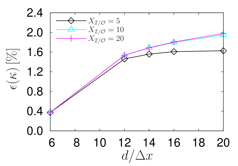
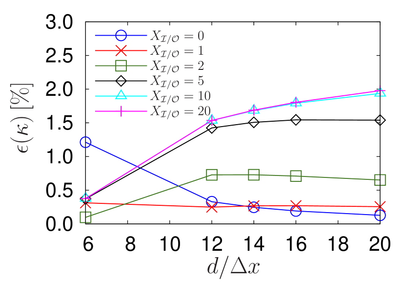
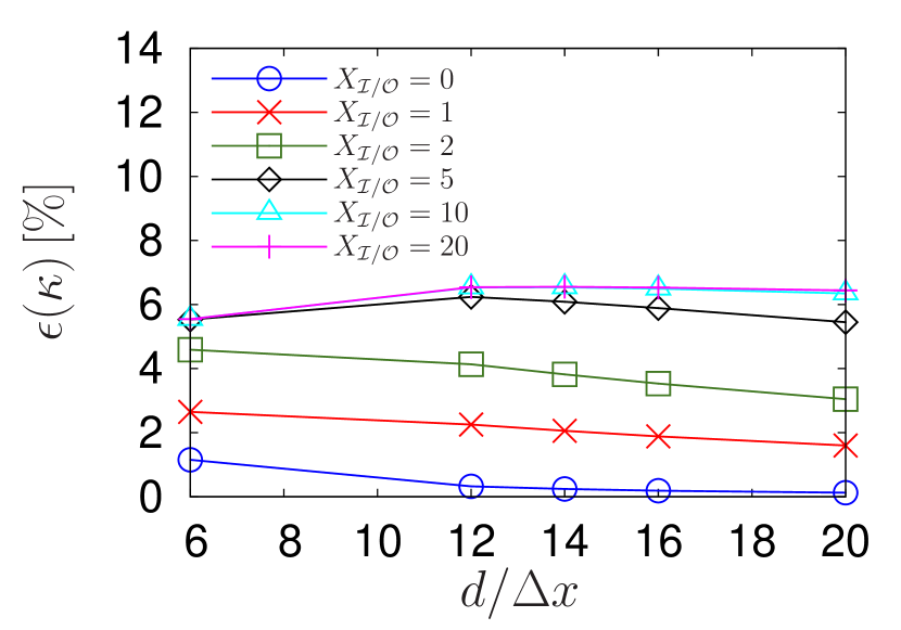
Fig. 4 shows the relative error of the computed permeabilities for chambers of different length and the three different setups presented. In case of $p$-BC and I-Ch the results are very accurate and the error stays below 2.5%. For $\nabla p$-S, however, there is a strong dependency of the results on the length of the chamber. If the sample is not periodic as it would be for experimentally relevant samples such as a discretization of a sandstone, it is not possible to avoid the chambers completely. In fact, the chambers are then absolutely needed providing a fluid reservoir before and after the sample, but as can be seen in Fig. 4 $\nabla p$-S, they produce a massive loss in accuracy. For this reason we do not take into account the $\nabla p$-S setup for further calculations. Our finding is of particular interest because this setup is the most popular one in the literature on permeability measurements using the LB method.

On the other hand, for the results obtained by alternatives $p$-BC and I-Ch, one should take into account that the major error in permeability estimation of a real sample with the LB method is due to the discretization of the porous space. For the 3D Poiseuille flow in a square pipe this error is minimal since the pipe is aligned with the lattice. Therefore, a systematic error of the order of 2% is satisfactory.

To estimate the effect of the chamber length on the permeability results when the $\nabla p$-S setup is being used, we simulate a 2D Poiseuille flow to compare the velocity field $\mathrm{u}_{x_{1}}$ obtained inside the sample when chambers of two different lengths are used. To visualize the difference a relative error field $\boldsymbol{\epsilon}$ is calculated as

$$\boldsymbol{\epsilon}(\mathbf{x},A,B)=\frac{|\mathrm{u}_{x_{1}}(\mathbf{x},X_{\mathcal{I}/\mathcal{O}}=A)-\mathrm{u}_{x_{1}}(\mathbf{x},X_{\mathcal{I}/\mathcal{O}}=B)|}{\mathrm{u}_{x_{1}}(\mathbf{x},X_{\mathcal{I}/\mathcal{O}}=A)},$$ (30)

where $A$ and $B$ represents the two chamber lengths whose velocity field $\mathrm{u}_{x_{1}}$ are being compared. Fig. 5 displays two examples comparing the results of $X_{\mathcal{I}/\mathcal{O}}=0$ and $X_{\mathcal{I}/\mathcal{O}}=2$, and the results of $X_{\mathcal{I}/\mathcal{O}}=2$ and $X_{\mathcal{I}/\mathcal{O}}=10$. As can be clearly seen, the difference of permeability estimation when using different chamber lengths, can be explained by the influence of the chamber geometry on the velocity fields $\mathrm{u}_{x_{1}}$. Not only the velocity field entering the sample is dependent on the chamber length, but also the velocity field inside the sample, where the parabolic profile is already adopted. This issue is clearly shown in both examples of Fig. 5, where a constant relative difference in the velocity field $\mathrm{u}_{x_{1}}$ remains up to the fifth node inside of the sample. It is actually this difference, which responds to how the fluid enters the sample, that is responsible for the dependency of the permeability on the length of the chamber. This clearly explains the results shown in Fig. 4 $\nabla p$-S.

$\boldsymbol{\epsilon}(\mathbf{x},0,2)$

$\boldsymbol{\epsilon}(\mathbf{x},2,10)$

Figure 5: Two examples comparing the difference in the velocity field $\mathrm{u}_{x_{1}}$ obtained in a 2D Poiseuille flow $d/\Delta x=10$ when the fluid is driven using $\nabla p$-S and two different chamber lengths $X_{\mathcal{I}/\mathcal{O}}$ are used. The difference is calculated using the relative error field $\boldsymbol{\epsilon}(\mathbf{x},A,B)$ presented in Eq. (30). For both examples, the velocity field $\mathrm{u}_{x_{1}}$ is only comparable in the zone that both domains have in common and which is defined by the shortest chamber. On the $x_{AJ}$-axis the first and last nodes inside the sample $\mathcal{S}$ represent the solid walls defining the pipe. Although the major difference resides at the inlet, a constant relative error remains inside the sample, which is responsible for the difference in the measured permeability.

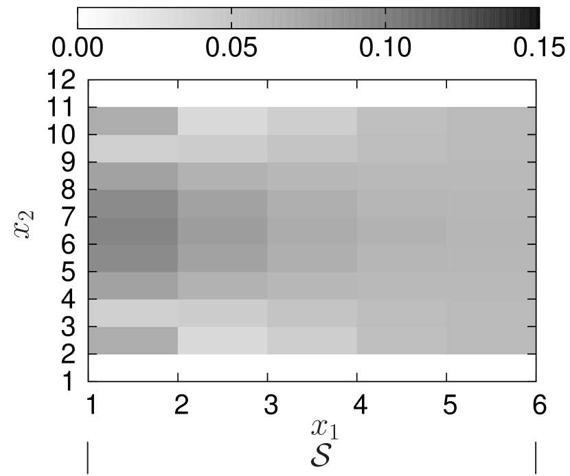
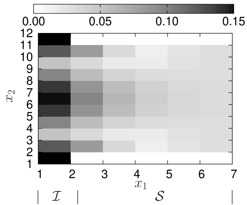
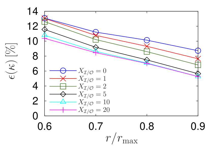
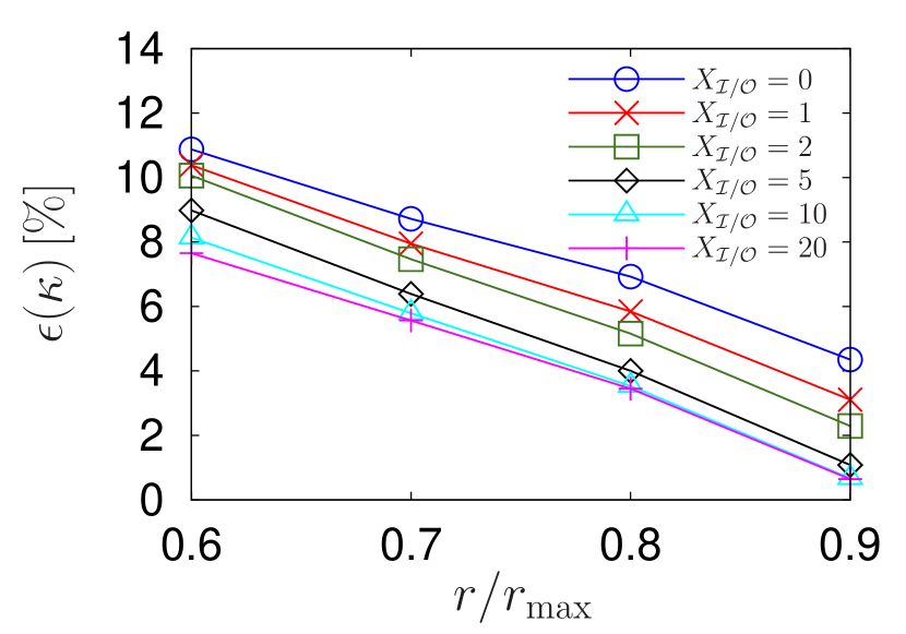
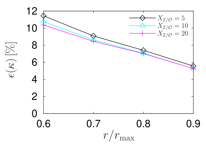
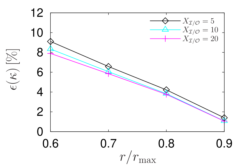
Fig. 6 displays the permeability calculated for a BCC cubic array using the LB-BGK and LB-MRT method and the alternatives $p$-BC and I-Ch with different chamber length. In contrast to the 3D Poiseuille flow, the measurements suffer indeed from an error due the domain discretization. As in Fig. 4 for the 3D Poiseuille flow, the dependency of the results using I-Ch on the length of the chambers is narrower than using $p$-BC for both LB methods.

As it was stressed above, typically the major contribution to the error of permeabilities estimated using the LB method is the discretization. This issue is clearly seen in Fig. 6 where the relative error in the permeability estimation increases if the radius of the sphere is decreased, which is equivalent to reducing the resolution.

The LB-MRT method in general produces more accurate results than LB-BGK. The best results can be obtained when using LB-MRT together with I-Ch and $X_{\mathcal{I}/\mathcal{O}}=20$. However, reducing the channel length does not have a strong influence. On the other hand, if we compare the results yield by using I-Ch with the ones obtained with $p$-BC, only minor differences can be obtained for identical chamber lengths. Following this we can assert that there is no significant difference in accuracy when using either I-Ch or $p$-BC, as it was also expected from the data presented in Fig. 4. The parameter impacting on the accuracy is the chamber length. The LB-MRT together with $p$-BC without chambers achieves the same accuracy as LB-BGK with I-Ch, but in the latter case chambers are required. Since long chambers increase the computational domain, they are a burden in terms of computational effort. Thus, it is important to understand their influence in order to decide whether a lower accuracy can be accepted if the computational effort is substantially reduced.

Pressure BC ($p$-BC)

LB-BGK

LB-MRT

Injection Channel (I-Ch)

LB-BGK

LB-MRT

Figure 6: Relative error of permeability for a BCC cubic array of spheres. The alternatives $p$-BC, I-Ch are being tested together with different lengths of the chambers $\mathcal{I}$ and $\mathcal{O}$ and also using the LB-BGK and LB-MRT method. The LB-MRT together with $p$-BC without chambers achieves the same accuracy as using LB-BGK with I-Ch, but in the latter case chambers are required.

The efficiency of the LB-implementations, i.e., pore-matrix and pore-list as their memory demands explained above are directly related to the porosity of the sample. It is important to stress that the efficiency is independent of the setup used for the permeability estimation but it depends on the LB method used, i.e., BGK or MRT. In the case of using LB-BGK instead of LB-MRT the CPU time required decreases by 15%–20% bib:cf.CPaLLuCMi.2006 .

The use of chambers and more precisely their lengths determine the porosity of the whole computational domain. For example, if in a cubic sample representing a realistic porous medium with porosity $\phi=10\%$ we add chambers with lengths 5% of the sample length, we obtain a computational domain with porosity $\phi\approx 18.2\%$. Even more dramatically is the case if the sample has a smaller porosity. If we add chambers with the same length explained above to a cubic sample with porosity $\phi=5\%$, the total porosity would increase by a factor of $\sim\!\!\!173\%$. Since the efficiency of both LB-implementations scales linearly with the porosity, the use of chambers is expensive in terms of computational cost and should be avoided if possible. For low porosity values, as realistic samples have, the pore-list implementation is more efficient than pore-matrix. On the other hand, for more open domains, as pipes for example, the pore-matrix data structure is more efficient since it does not require the connection matrix. A quantitative comparison of the computation efficiency is not easily possible. Even though it is possible to calculate for both implementations the number of floating-point operations necessary to perform a single time step, a quantitative analysis of the performance of two idependent codes is not as straightforward: the code performance strongly depends on the actual implementation details, memory access patterns and in particular also on the cache performance of the used architecture.

8 Conclusions

We presented different alternative setups to estimate the permeability of a porous medium, which utilize an injection channel (I-Ch), pressure boundary conditions ($p$-BC), or a force density applied in the sample volume ($\nabla p$-S). The setups differ on how the fluid is driven and how the pressure gradient is being estimated. Further, the accuracy of the LB-BGK and LB-MRT method together with different setups with variable chamber length, has been investigated. Another point that has been stressed is the efficiency of the LB-implementations comparing the standard implementation using a pore-matrix data structure with a pore-list code to represent the geometry.

Our findings show that the use of $\nabla p$-S as an alternative for permeability estimation should not be taken into account due to the need of chambers as fluid reservoir together with the strong dependency of the results on the length of these chambers. This is an important result since driving the fluid by using a body force applied in the sample volume is probably the most popular approach in the literature on permeability calculations using the LB method.

Further, the pore-list implementation allows to reduce the computational effort required to simulate fluid flows in porous media substantially if the porosity of the porous medium is small.

Finally, taking into account the extra computational effort added because of the number of required lattice nodes when chambers are used, it is highly recommended to completely eliminate them by using $p$-BC. A resulting compromise in the accuracy can be resolved by using the LB-MRT method. For this reason in the case of facing the permeability estimation of a realistic media, pore-list, $p$-BC, and LB-MRT is the combination suggested by the authors taking into account the computational domain size, accuracy and required computer time.

References

- (1) G. R. McNamara and G. Zanetti. Use of the Boltzmann equation to simulate lattice-gas automata. Phys. Rev. Lett., 61(20):2332–2335, 1988.
- (2) F. J. Higuera, S. Succi, and R. Benzi. Lattice gas dynamics with enhanced collisions. Europhys. Lett., 9(4):345–349, 1989.
- (3) H. Chen, S. Chen, and W. H. Matthaeus. Recovery of the Navier-Stokes equations using a Lattice-gas Boltzmann method. Phys. Rev. A, 45(8):R5339–R5342, 1992.
- (4) Y. H. Qian, D. d’Humières, and P. Lallemand. Lattice BGK models for Navier-Stokes equation. Europhys. Lett., 17(6):479–484, 1992.
- (5) S. Chen, H. Chen, D. Martínez, and W. H. Matthaeus. Lattice Boltzmann model for simulation of magnetohydrodynamics. Phys. Rev. Lett., 67(27):3776–3779, 1991.
- (6) S. Succi. The lattice Boltzmann equation for fluid dynamics and beyond. Oxford University Press, 2001.
- (7) S. Succi, E. Foti, and F. Higuera. Three-dimensional flows in complex geometries with the lattice Boltzmann method. Europhys. Lett., 10(5):433–438, 1989.
- (8) N. S. Martys and E. J. Garboczi. Length scales relating the fluid permeability and electrical conductivity in random two-dimensional model porous media. Phys. Rev. B, 46(10):6080–6090, 1992.
- (9) O. van Genabeek and D. H. Rothman. Macroscopic manifestations of microscopic flows through porous media: phenomenology from simulation. Annu. Rev. Earth and Planetary Sci., 24:63–87, 1996.
- (10) A. Koponen, M. Kataja, and J. Timonen. Permeability and effective porosity of porous media. Phys. Rev. E, 56(3):3319–3325, 1997.
- (11) B. Ferréol and D. H. Rothman. Lattice-Boltzmann simulations of flow through Fontainebleau sandstone. Transp. Porous Media, 20(1-2):3–20, 1995.
- (12) N. S. Martys, J. G. Hagedorn, D. Goujon, and J. E. Devaney. Large scale simulations of single and multi-component flow in porous media. In Developments in X-Ray Tomography II, Proceeding of SPIE, volume 3772, pages 205–213, 1999.
- (13) C. Manwart, U. Aaltosalmi, A. Koponen, R. Hilfer, and J. Timonen. Lattice-Boltzmann and finite-difference simulations for the permeability of three-dimensional porous media. Phys. Rev. E, 66(1):016702, 2002.
- (14) J. Harting, M. Venturoli, and P. Coveney. Large-scale grid-enabled lattice-Boltzmann simulations of complex fluid flow in porous media and under shear. Phil. Trans. R. Soc. Lond. A, 362:1703–1722, 2004.
- (15) B. Ahrenholz, J. Tölke, and M. Krafczyk. Lattice Boltzmann simulations in reconstructed parametrized porous media. Int. J. Comp. Fluid Dyn., 20(6):369–377, 2006.
- (16) A. Koponen, D. Kandhai, E. Hellén, M. Alava, A. Hoekstra, M. Kataja, K. Niskanen, P. Sloot, and J. Timonen. Permeability of three-dimensional random fiber webs. Phys. Rev. Lett., 80(4):716–719, 1998.
- (17) H. Darcy. Les fontaines publiques de la ville de Dijon. Dalmont, Paris, 1856.
- (18) S. Donath, T. Zeiser, G. Hager, J. Habich, and G. Wellein. Optimizing performance of the lattice Boltzmann method for complex structures on cache-based architectures. In Frontiers in Simulation: Simulationstechnique - 18th Symposium in Erlangen, pages 728–735, 2005.
- (19) P. L. Bhatnagar, E. P. Gross, and M. Krook. Model for collision processes in gases. I. small amplitude processes in charged and neutral one-component systems. Phys. Rev., 94(3):511–525, 1954.
- (20) D. d’Humières, I. Ginzburg, M. Krafczyk, P. Lallemand, and L.-S. Luo. Multiple-relaxation-time lattice Boltzmann models in three dimensions. Phil. Trans. R. Soc. Lond. A, 360(1792):437–451, 2002.
- (21) D. Hänel. Molekulare Gasdynamik: Einführung in die kinetische Theorie der Gase und Lattice-Boltzmann-methoden. Springer, 2004.
- (22) P. Lallemand and L.-S. Luo. Theory of the lattice Boltzmann method: dispersion, dissipation, isotropy, Galilean invariance, and stability. Phys. Rev. E, 61(6):6546–6562, 2000.
- (23) Z. Guo, C. Zheng, and B. Shi. Discrete lattice effects on the forcing term in the lattice Boltzmann method. Phys. Rev. E, 65(4):046308, 2002.
- (24) Q. Zou and X. He. On pressure and velocity boundary conditions for the lattice Boltzmann BGK model. Phys. Fluids, 9(6):1591–1598, 1997.
- (25) M. Hecht and J. Harting. Implementation of on-site velocity boundary conditions for D3Q19 lattice Boltzmann simulations. J. Stat. Mech.: Theor. Exp., 2010(01):P01018, 2010.
- (26) M. E. Kutay, A. H. Aydilek, and E. Masad. Laboratory validation of lattice Boltzmann method for modeling pore-scale flow in granular materials. Comp. and Geotechnics, 33(8):381–395, 2006.
- (27) T. W. Patzek and D. B. Silin. Shape factor and hydraulic conductance in noncircular capillaries. i. one-phase creeping flow. J. Colloid Int. Sci., 236(2):295–304, 2001.
- (28) H. Hasimoto. On the periodic fundamental solutions of the stokes equations and their application to viscous flow past a cubic array of spheres. J. Fluid Mech., 5(2):317–328, 1959.
- (29) A. S. Sangani and A. Acrivos. Slow flow through a periodic array of spheres. Int. J. of Muliphase Flow, 8(4):343–360, 1982.
- (30) C. Pan, L.-S. Luo, and C. T. Miller. An evaluation of lattice Boltzmann schemes for porous medium flow simulation. Computers & Fluids, 35:898–909, 2006.
- (31) I. Ginzburg and D. d’Humières. Local second-order boundary methods for lattice Boltzmann models. J. Stat. Phys., 84(5-6):927–971, 1996.
- (32) A. Narváez, T. Zauner, F. Raischel, J. Harting, and R. Hilfer. Quantitative analysis of numerical estimates for the permeability of porous media from lattice-boltzmann simulations. arXiv:1005.2530, 2010.