OU-HET 667/2010

Phenomenological Aspects of
Dirichlet Higgs Model from Extra-Dimension

Naoyuki Haba^a,, Kin-ya Oda^a,, and Ryo Takahashi^b,

^aDepartment of Physics, Graduate School of Science, Osaka University,
Toyonaka, Osaka 560-0043, Japan
^bMax-Planck-Institut f$\ddot{u}$r Kernphysik, Postfach 10 39 80, 69029
Heidelberg, Germany

Abstract
We study a simple five-dimensional extension of the Standard Model, compactified on a flat line segment in which there propagate Higgs and gauge bosons of the Standard Model. We impose a Dirichlet boundary condition on the Higgs field to realize its vacuum expectation value. Since a flat Nambu-Goldstone zero-mode of the bulk Higgs is eliminated by the Dirichlet boundary condition, a superposition of the Higgs Kaluza-Klein modes play the role of the Nambu-Goldstone boson except at the boundaries. We discuss phenomenology of our model at the LHC, namely the top Yukawa deviation and the production and decay of the physical Higgs field, as well as the constraints from the electroweak precision measurements.

1 Introduction

Extra-dimensional theory is an interesting candidate beyond the Standard Model (SM), having rich phenomenology of Kaluza-Klein (KK) particles, a tower of modes for each SM field propagating in bulk. Especially, in the Universal Extra Dimensions (UED) model [1], the lightest KK particles (LKP) with an odd parity is stable and can be a candidate for the dark matter. The UED can also lower constraints on the compactification scale from the electroweak (EW) precision measurements to few hundred GeV due to the five-dimensional (5D) Lorentz symmetry [2, 3], while the scale is restricted to be larger than few TeV for the brane localized fermion (BLF) scenario [4]-[9]. If the KK-modes are confirmed at the CERN LHC experiment, it would strongly indicate the existence of the extra dimensions.

On the other hand, anther interesting phenomenological consequence of the extra-dimensional theory is the top Yukawa deviation, which is a deviation of the Yukawa coupling between top quark and physical Higgs field from the naive SM expectation: $m_{t}/v_{\text{EW}}$. Such a deviation is generally caused when there are several Higgs doublets. Recently it has been pointed out that the deviation can be induced from effects of the brane localized Higgs potentials [10, 11] and the Dirichlet boundary condition (BC) [12] in a simple setup of the extra-dimensional theory with one Higgs doublet.

In this paper, we study a 5D model [12] where the gauge bosons and Higgs doublet of the SM exist in the 5D bulk compactified on a line segment with a flat metric, imposing a generic Dirichlet BC for the Higgs and Neumann BC for all other SM fields. The vacuum expectation value (VEV) of the Higgs is induced from the Dirichlet BC which is generally allowed in higher dimensional theories. We present wave-function profiles of bulk fields under these BCs. The Dirichlet BC removes the Higgs zero-mode and one might worry how a Nambu-Goldstone (NG) boson is supplied for the electroweak symmetry breaking. We show that a superposition of sufficiently large number of KK-modes gives a correct wave-function profile which is flat except at the boundaries.

We consider the case where all other SM fermions propagate in the bulk as the UED model. Then, we will give detailed phenomenology of the model on the top Yukawa deviation, the production and decay of Higgs, constraints on the model from the electroweak precision measurements, and dark matter.

The organization of the paper is as follows. In the next section, we present our extra-dimensional setup and show the profiles, masses and couplings of bulk Higgs and gauge fields. In Section 3, we discuss phenomenological aspects of the setup such as top Yukawa deviation, the production and decay of the Higgs, constraints from the EW precision measurements, and dark matter candidate. In Section 4, we summarize our results. In Appendix we show the 5D gauge and Higgs kinetic Lagrangian and the gauge fixing.

2 Bulk Higgs and its profiles

Our setup is that the SM Higgs doublet exists in the 5D flat space-time with Dirichlet BC. We study the Higgs wave-function profiles, masses and couplings at first. Our analysis is applicable in more general cases though we will focus on the case where EW symmetry is broken through the extra-dimensional BC.

2.1 VEV profile

Let us show wave-function profile of classical mode, i.e. the VEV, of a bulk scalar field. Start from an illustrative example of the bulk complex scalar $\Phi$ with the kinetic action

$$S=-\int d^{4}x\int_{-L/2}^{+L/2}dz\,\left|\partial_{M}\Phi\right|^{2},$$ (1)

where we write 5D coordinates as $x^{M}=(x^{\mu},z)$ with $M,N,\ldots$ running from 0 to 4 and $\mu,\nu,\ldots$ running from 0 to 3. The 5D spacetime is compactified on a line segment and the action is defined in $-L/2\leq z\leq+L/2$.

Now let us impose a Dirichlet BC for the bulk scalar field. We consider the action, along with all the BCs, is invariant under the KK parity, $z\to-z$. A compactification on the line segment with the Dirichlet BC [12] derives different physics from the orbifold $S^{1}/Z_{2}$ compactification with a brane-localized potential in an infinitely large coupling limit [10], since the former does not have the uncontrollably large interactions involving the NG-boson as we will see.

Rewriting in terms of real fields, $\Phi=(\Phi_{R}+i\Phi_{I})/\sqrt{2}$, the variation of the action reads

$$\delta S=\int d^{4}x\int_{-L/2}^{+L/2}dz\bigg{[}\delta\Phi_{X}(\mathcal{P}\Phi_{X})+\delta(z-\frac{L}{2})\delta\Phi_{X}(-\partial_{z}\Phi_{X})+\delta(z+\frac{L}{2})\delta\Phi_{X}(+\partial_{z}\Phi_{X})\bigg{]},$$ (2)

where $\mathcal{P}\equiv\Box+\partial_{z}^{2}$. The VEV of the scalar field $\Phi^{c}$ is determined by the action principle $\delta S=0$, that is, $\mathcal{P}\Phi_{X}^{c}=0$. The general solution of this Equation of Motion (EoM) is $\Phi^{c}(z)=A+Bz$. The undetermined coefficients $A$ and $B$ can be fixed by choosing BCs at $z=\pm L/2$. We have four choices of combination of Dirichlet and Neumann BCs at $z=\pm L/2$, namely,

$$(D,D),~{}~{}~{}(D,N),~{}~{}~{}(N,D),~{}~{}~{}\mbox{and}~{}~{}~{}(N,N),$$ (3)

where $D$ and $N$ denote the Dirichlet and Neumann BCs, respectively. These BCs are written as

$$\delta\Phi|_{z=\xi}=0,$$ (4)

for the Dirichlet BC, and

$$\partial_{z}\Phi|_{z=\xi}=0,$$ (5)

for the Neumann BC, where $\xi$ is taken as $+L/2$ or $-L/2$ in each case. Difference choice of BC corresponds to different choice of theory. A theory is fixed once one chooses one of the four patterns of BC conditions.

In this paper, we will take the following $(D,D)$ BC for a scalar field,

$$\delta\Phi|_{z=\pm L/2}=0\;\;\;{\rm and}\;\;\;\Phi|_{z=\pm L/2}=v$$ (6)

on both branes, where $v$ is a free complex constant of mass dimension $[3/2]$. Notice that these BCs are the most general form of Dirichlet BCs which are consistent with the action principle. Here, we can determine the solution of EoM under these BCs as

$$\Phi^{c}(z)=v,$$ (7)

so that the VEV profile on the extra-dimensional direction is flat. How about the profiles of quantum modes of the physical Higgs and NG bosons?

2.2 Profiles of physical Higgs and others

Let us investigate wave-function profiles of its quantum fluctuation modes that correspond to the physical Higgs and NG modes by regarding $\Phi$ as the bulk SM Higgs doublet. The most general form of the Dirichlet BC on $\Phi(x,z)$ is

$$\delta\Phi(x,\pm{L\over 2}) =0, \Phi(x,\pm{L\over 2}) =\left(\begin{array}[]{c}v_{1}\\ v_{2}\end{array}\right),$$ (10)

where $v_{1}$ and $v_{2}$ are free complex constants. Without loss of generality, we can always take a basis by an $SU(2)_{L}\times U(1)_{Y}$ field redefinition so that the BCs become

$$\delta\Phi(x,\pm{L\over 2}) =0,$$ (11)

$$\Phi(x,\pm{L\over 2}) =\left(\begin{array}[]{c}0\\ v\end{array}\right),$$ (14)

and thus, the resultant VEV profile is given by

$$\Phi^{c}(z)=\left(\begin{array}[]{c}0\\ v\end{array}\right).$$ (17)

The Higgs doublet $\Phi$ is KK-expanded around the VEV in Eq.(17) by infinite number of 4D fields as

$$\Phi(x,z)=\left(\begin{array}[]{c}\displaystyle\sum_{n=0}^{\infty}f_{n}^{\varphi^{+}}(z)\varphi_{n}^{+}(x)\\ v+\frac{1}{\sqrt{2}}\displaystyle\sum_{n=0}^{\infty}[f_{n}^{H}(z)H_{n}(x)+if_{n}^{\chi}(z)\chi_{n}(x)]\end{array}\right),$$ (20)

where we took $\Phi_{R}/\sqrt{2}=v$ and $\Phi_{I}=0$ in the language of the previous subsection, and $H_{n}(x)$ are the physical Higgs scalar. A linear combination of $\chi_{n}(x)$ and $Z_{z}^{(n)}(x)$ and that of $\varphi_{n}^{+}(x)$ and $W_{z}^{(n)+}(x)$ are, respectively, absorbed as the longitudinal component of $Z_{\mu}^{(n)}$ and $W_{\mu}^{(n)+}$, where $Z_{z}$ and $W_{z}$ are the fifth components of 5D $Z$ and $W$ bosons. Notice that the orthogonal combinations to above ones are the physical neutral pseudo-scalar and charged bosons, respectively.

The 5D action for $H(x,z)$ can be written as

$$S_{H} = \int d^{4}x\int_{-L/2}^{+L/2}dz\bigg{[}\frac{1}{2}H(\Box+\partial_{z}^{2})H+\frac{\delta(z-L/2)}{2}H(-\partial_{z}H)$$ (21)

$$\phantom{\int d^{4}x\int_{-L/2}^{+L/2}dz\bigg{[}\frac{1}{2}H(\Box+\partial_{z}^{2})H}+\frac{\delta(z+L/2)}{2}H(+\partial_{z}H)\bigg{]},$$

and the KK equation for the physical Higgs is given by

$$\partial_{z}^{2}f_{n}^{H}(z)=-\mu_{Hn}^{2}f_{n}^{H}(z),$$ (22)

where general solution of this KK equation is

$$f_{n}^{H}(z)=\alpha_{n}\cos(\mu_{Hn}z)+\beta_{n}\sin(\mu_{Hn}z).$$ (23)

Taking the Dirichlet BCs in Eq.(11) for quantum fluctuation, we obtain

$$f_{n}^{H}(z=\pm L/2)=0,$$ (24)

and hence the wave-function profiles become

$$f_{n}^{H}(z)=\left\{\begin{array}[]{ll}\sqrt{\frac{2}{L}}\cos\left(\frac{(n+1)\pi}{L}z\right)&\mbox{ for even }n,\\ \sqrt{\frac{2}{L}}\sin\left(\frac{(n+1)\pi}{L}z\right)&\mbox{ for odd }n.\end{array}\right.$$ (27)

They are are shown in Table 1. It is worth noting that the wave-function profile of the lowest ($n=0$) mode, which corresponds to the SM-like Higgs, is described by a cosine function,

$$f_{0}^{H}(z)=\sqrt{\frac{2}{L}}\cos\left(\frac{\pi}{L}z\right).$$ (28)

Notice that, if we took Neumann BC for the Higgs, the flat profile of the lowest mode appears.

Typical profiles of Higgs field
$n=0$	$n=1$	$n=2$	$n=3$

Table 1: The wave-function profiles of the physical Higgs

This is one of the interesting results from this simple setup of taking Dirichlet BC for the bulk Higgs doublet, and this property leads to interesting phenomenology such as the top Yukawa deviation.

The $n$-mode Higgs mass is calculated as

$$m_{H^{(n)}}^{2}=-\int_{-L/2}^{+L/2}dzf_{n}^{H}(z)\partial_{z}^{2}f_{n}^{H}(z)=\left(\frac{(n+1)\pi}{L}\right)^{2},$$ (29)

where the mass of the lowest ($n=0$) mode Higgs becomes the KK scale:

$$m_{KK}\equiv\frac{\pi}{L}.$$ (30)

This feature of KK-scale Higgs mass is the specific result induced from the Dirichlet BC in Eq.(24). Note that one does not have a theoretical constraint on the magnitude of the Higgs mass from the discussions of perturbative unitarity as in the SM since the mass depends on the compactification scale but not on the Higgs self-coupling (see, footnote 2).

Profiles of $n$-mode of $\chi^{(n)}$ and $\varphi^{+}{}^{(n)}$ are the same as $H^{(n)}$, because the 5D action of $\chi(x)$ and $\varphi^{+}(x)$ have the same form as that of $H(x)$. Therefore, $f_{n}^{\chi}(z)$ and $f_{n}^{\varphi^{+}}(z)$ also obey the same KK equations as $f_{n}^{H}(z)$. Taking this Dirichlet BC is similar to introducing an extra fake Higgs field $\phi$ which is localized at the boundary and couples to the bulk Higgs doublet as $|\phi|^{2}\left(|\Phi|^{2}-v^{2}\right)$ and with a limit of $|\langle\phi\rangle|\rightarrow\infty$. But, a crucially different point is that the three- and four-point Higgs self-couplings of $HHH$, $H\chi\chi$, $H\varphi^{+}\varphi^{-}$, $HHHH$, $HH\chi\chi$, $HH\varphi^{+}\varphi^{-}$, $\chi\chi\chi\chi$, $\chi\chi\varphi^{+}\varphi^{-}$, and $\varphi^{+}\varphi^{-}\varphi^{+}\varphi^{-}$ vanish in the current model, since there is no Higgs potential. (Here and hereafter we represent the lowest KK-modes of the bulk Higgs by $H(x)$, $\chi(x)$, and $\varphi^{+}(x)$, for simplicity.) It means that longitudinal components of gauge bosons, $W_{L}$ and $Z_{L}$, interact only through the gauge couplings.

2.3 Profiles of gauge fields

Next, we show the gauge sector. We take usual Neumann BC for the gauge fields as

$$\partial_{z}A_{\mu}(z)|_{z=\pm L/2}=0\;\;\;{\rm and}\;\;\;A_{z}(z)|_{z=\pm L/2}=0.$$ (31)

The gauge boson masses are derived from the Higgs kinetic term as

$$S_{\mbox{{\scriptsize kin}}}=\int d^{4}x\int_{-L/2}^{+L/2}dx|D_{M}\Phi|^{2}$$ (32)

with the covariant derivative

$$D_{M}\equiv\partial_{M}+ig_{5}W_{M}^{a}T^{a}+ig_{5}^{\prime}B_{M}Y,$$ (33)

where the 5D gauge couplings are related to the 4D ones by $g_{5}=g\sqrt{L}$ and $g_{5}^{\prime}=g^{\prime}\sqrt{L}$. The SM gauge bosons are given by

$$Z_{M}\equiv\frac{g_{5}W_{M}^{3}-g_{5}^{\prime}B_{M}}{\sqrt{g_{5}+g_{5}^{\prime}}},~{}~{}~{}A_{M}\equiv\frac{g_{5}W_{M}^{3}+g_{5}^{\prime}B_{M}}{\sqrt{g_{5}+g_{5}^{\prime}}},~{}~{}~{}W_{M}^{\pm}\equiv\frac{W_{M}^{1}\mp iW_{M}^{2}}{\sqrt{2}}.$$ (34)

Therefore, the KK equation for the weak bosons become

$$\left[\partial_{z}-\frac{v^{2}}{2}(g_{5}^{2}+g_{5}^{\prime}{}^{2})\right]f_{n}^{Z}(z) = -\mu_{Zn}^{2}f_{n}^{Z}(z),$$ (35)

$$\left[\partial_{z}-\frac{v^{2}}{2}g_{5}^{2}\right]f_{n}^{W}(z) = -\mu_{Wn}^{2}f_{n}^{W}(z).$$ (36)

It is seen that the Neumann BCs for the gauge fields guarantees the flatness of profiles of the zero-mode gauge fields. Then, the usual gauge boson masses are given by

$$m_{Z}^{2}=\frac{(g^{2}+g^{\prime}{}^{2})v_{\mbox{{\scriptsize EW}}}^{2}}{2},~{}~{}~{}m_{W}^{2}=\frac{g^{2}v_{\mbox{{\scriptsize EW}}}^{2}}{2},$$ (37)

where $v=v_{\mbox{\scriptsize EW}}/\sqrt{L}$. The masses of $n$th KK-modes are described as

$$m_{Z^{(n)}}=m_{Z}^{2}+n^{2}m_{KK}^{2},~{}~{}~{}~{}~{}m_{W^{(n)}}=m_{W}^{2}+n^{2}m_{KK}^{2},$$ (38)

and we find that the $n$-mode Higgs mass is the same as the $(n+1)$-mode KK gauge boson masses. The frequency of $n$-mode Higgs profile is also the same as that of $(n+1)$-mode KK gauge bosons’ profiles (see footnote 2). These results are originating from the Dirichlet (Neumann) BC for the bulk Higgs (gauge) field.

Here we focus on the Higgs mechanism of the zero-mode gauge bosons in more detail. As discussed above, although the VEV itself has a flat profile, the 5D fields $\chi(x,z)$ and $\varphi^{\pm}(x,z)$ have not zero-mode. Notice also that the lowest mode of the $W_{\mu}^{\pm}(x,z)$ and $Z_{\mu}(x,z)$ are flat at the tree level. Therefore, $\varphi$ and $\chi$ must somehow yield the flat profile to be absorbed into $W_{\mu}^{(0)\pm}$ and $Z_{\mu}^{(0)}$. Key observation is that the NG-boson that is absorbed by the zero-mode $W$ (or $Z$) is composed by a linear combination of $n=0$ to $\infty$ modes of NG boson. For example, $Z_{L}^{(0)}$ absorbs the following field having flat profile along the 5D direction except at the boundary,

$$\chi(x,z)=0,\hskip 42.67912pt(z=\pm L/2),$$ (39)

$$\chi(x,z)=\chi_{\text{NG}}(x),~{}~{}~{}(-L/2<z<L/2),$$ (40)

which can be realized by a superposition of the infinite number of modes

$$\chi(x,z)=\sum_{n=0}^{\infty}f_{n}^{\chi}(z)\chi_{n}(x),$$ (41)

where

$$\chi_{n}(x)=\frac{2\sqrt{2L}(-1)^{n/2}}{(n+1)\pi}\chi_{\text{NG}}(x),$$ (42)

for even $n$. By rewriting $n=2m$, we can show

$$\chi(x,z)=\chi_{\text{NG}}(x)\sum_{m=0}^{\infty}\frac{4(-1)^{m}}{(2m+1)\pi}\cos\left(\frac{(2m+1)\pi}{L}z\right).$$ (43)

This profile exactly realizes the flat profile in Eqs.(39) and (40).

The 5D gauge theory is non-renormalizable and hence is defined with a ultraviolet cutoff. Therefore, one might think that the sum should be taken up to a finite value of $m$ corresponding to a cutoff scale $\Lambda=mm_{KK}=m\pi/L$. Let us see the correspondence between the cutoff scale $\Lambda$, equivalently the maximum $m$, and the flatness of the would-be NG mode $\chi(x,z)$, which is represented in Fig. 1.

(a)                                                                (b)

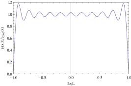
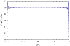
(c)                                                                (d)

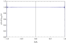
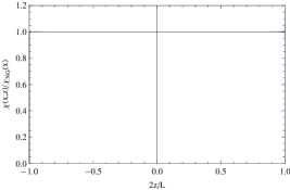
Figure 1: The relation between the flatness of VEV profile and largeness of $m$. The horizontal and vertical axes are $2z/L$ and $\chi(x,z)/\chi_{\text{NG}}(x)$, respectively, in all figures. The figure (a) corresponds to the case of $m=10$, (b) for $m=100$, (c) for $m=1000$, and (d) for $m=10000$.

In our setup, the KK scale is a model parameter constrained from the precision EW measurements. For example, when $m=10^{4}$ and $m_{KK}=600$ ($4\times 10^{3}$) GeV are taken, the cutoff scale of this setup becomes $\Lambda=6\times 10^{3}$ ($4\times 10^{4}$) TeV.

Then, what should we think the 5D cutoff? There must exist heavier KK-modes than the cutoff scale in principle, otherwise the complete flat profile of NG bosons could not be obtained. There is generally a high energy cutoff in this 5D model so that we cannot sum over infinite number of KK-modes. However, a model with a cutoff $\Lambda$ is expected to have an ambiguity of ${\mathcal{O}}(\Lambda^{-1})$, which are induced from integrating out heavier KK-modes above $\Lambda$. In order to distinguish this ambiguity, for example, deviation from flat profile in above case, we need an experimental resolution of ${\mathcal{O}}(\Lambda^{-1})$, so that the ambiguity could be neglected.

As for longitudinal components of $W_{L}^{(n)}$ and $Z_{L}^{(n)}$ ($n\geq 1$), they are mainly composed by $W_{y}^{(n)}$ and $Z_{y}^{(n)}$, respectively. The orthogonal linear combinations are physical charged KK scalar and neutral pseudo-scalar particles, respectively.

In our model, the gauge symmetry is violated by the extra-dimensional BC of Higgs. However, the 5D gauge symmetry will be restored as an energy scale becomes much higher than the KK scale. We note that in several models of orbifold/boundary symmetry breaking, it has been shown that the longitudinal gauge boson scattering etc. are indeed unitarized by taking into account KK-mode contributions [15]-[22]. Therefore, it would be expected that the bulk gauge boson scattering is unitarized in such a region of our model (above the KK scale but lower than the 5D cut-off scale) by taking account all the relevant KK-modes.

At the end of this section, we comment on the KK parity. It is known that the UED model conserves KK parity. How about our setup? In our model, the Dirichlet BC is taken for the Higgs field, and when we take the same BC on both $z=\pm L/2$ branes, there exists a reflection symmetry between the branes. This guarantees the conservation of the KK parity in the gauge and Higgs sector. Thus, the existence of KK parity in the Lagrangian depends on a fermion sector. When the fermions are localized on the 4D branes, the KK parity is broken in general. On the other hand, the KK parity is conserved in a bulk fermion setup similar to the UED model. When KK parity exists in the model, the lightest KK parity odd particle is stable, which can be a candidate of the dark matter. We will return to this point later.

3 Phenomenological aspects

In this section, we discuss phenomenological aspects of above extra-dimensional setup, namely top Yukawa deviation, the production and decay of the Higgs, constraints from the EW precision measurements, and dark matter candidate.

3.1 Top Yukawa deviation

Let us investigate the top Yukawa deviation, which is one of the most interesting phenomenologies in our setup. First we give a brief explanation about the top Yukawa deviation. In the SM, the fermion mass terms and couplings with physical Higgs are given by

$$-\mathcal{L}_{Y}^{\mbox{{\scriptsize SM}}}\supset m_{f}\bar{f}(x)f(x)+y_{f}\frac{H(x)}{\sqrt{2}}\bar{f}(x)f(x),$$ (44)

where $m_{f}$ is the mass of a SM fermion $f(x)$. The mass of fermion is described by the VEV of the Higgs multiplied by the Yukawa coupling, $m_{f}\equiv y_{f}v_{\text{EW}}$. This Yukawa coupling also determines the magnitude of the coupling between fermion and the physical Higgs field, $y_{\bar{f}fH}\frac{H(x)}{\sqrt{2}}\bar{f}f$, and, thus

$$y_{\bar{f}fH}=y_{f}.$$ (45)

This is the simple tree level result in the SM. Among the Yukawa couplings in the SM, that of top quark is the largest. Therefore, this SM expectation in Eq.(45) should be checked by precisely observing the Higgs events related with the top quarks at the LHC. The deviation of the expectation from the SM is called top Yukawa deviation and observation of this phenomena would suggest the presence of physics beyond the SM. Here, we focus on the top quark when we discuss the Yukawa deviation.

It is well known that such a deviation can generally occur in multi-Higgs model. A popular multi-Higgs model is the Minimal Supersymmetric Standard Model (MSSM), in which the coupling of the top quark with the physical Higgs field is described as

$$-\mathcal{L}_{t}^{\mbox{{\scriptsize MSSM}}}\supset y_{t}\cos\alpha\frac{h^{0}}{\sqrt{2}}\bar{t}t,$$ (46)

while the Yukawa coupling of top quark is determined by $y_{t}=m_{t}/v_{u}$. It is seen that the additional factor, $\cos\alpha$, is multiplied to the Yukawa coupling. The physical meaning of this factor is a mixing angle between the weak eigenstate of the Higgs $(H_{u}^{0},H_{d}^{0})$ and the mass eigenstate $(h^{0},H^{0})$ where $h^{0}$ is the lightest CP-even Higgs field. Such a situation generally occurs in other multi-Higgs doublet models, but never happens in 4D one-Higgs doublet model.

In our model described with the Dirichlet BC, the Yukawa interaction for the top quark and the Higgs field are written as

$$-\mathcal{L}_{t}=y_{t,5}\int_{-L/2}^{+L/2}dz\left[v+f_{0}^{H}(z)\frac{H(x)}{\sqrt{2}}\right]\bar{t}(x,z)t(x,z).$$ (47)

The top quark mass, $m_{t}$, and effective top coupling in 4D, $y_{t}$, can be obtained as $m_{t}=y_{t,5}v$ and $y_{t}=\frac{m_{t}}{v\sqrt{L}}=\frac{y_{t,5}}{\sqrt{L}}$. Then the ratio of the top Yukawa coupling in our model to that of the SM, $r_{H\bar{t}t}$, is given by

$$r_{H\bar{t}t} = \frac{1}{\sqrt{L}}\int_{-L/2}^{L/2}dzf_{0}^{H}(z)=\frac{2\sqrt{2}}{\pi}\simeq 0.90,$$ (48)

which means the top deviation in this setup is 10% decrease from the SM. Such result can be hardly happened in other one-Higgs doublet models.

3.2 Higgs production and decay

Here we consider the SM-like Higgs production, higher KK Higgs production, and Higgs decay at the LHC experiment. At first, let us show the Higgs production processes.

3.2.1 Higgs production

The Higgs boson can be produced mainly through the following four different channels

• gluon fusion $gg\rightarrow H$ shown in Fig. 2 (a),

• vector boson fusion $qq\rightarrow qqH$ shown in Fig. 2 (b),

• associated production with the weak gauge bosons $q\bar{q}\rightarrow WH,~{}ZH$,

• associated production with the heavy quarks $gg,~{}q\bar{q}\rightarrow t\bar{t}H,~{}b\bar{b}H$ and $gb\rightarrow bH$.

(a) gluon fusion                 (b) vector boson fusion

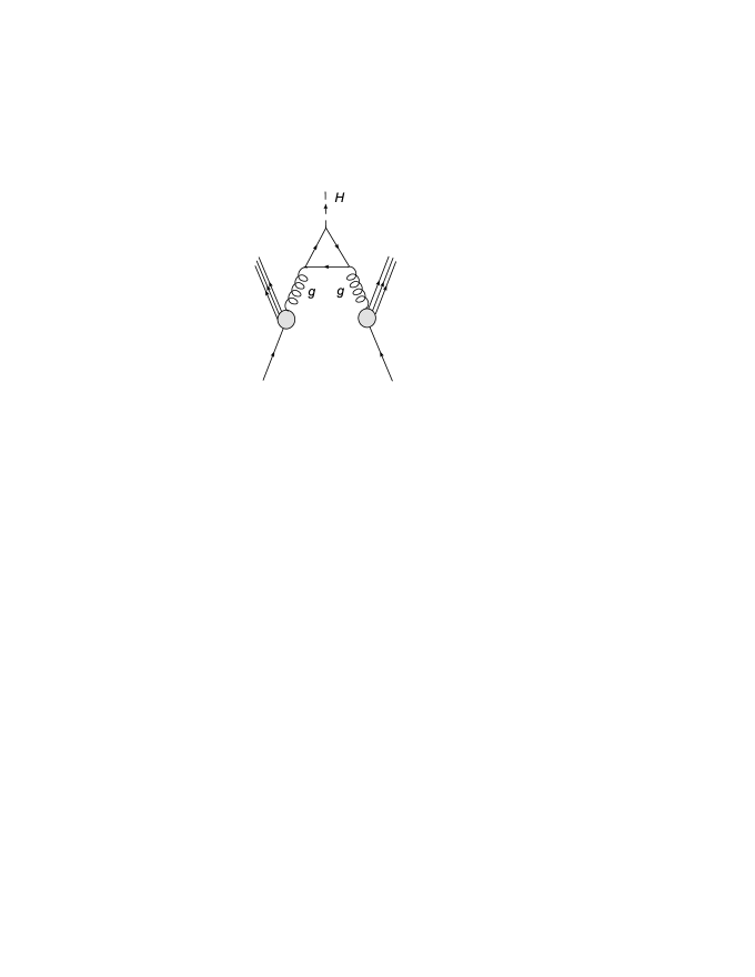
Figure 2: Dominant processes of Higgs production at the LHC

The SM predicts that the gluon fusion with the top quark 1-loop diagram dominates up to 1 TeV of Higgs mass by taking account of leading and next-to-leading order of QCD corrections with $\sqrt{s}=14$ TeV and $m_{t}=174$ GeV, while the vector boson fusion is a subdominant process for the Higgs production. So how is going in our extra-dimension scenario? Since the Yukawa couplings of Higgs with the top quark are modified, the processes for the Higgs production must be reanalyzed.

The Higgs production cross section through the gluon fusion depends on the magnitude of the coupling between the top quarks and physical Higgs boson. Since the coupling between the top quarks and Higgs boson deviates from the top Yukawa coupling as is pointed above, the cross section of the gluon fusion process becomes 81% of the SM due to $r_{H\bar{t}t}\simeq 0.81$. This is one of the most important predictions of our model. As regarding the vector boson fusion process, the magnitude of cross section changes because the coupling between $W$ and Higgs is also modified. The interaction is written by

$$-\mathcal{L}_{WWH}=\frac{em_{W}}{2\sin\theta_{W}}\frac{1}{2L}\int_{-L/2}^{+L/2}dzf_{0}^{H}(z)f_{0}^{W^{+}}f_{0}^{W^{-}}H(x)W^{+}(x)W^{-}(x)+h.c.$$ (49)

When we write the ratio of the $WWH$ coupling in the 5D model to the SM as $r_{WWH}$, it is given by

$$r_{WWH}\equiv\frac{1}{\sqrt{L}}\int_{-L/2}^{+L/2}dzf_{0}^{H}(z),$$ (50)

where we used the fact that the zero-mode profile of $W$ boson is flat $f_{0}^{W^{\pm}}(z)=1/\sqrt{L}$. Notice that this ratio is the same as $r_{H\bar{t}t}$ in Eq.(48) and its value is $\simeq 0.90$. Therefore, the cross section for the Higgs production in the model are overall decreased to $81\%$ of the SM, while the branching ratios are not changed. It is because other possible processes for the production such as $q\bar{q}\rightarrow HW$, $q\bar{q}\rightarrow HZ$, $gg,~{}q\bar{q}\rightarrow t\bar{t}H,~{}b\bar{b}H$, and $gb\rightarrow bH$ are also suppressed in the same manner.

3.2.2 Higher KK Higgs production

Let us consider the Higgs production of higher KK-modes, which might be discovered at the LHC and/or future international linear collider (ILC) experiment. In above discussions, we only consider the lightest states of Higgs and top quark propagate in the loop of the gluon fusion process. However, in general, higher KK Higgs and heavy quarks can contribute in this process.

In our model, a higher KK Higgs can be produced through the gluon fusion as

$$q^{(2n)}\bar{q}^{(2|n-l-1|)}\rightarrow H^{(2(l+1))},$$ (51)

$$q^{(2n)}\bar{q}^{(2|n-l|+1)}\rightarrow H^{(2l+1)},$$ (52)

$$q^{(2n+1)}\bar{q}^{(2|n-l|)}\rightarrow H^{(2l+1)},$$ (53)

$$q^{(2n+1)}\bar{q}^{(|2(n-l)-1|)}\rightarrow H^{(2(l+1))},$$ (54)

where $q$ are the heavy quarks circulating in the loop shown in Fig. 2 (a), and $l$, $m$, and $n$ are $0,1,2,\cdots$, which indicate the KK number. The cross section (coupling) for each process is also suppressed by effect from the deformed Higgs profile compared with the one in the UED case. For the vector boson fusion, the following KK parity conserving processes are possible,

$$W^{(2n)}W^{(2|n-l-1|)}\rightarrow H^{(2(l+1))},$$ (55)

$$W^{(2n)}W^{(2|n-l|+1)}\rightarrow H^{(2l+1)},$$ (56)

$$W^{(2n+1)}W^{(2|n-l|+1)}\rightarrow H^{(2l+1)},$$ (57)

$$W^{(2n+1)}W^{(|2(n-l)-1|)}\rightarrow H^{(2(l+1))}.$$ (58)

Finally, we comment on the associated production of Higgs boson including higher KK-mode shown in Fig. 3. It may be expected that the Higgs boson are produced through associated process of

$$e^{+(0)}e^{-(0)}\rightarrow Z^{(n)*}\rightarrow Z^{(l)}H^{(m)}$$ (59)

in the future linear collier experiment.

$e^{-(0)}$                                  $Z^{(l)}$

$Z^{(n)}$

$e^{+(0)}$                                  $H^{(m)}$

Figure 3: Associated production of KK Higgs

Taking account of KK number, the internal $Z^{(n)}$ must be $Z^{(0)}$ in the. The final $Z^{(l)}$ and $H^{(m)}$ must be the same KK-mode ($l=m$).

3.2.3 Higgs decay

Next, let us study the Higgs decay. In the SM, the dominant decay process of Higgs boson is $H\rightarrow b\bar{b}$ for relatively small Higgs mass as $m_{H}\lesssim 140$ GeV. The both branching ratios for $H\rightarrow\tau^{+}\tau^{-}$ and $H\rightarrow gg$ can reach to about $0.08$ at $100$ GeV$\lesssim m_{H}\lesssim 120$ GeV. The Higgs decays into two photons give clean experimental signatures whose branching fraction becomes $2\times 10^{-3}$ at light Higgs boson masses. For a relatively heavy Higgs mass as $350$ GeV$\lesssim m_{H}$, the first, second, and third dominant processes are $H\rightarrow WW$, $ZZ$, and $t\bar{t}$, respectively. The branching fractions of these processes must be compared with our case since the Higgs mass of our model is the same as the KK scale that is larger than the weak scale. The decay widths of the Higgs to the $WW$ and $ZZ$ pair is given by

$$\Gamma_{H\rightarrow W_{T}W_{T}} = \frac{G_{F}m_{W}^{4}}{2\sqrt{2}\pi m_{H}}\left(1-\frac{4m_{W}^{2}}{m_{H}^{2}}\right)^{1/2},$$ (60)

$$\Gamma_{H\rightarrow W_{L}W_{L}} = \frac{G_{F}m_{H}^{3}}{8\sqrt{2}\pi}\left(1-\frac{2m_{W}^{2}}{m_{H}^{2}}\right)^{2}\left(1-\frac{4m_{W}^{2}}{m_{H}^{2}}\right)^{1/2},$$ (61)

$$\Gamma_{H\rightarrow WW} = 2\Gamma(H\rightarrow W_{T}W_{T})+\Gamma(H\rightarrow W_{L}W_{L})$$ (62)

$$= \frac{G_{F}m_{H}^{3}}{8\sqrt{2}\pi}\left(1-\frac{4m_{W}^{2}}{m_{H}^{2}}+\frac{12m_{W}^{4}}{m_{H}^{4}}\right)\left(1-\frac{4m_{W}^{2}}{m_{H}^{2}}\right)^{1/2},$$

and similarly

$$\Gamma_{H\rightarrow ZZ} = \frac{G_{F}m_{H}^{3}}{16\sqrt{2}\pi}\left(1-\frac{4m_{Z}^{2}}{m_{H}^{2}}+\frac{12m_{Z}^{4}}{m_{H}^{4}}\right)\left(1-\frac{4m_{Z}^{2}}{m_{H}^{2}}\right)^{1/2},$$ (63)

in the SM, where $W_{T}$ and $W_{L}$ mean the transverse and longitudinal modes, respectively.

The decay channel $H\rightarrow ZZ\rightarrow 4l$ is important for an actual Higgs boson discovery at the LHC experiment. For the Higgs mass region of $180$ GeV$\lesssim m_{H}\lesssim 700$ GeV, the decay mode into $4l$ is a reliable one for the discovery of SM Higgs boson at the LHC experiment. For a larger Higgs mass, the decay width becomes very large but the Higgs might be discovered through other decay modes such as $H\rightarrow ZZ\rightarrow ll\nu\nu$ and $H\rightarrow ZZ\rightarrow lljj$ [23, 24]. As we will discuss later, since the Higgs mass of our model should be $430\mbox{ GeV}\lesssim m_{H}\lesssim 500\mbox{ GeV}$, the reliability of SM Higgs boson discovery should be compared in this range.

In our model, we have the overall suppression factor for $H\rightarrow WW$, $ZZ$, and $t\bar{t}$ processes. Contrary to the SM, the $H\rightarrow WW(ZZ)$ process of our model occurs only through gauge interactions, since the couplings of NG bosons such as $H\varphi^{+}\varphi^{-}(H\chi\chi)$ vanish. The decay width is estimated as

$$\Gamma_{H\rightarrow W^{+}W^{-}}\simeq\frac{G_{F}m_{H}^{3}}{8\sqrt{2}\pi}r_{WWH}^{2}.$$ (64)

Since the Higgs has the same scale mass as the KK gauge bosons in this setup, the Higgs mass must be enough large to be consistent with the electroweak precision measurements. The mass should be $430\mbox{ GeV}\lesssim m_{H}\lesssim 500\mbox{ GeV}$. The width Eq.(64) is smaller than that of SM because of the factor $r_{WWH}^{2}$.

Reminding that $m_{H}=m_{KK}\gg m_{W}$ in our model, one might think that the Higgs decay process was equivalent to the process of $H\rightarrow\varphi_{\text{NG}}^{+}\varphi_{\text{NG}}^{-}$ based on the equivalence theorem for the NG boson, where $\varphi_{\text{NG}}^{\pm}$ is the NG mode eaten by the lowest mode of $W^{\pm}$. Since there exists no Higgs potential in our model at the tree level, the Higgs cannot couple to $\varphi_{\text{NG}}^{+}\varphi_{\text{NG}}^{-}$, which might be interpreted that the Higgs would decay to two gauge bosons only through the transverse mode of gauge bosons and that the Higgs decay width was expressed as Eq.(60). It is, however, not accurate. The would-be NG bosons $\varphi_{\text{NG}}^{\pm}$ are absorbed into $W^{\pm}$ whose wave-function profiles are given by Eqs.(39) and (40). As shown in the previous section, it is realized by the linear combination of all higher KK-modes, which means that a lot of heavier KK states other than the lowest mode are included. The equivalence theorem does not hold for the decay of the lowest physical Higgs mode. The Higgs can decay into $W^{+}W^{-}$ through the longitudinal component of $W^{\pm}$, whose decay width dominates over the one through the transverse modes. The total decay width can be well approximated as Eq.(64).

3.3 Electroweak precision measurements

Next, let us discuss constraints from EW precision measurements on this setup. Here, we estimate the $S$ and $T$ parameters [25, 26, 27] in the model, which are defined as

$$\alpha S \equiv 4e^{2}[\Pi_{33}^{\mbox{{\scriptsize new}}}{}^{\prime}(0)-\Pi_{3Q}^{\mbox{{\scriptsize new}}}{}^{\prime}(0)],$$ (65)

$$\alpha T \equiv \frac{e^{2}}{s^{2}c^{2}m_{Z}^{2}}[\Pi_{11}^{\mbox{{\scriptsize new}}}(0)-\Pi_{33}^{\mbox{{\scriptsize new}}}(0)],$$ (66)

where

$$s\equiv\sin\theta_{W}\equiv\frac{g^{\prime}}{\sqrt{g^{2}+g^{\prime}{}^{2}}},~{}~{}~{}c\equiv\cos\theta_{W}\equiv\frac{g}{\sqrt{g^{2}+g^{\prime}{}^{2}}}.$$ (67)

$\Pi_{XY}(q^{2})$ is the vacuum polarizations, which can be described as

$$\Pi_{XY}(q^{2})\equiv\Pi_{XY}(0)+q^{2}\Pi_{XY}^{\prime}(q^{2}),$$ (68)

and $\Pi_{XY}^{\prime}(q^{2})$ is equal to $d\Pi_{XY}/dq^{2}$ at $q^{2}=0$. The $\Pi_{11}$ and $\Pi_{33}$ are represented by

$$\Pi_{11}=\frac{s^{3}}{e^{2}}\Pi_{WW}~{}~{}~{}\mbox{ and }~{}~{}~{}\Pi_{33}=\frac{s^{3}}{e^{2}}[c^{2}\Pi_{ZZ}+2sc\Pi_{ZA}+s^{2}\Pi_{AA}],$$ (69)

respectively. In our setup, $S$ and $T$ parameters are roughly estimated as [3, 10]

$$S \simeq \frac{1}{6\pi}\log\left(\frac{m_{H}}{m_{H,\text{ref}}}\right)+\sum_{n=1}^{\infty}\frac{1}{4\pi}f_{S}^{\text{KK-top}}\left(\frac{m_{t}^{2}}{n^{2}m_{KK}^{2}}\right),$$ (70)

$$T \simeq -\frac{3}{8\pi c^{2}}\log\left(\frac{m_{H}}{m_{H,\text{ref}}}\right)+\sum_{n=1}^{\infty}\frac{3m_{t}^{2}}{16\pi^{2}v_{\text{EW}}^{2}}\frac{1}{\alpha}f_{T}^{\text{KK-top}}\left(\frac{m_{t}^{2}}{n^{2}m_{KK}^{2}}\right),$$ (71)

where $m_{H}=m_{KK}$. $m_{H,\text{ref}}$ is the reference Higgs mass taken as $m_{H,\text{ref}}=117$ GeV, and

$$f_{S}^{\text{KK-top}}(z) = \frac{2z}{1+z}-\frac{4}{3}\log(1+z),$$ (72)

$$f_{T}^{\text{KK-top}}(z) = 1-\frac{2}{z}+\frac{2}{z^{2}}\log(1+z).$$ (73)

The first terms in both S and T parameters approximate the absence of the SM Higgs, replacing it by the first KK Higgs $H^{(0)}$ whose coupling to SM zero modes is smaller by a factor $0.9$, and the second terms are the KK top ones. Since a contribution to $S$ and $T$ parameter from the KK Higgs modes are small at $m_{\text{KK}}\lesssim 500$ GeV, we drop the corresponding terms. We have not truncated the KK sum but performed it for infinite modes. Generically this is known to be a good strategy that does not spoil the five dimensional gauge symmetry at short distances. Notice that Higgs mass and KK top contributions are negative and positive for $T$ parameter, respectively, while they contribute positive for $S$ parameter. This is the reason why a heavy Higgs is consistent with $S$ and $T$ parameters contrary to the SM. The $(S,T)$ plot in this setup is presented in Fig. 4.

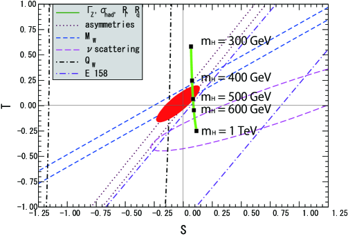
Figure 4: $S$ and $T$ plot: Contours show $1\sigma$ constraints (39.35 %) from various inputs except for the central one representing 90% CL allowed by all data [28].

We plot the parameters in a region of $300\,\text{GeV}\leq m_{H}\leq 1\,\text{TeV}$, and take the reference Higgs mass as 117 GeV. We find that the first KK Higgs mass $m_{H}=m_{KK}$ is constrained in the range $430\,\text{GeV}\lesssim m_{H}\lesssim 500\,\text{GeV}$ within 90% CL. Our plot roughly corresponds a diagonal line $m_{H}=1/R$ in Fig. 3 of Ref. [2], which gives $370\,\text{GeV}\lesssim m_{H}=1/R\lesssim 550\,\text{GeV}$ within 90% CL from the data 2002.

3.4 Dark matter

We comment on a dark matter (DM) candidate in our model. In the UED model, the lightest KK particle (LKP) can be a candidate for the DM because the KK parity is always conserved. The possibility that the KK photon becomes the LKP, and thus the DM candidate, has been widely discussed in a lot of literatures (see e.g. [29] for review and references).

If there is a reflection symmetry for the BCs in this scenario, the KK parity is conserved, and thus the LKP with odd ($n=1$) parity is stable, which can be a DM candidate. The masses of $n$th KK excitation states, $X^{(n)}$, of SM field are given by

$$m_{X^{(n)}}^{2}=n^{2}m_{KK}^{2}+m_{X^{(0)}}^{2},$$ (74)

at tree level, where $X^{(0)}$ and $m_{X^{(0)}}$ indicate the corresponding SM field and its mass. The mass of the neutral Higgs can be rewritten as

$$m_{H^{(n)}}^{2}=m_{H^{(n)}}^{2}+\delta m_{H^{(n)}}^{2},$$ (75)

including the radiative corrections to the KK masses induced from loop diagrams traversing around the extra dimension. On the other hand, the correction to the KK photon is given by [30]

$$\delta m_{A^{(n)}}^{2} = \frac{1}{2}\Bigg{[}\delta m_{B^{(n)}}^{2}+\delta m_{W^{(n)}}^{2}+\frac{1}{2}(g^{2}+g^{\prime}{}^{2})v_{\text{EW}}^{2}$$ (76)

$$\phantom{\frac{1}{2}\Bigg{[}}+\sqrt{\left\{\delta m_{B^{(n)}}^{2}-\delta m_{W^{(n)}}^{2}+\frac{1}{2}(g^{2}+g^{\prime}{}^{2})v_{\text{EW}}^{2}\right\}^{2}-(2gg^{\prime}v_{\text{EW}}^{2})^{2}}\Bigg{]},$$

where

$$\delta m_{B^{(n)}}^{2} = -\frac{39}{2}\frac{g^{\prime}{}^{2}\zeta(3)}{16\pi^{4}}m_{KK}^{2}-\frac{1}{3}\frac{g^{\prime}{}^{2}}{16\pi^{2}}n^{2}m_{KK}^{2}\ln\frac{\Lambda}{nm_{KK}},$$ (77)

$$\delta m_{W^{(n)}}^{2} = -\frac{5}{2}\frac{g^{2}\zeta(3)}{16\pi^{4}}m_{KK}^{2}+15\frac{g^{2}}{16\pi^{2}}n^{2}m_{KK}^{2}\ln\frac{\Lambda}{nm_{KK}}.$$ (78)

It is found that the LKP in our scenario is the KK photon naively since the mass of KK photon is similar to the UED case and further the Higgs mass does not aquire negative contribution from the quartic coupling as in UED.

3.5 FCNC problem

Finally, let us comment that our setup does not suffer from serious flavor changing neutral currents (FCNCs) problem since the model have only one Higgs doublet. We note that in our scenario, all the bulk fermions have a flat wave-function profile at the tree level where the bulk and brane Higgs potentials are not generated via renormalization group running. Therefore there are no tree level FCNC processes coming from the overlap integral along the extra-dimension. This is not affected by the fact that Higgs VEV and physical field have different profile. One might think that contribution from a loop of charged KK Higgs field is different from that in the UED model. However, the only difference is coming from the change of the BC from Neumann to Dirichlet. Therefore, the overlap integral of two $n$th-modes and a single (flat) zero-mode are identical in these two models, giving the same coupling. FCNC loop contributions from KK-modes are not different from the ordinary UED model [31]-[33].

3.6 Comparison of models

At the end of section, we tabulate phenomenological results of our model in comparison with other extra-dimensional models [10]. The models proposed in ref [10] have been considered in flat 5D spacetime with brane localized Higgs potential (BLP). The models of BLP have been classified into the BLF case and bulk fermion (BF) case, the latter corresponding to a more general setup of the UED model. We refer to the models given in [10] as BLP(BLF) and BLP(BF) in this subsection. The phenomenological aspects of our model and comparisons of it with BLP(BLF) and BLP(BF) scenarios are given in Table 2.

	BLP(BLF)	BLP(BF)
Top Yukawa	Tiny in small $\hat{\lambda}$	Tiny in $\hat{\lambda}$
deviation	$90\%$ in large $\hat{\lambda}$	$8\%$ in large $\hat{\lambda}$
$H^{(0)}$ production	Same as SM in small $\hat{\lambda}$	Same as SM in small $\hat{\lambda}$
by $gg$ fusion	$1\%$ of SM in large $\hat{\lambda}$	$85\%$ of SM in large $\hat{\lambda}$
$H^{(0)}$ production	Same as SM in small $\hat{\lambda}$	Same as SM in small $\hat{\lambda}$
by $WW$ fusion	$85\%$ of SM in large $\hat{\lambda}$	$85\%$ of SM in large $\hat{\lambda}$
$H^{(n)}$ production		$q^{(2n)}\bar{q}^{(2m)}\rightarrow H^{(2(l+1))}$
by $gg$ fusion	$q^{(n+1)}\bar{q}^{(m+1)}\rightarrow H^{(l+1)}$ in small $\hat{\lambda}$	$q^{(2n)}\bar{q}^{(2m+1)}\rightarrow H^{(2l+1)}$
		$q^{(2n+1)}\bar{q}^{(2m+1)}\rightarrow H^{(2(l+1))}$
$H^{(n)}$ production	$W^{(2n)}W^{(2m)}\rightarrow H^{(2(l+1))}$	$W^{(2n)}W^{(2m)}\rightarrow H^{(2(l+1))}$
by $WW$ fusion	$W^{(2n)}W^{(2m+1)}\rightarrow H^{(2l+1)}$	$W^{(2n)}W^{(2m+1)}\rightarrow H^{(2l+1)}$
	$W^{(2n+1)}W^{(2m+1)}\rightarrow H^{(2(l+1))}$	$W^{(2n+1)}W^{(2m+1)}\rightarrow H^{(2(l+1))}$
	$Z^{(2n)}\rightarrow Z^{(2m)}H^{(2(l+1))}$
Associated $H^{(n)}$	$Z^{(2n)}\rightarrow Z^{(2m+1)}H^{(2l+1)}$	$Z^{(0)}\rightarrow Z^{(2m)}H^{(2(l+1))}$
Production	$Z^{(2n+1)}\rightarrow Z^{(2m)}H^{(2l+1)}$	$Z^{(0)}\rightarrow Z^{(2m+1)}H^{(2l+1)}$
	$Z^{(2n+1)}\rightarrow Z^{(2m+1)}H^{(2(l+1))}$
KK parity	$\times$	$\bigcirc$
Dark matter	$\times$	$\bigcirc$
	Our Model
Top Yukawa	$10\%$
deviation
$H^{(0)}$ production	$81\%$ of SM
by $gg$ fusion
$H^{(0)}$ production	$81\%$ of SM
by $WW$ fusion
	$q^{(2n)}\bar{q}^{(2|n-l-1|)}\rightarrow H^{(2(l+1))}$
$H^{(n)}$ production	$q^{(2n)}\bar{q}^{(2|n-l|+1)}\rightarrow H^{(2l+1)}$
by $gg$ fusion	$q^{(2n+1)}\bar{q}^{(2|n-l|)}\rightarrow H^{(2l+1)}$
	$q^{(2n+1)}\bar{q}^{(|2(n-l)-1|)}\rightarrow H^{(2(l+1))}$
	$W^{(2n)}W^{(2|n-l-1|)}\rightarrow H^{(2(l+1))}$
$H^{(n)}$ production	$W^{(2n)}W^{(2|n-l|+1)}\rightarrow H^{(2l+1)}$
by $WW$ fusion	$W^{(2n+1)}W^{(2|n-l|+1)}\rightarrow H^{(2l+1)}$
	$W^{(2n+1)}W^{(|2(n-l)-1|)}\rightarrow H^{(2(l+1))}$
Associated $H^{(n)}$	$Z^{(0)}\rightarrow Z^{(l)}H^{(l)}$
Production
KK parity	$\bigcirc$
Dark matter	$\bigcirc$

Table 2: Comparisons of phenomenological consequences of our model with BLP models presented in [10]. Our model and BLP(BF) model have a reflection symmetry. ”81% of SM” means the ratio of the production cross section. And, the $\hat{\lambda}$ is a quartic coupling of Higgs in the brane localized potential.

Finally, we comment on the KK masses including the radiative corrections and LKP as DM candidate in the BLP(BF) model. The radiative corrections for the neutral KK Higgs (75) can be estimated as

$$\delta m_{H^{(n)}}^{2}\simeq\frac{n^{2}m_{KK}^{2}}{16\pi^{2}}\left(3g^{2}+\frac{3}{2}g^{\prime}{}^{2}-\hat{\lambda}\right)\ln\frac{\Lambda}{nm_{KK}}+\bar{m}_{H}^{2},$$ (79)

where $\hat{\lambda}$ and $\bar{m}_{H}$ indicate the Higgs quartic coupling and boundary mass term. Since the mass of KK photon including the radiative correction is the same as one of the UED and the model discussed in this paper, the KK photon becomes the LKP as the DM candidate in the BLP(BF) model as long as the reliable Higgs quartic coupling and boundary mass term are taken.

4 Summary

We have studied the 5D model where the all SM fields exist in the 5D bulk compactified on the line segment with the flat metric. The wave-function profiles of the Higgs and gauge fields have been presented under the Dirichlet BC for the Higgs and the Neumann BC for the gauge fields on the branes. It has been shown that a sufficiently flat profile of the longitudinal component of the zero-mode gauge boson can be obtained by a superposition of the KK-mode of NG bosons.

We have also presented phenomenological discussions on the top Yukawa deviation, the production and decay of Higgs, constraints on the model from the EW precision measurements, and dark matter candidate. In the model, the top Yukawa deviation of 10% is predicted. The cross section for the Higgs production, such as the gluon and $WW$ fusions, in this model are over all decreased to 81% of the SM expectations. Therefore, the branching ratios are not changed. For the Higgs decay, the width of the process $H\rightarrow WW$, which is the dominant one, is as large as the Higgs mass. The evaluation of the $S$ and $T$ parameters suggests that the KK scale of $430\mbox{ GeV}\lesssim m_{H}\lesssim 500\mbox{ GeV}$ is favored in this scenario.

Acknowledgments

We are grateful to T. Yamashita for very helpful discussions and thank S. Matsumoto for useful comments. This work is partially supported by Scientific Grant by Ministry of Education and Science, Nos. 20540272, 20039006, 20025004, 20244028, and 19740171. The work of RT is supported by the DFG-SFB TR 27.

Appendix

Gauge Fixing

We give our notation with 5D Higgs kinetic Lagrangian and gauge fixing in this Appendix. In our notation, the VEV and quantum fluctuation are given by

$$\Phi^{c}(x,z) = \left(\begin{array}[]{c}0\\ v\end{array}\right),$$ (82)

$$\Phi^{q}(x,z) = \left(\begin{array}[]{c}\varphi^{+}(x,z)\\ \frac{1}{\sqrt{2}}[H(x,z)+i\chi(x,z)]\end{array}\right)=\left(\begin{array}[]{c}\displaystyle\sum_{n=0}^{\infty}f_{n}^{\varphi^{+}}(z)\varphi_{n}^{+}(x)\\ \frac{1}{\sqrt{2}}\displaystyle\sum_{n=0}^{\infty}[f_{n}^{H}(z)H_{n}(x)+if_{n}^{\chi}(z)\chi_{n}(x)]\end{array}\right).$$ (87)

The covariant derivative on the Higgs field is written down as

$$D_{M}\Phi = \partial_{M}\Phi+\frac{ig_{5}}{\sqrt{2}}\left(\begin{array}[]{cc}0&W_{M}^{+}\\ W_{M}^{-}&0\end{array}\right)\Phi+ie\left(\begin{array}[]{cc}\frac{1}{\tan 2\theta_{W}}Z_{M}+A_{M}&0\\ 0&-\frac{1}{\sin 2\theta_{W}}Z_{M}\end{array}\right)\Phi$$ (92)

$$= \left(\begin{array}[]{c}\partial_{M}\varphi^{+}\\ \frac{\partial_{M}H+i\partial_{M}\chi}{\sqrt{2}}\end{array}\right)+\frac{ig_{5}}{\sqrt{2}}\left(\begin{array}[]{c}W_{M}^{+}\left(v+\frac{H+i\chi}{\sqrt{2}}\right)\\ W_{M}^{-}\varphi^{+}\end{array}\right)+ie_{5}\left(\begin{array}[]{c}\left(\frac{1}{\tan 2\theta_{W}}Z_{M}+A_{M}\right)\varphi^{+}\\ -\frac{1}{\sin 2\theta_{W}}Z_{M}\left(v+\frac{H+i\chi}{\sqrt{2}}\right)\end{array}\right),$$ (99)

where the gauge fields are defined in Eq.(34), and $e_{5}\equiv g_{5}g_{5}^{\prime}/\sqrt{g_{5}^{2}+{g_{5}^{\prime}}^{2}}$. Note that mass dimensions are $[g_{5}]=[g_{5}^{\prime}]=[e_{5}]=-1/2$ and $[v]=[W^{\pm}_{M}]=[Z_{M}]=[A_{M}]=3/2$. The Higgs kinetic Lagrangian is given by

$$\mathcal{L}_{H} =-\left|D_{M}\Phi\right|^{2}$$

$$=-\left|\partial_{M}\varphi^{+}+im_{W}W_{M}^{+}+{ig_{5}\over 2}W_{M}^{+}\left(H+i\chi\right)+ie_{5}\left({1\over\tan 2\theta_{W}}Z_{M}+A_{M}\right)\varphi^{+}\right|^{2}$$

$$\quad-{1\over 2}\left|\partial_{M}H+i\partial_{M}\chi+ig_{5}W_{M}^{-}\varphi^{+}-im_{Z}Z_{M}-{ie_{5}\over\sin 2\theta_{W}}Z_{M}\left(H+i\chi\right)\right|^{2}.$$

The quadratic terms are given by

$$\mathcal{L}_{H}^{\text{quad}} =-\left|\partial_{M}\varphi^{+}\right|^{2}-{\left(\partial_{M}H\right)^{2}+\left(\partial_{M}\chi\right)^{2}\over 2}-m_{W}^{2}\left|W_{M}^{+}\right|^{2}-{m_{Z}^{2}\over 2}(Z_{M})^{2}$$

$$\quad+im_{W}\left(W^{-M}\partial_{M}\varphi^{+}-W^{+M}\partial_{M}\varphi^{-}\right)+m_{Z}Z^{M}\partial_{M}\chi.$$

We employ the following $R_{\xi}$-$like$ gauge fixing

$$\mathcal{L}_{\text{GF}}=-f^{+}f^{-}-\frac{1}{2}(f^{Z}f^{Z}+f^{A}f^{A}),$$

where

$$f^{\pm} \equiv\frac{1}{\sqrt{\xi_{W}}}\left(\partial_{M}W^{\pm M}\mp i\xi_{W}m_{W}\varphi^{\pm}\right),$$

$$f^{Z} \equiv\frac{1}{\sqrt{\xi_{Z}}}\left(\partial_{M}Z^{M}-\xi_{Z}m_{Z}\chi\right),$$

$$f^{A} \equiv\frac{1}{\sqrt{\xi_{A}}}\partial_{M}A^{M}.$$

Now, we can write down as

$$\mathcal{L}_{\text{GF}} =-{1\over\xi_{W}}\left|\partial_{M}W^{+M}\right|^{2}-{1\over 2\xi_{Z}}\left(\partial_{M}Z^{M}\right)^{2}-{1\over 2\xi_{A}}\left(\partial_{M}A^{M}\right)^{2}$$

$$\quad+im_{W}\left(\varphi^{+}\partial_{M}W^{-M}-\varphi^{-}\partial_{M}W^{+M}\right)+m_{Z}\chi\partial_{M}Z^{M}-\xi_{W}m_{W}^{2}\left|\varphi^{+}\right|^{2}-{\xi_{Z}m_{Z}^{2}\over 2}\chi^{2}.$$

The sum of quadratic terms from Higgs kinetic Lagrangian and gauge fixing terms are given by

$$\mathcal{L}_{H+\text{GF}}^{\text{quad}} =-\left|\partial_{M}\varphi^{+}\right|^{2}-\xi_{W}m_{W}^{2}\left|\varphi^{+}\right|^{2}-{1\over 2}\left(\partial_{M}\chi\right)^{2}-{\xi_{Z}m_{Z}^{2}\over 2}\chi^{2}-{1\over 2}\left(\partial_{M}h\right)^{2}$$

$$\quad-\frac{1}{\xi_{W}}\left|\partial_{N}W^{+N}\right|^{2}-m_{W}^{2}\left|W_{M}^{+}\right|^{2}-{1\over 2\xi_{Z}}\left(\partial_{N}Z^{N}\right)^{2}-{m_{Z}^{2}\over 2}(Z_{M})^{2}-{1\over 2\xi_{A}}\left(\partial_{M}A^{M}\right)^{2}$$

$$\quad+\partial_{5}\left[im_{W}\left(W^{-}_{5}\varphi^{+}-W^{+}_{5}\varphi^{-}\right)+m_{Z}Z_{5}\chi\right].$$

One can consider some specific gauge choices. Here, we comment on the ’t Hooft-Feynmann gauge ($\xi_{V}=1$, $V=W,Z,A$) and unitary gauge ($\xi_{V}\rightarrow\infty$). The above sum of quadratic terms can be simplified to be

$$\mathcal{L}_{H+\text{GF}_{\xi_{V}=1}}^{\text{quad}} =-\left|\partial_{M}\varphi^{+}\right|^{2}-m_{W}^{2}\left|\varphi^{+}\right|^{2}-{1\over 2}\left(\partial_{M}\chi\right)^{2}-{m_{Z}^{2}\over 2}\chi^{2}-{1\over 2}\left(\partial_{M}h\right)^{2}$$

$$\quad-\left|\partial_{N}W^{+N}\right|^{2}-m_{W}^{2}\left|W_{M}^{+}\right|^{2}-{1\over 2}\left(\partial_{N}Z^{N}\right)^{2}-{m_{Z}^{2}\over 2}(Z_{M})^{2}-{1\over 2}\left(\partial_{M}A^{M}\right)^{2}$$

$$\quad+\partial_{5}\left[im_{W}\left(W^{-}_{5}\varphi^{+}-W^{+}_{5}\varphi^{-}\right)+m_{Z}Z_{5}\chi\right].$$

in the ’t Hooft-Feynmann gauge, and

$$\mathcal{L}_{H+\text{GF}_{\xi_{V}\rightarrow\infty}}^{\text{quad}}\rightarrow-{1\over 2}\left(\partial_{M}h\right)^{2}-m_{W}^{2}\left|W_{M}^{+}\right|^{2}-{m_{Z}^{2}\over 2}(Z_{M})^{2},$$

in the unitary gauge. Notice that unphysical degrees of freedom, that is, the would-be NG bosons $\varphi^{\pm}$ and $\chi$, become infinitely heavy and decouple.

Finally, let us give the gauge kinetic Lagrangian in the ’t Hooft-Feynmann gauge. The gauge kinetic Lagrangian is written by

$$\mathcal{L}_{\text{YM}} =-{1\over 4}\left(\sum_{a=1}^{3}F^{a}_{MN}F^{aMN}+F^{B}_{MN}F^{B\,MN}\right).$$

By utilizing the following redefinition,

$$F^{\pm}_{MN} =\partial_{M}W^{\pm}_{N}-\partial_{N}W^{\pm}_{M}\pm 2ig\left(W_{M}^{3}W^{\pm}_{N}-W_{N}^{3}W_{M}^{\pm}\right),$$

$$F^{3}_{MN} =\partial_{M}W^{3}_{N}-\partial_{N}W^{3}_{M}+2g\left(W^{+}_{M}W^{-}_{N}-W^{+}_{N}W^{-}_{M}\right),$$

with $W^{3}_{M}=cZ_{M}+sA_{M}$, we can rewrite

$$\mathcal{L}_{\text{YM}} =-{1\over 2}F^{+}_{MN}F^{-MN}-{1\over 4}\left[F^{3}_{MN}F^{3\,MN}+F^{B}_{MN}F^{B\,MN}\right].$$

Therefore, quadratic terms are

$$\mathcal{L}_{\text{YM}}^{\text{quad}} =-{1\over 2}\sum_{a=1}^{3}\left(-W^{a}_{\mu}\Box W^{a\mu}-\left(\partial_{\mu}W^{a\mu}\right)^{2}+\left(\partial_{5}W^{a}_{\mu}\right)\left(\partial_{5}W^{a\mu}\right)-W_{5}^{a}\Box W_{5}^{a}\right.$$

$$\left.\hskip 281.6821pt+2W_{5}^{a}\partial_{5}\left(\partial_{\mu}W^{a\mu}\right)\right)$$

$$\quad-{1\over 2}\left(-B_{\mu}\Box B^{\mu}-\left(\partial_{\mu}B^{\mu}\right)^{2}+\left(\partial_{5}B_{\mu}\right)\left(\partial_{5}B^{\mu}\right)-B_{5}\Box B_{5}+2B_{5}\partial_{5}\left(\partial_{\mu}B^{\mu}\right)\right)$$

$$=-\left[-W^{+}_{\mu}\Box W^{-\mu}-\left|\partial_{\mu}W^{+\mu}\right|^{2}+\left(\partial_{5}W^{+}_{\mu}\right)\left(\partial_{5}W^{-\mu}\right)\right]$$

$$\quad-\left[-W_{5}^{+}\Box W_{5}^{-}+W_{5}^{+}\partial_{5}\left(\partial_{\mu}W^{-\mu}\right)+W_{5}^{-}\partial_{5}\left(\partial_{\mu}W^{+\mu}\right)\right]$$

$$\quad-{1\over 2}\left(-Z_{\mu}\Box Z^{\mu}-\left(\partial_{\mu}Z^{\mu}\right)^{2}+\left(\partial_{5}Z_{\mu}\right)\left(\partial_{5}Z^{\mu}\right)-Z_{5}\Box Z_{5}+2Z_{5}\partial_{5}\left(\partial_{\mu}Z^{\mu}\right)\right)$$

$$\quad-{1\over 2}\left(-A_{\mu}\Box A^{\mu}-\left(\partial_{\mu}A^{\mu}\right)^{2}+\left(\partial_{5}A_{\mu}\right)\left(\partial_{5}A^{\mu}\right)-A_{5}\Box A_{5}+2A_{5}\partial_{5}\left(\partial_{\mu}A^{\mu}\right)\right).$$

References

- [1] T. Appelquist, H. C. Cheng and B. A. Dobrescu, Phys. Rev. D 64 (2001) 035002, [arXiv:hep-ph/0012100].
- [2] T. Appelquist and H. U. Yee, Phys. Rev. D 67, 055002 (2003), [arXiv:hep-ph/0211023].
- [3] I. Gogoladze and C. Macesanu, Phys. Rev. D 74, 093012 (2006), [arXiv:hep-ph/0605207].
- [4] P. Nath and M. Yamaguchi, Phys. Rev. D 60, 116004 (1999), [arXiv:hep-ph/9902323].
- [5] M. Masip and A. Pomarol, Phys. Rev. D 60, 096005 (1999), [arXiv:hep-ph/9902467].
- [6] T. G. Rizzo and J. D. Wells, Phys. Rev. D 61, 016007 (2000), [arXiv:hep-ph/9906234].
- [7] A. Strumia, Phys. Lett. B 466, 107 (1999), [arXiv:hep-ph/9906266].
- [8] C. D. Carone, Phys. Rev. D 61, 015008 (2000), [arXiv:hep-ph/9907362].
- [9] K. m. Cheung and G. L. Landsberg, Phys. Rev. D 65 (2002) 076003, [arXiv:hep-ph/0110346].
- [10] N. Haba, K. Oda and R. Takahashi, Nucl. Phys. B 821 (2009) 74, [Erratum-ibid. 824 (2010) 331], [arXiv:0904.3813 [hep-ph]].
- [11] N. Haba, K. Oda and R. Takahashi, arXiv:0910.4528 [hep-ph].
- [12] N. Haba, K. Oda and R. Takahashi, arXiv:0910.3356 [hep-ph].
- [13] Y. Hosotani and Y. Kobayashi, Phys. Lett. B 674, 192 (2009), [arXiv:0812.4782 [hep-ph]].
- [14] M. Holthausen and R. Takahashi, arXiv:0912.2262 [hep-ph].
- [15] L. J. Hall, H. Murayama and Y. Nomura, Nucl. Phys. B 645 (2002) 85, [arXiv:hep-th/0107245].
- [16] R. S. Chivukula, D. A. Dicus and H. J. He, Phys. Lett. B 525, 175 (2002), [arXiv:hep-ph/0111016].
- [17] R. S. Chivukula and H. J. He, Phys. Lett. B 532, 121 (2002), [arXiv:hep-ph/0201164].
- [18] Y. Abe, N. Haba, Y. Higashide, K. Kobayashi and M. Matsunaga, Prog. Theor. Phys. 109 (2003) 831, [arXiv:hep-th/0302115].
- [19] R. S. Chivukula, D. A. Dicus, H. J. He and S. Nandi, Phys. Lett. B 562 (2003) 109, [arXiv:hep-ph/0302263].
- [20] C. Csaki, C. Grojean, H. Murayama, L. Pilo and J. Terning, Phys. Rev. D 69 (2004) 055006, [arXiv:hep-ph/0305237].
- [21] Y. Abe, N. Haba, K. Hayakawa, Y. Matsumoto, M. Matsunaga and K. Miyachi, Prog. Theor. Phys. 113, 199 (2005), [arXiv:hep-th/0402146].
- [22] N. Haba, Y. Sakamura and T. Yamashita, JHEP 0907, 020 (2009), [arXiv:0904.3177 [hep-ph]]; JHEP 1003, 069 (2010), [arXiv:0908.1042 [hep-ph]].
- [23] ATLAS Collaborations, CERN/LHCC/99-15 (1999).
- [24] G. L. Bayatian et al. [CMS Collaboration], J. Phys. G 34 (2007) 995.
- [25] M. E. Peskin and T. Takeuchi, Phys. Rev. Lett. 65 (1990) 964.
- [26] M. E. Peskin and T. Takeuchi, Phys. Rev. D 46 (1992) 381.
- [27] D. C. Kennedy and B. W. Lynn, Nucl. Phys. B 322 (1989) 1.
- [28] C. Amsler et al. (Particle Data Group), Phys. Lett. B 667 (2008) 1.
- [29] D. Hooper and S. Profumo, Phys. Rept. 453 (2007) 29, [arXiv:hep-ph/0701197].
- [30] H. C. Cheng, K. T. Matchev and M. Schmaltz, Phys. Rev. D 66 (2002) 036005, [arXiv:hep-ph/0204342].
- [31] A. J. Buras, A. Poschenrieder, M. Spranger and A. Weiler, [arXiv:hep-ph/0307202].
- [32] R. Mohanta and A. K. Giri, Phys. Rev. D 75 (2007) 035008, [arXiv:hep-ph/0611068].
- [33] P. Colangelo, F. De Fazio, R. Ferrandes and T. N. Pham, Phys. Rev. D 77 (2008) 055019, [arXiv:0709.2817 [hep-ph]].