Context models on sequences of covers

Abstract

We present a class of models that, via a simple construction, enables exact, incremental, non-parametric, polynomial-time, Bayesian inference of conditional measures. The approach relies upon creating a sequence of covers on the conditioning variable and maintaining a different model for each set within a cover. Inference remains tractable by specifying the probabilistic model in terms of a random walk within the sequence of covers. We demonstrate the approach on problems of conditional density estimation, which, to our knowledge is the first closed-form, non-parametric Bayesian approach to this problem.

1 Introduction

Conditional measure estimation is a fundamental problem in statistics. Specific instances of this problem include classification, regression and conditional density estimation. This paper formulates a general approach for non-parametric, incremental, closed-form Bayesian estimation of conditional measures that relies on a model structure defined on a sequence of covers. This is an important development, particularly for the problem of conditional density estimation, where although non-parameteric kernel-based approaches that currently dominate generally perform well, a fast, tractable, incremental, Bayesian approach has been lacking.

This construction used in this paper employs a random walk in a set of contexts. In its simplest form, this can be seen as a descendant of context tree methods for variable order Markov models (Willems et al., 1995; Dimitrakakis, 2010) and Bayesian non-parametric methods for tree-based density estimation approaches (Hutter, 2005; Wong and Ma, 2010). These approaches utilise a stopping variable construction on a tree to simplify inference. The central contribution of this paper is to generalise this to a terminating random walk on a lattice. Then the inference procedure remains tractable, while the lattice structure increases the flexibility and applicability of the model. As an example, the proposed framework is applied to the important problem of conditional density estimation, obtaining the first closed-form, incremental, non-parametric Bayesian approach to this problem.

Stated generally, the problem of incremental, conditional measure estimation in a Bayesian setting is as follows. We observe the sequences $x^{t}=\left(x_{i}\mathrel{:}i=1,\ldots,t\right)$ and $y^{t}=\left(y_{i}\mathrel{:}i=1,\ldots,t\right)$, with $x_{i}\in{\mathcal{X}}$ and $y_{i}\in{\mathcal{Y}}$. Informally, our goal is the prediction of the next observation $y_{t+1}$ given the next conditioning variable $x_{t+1}$ and all previous evidence $x^{t},y^{t}$. More precisely, we wish to calculate the probability measure:

$$\psi_{t}(Y\mid x_{t+1})\mathrel{\triangleq}\mathop{\mbox{$\mathbb{P}$}}\nolimits(y_{t+1}\in Y\mid x^{t+1},y^{t})$$ (1)

for all $Y\in{\mathfrak{B}}_{{\mathcal{Y}}}$, where ${\mathfrak{B}}_{{\mathcal{Y}}}$ denotes the Borel sets of ${\mathcal{Y}}$, through Bayes’ theorem.

The main idea we use to tackle this problem is to first define a sequence of covers on the space of all sequences $x^{t}$. Each cover is a collection of sets, such that for any sequence $x^{t}$ there exists at least one set $c$ in every cover containing that sequence. In addition, each set $M$ corresponds to a model $\phi_{M}$ on ${\mathcal{Y}}$. In order to combine these, we introduce a random variable $S_{t}\in{\mathscr{C}}$, such that $\xi_{t}(M\mid x_{t+1})\mathrel{\triangleq}\mathop{\mbox{$\mathbb{P}$}}\nolimits(S_{t}=M\mid x^{t+1},y^{t})$, is the probability of the model $\phi_{M}$. Then the conditional measure:

$$\psi_{t}(Y\mid x_{t+1})=\sum_{M\in{\mathscr{C}}}\phi_{M}^{t}(Y\mid x_{t+1})\xi_{t}(M\mid x_{t+1}),$$ (2)

can be readily obtained via marginalisation over the set of contexts.

We show that via the sequence of covers, $\xi$ can be specified in terms of a random walk. This allows closed-form, incremental inference to be performed in polynomial time for conditional densitiy estimation and variable order Markov models, by selecting the covers appropriately. The resulting class of models allows the introduction of several other interesting model classes.

2 Context models

We first introduce some notation and basic assumptions. Unless otherwise stated, we assume that all sets ${\mathcal{X}}$ are measurable with respect to some $\sigma$-algebra ${\mathfrak{B}}_{{\mathcal{X}}}$. We denote sequences of observations $x_{i}\in{\mathcal{X}}$ by $x^{t}\mathrel{\triangleq}\left(x_{i}\mathrel{:}i=1,\ldots,t\right)$. The set ${\mathcal{X}}^{0}\mathrel{\triangleq}\left\{\mathbf{0}\right\}$ contains only the null sequence $\mathbf{0}$, while ${\mathcal{X}}^{n}\mathrel{\triangleq}\times^{n}{\mathcal{X}}$ denotes the sequences of length $n$ and the set of all sequences is denoted by ${\mathcal{X}}^{*}\mathrel{\triangleq}\bigcup_{n=0}^{\infty}{\mathcal{X}}^{n}$. Finally, we denote the length of any sequence $x\in{\mathcal{X}}^{*}$ by $\ell\left(x\right)$ such that $x\in{\mathcal{X}}^{\ell\left(x\right)}$.

A cover ${\mathcal{C}}$ of some set $A$ is a collection of sets such that $\bigcup_{M\in C}M\supset A$. A refinement ${\mathcal{C}}^{\prime}$ of ${\mathcal{C}}$ is a cover of $A$ such that for any $M^{\prime}\in{\mathcal{C}}^{\prime}$, there is some $M\in{\mathcal{C}}$ such that $M^{\prime}\subset M$. We consider models constructed on a sequence of covers $\mathfrak{C}\mathrel{\triangleq}\left({\mathcal{C}}_{k}\mathrel{:}k=1,\ldots\right)$ of ${\mathcal{X}}^{*}$. Letting ${\mathscr{C}}\mathrel{\triangleq}\bigcup_{k}{\mathcal{C}}_{k}$ be the collection of all subsets in our sequence of covers, we refer to each subset $M\in{\mathcal{C}}$ as a context. Partition trees, where each cover is disjoint and a refinement of the previous cover, are an interesting special case:

Example 1 (Binary alphabet).

Let ${\mathcal{X}}=\left\{0,1\right\}$. For $k=1,2,\ldots$, let ${\mathcal{C}}_{k}$ be the partition of ${\mathcal{X}}^{*}$ into $2^{k-1}$ subsets, with the following property. For all $M\in{\mathcal{C}}_{k}$, and any $a,b\in{\mathcal{X}}^{*}$: $a,b\in M$ if and only if $a_{\ell\left(a\right)-i}=b_{\ell\left(b\right)-i}$ for all $i=0,\ldots,k-1$. This creates a sequence of partitions based on a suffix tree and can be used in the development of variable order Markov models.

Example 2 (Unit interval).

Let ${\mathcal{X}}=[0,1]$. For $k=1,2,\ldots$, let ${\mathcal{C}}_{k}$ be the partition of ${\mathcal{X}}^{*}$ into $2^{k-1}$ subsets, $M_{k,i}\mathrel{\triangleq}\left\{x\in{\mathcal{X}}^{*}\mathrel{:}x_{\ell\left(x\right)}\in[2^{k-1}(i-1),2^{k-1}i)\right\}$. A generalised form of this sequence of covers is used in the construction of conditional density estimation using the proposed construction, and shall be the main focus of the current paper.

We now describe a conditional measure on ${\mathcal{Y}}$ indexed by ${\mathcal{X}}^{*}$ defined on such a structure. This will form the basis for conditional measure estimation. Intuitively, the structure defines a set of probability measures on ${\mathcal{Y}}$, indexed by the set of all contexts. The structure is such that, for any $x\in{\mathcal{X}}$ there is only one corresponding context $f(x)$, even if there are many contexts containing $x$. The contexts themselves have the property that the corresponding context for any $x$ in the set they define is either the same context or one of the subsequent contexts in the sequence of covers. This will be useful later, since it will allow us to perform closed form inference on a distribution of context models.

Definition 1.

A context model $\mu=({\mathcal{P}},f)$ defined on a (countable) sequence of covers $\mathfrak{C}=\left({\mathcal{C}}_{k}\mathrel{:}k=1,\ldots,\right)$ of ${\mathcal{X}}^{*}$, is composed of:

1. A set ${\mathcal{P}}$ of “local” probability measures on ${\mathcal{Y}}$, conditional on ${\mathcal{X}}^{*}$ and indexed by elements in the set of contexts ${\mathscr{C}}=\bigcup_{k}{\mathcal{C}}_{k}$:

   $${\mathcal{P}} \mathrel{\triangleq}\left\{p_{M}(\cdot\mid x)\mathrel{:}M\in{\mathscr{C}}\right\}, x \in{\mathcal{X}}^{*}.$$ (3)

2. A context map $f:{\mathcal{X}}^{*}\to{\mathcal{C}}$ such that $\forall x\in{\mathcal{X}}^{*}$, if $f(x)\in{\mathcal{C}}_{k}$, then for any $x^{\prime}\in f(x)$ it holds that $f(x^{\prime})\cap f(x)\neq\emptyset$ and $f(x^{\prime})\in{\mathcal{C}}_{k+h}$ with $h\geq 0$.

The model $\mu$ specifies the following conditional measure on ${\mathcal{Y}}$ for any $x\in{\mathcal{X}}^{*}$:

$$\mathop{\mbox{$\mathbb{P}$}}\nolimits_{\mu}(Y\mid x) =p_{f(x)}(Y\mid x), Y \subset{\mathcal{Y}}.$$ (4)

Though the local measures ${\mathcal{P}}$ can be simple, so that inference can be efficient, the model’s overall complexity will depend on the context map and cover structure.

We now describe a distribution of such models, whereby exact Bayesian inference can be performed in polynomial time. Intuitively, the distribution can be seen as a two-stage process. Firstly, we sample a context map $f$ from a set of context maps ${\mathcal{F}}$, through a halting random walk on the set of all contexts. Secondly, for each context $M$ we sample a conditional measure $p_{M}$ from a distribution $\phi_{M}$. The construction of and sampling from this distribution, are discussed in Sec.2.1, while Sec. 2.2 shows how to sample from marginal distribution $\psi$ and Sec. 2.3 derives the inference procedure.

2.1 Construction of the context model distribution

Definition 2 (Cover model).

A cover model defines a distributilateon $\xi$ on context models $\mu=({\mathcal{P}},f)$, through a tuple $(\mathfrak{C},{\mathcal{W}},{\mathcal{V}},\Phi)$, where:

1. $\mathfrak{C}\mathrel{\triangleq}\left({\mathcal{C}}_{k}\mathrel{:}k=1,\ldots\right)$ is a sequence of covers, and ${\mathscr{C}}\mathrel{\triangleq}\left\{M\in{\mathcal{C}}\mathrel{:}{\mathcal{C}}\in\mathfrak{C}\right\}$ is the set of all contexts in each cover.

2. ${\mathcal{W}}=\left\{w_{M}\mathrel{:}M\in{\mathscr{C}}\right\}$, with $w_{M}\in[0,1]$, is a set of stopping probabilities.

3. ${\mathcal{V}}=\left\{v_{M}\mathrel{:}M\in{\mathscr{C}}\right\}$ is a set of transition probability vectors, such that: $\|v_{M}\|_{1}=1$, and that if $M\in{\mathcal{C}}_{k}$, then $v_{M,N}\in[0,1]$ for all $N\in{\mathcal{C}}_{k-1}$ such that $N\cap M\neq\emptyset$ while $v_{M,N}=0$ otherwise

4. $\Phi=\left\{\phi_{M}\mathrel{:}M\in{\mathscr{C}}\right\}$, is a set of priors such that each $\phi_{M}$ is a probability measure on ${\mathfrak{D}}_{{\mathcal{Y}}\mid{\mathcal{X}}}$, where ${\mathfrak{D}}_{{\mathcal{Y}}\mid{\mathcal{X}}}\mathrel{\triangleq}\left\{p_{\theta}(\cdot\mid x)\mathrel{:}\theta\in\Theta\right\}$ is a set of probability measures on ${\mathcal{Y}}$, conditional on $x\in{\mathcal{X}}$ and parameterised in $\Theta$.

In order to sample a context model $\mu=({\mathcal{P}},f)$ from $\xi=(\mathfrak{C},{\mathcal{W}},{\mathcal{V}},\Phi)$, we draw ${\mathcal{P}}$ directly from $\Phi$, while we construct $f$ via two auxiliary variables $\widehat{w_{M}},\widehat{v_{M}}$ drawn respectively from a Bernoulli and a multinomial distribution:

$$p_{M} \sim\phi_{M}$$ (5a)

$$\widehat{w_{M}} \sim{\mathpzc{Bern}}(w_{M})$$ (5b)

$$\widehat{v_{M}} \sim{\mathpzc{Mult}}(v_{M}).$$ (5c)

These draws are performed independently for all $M\in{\mathscr{C}}$. The construction of $f$ relies on the cover structure. For any $x^{t}\in{\mathcal{X}}^{*}$, we denote the collection of contexts at depth $k$ containing $x^{t}$ by

$${\mathcal{C}}_{k}^{t} \mathrel{\triangleq}\left\{M\in{\mathcal{C}}_{k}\mathrel{:}x^{t}\in M\right\}.$$ (6)

We then define the context map $f$ as follows: $f(x^{t})=M\in{\mathcal{C}}_{k}^{t}$, if and only if $\widehat{w_{M}}=1$ and $\widehat{w_{N}}=0$ for all $N\in{\mathcal{C}}_{h}^{t}$ with $h<k$.

2.2 Drawing samples from the marginal distribution

In order to generate an observation in ${\mathcal{Y}}$ from the marginal distribution derived from $\xi$, we can perform the following random walk.

Definition 3 (Marginal samples).

We perform a random walk on the sequence of covers $\mathfrak{C}=\left({\mathcal{C}}_{k}\mathrel{:}k=1,\ldots,0pt\right)$, with parameters ${\mathcal{W}},{\mathcal{V}}$, generates a random sequence $S_{1},\ldots,S_{K}$, with $K\in\left\{1,\ldots,0pt\right\}$, such that at each stage $k$,

1. $S_{k}\in{\mathcal{C}}_{0pt+1-k}$ for all $k$.

2. With probability $w_{S_{k}}$, the walk stops and we generate a local model $\phi$ from $\psi_{S_{k}}$ and subsequently an observation $x$ from $\phi$.

3. Otherwise, $S_{k+1}=N$ with probability $v_{S_{k},N}$, for all $N\in{\mathcal{C}}_{d+k}$.

2.3 Inference

At time $t$, we have observed $x^{t}=\left(x_{i}\mathrel{:}i=1,\ldots,t\right)$ and $y^{t}=\left(y_{i}\mathrel{:}i=1,\ldots,t\right)$ our model now has parameters ${\mathcal{W}}_{t},{\mathcal{V}}_{t}$, describing a distribution over context models. We wish to update these parameters in the light of new evidence $x_{t+1},y_{t+1}$. The main idea is to use a random walk that halts at some context $M_{t}$, in order to marginalise over context models. By definition, for any observation sequence, there is at least one context containing $x^{t}$ in every cover ${\mathcal{C}}_{k}$. We denote the collection of those contexts by ${\mathcal{C}}_{k}^{t}$, as in (6).

We start each stage $k$ of the walk at a context $S_{k}=N\in{\mathcal{C}}_{k}^{t}$ and proceed to $k-1,k-2,\ldots,1$. Let $B_{k}^{t}\mathrel{\triangleq}\left\{M_{t}\in\bigcup_{j=1}^{k}C^{t}_{j}\right\}$ denote the event that the walk stops in one of the first $k$ stages. Then, with probability $w_{M}^{t}$, we generate the next observation from the context $N\in{\mathcal{C}}_{k}^{t}$, so that $y_{t+1}\mid x^{t+1}\sim\phi_{N}^{t}(\cdot\mid x_{t+1})$. Otherwise, we proceed to the next stage, $k+1$, by moving to context $K\in C_{k+1}^{t}$ with probability $v^{t}_{N,K}$. More precisely:

$$v^{t}_{N,K} \mathrel{\triangleq}\mathop{\mbox{$\mathbb{P}$}}\nolimits(S_{k-1}=K\mid S_{k}=N,x^{t}),$$ (7)

$$w_{N}^{t} =\mathop{\mbox{$\mathbb{P}$}}\nolimits(M_{t}\in C_{k}\mid S_{k}=N,B^{t}_{k},x^{t}).$$ (8)

The central quantity for tractable inference in this model is the marginal prediction given the event $B_{k}^{t}$, for which we can obtain the following recursion:

$$\psi^{t}_{N}(y_{t+1}|x_{t+1})\mathrel{\triangleq}\mathop{\mbox{$\mathbb{P}$}}\nolimits(y_{t+1}|S_{k}{=}N,B^{t}_{k},x^{t+1})\\ =w_{N}^{t}\phi_{N}^{t}(y_{t+1}|x_{t+1})+(1-w_{N}^{t})\mathop{\mbox{$\mathbb{P}$}}\nolimits(y_{t+1}|S_{k}{=}N,B^{t}_{k-1},x^{t+1}),$$ (9)

noting that if we do not stop at level $k$ then $B^{t}_{k-1}$ is trivially true, or more precisely, if $B_{k}^{t}$ and $M_{t}\notin{\mathcal{C}}_{k}^{t}$ then $B_{k-1}^{t}$. Furthermore, it is easy to see that:

$$\mathop{\mbox{$\mathbb{P}$}}\nolimits(y_{t+1}\mid S_{k}=N,B^{t}_{k-1},x^{t+1}) =\sum_{\mathchoice{\hbox to0.0pt{\hss$\displaystyle{K\in{\mathcal{C}}_{k-1}^{t}}$\hss}}{\hbox to0.0pt{\hss$\textstyle{K\in{\mathcal{C}}_{k-1}^{t}}$\hss}}{\hbox to0.0pt{\hss$\scriptstyle{K\in{\mathcal{C}}_{k-1}^{t}}$\hss}}{\hbox to0.0pt{\hss$\scriptscriptstyle{K\in{\mathcal{C}}_{k-1}^{t}}$\hss}}}\psi_{K}^{t}(y_{t+1}\mid x_{t+1})v_{N,K}^{t}.$$ (10)

We can now calculate the stopping probabilities $w$ and the transition probabilities $v$ given the new evidence as follows:

Theorem 1.

Given a set of stopping parameters ${\mathcal{W}}_{t}=\left\{w_{M}^{t}\mathrel{:}M\in{\mathscr{C}}\right\}$, a set of transition parameters ${\mathcal{V}}_{t}=\left\{v_{K,N}^{t}\mathrel{:}K\in{\mathcal{C}}_{k},N\in{\mathcal{C}}_{k-1},k=1,\ldots\right\}$ and a set of local measures on ${\mathcal{X}}$: $\left\{\phi_{K}^{t}\mathrel{:}K\in{\mathscr{C}}\right\}$, then the parameters at the next time step are given by:

$$v^{t+1}_{N,K}=\frac{\psi_{N}^{t}(y_{t+1}\mid x_{t+1})v^{t}_{N,K}}{\sum_{M}\psi_{M}^{t}(x_{t+1})v^{t}_{M.K}}$$ (11)

and

$$w_{M}^{t+1}=\frac{\psi_{k}^{t}(y_{t+1}\mid x_{t+1})w_{M}^{t}}{\psi_{k}^{t}(y_{t+1}\mid x_{t+1})w_{M}^{t}+\mathop{\mbox{$\mathbb{P}$}}\nolimits(y_{t+1}|x^{t+1},S_{k}{=}M,B_{k-1}^{t})(1-w_{M}^{t})},$$ (12)

where $\psi$ is given by (9), while $\phi_{M}^{t}$ is a marginal measure conditioned on the first $t$ observations for which $M$ is reachable by the random walk.

Proof.

The proof mainly follows straightforwardly from the previous development. From Bayes theorem and (7), we obtain the recursion:

$$v^{t+1}_{M,N} \mathrel{\triangleq}\mathop{\mbox{$\mathbb{P}$}}\nolimits(S_{k+1}{=}N\mid S_{k}{=}M,y^{t+1},x^{t+1})$$

$$=\frac{\mathop{\mbox{$\mathbb{P}$}}\nolimits(y_{t+1}\mid S_{k+1}{=}N,S_{k}{=}M,y^{t},x^{t+1})v_{M,N}^{t}}{\sum_{K\in{\mathscr{C}}}\mathop{\mbox{$\mathbb{P}$}}\nolimits(y_{t+1}\mid S_{k+1}{=}M,S_{k}{=}M,B_{k-1},y^{t},x^{t+1})v_{M,K}^{t}}$$

Since the random walk $S_{k}$ is first order 

$$v^{t+1}_{M,N}=\frac{\mathop{\mbox{$\mathbb{P}$}}\nolimits(x_{t+1}\mid S_{k+1}=N,B_{k-1},x^{t})v^{t}_{M,N}}{\sum_{c}\mathop{\mbox{$\mathbb{P}$}}\nolimits(x_{t+1}\mid S_{k+1}=M,B_{k-1},x^{t})v^{t}_{c,N}},$$

while finally from (9) we obtain the required result. The recursion for $w_{M}^{t+1}$ is proven analogously to Theorem 1 in (Dimitrakakis, 2010). ∎

2.4 Complexity

As previously mentioned, the overall complexity of the model depends on how the sequence of covers is constructed. The more dense the covers are, the higher the computational complexity. In the worst case scenario, all contexts are reachable by the a random walk, bringing complexity to linear in the number of total contexts. More generally, we can relate the complexity to the growth $\zeta$ of the number of sets containing each sequence $x\in{\mathcal{X}}^{*}$ as the number of covers $0pt$ increases.

Lemma 1.

Let the sequence of covers be of length $0pt$. For any $x\in{\mathcal{X}}^{*}$, let ${\mathcal{C}}_{k}(x)=\left\{M\in{\mathcal{C}}_{k}\mathrel{:}x\in M\right\}$ be the set of contexts containing $x$ in the cover ${\mathcal{C}}_{k}$ and let $|{\mathcal{C}}_{k}(x)|$ be the number of contexts in ${\mathcal{C}}_{k}(x)$. If there exists $\zeta>0$ such that, for any $x\in{\mathcal{X}}^{*}$

$$|{\mathcal{C}}_{k+1}(x)|\leq\zeta|{\mathcal{C}}_{k}(x)|,$$

then the number number of reachable contexts is bounded by $O\left(\frac{\zeta^{0pt+1}-1}{\zeta-1}\right)$.

Proof.

The proof follows trivially by the geometric sequence. ∎

3 Applications

The class contains both variable order Markov models and mixtures of $k$-order Markov models on discrete alphabets, as well as density estimators and conditional density estimators. All that is required in order to apply the method to various cases is to select the context structure and the priors on the random walk, stopping probabilities, appropriately.

3.1 Variable order Markov models

In the variable order Markov class, the sequence of covers is defined such that the random walk starts from the finest refinement and proceeds to the coarsest one. More specifically, consider a sequence of covers such that each cover is a partition. Let $C_{k}$ be a partition of ${\mathcal{X}}_{k}^{\infty}$ and let $f_{k}:{\mathcal{X}}^{k}\leftrightarrow C_{k}$ such that for each $x^{k}\in{\mathcal{X}}^{k}$, there exists $f_{k}(x^{k})\in C_{k}$. Let $a\prec b$ denote the fact that $a$ is a suffix of $b$ and let $F({\mathbf{x}})\mathrel{\triangleq}\left\{{\mathbf{x}}^{\prime}\in{\mathcal{X}}^{*}\mathrel{:}{\mathbf{x}}\prec{\mathbf{x}}^{\prime}\right\}$ be the set of sequences for which ${\mathbf{x}}$ is a suffix. Then $C_{k}=\left\{F({\mathbf{x}})\mathrel{:}{\mathbf{x}}\in{\mathcal{X}}^{k}\right\}$. This could be an $n$-ary partition tree, or more specifically, a suffix tree, if $|{\mathcal{X}}|=n$. In that case, there would be only stopping probability parameters $w$ and no transition parameters $v$, since in a suffix tree, each node has at most one child that contains $x^{t}$ for any time $t$. The local models $\phi$ can be defined via Dirichlet priors (DeGroot, 1970, Sec. 9.8) on ${\mathcal{Y}}$. In the binary case, this corresponds to Example 1. In particular, the defined variable order Markov model is identical to the formulation given in (Dimitrakakis, 2010) and a generalisation of (Willems et al., 1995).

3.2 Conditional density estimation

In conditional density estimation, a simple way to generate the sequence of covers is to use a kd-tree to create sequence of partitions of ${\mathcal{X}}$. However, other methods, such as a cover tree are easily applicable. As in the variable Markov model case, the random walk starts from the finest cover (which corresponds to the deepest part of the tree) and is subsequently coarsened. One particularly interesting use of the flexibility offered by transition probabilities here is to define multiple density estimators at each context.

For the density estimators in each context, we specifically consider two alternatives. Firstly, a Normal-Wishart conjugate prior (DeGroot, 1970, Sec. 9.10). This is a classical Bayesian estimator, which can be updated in closed form. Secondly, a Bayesian tree density estimator that straightforwardly extends Hutter (2005) from densities on the $[0,1]$ interval to densities on $[0,1]^{n}$ through a kd-tree. These alternatives are selected via the random walk. Consequently, inference is performed on a double pseudo-tree.

4 Related work

Among other things, the presented model relies upon a marginalisation over a finite number of contexts for tractable inference. Similar mechanisms have of course appeared before. It is nevertheless worthwhile to note two recent models proposed in (Wong and Ma, 2010; Hutter, 2005), which are directly applied to density estimation on ${\mathcal{X}}$. There, the selection of a context $M$ can be seen as a walk starting from the root node of a tree, which corresponds to the whole of ${\mathcal{X}}$ and proceeding to a matching child node, which is one of the subsets of the root note, stopping with some probability. These models are not trivially applicable to conditional density estimation, apart from the (perhaps naive) approach of estimating $p(x,y),p(x)$ separately and using their ratio. On the other hand, they can naturally be incorporated within our framework by using them as optional sub-models performing density estimation in each context.

In the context of variable order Markov model estimation, a related construction was presented in (Dimitrakakis, 2010). There, the process can be seen as a walk starting from the leaf node of a suffix tree, stopping with some probability, otherwise proceeding to the parent node. The same structure is implicitly present in the classic context treee weighting method (Willems et al., 1995). The proposed framework can be seen as an extension of those two methods where the context structure is not limited to a partition tree.

Most of the work on conditional density estimation has focused on kernel based methods and tree methods. For example, recently an approximate kernel conditional density estimation (Holmes et al., 2008) has been developed which employs a double tree structure for efficient estimation of the kernel bandwidth. Finally, a set of tree models for conditional density estimation are surveyed in (Scott Davies, 2002). However, none of these methods is fully Bayesian, in the sense that a distribution on models is not maintained. Rather, a single tree model is selected after all the data has been seen. In that sense, the approach suggested in this paper has the additional advantage of being incrementally updatable in closed form.

Finally, it is worth mentioning the related problem of estimating conditional probabilities in a large (but finite) sets. For this problem, Beygelzimer et al. (2009) propose and analyse an efficient, incremental tree-based method.

5 Numerical experiments

We examined the algorithm on a number of conditional density estimation domains. As previously mentioned in Sec. 3.2, we used a double pseudo-tree structure, with optional Normal-Wishart conjugate priors for modelling densities. The prior weights were set to $2^{-k}$ for contexts at depth $k$ in order to favour short trees, while all transition probabilities were initially uniform. Since inference is closed form, we can update all parameters according to Theorem 1. In order to generate the covers efficiently, we construct a set of kd-tree structures online. That is, once more than $\theta_{k}$ observation are within a leaf node at depth $k$, the node is partitioned along its largest dimension. It is easy to see that the (pseudo) tree depth, and consequently the complexity of the method depends on the choice of $\theta_{k}$.

Lemma 2.

For a total of $T$ observations and $\theta_{k}\mathrel{\triangleq}\alpha^{k}$, $\alpha>1$ , the tree depth is bounded by $O\left(\log_{\alpha}T(\alpha-1)\right)$ and $\Omega\left(\log_{\alpha\beta}T(\alpha\beta-1)\right)$, where $\beta$ is a branching factor.

Proof.

Let us first consider the upper bound. The depth is maximal when the deepest leaf node is reached for every observation. Consequently,

$$T =\sum_{k=0}^{d}\alpha^{k}=\frac{\alpha^{d+1}-1}{\alpha-1},$$

and so $d=\log_{\alpha}[1+(\alpha-1)T]-1$. We can obtain a lower bound by examining the case where the tree is balanced. Then the number of nodes at depth $k$ is then $N_{k}=\beta^{k}$ and consequently:

$$T =\sum_{k=0}^{d}N_{k}\theta_{k}=\sum_{k=0}^{d}(\alpha\beta)^{k},$$

and so $d=\log_{\alpha\beta}[1+(\alpha\beta-1)T]-1$. ∎

Using this lemma, it is easy to see that the total complexity is $O\left(T\log T\right)$, thus only slightly worse than linear.

5.1 An illustration

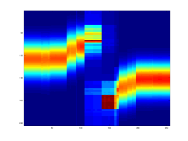
(a) $10^{3}$ observations

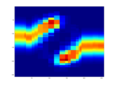
(b) $10^{4}$ observations

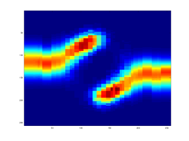
(c) $10^{5}$ observations

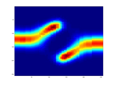
(d) $10^{6}$ observations

Figure 1: Conditional density estimation illustration on a Gaussian ring distribution. It can be seen that the estimator settles on a Gaussian density near the edges, where the distribution is approximately normal, while uses a pseudo-tree distribution near the ring. The structure is refined with subsequent observations.

Figure 1 demonstrates the context model estimator on a ring Gaussian distribution from which samples were generated as follows. Firstly, the mean of a Gaussian was drawn by sampling an angle $\theta$ from a mixture of univariate Gaussians. The observation was then drawn from a bivariate Gaussian with mean equal to the location on a unit ring determined by the drawn angle. Consequently, near and within the ring, the distribution is highly non-Gaussian, while further away from the ring the distribution approaches normality. This is borne out in the figure, since, while in far-away regions, the distribution is modelled with a smooth Gaussian, close to the ring, even for a limited number of samples, the parts of the model which correspond to non-Gaussian distributions have a higher probability.

5.2 Comparisons

We compared our method with a double-kernel conditional density estimator utilising cross-validation for bandwidth selection. This is effectively a Parzen window estimator combined with a kernel density estimator. Although such methods are generally robust, they suffer from two drawbacks. The first is the computational complexity especially in terms of the bandwidth selection for the two kernels. This is something addressed by Holmes et al. (2008), which uses a double tree structure to accelerate the search. The second and most important drawback is that the bandwidth estimator is invariant. This may potentially create problems, since ideally one would like to vary the kernel in different parts of the space. For our quantitative experiments, we utilised a Gaussian kernel throughout for the kernel estimators.

Name	${\mathcal{X}}$	${\mathcal{Y}}$	training	holdout
Gaussian mixture	${\mathds{R}}$	${\mathds{R}}$	$10^{6}$	$10^{6}$
Uniform mixture	${\mathds{R}}$	${\mathds{R}}$	$10^{6}$	$10^{6}$
Geyser	${\mathds{R}}$	${\mathds{R}}$	$200$	$72$
Robot	${\mathds{R}}^{16}$	${\mathds{R}}^{8}$	$2812$	$2644$

Table 1: Summary of datasets

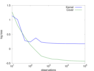
(a) Gaussian mixture

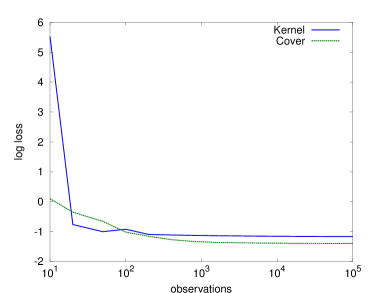
(b) Uniform mixture

(c) Geyser

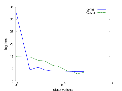
(d) Robot

Figure 2: Conditional density estimation performance on a hold-out set, for four different datasets as the number of observations $t$ increases. The performance is in terms of the relative log loss $L_{t}$ or average negative log-likelihood of the hold-out set. In most cases, the context cover double pseudo-tree significantly outperforms a bandwidth-tuned kernel estimator.

The experimens were performed on a number of datasets, summarised in Table 1. The first two are large, synthetic datasets. The Gaussian mixture dataset is a mixture of three Gaussian distributions on ${\mathds{R}}^{2}$, where the first dimension is used as the conditioning variable. Similarly the Uniform mixture dataset is a mixture of three uniform distributions. We also have results from two real datasets. The first, Geyser, is the well-known dataset of eruption times and durations for the “old faithful” geyser. The second dataset, Robot is a set of proximity sensor readings from a robot performing a navigation task.

For each dataset, we measured the average negative log-likelihood of each method as the amount of training data increased. Each dataset $D$ was split into a training set $D_{T}$ and hold-out set $D_{H}$. For each method, we obtained a sequence of conditional density models $p_{t}$, trained on the subset $D_{t}\subset D_{T}$ of the first $t$ observations in the training set and then calculated the average negative log-likelihood of that model on a hold-out set $D_{h}$:

$$L_{t}\mathrel{\triangleq}-\frac{1}{|D_{h}|}\sum_{(x,y)\in D_{h}}\ln p_{t}(y\mid x).$$ (13)

For the cover method, we employed the same settings as in the previous experiment. For the double-kernel method, for each training subset $D_{t}$, we employed 10-fold cross-validation to select the bandwidths of the two kernels and then used the chosen bandwidths to obtain a model on the full subset $D_{t}$. The criterion for choosing the bandwidth was the likelihood on the left-out folds.

Figure 2 compares the performance of our model with a double-kernel conditional density. One would expect the kernel method to perform best in the Gaussian mixture dataset, while the cover method would be favoured in the uniform mixture. This however, is clearly not the case. Firstly, note that the cover method can optionally use a Normal-Wishart distribution to model the density at any part of the space. Thus, the pure Gaussian kernel has no initial advantage. Secondly, some parts of ${\mathcal{X}}$ have much fewer samples and so would require a much wider kernel for accurate estimation. However, the use of an invariant kernel means that this is not possible. In the uniform mixture dataset, the kernel method is almost as well as the cover method, though it is initially disadvantage due to the bad fit of the Gaussian kernel to the uniform blocks. In the widely-used, although extremely small, Geyser dataset, it can be seen that the kernel method dominates the cover one. However, the difference is quite small and the size of the dataset is such that the performance of the method is mainly dependent upon how well its prior assumptions match the dataset. Finally, in the Robot dataset, which is high-dimensional but has only a moderate number of observations, the methods are more or less evenly matched. The initially bad performance of the kernel method is mainly due to the fact that it is hard to choose a good bandwith from only 100 samples in a high-dimensional space.

Overall, one may observe that the two methods usually perform mostly similarly. However, the cover method appears to be more robust and in some cases its asymptotic performance is significantly better than that of the kernel method.

6 Conclusion

We outlined an efficient, online, closed-form inference procedure for estimation on a sequence of covers. It can be seen as a direct extension of a previous construction (Dimitrakakis, 2010), which was limited to partition trees and an analogous procedure for density estimation on partition trees, given by Hutter (2005).

In principle, the approach is applicable to any problem involving estimation of conditional measures, such as classification and variable order Markov model estimation. As an example, we applied it to conditional density estimation, a fundamental problem in statistics. The result is the first, to our knowledge, closed-form, incremental, polynomial-time, Bayesian conditional density estimation method.

In order to do this, we utilised a double pseudo-tree structure. The first part of the structure was used to estimate the conditional probabilities of context models. The second part of the structure was used to estimate a density for each context. This resulted in a procedure for closed-form, Bayesian, non parametric conditional density estimation. As expected, the performance of this method was in some cases significantly better than that of a kernel based estimator with an invariant kernel.

In future work, we would like to consider other density estimators for the local context models. Since there are virtually no restrictions regarding their type (other than the ability for incremental conditioning), using kernel density estimators on each context instead, could be a route towards obtaining non-invariant kernel density estimation methods. In addition, it would be interesting to consider problems where we have some prior information regarding the smoothness of the underlying conditioning density, perhaps in terms of Lipschitz conditions with respect to the conditioning variable.

The main open problem is how to generate the covers. In this paper, we utilised a kd-tree to do so. However, the generality of the approach is such that many other more interesting alternatives are possible. For example, cover trees (Beygelzimer et al., 2006), which are an extremely efficient nearest-neighbour method, are an ideal alternative. This alternate structure, would allow the application of cover models to an arbitrary metric space. In addition, inference on any lattice structure should remain tractable.

Nevertheless, the problem of finding a suitable sequence of covers remains. This is more pronounced for controlled processes, because one cannot rely on the statistics of the observations to create a useful cover. This problem can be circumvented if a distribution on covers is maintained, which would be more in the spirit of the optional Pólya tree (Wong and Ma, 2010). However, then inference would no longer be closed form.

References

- Beygelzimer et al. (2009) Alina Beygelzimer, John Langford, Yuri Lifshits, Gregory Sorkin, , and Alex Strehl. Conditional probability tree estimation analysis and algorithms. In Uncertainty in Artificial Intelligence (UAI), 2009.
- Beygelzimer et al. (2006) Aline Beygelzimer, Sham Kakade, and John Langford. Cover trees for nearest neighbor. In ICML 2006, 2006.
- DeGroot (1970) Morris H. DeGroot. Optimal Statistical Decisions. John Wiley & Sons, 1970.
- Dimitrakakis (2010) Christos Dimitrakakis. Bayesian variable order Markov models. In Yee Whye Teh and Mike Titterington, editors, Proceedings of the 13th International Conference on Artificial Intelligence and Statistics (AISTATS), volume 9 of JMLR : W&CP, pages 161–168, Chia Laguna Resort, Sardinia, Italy, 2010.
- Holmes et al. (2008) Michael Holmes, Alex Gray, and Charles L. Isbell. Ultrafast Monte Carlo for Kernel Estimators and Generalized Statistical Summations. In Advances in Neural Information Processing Systems (NIPS) 20, 2008.
- Hutter (2005) Marcus Hutter. Fast non-parametric Bayesian inference on infinite trees. In AISTATS 2005, 2005.
- Scott Davies (2002) Andrew Moore Scott Davies. Interpolating conditional density trees. In Conference on Uncertainty in Artificial Intelligence, July 2002.
- Willems et al. (1995) F.M.J. Willems, Y.M. Shtarkov, and T.J. Tjalkens. The context tree weighting method: basic properties. IEEE Transactions on Information Theory, 41(3):653–664, 1995.
- Wong and Ma (2010) W.H. Wong and L. Ma. Optional Pólya tree and Bayesian inference. The Annals of Statistics, 38(3):1433–1459, 2010.