Neutralino versus axion/axino cold dark matter
in the 19 parameter SUGRA model

Abstract:

We calculate the relic abundance of thermally produced neutralino cold dark matter in the general 19 parameter supergravity (SUGRA-19) model. A scan over GUT scale parameters reveals that models with a bino-like neutralino typically give rise to a dark matter density $\Omega_{\tilde{\chi}^{0}_{1}}h^{2}\sim 1-1000$, i.e. between 1 and 4 orders of magnitude higher than the measured value. Models with higgsino or wino cold dark matter can yield the correct relic density, but mainly for neutralino masses around 700-1300 GeV. Models with mixed bino-wino or bino-higgsino CDM, or models with dominant co-annihilation or $A$-resonance annihilation can yield the correct abundance, but such cases are extremely hard to generate using a general scan over GUT scale parameters; this is indicative of high fine-tuning of the relic abundance in these cases. Requiring that $m_{\tilde{\chi}^{0}_{1}}\stackrel{{\scriptstyle<}}{{\sim}}500$ GeV (as a rough naturalness requirement) gives rise to a minimal probably dip in parameter space at the measured CDM abundance. For comparison, we also scan over mSUGRA space with four free parameters. Finally, we investigate the Peccei-Quinn augmented MSSM with mixed axion/axino cold dark matter. In this case, the relic abundance agrees more naturally with the measured value. In light of our cumulative results, we conclude that future axion searches should probe much more broadly in axion mass, and deeper into the axion coupling.

1 Introduction

The cosmic abundance of cold dark matter (CDM) has been recently extracted at high precision by the WMAP collaboration[1]. An analysis of WMAP seven year data implies

$$\Omega_{CDM}h^{2}=0.1123\pm 0.0035\ \ \ (68\%\ CL),$$ (1)

where $\Omega=\rho/\rho_{c}$ is the dark matter density relative to the closure density, and $h$ is the scaled Hubble constant. Since no particle contained within the Standard model of particle physics has exactly the right properties to constitute CDM, new matter states from physics beyond the SM are required for explanation[2].

The most popular explanation of CDM comes from models including weak scale supersymmetry (SUSY)[5]. SUSY models are invoked to cure the hierarchy problem contained within the SM. SUSY models also receive some indirect support from experiment[3] in that the gauge couplings, measured at the scale $Q=M_{Z}$, meet nearly at a point when run to $M_{GUT}$ via the renormalization group equations (RGEs) of the Minimal Supersymmetric Standard Model, or MSSM[4]. Within $R$-parity conserving SUSY theories, there are several dark matter candidates, including the lightest neutralino $\tilde{\chi}^{0}_{1}$, the gravitino $\tilde{G}$ and the axion/axino admixture $a\tilde{a}$ from the Peccei-Quinn[6, 7] augmented MSSM (or PQMSSM).[8]

Most analyses focus upon the lightest neutralino $\tilde{\chi}^{0}_{1}$ as a CDM candidate, since it can be classified as a weakly interacting massive particle, or WIMP. WIMP particles such as $\tilde{\chi}^{0}_{1}$ are especially compelling due to the so-called “WIMP miracle”. It is assumed the DM particle is present in thermal equilibrium at some early time in the universe’s history, and then the relic abundance can be found by solving the Boltzmann equation for its number density. Particles with weak scale mass, which interact with weak scale strength, should give a relic abundance roughly in the vicinity of what is measured.

However, detailed calculations of the neutralino relic abundance in models such as mSUGRA[9] (or CMSSM) find that throughout parameter space, the neutralino abundance is usually much higher than the measured value, and typically by 1-2 orders of magnitude[10]. Only in very narrow regions of parameter space is the measured CDM abundance found: the stau co-annihilation region[12], the hyperbolic branch/ focus point region with mixed higgsino DM[13], the $A$-resonance region at large $\tan\beta$[14], and perhaps at the light Higgs resonance[15].

That the mSUGRA parameter regions where the predicted abundance agrees with measurement are quite narrow is indicative of a needed fine-tuning of fundamental model parameters to achieve the required value. The fine-tuning is a measure of the slope of the surface of $\Omega_{\tilde{\chi}^{0}_{1}}h^{2}$ as a function of model parameters $a_{i}$.

Quantitatively, the fine-tuning with respect to variation in the parameter $a_{i}$ is defined as

$$\Delta_{a_{i}}\equiv\frac{\partial\log\Omega_{DM}h^{2}}{\partial\log a_{i}}.$$ (2)

The overall fine-tuning can be obtained by combining the $\Delta_{a_{i}}$ in quadrature. The degree of fine-tuning of the relic abundance in mSUGRA has been calculated in Ref’s [16] and [17]. Both groups find that the regions of agreement between theory and experiment are highly fine-tuned. Ref. [17] claims also that the very large $\tan\beta$ ($\stackrel{{\scriptstyle>}}{{\sim}}50$) region is not very fine-tuned, since the pseudoscalar Higgs width $\Gamma_{A}$ becomes very large (owing to the large $b$-quark Yukawa coupling), and efficient neutralino annihilation can occur all over the $m_{0}\ vs.\ m_{1/2}$ plane.

In Ref. [18], we proposed mixed axion/axino cold dark matter in the Peccei-Quinn augmented mSUGRA model. By requiring a re-heat temperature in the $10^{6}-10^{8}$ GeV range, a MeV-scale axino mass and a large value of $f_{a}\stackrel{{\scriptstyle>}}{{\sim}}10^{11}$ GeV is favored. As opposed to the high fine-tuning which is present in mSUGRA for neutralino CDM, if instead mixed axion/axino CDM is invoked, with a $\sim$ MeV scale axino[19], then the fine-tuning needed to achieve a theory-experiment match is relatively low. The lowest fine-tuning is observed for the case where there is a nearly equal mix of axion and thermally produced axino DM[17].

A major criticism of the result found in Ref. [17] is that the fine-tuning analysis of neutralino CDM is restricted to the mSUGRA model. It might be possible that if one opens up the parameter space to include models with non-universality, then many more possibilities may arise to gain a theory-experiment match in the dark matter relic density.

In this paper, we calculate the relic abundance of neutralino CDM in a 19 parameter version of the MSSM: the SUGRA-19 model. Another recent calculation of the neutralino CDM abundance in a 19 parameter MSSM has been performed by Berger et al.[20]. In that analysis, the so-called pMSSM model is examined, which is a version of the MSSM with minimal $CP$ and flavor violating terms. The 19 soft SUSY breaking and other parameters are input at the weak scale, and it is required that $\Omega_{\tilde{\chi}^{0}_{1}}h^{2}\leq 0.11$. In the analysis presented here, we will also adopt a 19 parameter MSSM, but will insist on adopting soft SUSY breaking parameters at the GUT scale. The reason is that the unification of gauge couplings provides circumstantial evidence that the MSSM, or MSSM plus gauge singlets (or additional $SU(5)$ multiplets) is the correct effective field theory between $M_{weak}$ and $M_{GUT}$. The pattern of soft term running as provided by the MSSM RGEs gives us some guidance as to how likely are various sets of weak scale parameters. For instance, by sampling over weak scale parameters including the superpotential $\mu$ term, one easily generates low $\mu$ solutions which lead to higgsino-like neutralinos. However, sampling over GUT scale parameters, it is not easy to generate low $\mu$ solutions with higgsino-like dark matter. The reason is that (at tree level) $\mu^{2}(m_{weak})\simeq-m_{H_{u}}^{2}(M_{weak})$, and it is rare that $m_{H_{u}}^{2}$ runs to just barely negative values, which would lead to a small $\mu$ parameter. In addition, in distinction with Ref. [20], we will not restrict ourselves to requiring $\Omega_{\tilde{\chi}^{0}_{1}}h^{2}<0.11$, but will instead allow all values of thermal neutralino abundance.

In Sec. 2, we provide an overview of our scanning methodology and parameter space values, and our calculation of the neutralino relic abundance. In Sec. 3, we present results of the neutralino relic density from a scan over the SUGRA-19 model. We find that solutions with bino-like neutralinos give a large overabundance of CDM. Models with higgsino-like or wino-like neutralinos tend to give too little CDM, unless $m_{\tilde{\chi}^{0}_{1}}\sim 1$ TeV, with observable sparticles likely beyond LHC reach. The value $\Omega_{\tilde{\chi}^{0}_{1}}h^{2}\sim 0.11$ lies at the minimum probability between these two extremes. Since our scan depends on the bias as to how we sample the GUT scale parameters, we present results for both a linear as well as a log scan; the latter scan accentuates small soft SUSY breaking parameter values. In Sec. 3.3, we present for comparison a similar analysis done for the mSUGRA model. In Sec. 4, we work instead within the Peccei-Quinn augmented MSSM, or PQMSSM, which leads to mixed axion/axino CDM if the axino is assumed to be the lightest SUSY particle (LSP). The PQMSSM requires four additional parameters: the PQ breaking scale $f_{a}$ and initial mis-alignment angle $\theta_{i}$, the axino mass $m_{\tilde{a}}$, and the re-heat temperature of the universe $T_{R}$. In this case, the PQMSSM with 23 free parameters can more easily yield the measured relic abundance. We evaluate the favored range of the additional PQMSSM parameters. Our conclusions are presented in Sec. 5.

2 Relic density in the SUGRA-19 model

For our calculations, we adopt the Isajet 7.80[24, 25] SUSY spectrum generator Isasugra. Isasugra begins the calculation of the sparticle mass spectrum with input $\overline{DR}$ gauge couplings and $f_{b}$, $f_{\tau}$ Yukawa couplings at the scale $Q=M_{Z}$ ($f_{t}$ running begins at $Q=m_{t}$) and evolves the 6 couplings up in energy to scale $Q=M_{GUT}$ (defined as the value $Q$ where $g_{1}=g_{2}$) using two-loop RGEs. At $Q=M_{GUT}$, the SSB boundary conditions are input, and the set of 26 coupled two-loop MSSM RGEs[26] are evolved back down in scale to $Q=M_{Z}$. Full two-loop MSSM RGEs are used for soft term evolution, while the gauge and Yukawa coupling evolution includes threshold effects in the one-loop beta-functions, so the gauge and Yukawa couplings transition smooothly from the MSSM to SM effective theories as different mass thresholds are passed. In Isajet 7.80, the values of SSB terms which mix are frozen out at the scale $Q\equiv M_{SUSY}=\sqrt{m_{\tilde{t}_{L}}m_{\tilde{t}_{R}}}$, while non-mixing SSB terms are frozen out at their own mass scale[25]. The scalar potential is minimized using the RG-improved one-loop MSSM effective potential evaluated at an optimized scale $Q=M_{SUSY}$ which accounts for leading two-loop effects[27]. Once the tree-level sparticle mass spectrum is computed, full one-loop radiative corrections are caculated for all sparticle and higgs boson masses, including complete one-loop weak scale threshold corrections for the top, bottom and tau masses at scale $Q=M_{SUSY}$. These fermion self-energy terms are critical to evaluating whether or not Yukawa couplings do indeed unify. Since the GUT scale Yukawa couplings are modified by the threshold corrections, the Isajet RGE solution must be imposed iteratively with successive up-down running until a convergent sparticle mass solution is found. For most of parameter space, there is excellent agreement between Isajet and the SoftSUSY, SuSpect and Spheno codes, although at the edges of parameter space agreement between the four codes typically diminishes[28]. We adopt the Isasugra non-universal SUGRA parameter space.

We will implement at first a linear scan over the following parameters.

• Gaugino masses: $M_{1},\ M_{2},\ M_{3}:0-3.5$ TeV

• First/second generation scalar masses: $m_{Q_{1}}$, $m_{U_{1}}$, $m_{D_{1}}$, $m_{L_{1}}$, $m_{E_{1}}$: $0-3.5$ TeV,

• Third generation scalar masses: $m_{Q_{3}}$, $m_{U_{3}}$, $m_{D_{3}}$, $m_{L_{3}}$, $m_{E_{3}}$: $0-3.5$ TeV,

• Higgs soft masses: $m_{H_{u}},\ m_{H_{d}}:\ 0-3.5$ TeV,

• trilinear soft terms: $A_{t},\ A_{b},\ A_{\tau}$:$-3.5\ {\rm TeV}\ \rightarrow 3.5$ TeV,

• ratio of weak scale Higgs vevs $\tan\beta:\ 2-60$.

We adopt a common mass for first and second generation scalars so as to avoid SUSY FCNC processes.

To gain an acceptable sparticle mass solution, we will require:

1. the lightest SUSY particle (LSP) is the neutralino $\tilde{\chi}^{0}_{1}$,

2. the lightest chargino, if non-wino-like, obeys the LEP2 limit $m_{\tilde{\chi}_{1}}>103.5$ GeV,

3. the lightest chargino, if wino-like, obeys the LEP2 limit $m_{\tilde{\chi}_{1}}>91.9$ GeV,

4. the light Higgs mass obeys the LEP2 limit $m_{h}>111$ GeV (where we allow a roughly 3 GeV uncertainty in the theory calculation as applied to the actual limit where $m_{h}>114.4$ GeV.

For each acceptable solution, we calculate the neutralino relic density $\Omega_{\tilde{\chi}^{0}_{1}}h^{2}$ using the IsaReD[29] program. IsaReD calculates all relevant neutralino annihilation and co-annihilation reactions, as obtained using CalcHEP, and then calculates the relativistic thermally-averaged (co)-annihilation cross sections times relative velocity. Once the freeze-out temperature is determined, then the relic density at the present time is found by integrating the Boltzmann equation as formulated for a FRW universe.

Since we assume the neutralino to be in thermal equilibrium, our relic density results do not explicitly depend on the value of the re-heat temperature of the Universe $T_{R}$ after inflation. However, we must assume $T_{R}>T_{fo}\sim m_{\tilde{\chi}^{0}_{1}}/20$ so that $T_{R}$ is above the neutralino freeze-out temperature. Further, if $T_{R}\stackrel{{\scriptstyle>}}{{\sim}}10^{10}$ GeV, then thermal production of gravitinos in the early Universe, followed by decays to the LSP, will overproduce neutralino dark matter. Hence, for our neutralino CDM relic density calculations, we must assume here that

• $m_{\tilde{\chi}^{0}_{1}}/20\stackrel{{\scriptstyle<}}{{\sim}}T_{R}\stackrel{{\scriptstyle<}}{{\sim}}10^{10}$ GeV.

3 Results for neutralino cold dark matter

3.1 Linear scan over SUGRA-19 parameters

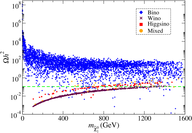
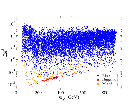
Our first results from a linear scan over the above SUGRA-19 parameter space is shown in Fig. 1, in the $\Omega_{\tilde{\chi}^{0}_{1}}h^{2}\ vs.\ m_{\tilde{\chi}^{0}_{1}}$ plane. The various solutions are color coded according to the gaugino/higgsino content of the neutralino. In the notation of Ref. [5], if the bino-component $|v_{4}^{(1)}|>0.9$, then the neutralino is labeled as bino-like (blue diamonds); if the wino-component $|v_{3}^{(1)}|>0.9$, then it is labeled wino-like (purple $\times$); if the higgsino components $\sqrt{v_{1}^{(1)2}+v_{2}^{(1)2}}>0.9$, then it is labeled as higgsino-like (red squares). If the neutralino falls into none of these categories, then it is labeled as “mixed” DM: (orange circles).

We see from Fig. 1 that the bino-like neutralinos tend to populate the region with $\Omega_{\tilde{\chi}^{0}_{1}}h^{2}\gg 0.1$, i.e. usually about 2-3 orders of magnitude too high. For low values of $m_{\tilde{\chi}^{0}_{1}}$, the abundance tends to be more like 3-5 orders of magnitude too high. A few bino-like points do tend to make it into the $\Omega_{\tilde{\chi}^{0}_{1}}h^{2}\sim 0.1$ region; these solutions tend to come form various co-annihilation or resonance annihilation processes. To obtain the required relic abundance via co-annihilation, the LSP-NLSP mass gap must be tuned to just the right value. To obtain the required relic abundance via resonance annihilation, the LSP mass must be adjusted to be close to half the mass of the resonance. These co-annihilation and resonance annihilation points are quite hard, but not impossible, to generate using our random scan over GUT scale parameters.

The higgsino-like and wino-like CDM bands also show up as distinct lines, typically with $\Omega_{\tilde{\chi}^{0}_{1}}h^{2}$ too low by 1-2 orders of magnitude unless $m_{\tilde{\chi}^{0}_{1}}\stackrel{{\scriptstyle>}}{{\sim}}800-1200$ GeV. The wino-like band is relatively well-populated, as this just requires $M_{2}$ to be the lightest of the gaugino masses at the weak scale. The higgsino-like band is relatively less populated, showing that higgsino-like CDM is rather fine-tuned if one starts with GUT scale parameters, as mentioned in Sec. 1. The points with the lowest population are those with mixed bino-higgsino-wino CDM. These “well-tempered neutralino[31]” points most naturally tend to populate the $\Omega_{\tilde{\chi}^{0}_{1}}h^{2}\sim 0.1$ line, but they do require a fine-tuning to avoid a bino, wino or higgsino dominance. Especially at low $m_{\tilde{\chi}^{0}_{1}}$, relatively few solutions are found with $\Omega_{\tilde{\chi}^{0}_{1}}h^{2}\sim 0.1$.

Figure 1: Thermal abundance of neutralino cold dark matter from a linear scan over the SUGRA-19 parameter space. We plot versus the neutralino mass. Models with mainly bino, wino, higgsino or a mixture are indicated by the various color and symbol choices. There are 5252 points in the figure.

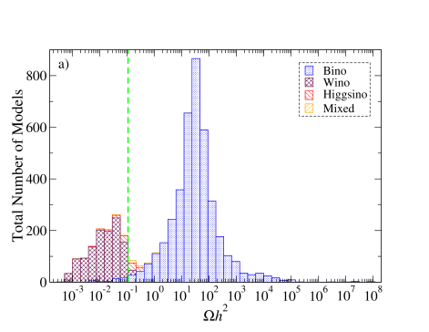
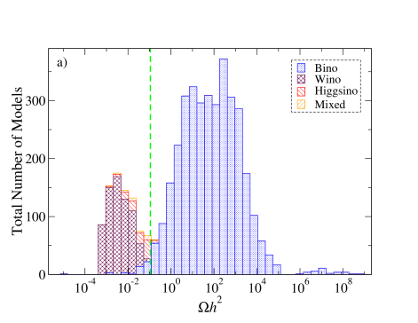
To apprehend more clearly the dark matter probability distribution after our linear scan of SUGRA-19 parameter space, we project the model points listed in Fig. 1 as a histogram onto the $\Omega_{\tilde{\chi}^{0}_{1}}h^{2}$ axis in Fig. 2a). Here we see the most probable value of $\Omega_{bino}h^{2}$ is $\sim 10-100$ for bino-like dark matter (blue histogram), while the most probable value for wino-like dark matter is $\Omega_{wino}h^{2}\sim 0.005-0.05$. The dip between these two cases is partially filled in by cases of bino, higgsino or wino, or a mixture, with the minimum probability lying around $\Omega_{\tilde{\chi}^{0}_{1}}h^{2}\sim 0.2-0.4$, i.e. just above the measured value.

Figure 2: Projection of the number of models generated by a linear scan over SUGRA-19 parameters, versus neutralino relic density $\Omega_{\tilde{\chi}^{0}_{1}}h^{2}$. Models with mainly bino, wino, higgsino or a mixture are indicated by the various color and symbol choices. In frame b)., we require only models with $m_{\tilde{\chi}^{0}_{1}}<500$ GeV to avoid too large of fine-tuning in the SUSY parameters.

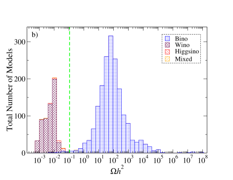
A large number of the wino and higgsino dark matter solutions with $\Omega_{\tilde{\chi}^{0}_{1}}h^{2}\sim 0.1$ come from models with very heavy neutralinos: $m_{\tilde{\chi}^{0}_{1}}\stackrel{{\scriptstyle>}}{{\sim}}800$ GeV. If the $\tilde{\chi}^{0}_{1}$ is the LSP, as assumed here, then all other sparticles are heavier– and usually much heavier– than this value, and will likely lead to solutions with high electroweak fine-tuning[32]. In Fig. 2b)., we plot the number of model solutions from the SUGRA-19 scan versus $m_{\tilde{\chi}^{0}_{1}}$, where in addition we require (somewhat arbitrarily) that $m_{\tilde{\chi}^{0}_{1}}<500$ GeV, so the solutions are not too fine-tuned with regard to electroweak symmetry breaking. In this case, the higgsino and wino LSP models which naturally give $\Omega_{\tilde{\chi}^{0}_{1}}h^{2}\sim 0.1$ are all excluded. The maxima of bino-like solutions has moved up slightly to $\Omega_{\rm bino}h^{2}\sim 50-100$, while wino-like solutions peak at $\Omega_{\rm wino}h^{2}\sim 0.01$. The minimum of the probability distribution lies very close to the measured value $\Omega_{\rm CDM}h^{2}\sim 0.1$. With sparticle masses generally at the TeV or below scale, the measured relic density lies at the least likely value as predicted by the SUGRA-19 model. In this case, it would be extremely fortuitous if the lightest neutralino of SUGRA theories was in fact the dark matter particle.

3.2 Log scan over SUGRA-19 parameters

We have interpreted our linear scan over SUGRA-19 parameter space in terms of a probability distribution as to likely values of $\Omega_{\tilde{\chi}^{0}_{1}}h^{2}$ which would be obtained in supersymmetric models. These results do depend on how we sample our GUT-scale parameter space. While it is impossible to know what the correct measure is for GUT-scale SUSY parameters, at least we can compare our linear scan against results using a different sampling measure for our parameter space.

In this section, we will instead adopt a logarithmic scan over GUT scale parameters, which favors lower energy soft SUSY breaking parameters over high energy ones. Specifically, for a dimensionful parameter $a$ ranging up to $a_{max}$, and a random number $x$ which is sampled uniformly between 0 and 1, we will generate values of $a$ according to $a=\exp\left(x\log(a_{max})\right)$.

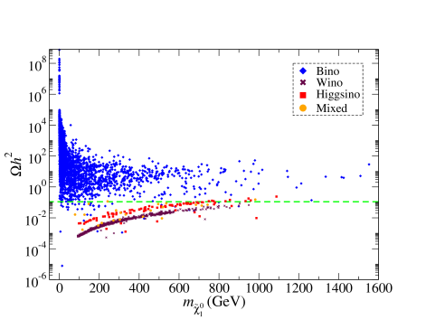
Applying the log sampling to all dimensionful parameters listed in Sec. 2 (but with a linear scan over $\tan\beta$), and with the same parameter maxima, we re-plot our results in Fig. 3. Here, we see that models with lower values of $m_{\tilde{\chi}^{0}_{1}}$ are sampled much more prominently than high values of $m_{\tilde{\chi}^{0}_{1}}$. In the figure, we see that while bino-like models still predict a rather high relic density, now there are some bino-like LSP points with relatively small values of $m_{\tilde{\chi}^{0}_{1}}$ and $\Omega_{\tilde{\chi}^{0}_{1}}h^{2}\sim 0.1$. Meanwhile, the higgsino-like and wino-like bands still persist at the same location as in Fig. 1, albeit with a greater population of points at low $m_{\tilde{\chi}^{0}_{1}}$. We also obtain some mixed dark matter solutions at low $m_{\tilde{\chi}^{0}_{1}}$.

Figure 3: Thermal abundance of neutralino cold dark matter from a log scan over SUGRA-19 model parameter space. We plot versus the neutralino mass. Models with mainly bino, wino, higgsino or a mixture are indicated by the various color and symbol choices. There are 4276 points in the figure.

To compare against the previous distribution in models (Fig. 2), we again project the models as a histogram on the $\Omega_{\tilde{\chi}^{0}_{1}}h^{2}$ axis in Fig. 4a). While the minimum in the probability distribution still lies nearly at the measured CDM abundance, the minimum has filled in somewhat, especially with a mixture of bino-like and higgsino-like solutions.

Figure 4: Projection of the number of models generated by a log scan over SUGRA-19 parameter space, versus neutralino relic density $\Omega_{\tilde{\chi}^{0}_{1}}h^{2}$. In frame b)., we require only models with $m_{\tilde{\chi}^{0}_{1}}<500$ GeV to avoid too large of fine-tuning in the SUSY parameters. Models with mainly bino, wino, higgsino or a mixture are indicated by the various color and symbol choices.

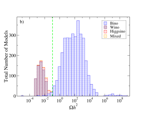
For comparison with Fig. 2b)., we apply the requirement of $m_{\tilde{\chi}^{0}_{1}}<500$ GeV and gain the results shown in Fig. 4b). In this case, the minimum probability has migrated to slightly lower values, as the higgsino-like and wino-like solutions with $\Omega_{\tilde{\chi}^{0}_{1}}h^{2}\sim 0.1$ require $m_{\tilde{\chi}^{0}_{1}}\stackrel{{\scriptstyle>}}{{\sim}}800$ GeV, and have been rejected. We still have a few bino-like models persisting with $\Omega_{\tilde{\chi}^{0}_{1}}h^{2}\sim 0.1$, although the probability is again quite small (but not as small as in the linear sampling case).

3.3 Comparison of SUGRA-19 results to the mSUGRA model

In this section, for comparison purposes, we present similar results if we restrict our scan to the mSUGRA model with the well-known parameter space

$$m_{0},\ m_{1/2},\ A_{0},\ \tan\beta,\ sign(\mu),$$ (3)

with $m_{t}=173.1$ GeV as before. We sample $m_{0}:0-6$ TeV, $m_{1/2}:0-2$ TeV, $A_{0}:-3.5\rightarrow 3.5$ TeV and $\tan\beta:2\rightarrow 60$. This expands upon the treatment presented in Ref. [11], since it provides a general scan over mSUGRA parameters. We only present results of the linear scan for this case. The results of our scan are shown in Fig. 5, in the $\Omega_{\tilde{\chi}^{0}_{1}}h^{2}\ vs.\ m_{\tilde{\chi}^{0}_{1}}$ plane. We again see that bino-like neutralino solutions populate the high $\Omega_{\tilde{\chi}^{0}_{1}}h^{2}$ region, while higgsino-like and mixed bino-higgsino dark matter solutions (arising from the focus point region) populate the range from $\Omega_{\tilde{\chi}^{0}_{1}}h^{2}\sim 0.01-0.3$. The nearly pure higgsino solutions are almost always lower than the measured DM abundance. The wino-like CDM solutions have vanished, since in this case, with gaugino mass unification at $M_{GUT}$, we always get gaugino masses $M_{1}\ll M_{2}$ at the weak scale.

Figure 5: Thermal abundance of neutralino cold dark matter from a linear scan over the mSUGRA model parameter space. We plot versus the neutralino mass. Models with mainly bino, wino, higgsino or a mixture are indicated by the various color and symbol choices. There are 10,025 points in the figure.

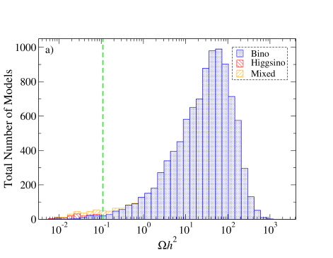
In Fig. 6a)., we project the solutions onto the $\Omega_{\tilde{\chi}^{0}_{1}}h^{2}$ axis. The prevalence of bino-like DM solutions is clear, with a maximum around $\Omega_{\tilde{\chi}^{0}_{1}}h^{2}\sim 30-50$. A tail drops off gradually at low values of $\Omega_{\tilde{\chi}^{0}_{1}}h^{2}$, although the tail flattens for a while when it is augmented by the appearance of higgsino-like and mixed bino-higgsino DM solutions near the measured value of $\Omega_{\tilde{\chi}^{0}_{1}}h^{2}\sim 0.1$.

Figure 6: Projection of the number of models generated by a linear scan over mSUGRA parameters, versus neutralino relic density $\Omega_{\tilde{\chi}^{0}_{1}}h^{2}$. In frame b)., we require only models with $m_{\tilde{\chi}^{0}_{1}}<500$ GeV to avoid too large of fine-tuning in the SUSY parameters. Models with mainly bino, wino, higgsino or a mixture are indicated by the various color and symbol choices.

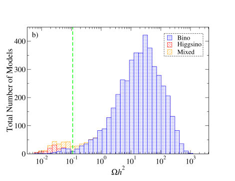
If we apply the rough electroweak naturalness requirement that $m_{\tilde{\chi}^{0}_{1}}<500$ GeV, we arrive at the results in Fig. 6b). In this case, many of the higgsino-like solutions with $\Omega_{\tilde{\chi}^{0}_{1}}h^{2}\sim 0.1$ are now excluded, and the measured relic density lies again at a slight dip between the large bino-like maximum and the softer mixed bino-higgsino maximum around $\Omega_{\tilde{\chi}^{0}_{1}}h^{2}\sim 0.03$. By comparing Fig. 6b). for the mSUGRA model against Fig. 2b). for SUGRA-19, we conclude that it is actually easier to generate the measured abundance of CDM in mSUGRA than in the more expansive SUGRA-19 parameter space.

4 Scan over PQMSSM with mixed axion/axino cold dark matter

In this section, we assume the MSSM augmented by the Peccei-Quinn mechanism (PQMSSM) is the correct effective field theory below the scale $T_{R}$. Thus, the MSSM is supplemented by an axion supermultiplet containing the spin-zero and $R$-parity even axion $a$ and saxion $s$ fields, and the $R$-odd spin-$1\over 2$ axino field $\tilde{a}$. We assume the axino is the LSP, and one of the constituents of dark matter. We do not assume a specific axion model, e.g. KSVZ[33] or DFSZ[34], nor do we assume a specific SUSY breaking mechanism to give the axino mass. We parametrize the low energy axion/axino physics by adopting as free parameters the PQ breaking scale $f_{a}/N$ (where $N$ is the model-dependent color anomaly), the axino mass $m_{\tilde{a}}$ (for which $m_{\tilde{a}}<m_{\tilde{\chi}^{0}_{1}}$) the re-heat temperature $T_{R}$ (which is related to unknown inflaton parameters) and the axion field initial mis-alignment angle $\theta_{i}$.

We will assume a re-heat temperature $T_{R}$ bounded by $min[10^{10}\ {\rm GeV},T_{dcp}]$, where $T_{dcp}\sim 10^{11}\left(\frac{f_{a}/N}{10^{12}\ {\rm GeV}}\right)^{2}$ GeV, so as to be consistent with results from Sec. 3, which avoided overclosure limits from excessive gravitino production in the early universe[35]. This limit also avoids the RTW bound[36] $T_{R}\stackrel{{\scriptstyle>}}{{\sim}}T_{\rm dcp}$ for which axinos would be in thermal equilibrium in the early universe. We will also assume $m_{\tilde{a}}\stackrel{{\scriptstyle>}}{{\sim}}100$ keV; for lighter axino masses, the thermally produced axinos (see below) would likely constitute warm, rather than cold, dark matter[37]. Thus, we supplement the SUGRA-19 model by an axion/axino supermultiplet along with the additional parameters

• $f_{a}/N:\ 10^{9}\rightarrow 10^{16}$ GeV,

• $m_{\tilde{a}}:\ 100\ {\rm keV}\rightarrow m_{\tilde{\chi}^{0}_{1}}$,

• $T_{R}:max[0.01\ {\rm GeV},m_{\tilde{\chi}^{0}_{1}}/20]\rightarrow min[10^{10}\ {\rm GeV},T_{dcp}]$,

• $\theta_{i}:-\pi\rightarrow\pi$.

The lower bound on $f_{a}/N$ comes from bounds on red giant cooling and supernova 1987a. The upper bound on $f_{a}/N$ we take near the GUT scale. The more common bound $f_{a}/N\stackrel{{\scriptstyle<}}{{\sim}}10^{12}$ GeV comes from assuming $\theta_{i}\sim 1$. The lower bound on $T_{R}$ comes from requiring $T_{R}\stackrel{{\scriptstyle>}}{{\sim}}10$ MeV so that standard BBN can occur[38], and requiring neutralino production at temperatures above neutralino freeze-out.

4.1 Mixed axion/axino relic density

In this section, we briefly review dark matter production in the PQMSSM, with an axino as LSP. Since we assume a value $T_{R}\stackrel{{\scriptstyle<}}{{\sim}}10^{10}$ GeV, then axinos should never be in thermal equilibrium in the early universe[36]. However, thermal production of neutralinos (now assumed to be the NLSP) should proceed as usual, except that now each neutralino will decay via $\tilde{\chi}^{0}_{1}\rightarrow\tilde{a}\gamma$. Since the $\tilde{\chi}^{0}_{1}$ lifetime is of order $0.1$ sec, it is assumed to be BBN-safe. This non-thermal contribution to the axino CDM abundance is given by

$$\Omega_{\tilde{a}}^{NTP}=\frac{m_{\tilde{a}}}{m_{\tilde{\chi}^{0}_{1}}}\Omega_{\tilde{\chi}^{0}_{1}}h^{2}$$ (4)

since the axino number density from this source is the same as the thermally produced neutralino number abundance.

While the axinos are assumed never in thermal equilibrium in the early universe, nevertheless, they can still be produced thermally via radiation off of particles that are in thermal equilibrium, i.e. the quarks, leptons, gluons, SUSY particles etc.. This thermal axino production mechanism has been calculated in Ref’s [40], [41] and [42]. The latter calculation includes some interaction terms neglected in previous calculations; they find

$$\Omega_{\tilde{a}}^{TP}h^{2}\simeq 1.24g_{s}^{4}F(g_{s})\frac{m_{\tilde{a}}}{{\rm GeV}}\frac{T_{R}}{10^{4}\ {\rm GeV}}\left(\frac{10^{11}\ {\rm GeV}}{f_{a}/N}\right)^{2}\ \ \ F(g_{s})\simeq 20g_{s}^{2}\ln\frac{3}{g_{s}}$$ (5)

where $g_{s}$ is the strong coupling evaluated at $Q=T_{R}$ (e.g. $g_{s}(T_{R}=10^{6}\ {\rm GeV})=0.932$, as given by Isajet 2-loop $g_{s}$ evolution in mSUGRA).

Finally, relic axions will be produced via the vacuum mis-alignment mechanism. In this case, we use[43, 44]

$$\Omega_{a}h^{2}={1\over 4}f(\theta_{i})\theta_{i}^{2}\left(\frac{f_{a}/N}{10^{12}\ {\rm GeV}}\right)^{7/6},$$ (6)

where $f(\theta_{i})$ is the anharmonicity factor. We adopt a recent parametrization of $f(\theta_{i})$ from Visinelli and Gondolo[44] given by

$$f(\theta_{i})=\left[\ln\left(\frac{e}{1-\theta_{i}^{2}/\pi^{2}}\right)\right]^{7/6}.$$ (7)

The function $f(\theta_{i})\rightarrow 1$ as $\theta_{i}\rightarrow 0$ and $f(\theta_{i})\rightarrow\infty$ as $\theta_{i}\rightarrow\pm\pi$.

The total dark matter abundance in the PQMSSM with an axino LSP is then given by the sum of the three constituents:

$$\Omega_{a\tilde{a}}h^{2}=\Omega_{\tilde{a}}^{NTP}h^{2}+\Omega_{\tilde{a}}^{TP}h^{2}+\Omega_{a}h^{2}.$$ (8)

4.2 Results of scan over SUGRA-19 with mixed $a\tilde{a}$ CDM

Our first results from the linear scan over SUGRA-19 model parameters augmented by the four PQMSSM parameters are shown in Fig. 7, where we plot models generated in the $\Omega_{a\tilde{a}}h^{2}\ vs.\ f_{a}/N$ plane. Models with dominant axion CDM are in red, while models with dominant axino CDM are in blue. The measured CDM abundance is denoted by the dashed green line. The densely populated diagonal band which increases as $f_{a}/N$ increases is due to mainly axion CDM with $\theta_{i}\sim 1$. The diffuse dotted region at low $f_{a}/N$, which extends up to very large values of $\Omega_{a\tilde{a}}h^{2}\sim 10^{9}$ is due to thermally produced axinos. For thermally produced axinos, the axino-matter coupling is inversley proportional to $f_{a}/N$, and so the coupling is large at low $f_{a}/N$ values, leading to the large thermal abundance. As $f_{a}/N$ increases, the axino-matter coupling is suppressed, while the magnitude of the axion vacuum energy increases, leading to the case of mixed axion/axino CDM which is mainly axions.

Figure 7: SUGRA-19 parameter space points from a linear scan where we assume mixed axion/axino CDM. There are 4217 points in the figure.

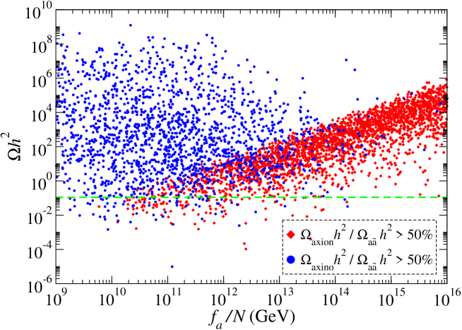
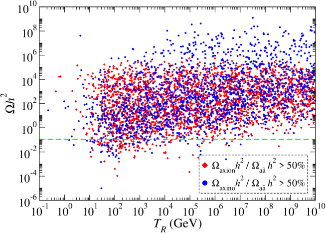
In Fig. 8, we plot models in the $\Omega_{a\tilde{a}}h^{2}\ vs.\ T_{R}$ plane. In this case, we see the models are spread over a wide range of $T_{R}$ values. Large values of $T_{R}$ give rise to a large rate for thermally produced axinos, and so $\Omega_{a\tilde{a}}$ increases somewhat with increasing $T_{R}$. In fact, it becomes difficult, but not impossible, to gain a value of $\Omega_{a\tilde{a}}h^{2}\sim 0.1$ while maintaining $T_{R}\stackrel{{\scriptstyle>}}{{\sim}}10^{6}$ GeV, as needed for baryogenesis processes such as non-thermal leptogenesis[45]. Since the axion abundance doesn’t depend on $T_{R}$, the low $T_{R}$ points are dominanted by mainly axion CDM models.

Figure 8: Scan over the PQMSSM parameter space plotted in the $\Omega_{a\tilde{a}}h^{2}\ vs.\ T_{R}$ plane

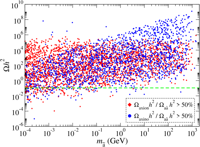
In Fig. 9, we plot models in the $\Omega_{a\tilde{a}}h^{2}\ vs.\ m_{\tilde{a}}$ plane. Here, we see the models are spread rather uniformly over many decades of $m_{\tilde{a}}$, although the tendency is for $\Omega_{a\tilde{a}}h^{2}$ to increase as $m_{\tilde{a}}$ increases. This is partly due to the fact that each relic axino is more massive.

Figure 9: SUGRA-19 parameter space points from a linear scan where we assume mixed axion/axino CDM.

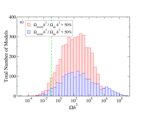
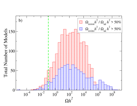
To compare against results from our thermal neutralino calculations of Sec. 3, we project all the models onto the $\Omega_{a\tilde{a}}h^{2}$ axis, and present our results as a histogram in the number of models generated. We see from frame a). of Fig. 10 that the models are spread over many decades of $\Omega_{a\tilde{a}}h^{2}$. The measured abundance– denoted by the green dashed line– lies on the rising shoulder of the distribution, which in fact peaks around $\Omega_{a\tilde{a}}h^{2}\sim 10^{2}$. If we require in addition $m_{\tilde{\chi}^{0}_{1}}<500$ GeV as in Fig. 2b). as a rough EW fine-tuning requirement, then we obtain the results of frame b). Qualitatively, the two plots are similar, and the measured abundance still lies on the increasing shoulder of the distribution, which again peaks around $\Omega_{a\tilde{a}}h^{2}\sim 100$.

Figure 10: Number of models versus $\Omega_{a\tilde{a}}h^{2}$ in the scan over the PQMSSM parameter space. Frame a). contains all models. Frame b). requires $m_{\tilde{\chi}^{0}_{1}}<500$ GeV, as a rough constraint due to electroweak fine-tuning.

4.3 PQMSSM parameters which are preferred by the measured CDM abundance

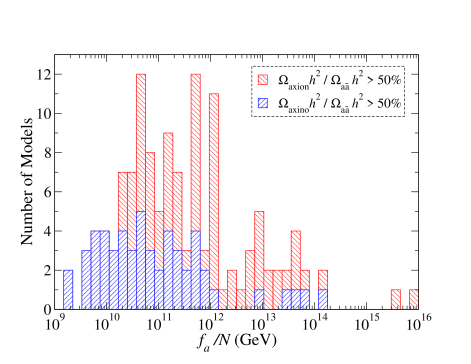
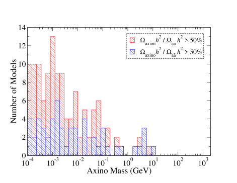
As a final exercise, it may be instructive to see which values of PQMSSM parameters are preferred by the measured abundance of CDM in the universe. To this end, we will require $\Omega_{a\tilde{a}}h^{2}$ to lie between 0.05 and 0.2: i.e. within a factor of two of the measured abundance. Then we can project our random scans on the parameter axis.

In Fig. 11, we project the PQMSSM models onto the $f_{a}/N$ plane. In this case, we see that the measured CDM abundance prefers a value of $f_{a}/N\sim(1-2)\times 10^{11}$ GeV, with broad tails extending to higher and lower values. This value of $f_{a}/N$ corresponds to that which is needed for PQMSSM models with mainly axion CDM and initial mis-alignment angle of order 1-2.

Figure 11: SUGRA-19 parameter space points from a linear scan where we assume mixed axion/axino CDM.

In Fig. 12, we show PQMSSM models with the measured abundance versus axino mass $m_{\tilde{a}}$. Here, the value of $m_{\tilde{a}}$ is spread over many decades, with some favoritism for small values of $m_{\tilde{a}}\sim$ MeV range. These again correspond to the models with mainly axion CDM.

Figure 12: SUGRA-19 parameter space points from a linear scan where we assume mixed axion/axino CDM.

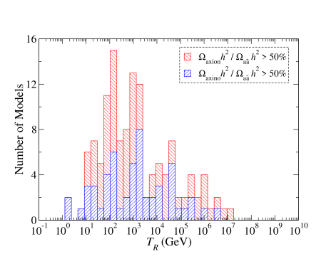
In Fig. 13, we show PQMSSM models with the measured abundance versus re-heat temperature $T_{R}$. The $T_{R}$ values are spread out over many decades. There is some preference for low values of $T_{R}$ in the GeV range, since these models suppress excess thermal axino production while allowing for vacuum mis-alignment production of relic axions, which don’t depend on $T_{R}$. The high $T_{R}$ tail does extend up to values of $T_{R}$ as high as $10^{6}-10^{7}$ GeV, which can allow for baryogenesis via non-thermal leptogenesis.

Figure 13: SUGRA-19 parameter space points from a linear scan where we assume mixed axion/axino CDM.

5 Summary and conclusions

In this paper, we have reported on a calculation of the thermal abundance of relic neutralinos in the SUGRA-19 model with 19 free parameters, where all dimensional parameters are stipulated at the GUT scale, as suggested by gauge coupling unification, and SUSY GUTs[4]. We find in this rather general framework that bino-like neutralinos populate the high $\Omega_{\tilde{\chi}^{0}_{1}}h^{2}\sim 10^{1}-10^{3}$ region, while wino and higgsino-like neutralinos tend to populate the $\Omega_{\tilde{\chi}^{0}_{1}}h^{2}\sim 10^{-3}-10^{-2}$ region. The measured CDM abundance sits at a deep minimum between these two favored values, especially if one requires rather light sparticles with $m_{\tilde{\chi}^{0}_{1}}\stackrel{{\scriptstyle<}}{{\sim}}500$ GeV, as suggested by electroweak fine-tuning arguments. In this region, a “well-tempered neutralino” is needed; however, these WTNs with the correct relic abundance are very difficult to generate using GUT scale SUSY breaking parameters. In this case, we conclude that it would be a near miracle if SUSY neutralinos were to constitute the measured CDM in the universe. This is the opposite conclusion to that suggested by the “WIMP miracle”, where it is asserted that WIMPs have exactly the right properties to constitute thermal relics of the Big Bang. In the case of SUSY WIMPs, this does not appear to be so.

Our results were presented in the context of a linear scan over SUGRA-19 parameters, but remain qualitatively valid in the case of a log scan over parameter space. We also compare our results with those obtained in the minimal SUGRA or CMSSM model, where wino-like $\tilde{\chi}^{0}_{1}$s don’t appear. In the case of mSUGRA, the constrained GUT scale parameter choices actually make neutralino CDM somewhat more likely than in the SUGRA-19 case.

If the strong CP problem is solved by the PQ mechanism in the context of SUSY models, then an attractive alternative for dark matter appears: mixed axion/axino CDM. A scan over SUGRA-19 parameters, augmented by four extra PQMSSM parameters, shows that the mixed axion/axino DM abundance can be generated. While the measured CDM abundance doesn’t lie at the peak of the predicted $a\tilde{a}$ abundance, it also doesn’t lie at a minimum. Therefore, in our viewpoint, the mixed axion/axino particles seem a more plausible candidate for CDM.

In the end, the issue will have to be resolved by experiment. A thorough search for relic axions with $f_{a}/N\sim 10^{9}-10^{16}$ GeV is needed. Currently, only a tiny portion of QCD axion parameter space has been explored[46]. A major consequence of our analysis then is to motivate our experimental colleagues to consider the possibility of new, more encompassing probes of axion dark matter. These should probe much more broadly in axion mass, and much more deeply in axion coupling.