How the diffusivity profile reduces the arbitrariness of protein folding free energies
Abstract
The concept of a protein diffusing in its free energy folding landscape has been fruitful for both theory and experiment. Yet the choice of the reaction coordinate (RC) introduces an undesirable degree of arbitrariness into the problem. We analyze extensive simulation data of an -helix in explicit water solvent as it stochastically folds and unfolds. The free energy profiles for different RCs exhibit significant variation, some having an activation barrier, others not. We show that this variation has little effect on the predicted folding kinetics if the diffusivity profiles are properly taken into account. This kinetic quasi-universality is rationalized by an RC rescaling, which, due to the reparameterization invariance of the Fokker-Planck equation, allows the combination of free energy and diffusivity effects into a single function, the rescaled free energy profile. This rescaled free energy indeed shows less variation among different RCs than the bare free energy and diffusivity profiles separately do, if we properly distinguish between RCs that contain knowledge of the native state and those that are purely geometric in nature. Our method for extracting diffusivity profiles is easily applied to experimental single molecule time series data and might help to reconcile conflicts that arise when comparing results from different experimental probes for the same protein.
I Introduction
The problem of protein folding kinetics is formidable from a purely statistical mechanics point of view: The unfolded protein, in other words the entire ensemble of micro-states that significantly deviate from the native state, transits via a myriad of distinct pathways to the folded (native) state, and trying to predict folding times from basic principles is obviously hopeless. Yet, robust features have emerged both from experiments and theoretical concepts review1 ; review2 . A key fact is that any experiment that probes protein folding or unfolding projects protein micro-states onto a low-dimensional (typically one-dimensional) observable. For example, circular dichroism in the far ultraviolet and infrared adsorption spectroscopy basically measure the average helicity, while fluorescence is sensitive to side chain contacts or local solvent structure around tryptophan residues Wolynes ; Fersht1 . Kinetic information at ambient conditions and on short time scales relevant for fast folding events can be obtained by time-resolved spectroscopy after flash photoheating Eaton3 or by FRET and TTET correlation studies that couple to the distance between a donor and acceptor linked to two positions along the peptide chain Kief1 ; Kief2 . More recently, single-molecule spectroscopic techniques have allowed the observation of time-dependent folding/unfolding of individual proteins, thus going beyond ensemble averaging Schuler ; Eaton2 . Likewise, single molecule studies where forces are applied at two points along the peptide backbone probe the distance between those two anchoring points Rief1 . All these experimental observables in fact constitute distinct reaction coordinates (RCs).
Exponential distributions of folding times found for many (but not all) proteins using different techniques suggest two-state-folding as a quite general paradigm of folding kinetics: here the folded and unfolded states are separated by a free energy barrier along the respective RC Fersht1 . Even proteins folding via many intermediate states can produce a single exponential folding time if there exists a rate-limiting transition. Therefore, as long as the reaction coordinate of choice distinguishes the two states connected by the rate-limiting step, using different kinds of measurement/reaction coordinate would likely generate similar single-exponential kinetics even in such a case. Similar conclusions can been drawn from the direct observation of population distributions, where a free energy barrier means that folding intermediates are rarely observed Schuler ; Eaton2 . The recent observation that different experimental techniques yield different kinetics Gruebele or distribution functions Munoz ; Fersht2 when applied to the same protein casts doubt on the clear division between two-state (exhibiting a free-energy barrier) and down-hill folders (without such a barrier). In this paper we argue that such inconsistencies can arise when implicitly referring to different RCs, and show a way of how to reconcile conflicting results.
In theoretical studies, various RCs have become popular to characterize the folding transition, either because they approximately correspond to an experimentally accessible observable or because they are simple to calculate. The radius of gyration, the fraction of native contacts between residues, or the mean distance from the native state are typical examples Thirumalai1 ; Thirumalai2 . More complex topological order parameters such as the contact order have been suggested for describing universal features of protein folding kinetics Plaxco . In the theoretical framework that naturally emerges, the protein diffuses along the RC, governed by a stochastic equation and subject to deterministic forces encripted in the free energy landscape, as well as stochastic forces due to the random environment Hopfield ; Socci ; Grosberg . Early on, it was realized that the diffusion constant in this coarse-grained picture is an effective quantity that takes into account the connectivity between states (i.e. the number of possible connecting paths), the energetic ruggedness of such paths Zwanzig1 , as well as orthogonal degrees of freedom Zwanzig2 . As folding progresses, internal friction starts to play a more dominating role Weeks ; Alfredo , while solvent friction becomes less important as more and more peptide groups lose solvent contact Eaton3 . Recently, the simplification of a constant diffusivity was abandoned and a diffusivity profile was extracted from simulations of peptides: these works either considered proteins without solvent (and thus exclude variations of the solvent friction) BestHummer ; Wang ; BestHummer3 or considered exclusively short-time dynamics and thus are not applicable to global folding kinetics Onuchic . The trifold coupling between the choice of a specific RC and the free energy and diffusivity profiles in the presence of explicit solvent has remained elusive.
In this paper we perform an in-depth analysis of long MD trajectories of an -helix forming oligo-peptide including explicit water. Such model peptides form the subject of detailed experimental studies and constitute some of the simplest peptides that exhibit non-trivial folding kinetics Baldwin . They are thus interesting in their own right and at the same time—due to their minute size—allow for realistic modelling over times much longer than their folding times, including solvent degrees of freedom Joe . As a prerequisite for our analysis, we introduce a simple way of extracting diffusivity profiles from time series data for an arbitrary RC, that can be conveniently applied to experimental spectroscopic data Eaton2 , or force spectroscopic data for RNA Block , or proteins Rief3 as well. We demonstrate that different RCs for one and the same protein trajectory are associated with substantially different free energy profiles, some showing a barrier separating the folded and unfolded helix state, some showing no barrier at all (which is not surprising and has been found in different contexts before Thirumalai3 ). This resembles the experimental findings in connection with the dispute on down-hill versus two-state folding Munoz ; Fersht2 , but is resolved by accounting for the spatially inhomogeneous diffusivity: The diffusivity profiles are full of structure and show considerable variation among different RCs. No simple connection between the free energy and diffusivity profiles seems to exist. Yet, the folding kinetics predicted using a stochastic approach based on the free energy landscape is largely independent of the RC if and only if the diffusivity profile is taken into account. Thus, the variance between free energy profiles along different RCs gives rise to kinetic universality if the coupling to diffusivity is included (where we distinguish between reaction coordinates that contain knowledge of the native state and those that are purely geometric in nature). This specifically means that the presence of a free energy barrier (i.e. absence of intermediate states) is in principle compatible with both exponential and non-exponential kinetics, and that different experimental probes are bound to measure different free energy profiles. The same conclusions also apply to more refined or optimized RCs Bolhuis ; BestHummer2 ; Eric ; Orland ; Noe . Full understanding of protein folding kinetics thus requires measuring both average distributions and kinetic trajectories. Similar conclusions were very recently drawn from a Bayesian analysis of folding trajectories of simple coarse-grained model peptides based on implicit-solvent simulations BestHummer3 . Since -helices are a prominent folding motif, the features we find are most likely relevant for more complex proteins as well.
II Methods
Simulations - Standard all-atom MD simulations provide 1.1
s trajectories of an alanine (A)-based peptide with sequence
Ace-AEAAAKEAAAKA-Nme in explicit water Joe , which is a
shortened version of similar sequences with charged Glu+ (E) and
Lys- (K) residues at positions and that experimentally
are known to spontaneously form -helices Baldwin . The
mechanism for -helix formation involves, in addition to the
stabilizing influence of E-K salt bridges, hydration
effects Ghosh ; Joe . The MD simulations utilize the parallel
module sander.MPI in the Amber 9.0 package with the ff03 force-field
and the TIP3P water model at a pressure of 1 bar and a temperature
fixed by a Berendsen barostat and Langevin thermostat,
respectively amber . The periodically repeated cubic simulation
box has an edge length Å including 1500
water molecules. Electrostatic interactions are calculated by
particle mesh Ewald summation and real-space electrostatic and van der
Waals interactions are cut off at 9 Å. As a check on the
convergence of the standard MD simulation, replica-exchange MD (REMD)
simulations are performed with the AMBER10 simulation
package amber . Here the same force-field and system parameters as
in the other standard MD simulations are employed, apart from switching to a
constant volume ensemble. 32 replicas are considered in a temperature
range between 265 and 520 K, with each replica simulated for 22.5 ns,
amounting to a total sampling time of 720 ns. Temperature exchanges
between neighboring replicas are attempted every 250 integration
steps, leading to an exchange rate of 10 - 30%.
| RC notation | description |
|---|---|
| RMS deviation from perfect helix | |
| native intra-backbone hydrogen bond length | |
| inverse native hydrogen bond length | |
| radius of gyration | |
| end-to-end distance |
Reaction coordinates - Trajectory analysis is performed using the ptraj tool in the Amber package. amber The helicity (i.e., the -helical fraction) is identified using the DSSP method by Kabsch and Sander dssp . In addition, we focus on five different RCs to follow the folding kinetics:
(i) , defined as the root-mean-square distance from a fully helical reference structure, averaged over all atoms of the peptide. The reference structure was chosen randomly from configurations which display 100% helicity, with little variation depending on the specific choice.
(ii) The mean native hydrogen bond (HB) length, , averaged over all residues including the acetyl (Ace) and amine (Nme) end caps, where is the distance between HB forming atoms, and , in the peptide backbone.
(iii) The mean inverse HB length, , where Å is the native HB length in the folded state, defined by the most probable length of each HB.
iv) The radius of gyration, , a measure for the average peptide size and accessible in scattering.
v) , the distance between the centres of mass of the end caps. Trajectories are recorded with a resolution of 20 ps, giving a total of 54171 data points. To compare different RCs with each other, we exclude for each RC the 11 smallest and 11 largest values, and define rescaled RCs
| (1) |
such that
the minimal and maximal values of the remaining 54149 data points,
denoted as and , are projected on the
RC values and , respectively.
Diffusion constant - We assume that the stochastic time evolution of a given RC is described by the one-dimensional Fokker-Planck (FP) equation Haenggi
| (2) |
where is the probability of having a configuration with RC value at time , is the (in general -dependent) diffusivity, and is the free energy where is the time-averaged probability distribution. A few methods to extract from time-series data based on Bayesian analysis of transition rates Hummer ; BestHummer2 or short-time fluctuations have been described Onuchic ; Wang . Our method extracts directly from folding times. Define as the mean first passage (MFP) time to go from a state to some final state without recrossing , corresponding to an adsorbing boundary condition at . For the case one finds Weiss
| (3) |
and for one has
| (4) |
where at and reflective (zero-flux) boundary conditions hold. By differentiation with respect to , we obtain the diffusivity for
| (5) |
and for as
| (6) |
An even simpler procedure employs the round-trip time
| (7) |
the magnitude of which is the time needed to start at , reach for the first time, start from again and reach back to for the first time. One finds
| (8) |
where is the partition function. The diffusivity profile based on the round-trip time reads
| (9) |
Intuitively, the slope of the round-trip time function is inversely proportional to : For a given , a larger slope implies a slower return to the starting point, or equivalently a smaller local diffusivity. The FP approach assumes an underlying Markovian process, meaning that and thus are independent of . We exploit (and check) this by defining a mean round-trip time function that results from an average of round-trip times over their final states . Since on the FP level curves for different differ only by an additive constant, we should be able to collapse all such curves onto . The assumption of Markovian behavior breaks down at short times and for unsuitable reaction coordinates (i.e. RCs that do not single out the transition state, as will be explained in detail later on) and is clearly indicated by deviations of the round-trip time functions for varying , , from the mean . Insight into this can be gained with a simpler definition of the diffusivity based on the variance in RC space Onuchic
| (10) |
where denotes one specific realization of a path that starts at at time . As we will demonstrate, sensitively depends on the lag time . To get accurate results, should be small enough that the region explored by the RC in this time interval has an approximately constant free energy; however if is below a threshold time scale, the resulting may be dominated by non-Markovian properties. We will mostly use the round-trip method for determining , but compare to the other methods as well.
In our analysis of the simulation time series data
we discretize RCs in typically intervals
and normalize probability distributions
according to .
Fit of round-trip times - To extract from the
simulation data requires estimating the derivative . We start by fitting a smooth
function to the numerical results, exploiting the fact that
should be a monotonically increasing
function of . Thus the fitting function
can be expressed in the form:
| (11) |
where is an arbitrary function. We expand out
in a basis of cubic B-splines defined over the range
to , and use the coefficients of the
expansion as fitting parameters. The size of the basis is fixed at
splines. The full expression for
is fit to the simulation estimate for using
a standard least squares technique, with one modification: the
quantity to be minimized is the sum of squared residuals plus another
term which penalizes roughness in the fitted function. This
additional term has the form , with smoothing parameter .
Larger values of lead to progressively smoother fits to the
data. The entire fitting procedure is implemented through the
Functional Data Analysis package in the R programming
language FDA . For all the results shown below we set , since we found that varying in the range 10-200 had
minimal effect on the resulting diffusion profiles. The range
is unsuitable because we fit to jagged features in
the simulation curve which are the result of
statistical noise. For the range , we over-smooth
the curve, losing most of the local slope information and resulting in
poor fits to the round-trip function.
Reparameterization - As is
well-known Pande ; Karplus , the FP Eq. (2) is invariant
under an arbitrary RC rescaling according to if the functions , , are simultaneously rescaled as
, , and . Here, is assumed positive. Thus an
arbitrary diffusivity profile can be obtained,
while the kinetics on the FP level and the partition function stay
invariant, as long as the folding free energy is adjusted
accordingly. For the particular choice of a constant diffusivity,
, we get and thus .
III Results
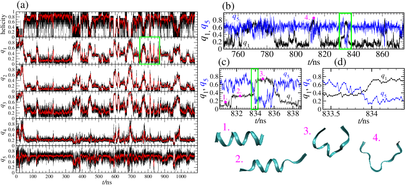
Fig. 1 shows the complete times series data for the simulated oligopeptide. In all five RCs and in the helicity data frequent switching between the folded state (large helicity and small values) and the unfolded state is observed, meaning that the simulation is converged and allows drawing conclusions on the folding and unfolding kinetics (further evidence is provided by the excellent comparison between straight MD and replica-exchange simulations, as shown in Fig. 6). The fine resolution data (Fig. 1, right panel) in terms of the RMS-deviation from the fully helical state, RC , suggest that an intermediate state and two barriers are present. As the snapshots indicate, in the fully helical state () roughly three -helical turns are stabilized by salt bridges between the Glu+-2 and Lys--6 and the Glu+-7 and Lys--11 residues, respectively. In the intermediate state () only one of the two salt bridges stabilizes two turns, while in the unfolded state () no bridge is present. Note that the characteristic transition time for unfolding of one helical turn, i.e. for the transition from to in (d), is roughly 200 ps and thus about 100 times shorter than the corresponding unfolding time in Fig. 3(e). While a high degree of correlation between different RCs can be inferred from Fig. 1, there is no one-to-one mapping, e.g., in Fig. 1(c) shows pronounced fluctuations in intervals where stays virtually constant.
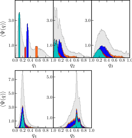
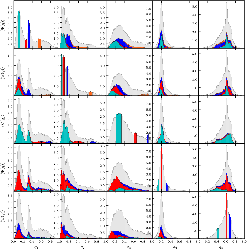
This is already evident from the average distribution function shown in Fig. 2 as a function of all different RCs. While the distribution in the leftmost panel as a function of shows three broad peaks (corresponding roughly to none, one and two intact salt bridges), clearly separated peaks are absent when is shown as a function of , , or . The reason is simple: states that are separated when, e.g., described by , are mixed when they are projected onto different RCs. This is demonstrated by the coloured regions in Fig. 2 that for correspond to pure states, i.e. narrow intervals of values. While for and the colored regions are smeared out but the ordering along the RC is preserved, for and the ordering is lost. This points to a fundamental difference between the RCs , that embody knowledge of the native state, and the RCs , which are purely geometric.
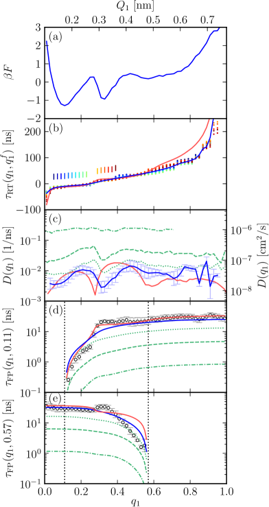
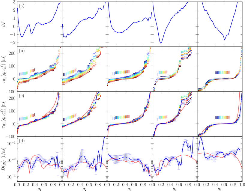
In Fig. 3 we focus on RC . The free energy profile in a) reveals the intermediate state and two barriers at and . Fig. 3(b) shows the roundtrip times for various final states as a function of , directly extracted from the simulation time series Supplement . The data sets are shifted vertically (which according to Eq. (9) is irrelevant for extracting ) to illustrate the predicted collapse onto a single mean round-trip time function . The smooth fit is shown as a blue curve. The collapse of for different is a strong check on the consistency of the FP approach. The red curve denotes the round-trip time from the Bayesian approach Hummer , obtained for optimized time interval and smoothing parameters and Supplement . Fig. 3(c) shows the diffusivity extracted from via Eq. (9) (blue curve). Most notably, varies considerably along : it is reduced by an order of magnitude around the intermediate state at and seems correlated with . The profile from the Bayesian approach (red curve) reproduces the coarse features of our round-trip approach with slight difference that will be discussed below. We stress that we have fitted the two parameters in the Bayesian approach, namely the time interval and the smoothing parameter, by a comparison with the simulation mean-first passage times (see Supplement for further details Supplement ). The diffusivity profiles resulting from the Bayesian approach sensitively depend on these parameters, and without such a comparison it is not easy to see what are sensible parameter values. This highlights an advantage of our method based on the round-trip time, since the only parameter is a smoothing factor that operates directly on the round-trip time, a physical observable, and sensible parameter values are straightforwardly estimated. The variance method Eq. (10) for lag time fs (upper green curve) overestimates by two orders of magnitude, yet for ps (lower green curve) approaches the results of the other two methods quite nicely. Thus for ps, is dominated by non-Markovian events that are unrelated to the long-time folding/unfolding dynamics; interestingly, this threshold time is similar to the transition time for helix unwrapping inferred from Fig. 1(d). In Figs. 3(d) and (e), we show MFP times for (folding) and (unfolding) calculated from Eq. (3) and the various profiles shown in (c). directly extracted from simulation data (circles) in Fig. 3(d) is most accurately reproduced by the Bayesian fitting approach (red curve), as expected since the probability distribution and thus the frequency of transitions is maximal in the range (see Fig. 2(a). The RT approach (blue curve) considers an equal balance of folding and unfolding events and consequently describes unfolding MFP times in Fig. 3(e) better. Noteworthy, the RT approach is simple to implement, directly works on the property one wishes to describe (namely folding/unfolding times) and has apart from the functional form of the fitted round-trip time no freely adjustable parameter. The combined deviations between simulation data and Fokker-Planck predictions in Figs. 3(d,e) are due to a combination of non-Markovian processes at short times and insufficient trajectory sampling.
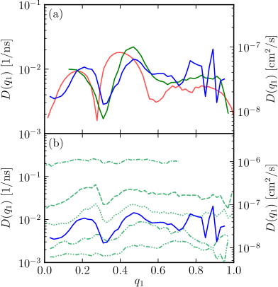
In Fig. 4(a) we compare the diffusivities based on the round-trip time approach (blue curve) and the Bayesian approach (red curve), already presented in Fig. 3(c), with results obtained from the MFP times via Eq. (5), shown as a green curve. For the fit we used a final state and considered folding events from to . It is seen that the three curves roughly coincide, which testifies to the robustness of methods for deriving diffusivities from folding times. In Fig. 4(b) we compare diffusivities from the variance method, Eq. (10), to the round-trip time method Eq. (9) (blue curve). Here we present results for for a wider range of lag times of fs, 20 ps, 200 ps, 2 ns and 10 ns (green curves, from top to bottom). It is seen that for lag times between ps and ns, agrees with the round-trip time approach. As already discussed, for smaller lag times is too large. For larger lag times loses structure and becomes too small, which has to do with the fact that at those times the peptides explores a considerable subsection of the free energy space and the effect of the energetic barriers encountered are spuriously accounted for by a reduction of the diffusivity. The situation is similar to the Bayesian approach: there is no a-priori way of knowing what the suitable parameter value for the lag time is, unless one compares to a physical observable, which might be the folding or round-trip time. In that case, however, a direct fitting of based on folding times as suggested by us seems more direct and transparent.
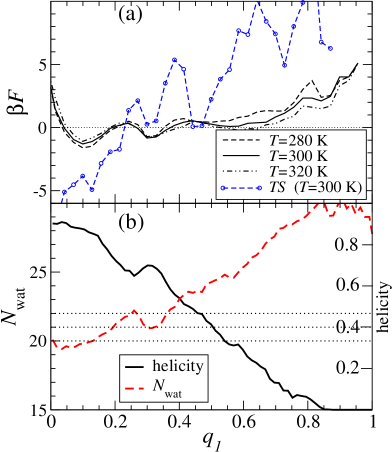
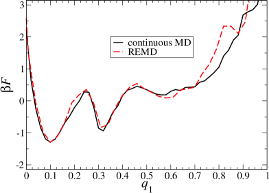
A free energy barrier, as exhibited by in Fig. 3(a), was argued to arise from a subtle compensation of energy and entropy effects, which both increase upon unfolding Wolynes . This scenario, developed in the context of lattice models, is basically confirmed by our explicit water simulations. In Fig. 5(a), we show free energy profiles at different temperatures from replica-exchange simulations. Indeed, the entropic contribution , estimated from the free energy difference between 280K and 320K, shows considerable numerical error but rises across the unfolding transition. In Fig. 5(b) we show the number of backbone-bound water molecules that have a distance to a backbone oxygen smaller than 0.35nm. Apart from the loss of one bound water molecule at (paralleled by a helicity increase), steadily rises from about in the folded state to in the unfolded state. So we conclude that the entropy increase upon unfolding results from a competition of water binding and conformational effects. The overall good comparison between the free energy profile from a standard MD simulation run (for a length of 1.1s) and results from a replica exchange MD simulation (trajectory length 22.5 ns and equilibrated with 32 replicas at different temperatures) at T=300K in Fig. 6 gives good evidence that the times series considered in our kinetic analysis is long enough.
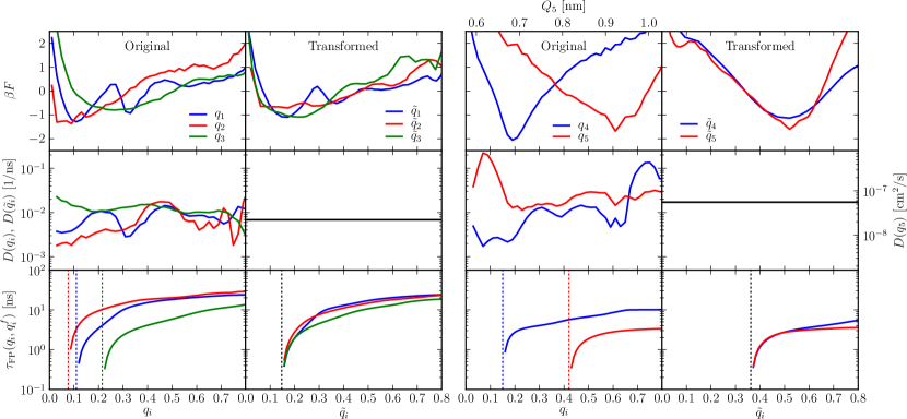
The appearance of a free energy barrier, as seen in in Fig. 3(a), is often interpreted as equivalent to exponential kinetics, which is not necessarily true as we will now discuss. In fact, even the presence of a free energy barrier depends on the specific RC employed and thus is a much less robust feature than often assumed: In Fig. 7 we show the free energy and diffusivity profiles of all five RCs. We separate RCs that embody knowledge of the native state and the unbiased RCs . In the columns ”Original” we use the bare RCs as defined in the Methods section, in the columns ”Transformed” we use rescaled RCs such that the diffusivities are constant, . Two features strike the eye:
i) Most diffusivity profiles are full of structure and vary substantially along the reaction path; it immediately transpires that a description of the folding kinetics without consideration of the diffusivity profile can fail.
ii) The profiles and vary considerably among different RCs. In fact, while shows pronounced barriers and an intermediate state, the profiles and are free of barriers: We conclude that the presence of barriers depends on the RC chosen. Do the kinetics within an effective Fokker-Planck description also vary among RCs, possibly showing exponential for some and non-exponential behavior for other RCs? While the free energy profiles as a function of the original RCs show large variations, the profiles after the transformation are quite similar (this is most striking for the radius of gyration, , and the end-to-end radius, ), and thus the kinetics as characterized by the MFP times in the bottom row are very similar. This at first surprising result can be easily rationalized: the round-trip method is designed to optimally reproduce the complete set of round-trip times and thus the slowest conformational transitions in the system. The different diffusivities and free energy profiles together uniquely determine the folding times. Assuming that different RCs yield a comparable separation of states into the unfolded and folded basins, it follows that the folding times must be very similar. This in fact holds for the RCs on the one hand and for the RCs on the other hand. Since after the rescaling the entire kinetic information is contained in the free energy profile, those profiles must be quite similar. It follows that the presence of a free energy barrier does not necessarily imply exponential kinetics; for that statement to be true the free energy barrier must persist after a RC transformation that makes the diffusivity profile flat. Although there are still differences among the free energy profiles for after the transformation, they are small enough that the kinetics are not particularly distinguished.
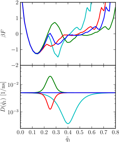
To highlight the implications of these results, we now turn the argumentation around. Consider a general RC transformation
| (12) |
that is assumed to be a monotonic function which implies that . This rescaling corresponds to a local stretching / compression of the RC around and via the reparametrization properties of the Fokker-Planck equation also modifies the diffusivity and the free energy profiles. In Fig. 8 we show three different rescaled and profiles, all generated via Eq. (12) from the RC for which is flat (shown in blue). Depending on the parameters we generate free energy profiles that either exhibit a more pronounced barrier (green curve), a reduced barrier (red curve), or a free energy profile where the position of the minimum is moved from the folded to the unfolded state (turquoise curve). We mention that by construction, the kinetics as characterized by the round trip or MFP time are invariant under this rescaling. What this figure demonstrates is that under a combined rescaling of and one can generate a bewildering variety of free energy curves which share the identical kinetics, meaning that the free energy profile without the diffusivity is not sufficient to even qualitatively predict protein folding kinetics.
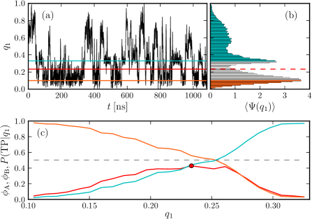
Much of the discussion in the preceding sections and the usage of one-dimensional RCs presumes that the reaction coordinates are “good” in the sense that i) the ensemble of transition states is assigned to a narrow region of RC values and ii) that the probability of finding a transition state in that region is maximal Bolhuis ; BestHummer2 . To make that notion more concrete, one introduces the splitting probabilities and for each value of the RC, where is the probability to reach, starting from RC value , region A before region B BestHummer2 . In the context of transition states, the regions A and B would denote regions corresponding to the folded and unfolded domains flanking the transition region. The splitting probabilities are normalized as
| (13) |
since eventually any state will diffuse out towards the boundaries. For a trajectory that passes through state there are four choices, it can be trajectory starting in A and returning to A, starting in B and returning B, starting in A and ending up in B or starting in B and ending in A. The respective probabilities are normalized as
| (14) |
For non-ballistic stochastic motion, the transition path probability , i.e. the probability that the trajectory connect regions A and B, can be maximally 1/2. A maximum close to 1/2 characterizes a good reaction coordinate, a significantly smaller number points to a bad reaction coordinate. In Fig. 9 we show a detailed reaction coordinate analysis for RC with a resolution of 25 bins in the range and using the full time resolution of 20 ps. In (a) we show again the complete time series and in (b) the corresponding probability distribution. Region A for is the folded region, region B for is a region where one helical turn is unfolded. In (c) we show the splitting probabilities and (orange and blue lines). The behavior is as expected, with the probabilities switching from zero to unity between the boundaries of the regions A and B, and a rather large slope in the region around . The maximum of the transition path probability (shown as a red curve) at a position means that is quite close to a perfect reaction coordinate and that the Fokker-Planck analysis performed in this paper is appropriate for long times on the order of folding and unfolding events. Note that is close to a minimum in the equilibrium distribution , see Fig.9b, at which position the free energy thus exhibits a maximum. This is coincidental, since as we have shown in Fig.8, one can easily change the free energy profile by a reaction-coordinate rescaling, which however leaves the splitting probabilities and the transition path probabilities invariant.
IV Conclusions
In the naive approach towards protein kinetics, folding times are deduced from the free energy profile alone. As has been argued before, BestHummer ; Wang ; BestHummer3 ; Onuchic such an approach is unreliable since for the simplest non-trivial folder, namely a single short -helix in explicit solvent, the diffusivity profile varies substantially along the folding path. Our variation comes out somewhat stronger than from similar simulations with implicit solvent, suggesting that explicit solvent further increases the importance of diffusivity inhomogeneities BestHummer . In fact, to match experimental folding times of simple alpha-helix forming oligo-peptides within solvent-implicit simulations, an overall correction factor to the time scales is typically appliedChowdhury ; Wang2 . A detailed microsopic justification for this is lacking; on the contrary, it has been shown that in many cases explicit solvent strongly influences the free energy landscape and introduces novel kinetic mechanisms that are completely absent in solvent-implicit simulationsZhou ; Pande2 . When extending the analysis to five different popular reaction coordinates, we find free energy and diffusivity profiles to vary substantially among different RC representations. Yet, the kinetics that follows from a Fokker-Planck description is largely independent of the RC chosen, if and only if is properly accounted for. A similar conclusion was reached recently based on coarse-grained, solvent-implicit simulations BestHummer3 . This means that a quasi-universal (i.e. RC independent) description of protein folding kinetics necessarily involves . For this quasi-universality to hold we have to distinguish between reaction coordinates that are based on the distance to the native state (such as ) and those that are purely geometric in nature (such as ). By considering generalized RCs and using the reparametrization invariance of the Fokker-Planck equation, we can design arbitrary profiles with no barrier at all, an enhanced barrier, or an interchange of the naive stable and unstable states. This means that the concept of a free energy profile is to some degree arbitrary, which might be relevant with regards to recent discussions in the experimental literature Gruebele ; Munoz ; Fersht2 . The kinetics, embodied in the folding time, and dependent on and , is less arbitrary.
Our simulations are for a single -helix fragment, one of the shortest oligopeptides which shows non-trivial folding. There is no reason to believe that for larger proteins the situation will simplify; we therefore argue that the diffusivity profile will be full of features and thus important in those more complicated situations as well. Our conclusions also apply to optimized or otherwise carefully selected RCs Bolhuis ; BestHummer2 ; Eric ; Orland ; Noe , since the reparametrization can be done for any RC and thus arbitrarily create, annihilate and shift barriers in the folding landscape (incidentally, RC turns out to be a quite good reaction coordinate according to the definition of Ref. BestHummer2 , as shown in Fig. 9). Our method of extracting the diffusivity profile via the mean-first-passage or round-trip time formalism can be easily applied to time series data from FRET or force-spectroscopic experiments, so an experimental test of our results is possible.
V Acknowledgements
We acknowledge support from the Deutsche Forschungsgemeinschaft (DFG) within SFB 863 and the Emmy-Noether-Programme (JD). The Leibniz Rechenzentrum (LRZ) Munich is acknowledged for supercomputing access.
References
- (1) E. Shaknovich, Chem. Rev. 106, 1559 (2006).
- (2) K. A. Dill, S. B. Ozkan, M. S. Shell, and T. R. Weikl, Annu. Rev. Biophys. 37, 289 (2008).
- (3) M. Oliveberg and P. G. Wolynes, Quart. Rev. Biophys. 38, 245 (2005).
- (4) A. Fersht, Structure and Mechanism in Protein Science (W.H. Freeman and Company, New York, 1999).
- (5) T. Cellmer, E. R. Henry, and J. Hofrichter, W. A. Eaton, Proc. Natl. Acad. Sci. 105, 18320 (2008).
- (6) A. Möglich, K. Joder, and T. Kiefhaber, Proc. Natl. Acad. Sci. 103, 12394 (2006).
- (7) B. Fierz, A. Reiner, and T. Kiefhaber, Proc. Natl. Acad. Sci. 106, 1057 (2009).
- (8) E. Rhoades, M. Cohen, B. Schuler, and G. Haran, J. Am. Chem. Soc. 126, 14686 (2004).
- (9) H. S. Chung, M. Louis, and W. A. Eaton, Proc. Natl. Acad. Sci. 106, 11837 (2009).
- (10) H. Dietz and M. Rief, Proc. Natl. Acad. Sci. 103, 1244 (2006).
- (11) H. Ma and M. Gruebele, Proc. Natl. Acad. Sci. 102, 2283 (2005).
- (12) P. Li, F. Y. Oliva, A. N. Naganathan, and V. Munoz, Proc. Natl. Acad. Sci. 106, 103 (2009).
- (13) F. Huang, L. Ying, and A. R. Fersht, Proc. Natl. Acad. Sci. 106, 16239 (2009).
- (14) C. J. Camacho and D. Thirumalai, Proc. Natl. Acad. Sci. 90, 6369 (1993).
- (15) D. Thirumalai, J. Phys. I France 5, 1457 (1995).
- (16) K. W. Plaxco, K.T. Simons, and D. Baker, J. Mol. Biol. 277, 985 (1998).
- (17) N. Agmon and J. J. Hopfield, J. Chem. Phys. 79, 2042 (1983).
- (18) N. D. Socci, J. N. Onuchic, and P. G. Wolynes, J. Chem. Phys. 104, 5860 (1996).
- (19) R. Du, V. S. Pande, A. Y. Grosberg, T. Tanaka, and E. S. Shakhnovich, J. Chem. Phys. 108, 334 (1998).
- (20) R. Zwanzig, Proc. Natl. Acad. Sci. 85, 2029 (1988).
- (21) R. Zwanzig, J. Chem. Phys. 97, 3587 (1992).
- (22) N.A. Denesyuk and J.D. Weeks, Phys. Rev. Lett. 102, 108101 (2009).
- (23) A. Alexander-Katz, H. Wada. R.R. Netz, Phys. Rev. Lett. 103, 028102 (2009).
- (24) R. B. Best and G. Hummer, Phys. Rev. Lett. 96, 228104 (2006).
- (25) J. Chahine, R.J. Oliveira, V.B.P. Leite, and J. Wang, Proc. Natl. Acad. Sci. 104, 14646 (2007).
- (26) R. B. Best and G. Hummer, Proc. Natl. Acad. Sci. 107, 1088 (2010).
- (27) S. Yang, J. N. Onuchic, A.E. Garcia, and H. Levine, J. Mol. Biol. 372, 756 (2007).
- (28) S. Marqusee and R. L. Baldwin, Proc. Natl. Acad. Sci. 84, 8898 (1987).
- (29) J. Dzubiella, J. Am. Chem. Soc. 130, 14000 (2008).
- (30) M. T. Woodside, P. C. Anthony, W. M. Behnke-Parks, K. Larizadeh, D. Herschlag, and S. M. Block, Science 314, 1001 (2006).
- (31) J. C. M. Gebhardt, T. Bornschlögl, and M. Rief, Proc. Natl. Acad. Sci. 107, 2013 (2010).
- (32) C. Hyeon and D. Thirumalai, J. Am. Chem. Soc. 130, 1538 (2008).
- (33) P. G. Bolhuis, D. Chandler, C. Dellago, and P. L. Geissler, Annu. Rev. Phys. Chem. 53, 291 (2002).
- (34) R. B. Best and G. Hummer, Proc. Natl. Acad. Sci. 102, 6732 (2005).
- (35) L. Maragliano, A. Fischer, E. Vanden-Eijnden, G. Ciccotti, J. Chem. Phys. 125, 024106 (2006).
- (36) M. Sega, P. Faccioli, F. Pederiva, G. Garberoglio, and H. Orland, Phys. Rev. Lett. 99, 118102 (2007).
- (37) F. Noe, C. Schütte, E. Vanden-Eijnden, L. Reich, T.R. Weikl, Proc. Natl. Acad. Sci. 106, 19011 (2009).
- (38) T. Ghosh, S. Garde, and A. E. Garcia, Biophys. J. 85, 3187 (2003).
- (39) D. A. Case, AMBER 9.0 software, University of California, San Francisco (2006).
- (40) W. Kabsch and D. Sander, Biopolymers 22, 2577 (1983).
- (41) P. Hänggi, P. Talkner, and M. Borkovec, Rev. Mod. Phys. 62, 251 (1990).
- (42) G. Hummer, New J. Physics, 7, 34 (2005).
- (43) G. H. Weiss, Adv. Chem. Phys. 13, 1 (1966).
- (44) J.O. Ramsay, G. Hooker, S. Graves, Functional Data Analysis with R and MATLAB (Springer, Berlin, 2009).
- (45) Y.M. Rhee and V.S. Pande, J. Phys. Chem. B 109, 6780 (2005).
- (46) S.V. Karplus and M. Karplus, Proc. Natl. Acad. Sci. 105, 13841 (2008).
- (47) S. Chowdhury, W. Zhang, C. Wu, G. Xiong, Y. Duan, Biopolymers 68, 63 (2003).
- (48) W.-Z. Wang, T. Lin, Y.-C. Sun, J. Phys. Chem. B 111, 3508 (2007).
- (49) R. Zhou, Proteins: Structure, Function and Genetics 53, 148 (2003).
- (50) Y.M. Rhee, E.J. Sorin, G. Jayachandran, E. Lindahl, and V.S. Pande, Proc. Natl. Acad. Sci. 101, 6456 (2004).
- (51) Supplemental Information.
Supplement to: “How the diffusivity profile reduces the arbitrariness of protein folding free energies”
M. Hinczewski, Y. von Hansen, J. Dzubiella, R. R. Netz
S.1 Mapping between reaction coordinates
Fig. 1 shows in the columns the average distribution function as a function of all five different RCs considered in the main text. In each row the coloured regions denote identical subsets of states and are chosen to correspond to pure states for one reaction coordinate. While among the RCs and among the RCs the ordering of the coloured regions is preserved, this ordering is lost between those two groups. This points to a fundamental difference between the RCs , that embody knowledge of the native state, and the RCs , which are purely geometric.
S.2 Extracting the diffusivity profile
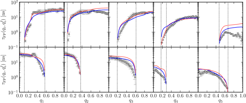
In Fig. 2 we show the free energy profiles, the round-trip times and the diffusivity profiles of all five reaction coordinates. In Fig. 3 we show the mean-first passage times for folding and unfolding events for all reaction coordinates, as extracted from the fitted diffusivity profiles and the Fokker-Planck description. The final states were chosen such that of the probability distribution is contained in the range (folding), or (unfolding). The noise and non-monotonicity in the curves extracted from the simulation data are due to the statistical effects of insufficient trajectory sampling (particularly at the edges of the free energy landscape) and time discretization.
S.3 Determining Diffusivity Profiles by Bayesian Inference
We briefly review the optimization method introduced in Ref. Hummer2005 , and used previously to extract diffusivity profiles for protein folding dynamics in implicit solvent Best2006 .
S.3.1 Master equation approach
When discretized in reaction coordinate space, the FP equation takes the form of a master equation Bicout1998
| (S.1) |
where the probability of being in bin is denoted by , the bin width is , the bin index ranges from to , and the transition rate from bin to bin is . The rates fulfill detailed balance, i.e. , where the equilibrium probability of each bin is denoted by ; the loss in bin is caused by transitions to neighboring bins, i.e. . The rates in the master equation S.1 are related to the free energy and the diffusivity profile in the FP equation via:
| (S.2) |
| (S.3) |
with being the diffusivity between the bins. For bins the system is consequently characterized by independent parameters: rates for transitions from the neighboring bin on the right hand side and equilibrium probabilities .
S.3.2 Bayesian analysis of trajectories
In a system described by Eq. S.1 the conditional probability of landing in bin in time given a start in bin is:
| (S.4) |
where is the matrix with entries . In our case is tridiagonal and the transition probabilities are easily obtained numerically by diagonalization of the symmetrized matrix defined by the entries Bicout1998 ; Hummer2005 . For a process described by Eq. S.1, the likelihood of observing a certain sequence with transitions at equidistant time intervals is:
| (S.5) |
where is the total number of transitions from to observed along the trajectory and the time intervals . Bayesian inference (BI) can be used to determine the underlying free energy and diffusivity profile from a stochastic trajectory. Bayes’ theorem states that for a given trajectory () the probability of certain parameters to be correct is:
| (S.6) | |||||
where is the likelihood of Eq. S.5; in our case the prior just depends on the diffusivity profile , penalizing large deviations of the diffusivity at adjacent grid points.
S.3.3 Optimization procedure
A standard simulated annealing scheme is used to optimize the probability in Eq. S.6 by iterative variation of the parameters of the system. The quantity to be minimized is the “energy” defined by:
| (S.7) |
At each step the parameters and are slightly perturbed giving rise to a new configuration with energy , which is always accepted for and accepted with probability for ; the “temperature” of the system is subsequently lowered until the optimized and are reached. Several independent simulated annealing runs are performed; variations in the results obtained in different runs allow drawing conclusions on the quality of the estimate and the suitability of the process for a FP type description.
S.3.4 Dependence of on the time interval and the smoothing parameter
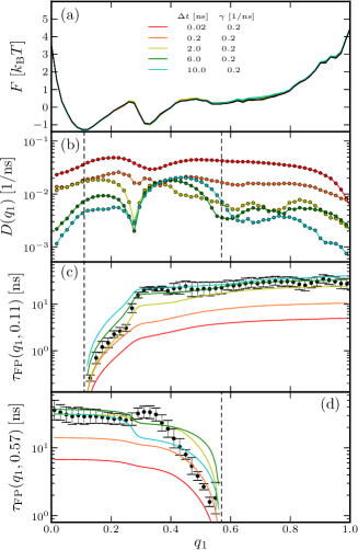
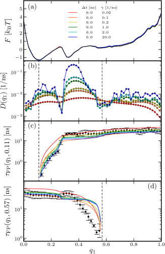
The Bayesian optimization method is applied to the dynamics of the reaction coordinate . In Fig. S.4 we compare results obtained for different time intervals ; in Fig. S.5 results for different values of the smoothing parameter weighting the prior in Eq. S.6 are shown.
We show results for bins along the RC, and show average values of and from independent optimization runs. Though being a fit quantity, the free energy profile does not significantly differ from obtained from the equilibrium analysis of the trajectory (black lines in the upper panel of the figures). We note that the diffusivity profile is strongly sensitive on the time interval : while almost identical profiles like in the variance method analysis are obtained for , the diffusivity subsequently decreases for larger . The parameter can compensate insufficient sampling by externally requiring a smoothness of the diffusivity; however, strong external constraints corresponding to low -values tend to erase any structure in .
Reasonable choices of the parameters and are not evident a priori — to ensure that the long-time dynamics are correctly reproduced by the optimization result, we compute the position dependent MFP times for a folded state () and an unfolded one () for each of the optimized diffusivity profiles and compare these curves to the one directly extracted from the simulation data. This comparison shows that in our case and are sensible values.
References
- (1) G. Hummer. Position-dependent diffusion coefficients and free energies from Bayesian analysis of equilibrium and replica molecular dynamics simulations. New J. Phys., 7, 2005.
- (2) R. B. Best and G. Hummer. Diffusive model of protein folding dynamics with Kramers turnover in rate. Phys. Rev. Lett., 96(22), 2006.
- (3) D. J. Bicout and A. Szabo. Electron transfer reaction dynamics in non-Debye solvents. J. Chem. Phys., 109(6):2325–2338, 1998.
- (4) G. Hummer. From transition paths to transition states and rate coefficients. J. Chem. Phys., 120(2):516–523, 2004.
- (5) R. B. Best and G. Hummer. Reaction coordinates and rates from transition paths. Proc. National Acad. Sciences United States Am., 102(19):6732–6737, 2005.