Coupled multimode optomechanics in the microwave regime

Abstract

The motion of micro- and nanomechanical resonators can be coupled to electromagnetic fields. This allows to explore the mutual interaction and introduces new means to manipulate and control both light and mechanical motion. Such optomechanical systems have recently been implemented in nanoelectromechanical systems involving a nanomechanical beam coupled to a superconducting microwave resonator. Here, we propose optomechanical systems that involve multiple, coupled microwave resonators. In contrast to similar systems in the optical realm, the coupling frequency governing photon exchange between microwave modes is naturally comparable to typical mechanical frequencies. For instance this enables new ways to manipulate the microwave field, such as mechanically driving coherent photon dynamics between different modes. In particular we investigate two setups where the electromagnetic field is coupled either linearly or quadratically to the displacement of a nanomechanical beam. The latter scheme allows to perform QND Fock state detection. For experimentally realistic parameters we predict the possibility to measure an individual quantum jump from the mechanical ground state to the first excited state.

Introduction. - Significant interest in the interaction and dynamics of systems comprising micro- and nanomechanical resonators coupled to electromagnetic fields, as well as the prospect to eventually measure and control the quantum regime of mechanical motion, has stimulated the rapidly evolving field of optomechanics (see Marquardt and Girvin (2009) for a recent review). In the standard setup, the light field, stored inside an optical cavity, exerts a radiation pressure force on a movable end-mirror whose motion changes the cavity frequency and thus acts back on the photon dynamics. This way, the photon number inside the optical mode is linearly coupled to the displacement of a mechanical object. Beyond the standard approach, new developments have introduced optical setups with multiple coupled light and vibrational modes pointing the way towards integrated optomechanical circuits Thompson et al. (2008); Li et al. (2008); Eichenfield et al. (2009, 2009); Anetsberger et al. (2009). These systems allow to study elaborate interactions between mechanical motion and light such as mechanically driven coherent photon dynamics that introduces the whole realm of driven two- and multi-level systems to the field of optomechanics Heinrich et al. (2010). Coupled multimode setups furthermore allow to increase measurement sensitivity Dobrindt and Kippenberg (2010) and enable fundamentally different coupling schemes. Accordingly, recent experiments achieved coupling the photon number to the square and quadruple of mechanical displacement Thompson et al. (2008); Sankey et al. (2010). Such different coupling schemes are needed, for instance, to afford quantum non-demolition (QND) Fock state detection of a mechanical resonator Thompson et al. (2008); Braginsky et al. (1980, 1992); Jayich et al. (2008).

Besides optics, recent progress has made it possible to realize optomechanical systems in the microwave regime Regal et al. (2008); Hertzberg et al. (2010). In this case the optical cavity is replaced by a superconducting microwave resonator whose central conductor capacitively couples to the motion of a nanomechanical beam. This optomechanical approach constitutes a new path to perform on-chip experiments measuring and manipulating nanomechanical motion that adds to electrical concepts using single electron transistors Knobel and Cleland (2003); LaHaye et al. (2004); Naik et al. (2006), superconducting quantum interference devices Etaki et al. (2008); Buks et al. (2008), driven RF circuits Brown et al. (2007) or a Cooper-pair-box LaHaye et al. (2009); O/’Connell et al. (2010). One advantage of on-chip optomechanics is to use standard bulk refrigerator techniques in addition to laser cooling schemes Teufel et al. (2008, 2008). This recently enabled cooling a single vibrational mode close to the quantum mechanical ground state Rocheleau et al. (2010). Furthermore, nonlinear circuit elements can be integrated. This afforded ultra-sensitive displacement measurements with measurement imprecision below that at the standard quantum limit Teufel et al. (2009).

Here we go beyond single mode systems, that have been considered for optomechanics in the microwave regime so far, and propose setups with coupled microwave resonators. For these systems, the coupling frequency between microwave modes turns out to be comparable to the mechanical frequency. This has several implications both for the classical and the prospective quantum regime. As an example, focusing on the currently in experiments accessible regime of classical motion, we demonstrate how this allows to manipulate the microwave field in terms of mechanical driving.

Two-resonators setup with linear mechanical coupling. - We consider the coplanar device geometries depicted in Fig. 1a with two identical superconducting microwave resonators $a_{L}$, $a_{R}$.

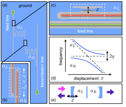
Figure 1: Schematic device geometry for two superconducting microwave resonators $a_{L}$, $a_{R}$ with a nanomechanical beam coupled to $a_{L}$. (a) The two resonators (each of length $d$) are coupled to external feed and transmission lines (green). (b) The central conductors of $a_{L}$ and $a_{R}$ (red) capacitively couple due to a small region of length $d_{g}$ where the resonators adjoin. (c) At the other end of $a_{L}$ a small mechanical beam, connected to ground (blue), is placed. Its displacement $x$ affects the line capacitance of resonator $a_{L}$ changing its resonance frequency. (d) System’s resonance frequency as function of displacement: the beam’s displacement $x$ linearly changes the bare mode frequency of $a_{L}$ while the one of $a_{R}$ is unaffected (dashed). Due to the coupling $g$ between modes there is an avoided crossing $2g$ in the eigenfrequencies (blue). (e) Analogous optical setup: a static, dielectic membrane, placed inside a cavity with a movable mirror, couples two separate optical modes $a_{L}$, $a_{R}$.

The central conductors of $a_{L}$ and $a_{R}$ are assumed to adjoin for a length $d_{g}$ that is much smaller than the total wave guides’ length $d$ [Fig. 1b]. A nanomechanical beam, connected to the ground plane, is placed at the other end of $a_{L}$ [Fig. 1c]. Its motion in terms of displacement $x$ changes the line capacitance $c$ (capacitance per unit length) between the central conductor and the ground plane in a small region. In the following, we will derive and discuss the Hamiltonian for the system depicted in Fig. 1 starting from a single microwave resonator whose line capacitance is changed due to the motion of a mechanical beam [Fig. 1b] Regal et al. (2008); Teufel et al. (2008); Rocheleau et al. (2010).

Single MW resonator coupled to a nanomechanical beam. - We concentrate on one of the microwave resonators in Fig. 1. The Lagrangian of an electric circuit can be conveniently expressed in terms of a flux variable $\phi(x,t)\equiv\int_{-\infty}^{t}d\tau\,V(x,\tau),$ where $V(x,t)=\partial_{t}\phi(x,t)$ is the voltage on the transmission line at position $x$ and time $t$, see for instance Devoret (1995). For a finite length microwave resonator with line inductance $l$ and line capacitance $c$ (both per unit length), the corresponding Euler-Lagrange equation yields a wave equation with speed $v=\sqrt{1/lc}$. Using appropriate boundary conditions, $\phi(x,t)$ can be expanded into normal modes $\phi_{k}$, see Blais et al. (2004). The Lagrangian reads $\mathcal{L}=\sum_{k}[\frac{c}{2}\dot{\phi}_{k}^{2}+\frac{1}{2l}\left(\frac{k\pi}{d}\right)^{2}\phi_{k}^{2}]$ and the microwave resonator possesses resonance frequencies $\omega_{k}=k\pi v/d$. The Hamiltonian is obtained by Legendre transformation using the canonically conjugated momentum $\pi_{k}=c\dot{\phi}_{k}$. Quantizing the system by introducing creation and annihilation operators $a_{k}^{\dagger}$, $a_{k}$ for the individual modes $k$, with $[a_{k},\,a_{k^{\prime}}^{\dagger}]=\delta_{k,k^{\prime}}$, the Hamiltonian is a sum of harmonic oscillators, $\sum_{k}\hbar\omega_{k}a_{k}^{\dagger}a_{k}$, where we neglected the vacuum energy.

For the resonator $a_{L}$ in Fig. 1, the motion of the mechanical beam will change the line capacitance $c$ at the end of the wave guide. If we denote the total capacitance between the central conductor and the beam by $C_{b}$ and define the optomechanical frequency pull per displacement, $\epsilon_{k}=-\partial\omega_{k}/\partial x$, we find

$$\epsilon_{k} = \frac{\partial C_{b}}{\partial x}\cdot Z\cdot\omega_{k}^{2}/\left(2\pi k\right),$$ (1)

where we used the line impedance $Z=\sqrt{l/c}$. Up to linear order in $x$, the Hamiltonian for a single microwave resonator coupled to a nanomechanical beam reads $\mathcal{H}=\sum_{k}\hbar\left(\omega_{k,0}-\epsilon_{k}x\right)a_{k}^{\dagger}a_{k}$.

Coupled MW resonators. - We now turn to the coupled resonator setup in Fig. 1. As the length $d_{g}$ of the region where $a_{L}$ and $a_{R}$ adjoin is much smaller than the resonators’ length $d$, the capacitive coupling between both central conductors can be considered in terms of a constant, total capacitance $G$. We briefly switch to a discretized description. If we neglect the motion of the nanomechanical beam the circuit diagram looks as depicted in Fig. 2, where the flux variable $\phi(x,t)$ is discretized as $\phi_{n}(t)$ at position $x=na$, with $a$ being the constant spacing between nodes. For each individual node, an equation of motion can be written down Devoret (1995). From this, taking into account appropriate boundary conditions for $a\rightarrow 0$, the continuous version of the corresponding Lagrangian is found to be

$$\mathcal{L} = \sum_{k}\left[\frac{c}{2}\dot{\phi}_{L,k}^{2}-\frac{1}{2l}\left(\frac{k\pi}{d}\right)^{2}\phi_{L,k}^{2}\right]$$ (2)

$$+ \sum_{k}\left[\frac{c}{2}\dot{\phi}_{R,k}^{2}-\frac{1}{2l}\left(\frac{k\pi}{d}\right)^{2}\phi_{R,k}^{2}\right]$$

$$+ \frac{G}{d}\left(\sum_{k}\dot{\phi}_{R,k}-\sum_{k}\dot{\phi}_{L,k}\right)^{2},$$

where $\phi_{L,k}$, $\phi_{R,k}$ refer to the individual normal modes of the left and right resonator, respectively. The first two terms describe two separate wave guides, while the last term characterizes the coupling between both.

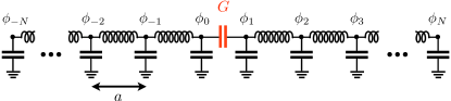
Figure 2: Discretized circuit diagram for the system depicted in Fig. 1 without nanomechanical beam. The two central conductors are coupled via a total capacitance $G$. $l$ and $c$ are the line inductance and capacitance, respectively. $a$ is the spacing between discrete points.

To transform to the Hamiltonian, we consider the canonically conjugated momentum $\pi_{L[R],k}=\partial L/\partial\dot{\phi}_{L[R],k}=c\dot{\phi}_{L[R],k}\mp 2\frac{G}{d}(\sum_{k}\dot{\phi}_{R,k}-\sum_{k}\dot{\phi}_{L,k})$. In the following we will restrict to a single mode in each resonator ($k=1$), and drop the label referring to the mode index. For $G/d\ll c$ (see discussion below), we can simplify the expression for $\pi_{L[R],k}$ and consider $\pi_{L[R],k}=c\dot{\phi}_{L[R],k}$. The first two terms of (2) transform into two harmonic oscillators of frequency $\omega_{L}$ and $\omega_{R}$. For the coupling we have to consider $(\dot{\phi}_{R}-\dot{\phi}_{L})^{2}$ with $\dot{\phi}_{L[R]}=\pi_{L[R]}/c=i\sqrt{\frac{\hbar\omega_{L[R]}}{2c}}\left(a_{L[R]}^{\dagger}-a_{L[R]}\right)$, see Blais et al. (2004). Using rotating wave approximation, we find the Hamiltonian,

$$\mathcal{H} = \hbar\omega_{L}\left(1-\frac{G}{dc}\right)a_{L}^{\dagger}a_{L}+\hbar\omega_{R}\left(1-\frac{G}{dc}\right)a_{R}^{\dagger}a_{R}$$

$$+ \hbar\sqrt{\omega_{L}\omega_{R}}\frac{G}{dc}\left(a_{L}^{\dagger}a_{R}+a_{R}^{\dagger}a_{L}\right),$$

where we neglected the vacuum energy. Note that none of the resonators in Fig. 1 is short-circuited such that there are voltage antinodes at both ends of each resonator allowing to have maximal coupling between $a_{L}$ and $a_{R}$, as well as to the feed and transmission line.

The coupling between the resonators has two effects. First, both frequencies $\omega_{L}$, $\omega_{R}$, originally defined for uncoupled modes, are lowered by a constant value. In the following, this shift of frequency is neglected by simply redefining the resonators’ frequencies. More important is the coupling between modes in terms of the coupling frequency

$$g = \sqrt{\omega_{L}\omega_{R}}\frac{G}{dc}.$$ (3)

Finally we take into account the motion of the nanomechanical beam changing the left mode’s bare eigenfrequency $\omega_{0}$ in the way discussed above, $\omega_{L}(x)=\omega_{0}-\epsilon x$ (see Eq. (1) with $k=1$). The final Hamiltonian for the system depicted in Fig. 1 then reads

$$\mathcal{H} = \hbar\left(\omega_{0}-\epsilon x\right)a_{L}^{\dagger}a_{L}+\hbar\omega_{0}a_{R}^{\dagger}a_{R}$$ (4)

$$+ \hbar g\left(a_{L}^{\dagger}a_{R}+a_{R}^{\dagger}a_{L}\right).$$

In principle, according to (3) with $\omega_{L}(x)$, the coupling frequency $g$ depends on displacement $x$. However, for typical parameters the dependence is negligible and $g$ can be considered to be constant. The resonance frequency of (4) is depicted in Fig. 1d.

Coupling frequency comparable to the mechanical frequency ($g\simeq\Omega$). - Given Eq. (3), the coupling frequency between the two resonator modes reads $g/\omega_{0}=(c_{g}/c)\cdot(d_{g}/d)$, where we defined the coupling line capacitance $c_{g}=G/d_{g}$ along the length of the coupling region $d_{g}$. In general, $c_{g}$ will be much smaller than the line capacitance between each central conductor and the ground plane $c$: first of all, the distance between the two central conductors is significantly larger than the distance between a single conductor and the adjacent ground plane. Second, the capacitance between the central strip lines is shielded by the grounded region in between. Here we crudely assume $c_{g}/c=10^{-2}$. For $d$ in the cm range and $d_{g}\simeq 0.1\text{mm}$ ($d_{g}$ is chosen such that a several $10\,\mu\text{m}$ long nanomechanical beam can be fabricated in between the region where the resonators align), we have $d_{g}/d=10^{-2}$ and the coupling between modes is $g/\omega_{0}=10^{-4}$ where $\omega_{0}$ will be in the GHz range. Common eigenfrequencies of nanomechanical beams are $\Omega=100\text{ \text{kHz}}$ - $10\text{ MHz}$. Hence, due to their much smaller photon frequency, coupled multimode optomechanical systems in the microwave regime naturally possess coupling frequencies in the range of typical mechanical frequencies ($g\simeq\Omega$). The relevance of this regime for instance to realize all kinds of driven two- and multi-level photon dynamics in optomechanical systems has been pointed out in Heinrich et al. (2010).

Transmission spectrum. - As an example to emphasize the characteristics of coupled optomechanical systems in the microwave regime and to demonstrate implications of $g\simeq\Omega$ even in the presently accessible regime of classic mechanical motion, we will discuss how the microwave field in the setup of Fig. 1 can be manipulated in terms of mechanical driving (see Unterreithmeier et al. (2009) for a universal mechanical actuation scheme). Experimentally, the impact can be most easily observed in terms of the transmission spectrum. We assume the left resonator $a_{L}$ to be driven at frequency $\omega_{L}$ via the feed line, while the transmission down the transmission line is recorded. We consider the coupling of the left (right) resonator to the feed (transmission) line in terms of the the resonators’ decay rate $\kappa$. Given the Hamiltonian (4), using input/output theory, the equation of motion for the averaged fields $\alpha_{L}=\langle a_{L}\rangle$, $\alpha_{R}=\langle a_{R}\rangle$ read

$$\frac{d}{dt}\alpha_{L} = \frac{1}{i}\left(-\epsilon x(t)\alpha_{L}+g\alpha_{R}\right)-\frac{\kappa}{2}\alpha_{L}-\sqrt{\kappa}b_{L}^{in}(t)$$

$$\frac{d}{dt}\alpha_{R} = \frac{1}{i}g\alpha_{L}-\frac{\kappa}{2}\alpha_{R},$$ (5)

where $b_{L}^{in}(t)=e^{-i\Delta_{L}t}b^{in}$ describes the electromagnetic drive along the feed line with amplitude $b^{in}$ and frequency $\omega_{L}$. Here we used a rotating frame with laser detuning from resonance $\Delta_{L}=\omega_{L}-\omega_{0}$. The transmission $T(t)=\kappa\langle a_{R}^{\dagger}(t)a_{R}(t)\rangle/\left(b^{in}\right)^{2}$ can be expressed as

$$T(t)=\kappa^{2}\left|\int_{-\infty}^{t}G(t,t^{\prime})e^{-i\Delta_{L}t^{\prime}-(\kappa/2)(t-t^{\prime})}\,dt^{\prime}\right|^{2},$$ (6)

where the phase comprises the feed line’s drive and resonators’ decay, while the Green’s function $G(t,t^{\prime})$ describes the amplitude for a photon to enter the left resonator’s mode $a_{L}$ at time $t^{\prime}$ and to be found in the right one $a_{R}$ later at time $t$.

We take into account two scenarios: first, the beam is at rest given a constant displacement $x(t)=x_{0}$; second, the beam is mechanically driven to oscillate with amplitude $A$ and frequency $\Omega$ around the mean position $x_{0}$, $x(t)=x_{0}+A\cos(\Omega t)$. Fig. 3a shows numerical results of the transmission spectrum without mechanical driving. The spectrum corresponds to the system’s resonance frequency depicted in Fig. 1d where the resonance width is set by the resonators’ decay rate $\kappa$.

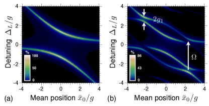
Figure 3: Transmission spectrum for the setup depicted in Fig. 1 for resonators’ decay rate $\kappa=0.1g$: density plot for the time-averaged transmission depending on mean mechanical displacement $\bar{x}_{0}=\epsilon x_{0}$, and frequency detuning $\Delta_{L}=\omega_{L}-\omega_{0}$ of the feed line’s microwave drive at $\omega_{L}$ ($\omega_{0}$ denotes the left mode’s bare frequency for $x=0$). (a) Without mechanical drive ($x(t)=x_{0}$); the spectrum is given by the resonance frequency depicted in Fig. 1d. (b) For mechanical driving ($x(t)=A\cos(\Omega t)+x_{0}$) with amplitude $\bar{A}=\epsilon A=1.5\Omega$ and frequency $\Omega=3g$; mechanical sidebands displaced by $\Omega$ appear and intersect the original photon branches where, due to mechanically driven Rabi dynamics, high transmission and additional anticrossings arise. The gap $2g_{1}$ is determined by the Bessel function $J_{1}$ according to $2g_{1}=2gJ_{1}(\bar{A}/\Omega)$.

In contrast, Fig. 3b shows the transmission including mechanical driving with $\Omega=3g$, i.e. $g\simeq\Omega$ being characteristic for coupled microwave optomechanics.

To understand the main features of Fig. 3b we note that, in general, two processes are involved to observe transmission, see (6): first, the left resonator $a_{L}$ must be excited by the electromagnetic drive $b_{L}^{in}(t)=e^{-i\Delta_{L}t}b^{in}$; second, the internal dynamics must be able to transfer photons from $a_{L}$ to $a_{R}$. From (5) the solution $G(t,t^{\prime})$ can be found to be

$$G(t,t^{\prime})=\tilde{\alpha}_{R}(t,t^{\prime})e^{-i\phi(t^{\prime})}$$ (7)

where $\phi(t^{\prime})=(\bar{A}/\Omega)\sin(\Omega t^{\prime})$ and $\tilde{\alpha}_{R}(t,t^{\prime})$ is a solution to the driven two state problem

$$\frac{d}{dt}\left(\begin{array}[]{c}\tilde{\alpha}_{L}\\ \tilde{\alpha}_{R}\end{array}\right)=\frac{1}{i}\left(\begin{matrix}-\bar{x}_{0}&ge^{-i\phi(t)}\\ ge^{+i\phi(t)}&0\end{matrix}\right)\left(\begin{array}[]{c}\tilde{\alpha}_{L}\\ \tilde{\alpha}_{R}\end{array}\right),$$ (8)

with $t\geq t^{\prime}$ and initial condition $\tilde{\alpha}_{L}(t^{\prime},t^{\prime})=1$, $\tilde{\alpha}_{R}(t^{\prime},t^{\prime})=0$. Note that we expressed displacement in terms of frequency; $\bar{A}=\epsilon A$, $\bar{x}_{0}=\epsilon x_{0}$. For $\bar{A}\neq 0$, in addition to the electromagnetic drive (see $e^{-i\Delta t^{\prime}}$ in (6)), the mechanical driving can excite $a_{L}$ in terms of multiples of the mechanical frequency $m\Omega$. This mechanical excitation is described by the phase factor $e^{-i\phi(t^{\prime})}=\sum_{m}J_{m}(\bar{A}/\Omega)e^{-im\Omega t^{\prime}}$ in (7) and leads to mechanical sidebands in the spectrum [cf. Fig. 3b]. Note that the individual process $m\Omega$ is described by a Bessel function $J_{m}(\bar{A}/\Omega)$ and can be tuned by the driving strength. Beyond the modified excitation, the driving significantly changes the internal dynamics of the microwave fields, see Eq. (8). In particular the mechanical motion can initiate mechanically driven Rabi dynamics exchanging photons between $a_{L}$ and $a_{R}$ that leads to high transmission if the mechanical drive at $\Omega$ is in resonance with the modes’ frequency difference. For sufficiently strong driving, the mechanically assisted process leads to additional anticrossings in the spectrum resembling Autler-Townes splittings known from quantum optics (see marker in Fig. 3b). From Eq. (8) we find that the spacing of this first additional splitting scales according to $2gJ_{1}(\bar{A}/\Omega)$ and can likewise be tuned by the mechanical driving strength. All this illustrates how, due to $g\simeq\Omega$, the microwave field can extensively be manipulated by mechanical motion in terms of mechanically driven coherent photon dynamics.

Coupling to the square of displacement. - We present a modified scheme comprising coupled microwave resonators that allows to couple the photon number to the square of mechanical displacement [Fig. 4a-b].

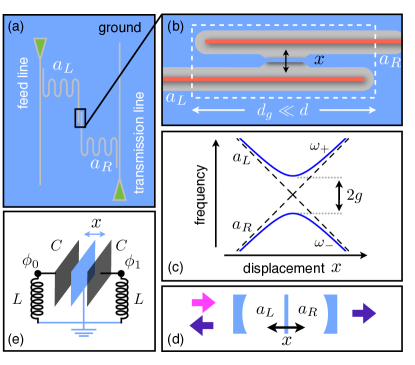
Figure 4: Schematic device geometry for two microwave resonators $a_{L}$, $a_{R}$ with a nanomechanical device coupled to both of them. (a) Two stripline resonators (each of length $d$) are coupled to external feed and transmission lines (green). The central conductors of $a_{L}$, $a_{R}$ (red) are capacitively coupled in a small region of length $d_{g}$ where the wave guides adjoin. (b) Between the two resonators a small mechanical beam, connected to ground (blue), is placed. Its displacement $x$ affects the line capacitance of both, $a_{L}$ and $a_{R}$. (c) System’s resonance frequency as function of displacement: the beam’s displacement linearly changes the bare modes’ frequency of $a_{L}$ and $a_{R}$ (dashed). Due to the coupling $g$ between the resonators, there is an avoided crossing $2g$ in the eigenfrequencies $\omega_{\pm}$ (blue). (d) Analogous optical setup with a movable dielectric membrane placed in the middle of a cavity Thompson et al. (2008). (e) Schematic realization with two microwave LC circuits where a central plate is grounded and resonates against two others that build the LC circuits. In the notation of Fig. 2 we get for the coupling frequency $g=\omega_{LC}G/C$ with $\omega_{LC}=1/\sqrt{LC}$.

In contrast to the setup in Fig. 1, here the nanomechanical beam is placed in the region between the two resonators, such that its motion affects both simultaneously [Fig. 4b]. While for a given displacement $x$, the line capacitance $c$ of the first resonator is increased, the one of the second wave guide is decreased and vice versa. According to our previous results, using the notation from above, the Hamiltonian for this setup reads

$$H = \hbar\left(\omega_{0}-\epsilon x\right)a_{L}^{\dagger}a_{L}+\hbar\left(\omega_{0}+\epsilon x\right)a_{R}^{\dagger}a_{R}$$ (9)

$$+ \hbar g\left(a_{L}^{\dagger}a_{R}+a_{R}^{\dagger}a_{L}\right),$$

where $g=\omega_{0}c_{g}d_{g}/cd$, see (3) and (4).

Fig. 4c illustrates the system’s resonance frequency $\omega_{\pm}(x)=\omega_{0}\pm\sqrt{g^{2}+(\epsilon x)^{2}}$ as function of displacement. Naturally all the characteristics of coupled multimode optomechanics in the microwave regime, that have been discussed above, apply. In particular the hyperbola-shaped avoided level crossing allows to realize Landau-Zener transitions and the dynamics of Landau-Zener-Stueckelberg oscillations in the light field of a microwave setup. At the extrema of $\omega_{\pm}(x)$ the Hamiltonian allows an exclusive coupling to the square of mechanical displacement $x^{2}$. Thus, in the following, we investigate the prospects to perform QND Fock state detection using this microwave setting.

$\epsilon$ [MHz/nm]	$m$ [pg]	$\Omega/2\pi$ [MHz]	$Q/10^{5}$	$\kappa/\Omega$	$g/2\pi$ [MHz]	$P_{in}$ [pW]	$x_{0}$ [pm]	$n_{add}$	$T$ [mK]	$\Sigma$
$65$	$10$	$11$	3.5	$1/70$	0.5	200	0.5	1	20	1.0
70	10	11	5.0	1/100	0.5	50	0.5	1	20	1.2

Table 1: Two sets of experimental parameters that would allow to observe an individual quantum jump from the mechanical ground state to the first excited state, with a signal-to-noise ratio $\Sigma\geq 1$. Further parameter $\omega_{c}/2\pi=5\text{ GHz}$.

Fock state detection. - In principle, an exclusive coupling of the photon number to $x^{2}$ allows to perform QND Fock state detection and to observe quantum jumps of a mechanical resonator Braginsky et al. (1980, 1992). Indeed the Hamiltonian (9) corresponds to the one found for an optical setup (see Fig. 4d), that generated a lot of interest in this regard Thompson et al. (2008); Jayich et al. (2008). We focus on one microwave mode with annihilation operator $a$ and expand the resonance frequency $\omega_{+}(x)$ around $x_{0}$. For $x_{0}=0$ the linear contribution vanishes and the Hamiltonian reads $H=\hbar\left(\omega_{+}(0)+\frac{1}{2}\omega_{+}^{{}^{\prime\prime}}(0)x_{zp}^{2}[b^{\dagger}+b]^{2}\right)a^{\dagger}a+\hbar\Omega b^{\dagger}b$, where we considered the phonon number operator $n=b^{\dagger}b$ and quantized $(x-x_{0})$ using the mechanical beam’s displacement operator $\hat{x}=x_{zp}\left(b^{\dagger}+b\right)$. The zero-point displacement $x_{zp}=\sqrt{\hbar/2m\Omega}$ is determined by the mechanical mass $m$ and frequency $\Omega$. Applying rotating wave approximation (RWA), $\left(b^{\dagger}+b\right)^{2}\simeq 2n+1$, we immediately see that $\left[H,n\right]=0$. For a potential experiment we consider a scheme in analogy to the one proposed for the optical setup Thompson et al. (2008). The mechanics is cooled to the quantum mechanical ground state Teufel et al. (2008); Rocheleau et al. (2010). After switching off the cooling, the phonon number $n$ is measured via the frequency of the microwave mode. To detect a quantum jump from $n=0$ to $n=1$, the frequency shift per phonon $\Delta\omega=\omega_{+}^{{}^{\prime\prime}}(0)x_{zp}^{2}$, where $\omega_{+}^{{}^{\prime\prime}}(0)=\epsilon^{2}/g$, must be resolved within the lifetime of the phonon ground state $\tau^{(0)}$. Given the imprecision of the frequency measurement in terms of the angular frequency noise power spectral density $S_{\omega\omega}$ (in units $\text{s}^{-2}/\text{Hz}$), the signal-to-noise ratio reads $\Sigma=(\Delta\omega)^{2}\tau^{(0)}/S_{\omega\omega}$ Thompson et al. (2008). In contrast to the optical regime, where shot-noise-limited frequency measurements are routinely achieved, microwave setups in general suffer from amplifier noise adding $n_{add}$ quanta of noise beyond the shot-noise limit in a Pound-Drever-Hall scheme, such that $S_{\omega\omega}=(n_{add}+1/2)\kappa^{2}\hbar\omega_{c}/16P_{in}$ (see Black (2001)). $P_{in}$ denotes the incident power and $\omega_{c}$ is the resonance frequency of the cavity. While commercially available systems add a significant amount of noise, a new Josephson parametric amplifier achieved $n_{add}<1/2$ Castellanos-Beltran et al. (2008). This technique has already been used for displacement measurements in a microwave optomechanical system with $n_{add}=1.3$ Teufel et al. (2009). Essentially, the total lifetime $\tau^{(0)}=1/(\tau_{T}^{-1}+\tau_{RWA}^{-1}+\tau_{lin}^{-1})$ is set by the thermal lifetime $\tau_{T}=\hbar Q/k_{B}T$ via the mechanical quality factor $Q$ and the chip temperature $T$. Additional contributions due to the RWA ($\tau_{RWA}$) and imprecise positioning $x_{0}\neq 0$ ($\tau_{lin}$) will be determined via Fermi’s golden rule rates (see Thompson et al. (2008)).

For microwave setups using a small nanomechanical beam manufactured close to the central conductor of a stripline resonator, achieving optomechanical couplings of $\epsilon\simeq 1-100\text{kHz/nm}$ Regal et al. (2008); Teufel et al. (2008); Rocheleau et al. (2010), the frequency shift per phonon $\Delta\omega\propto\epsilon^{2}$ turns out to be extremely small making Fock state detection impossible. A new on-chip microwave system however, consisting of an LC circuit where the plates of a parallel-plate condensator mechanically resonate, achieves $\epsilon=65\text{MHz/nm}$ Teufel and Lehnert . Our proposal transfers to this scheme by stacking three such plates, see Fig. 4e. For experimentally realistic parameters Teufel and Lehnert , a calculation of $\Sigma$ yields that a setup with this optomechanical coupling would allow to detect an individual quantum jump from the mechanical ground state to the first exited state, see Tab. 1. Note that, in contrast to the setup discussed in Thompson et al. (2008), the parameters here are already in the small-splitting regime $g<\Omega$, and the details of Fock state detection in that regime may require further analysis. Finally, we point out that such a setup, even for $\Sigma<1$, would allow to measure “phonon shot noise”, i.e. quantum energy fluctuations around an average phonon number, of a mechanically driven, ground-state-cooled mechanical oscillator Clerk et al. (2010).

Conclusion. - To conclude, we introduced and analyzed theoretically coupled multimode optomechanical systems for the microwave regime. In contrast to the optical domain, these systems possess coupling frequencies between the electromagnetic modes that are naturally in the range of typical mechanical frequencies ($g\simeq\Omega$). By calculating the transmission spectrum, we demonstrated how this allows to manipulate the microwave field dynamics in terms of mechanical driving. In principle $g\simeq\Omega$ enables to realize all kinds of driven two- and multi-level dynamics known from quantum optics in the microwave light field. Our discussion mostly focussed on classical mechanical motion. However, for mechanical oscillators in the quantum regime, coupled multimode systems with $g\simeq\Omega$ will be particularly interesting. For instance it might be possible to realize hybridized states which are superpositions of states with a photon being in different modes and phonons in the mechanics. We furthermore proposed a multimode setup that allows to couple the microwave photon number to the square of mechanical displacement and enables QND Fock state detection. For experimentally realistic parameters we predicted the possibility to detect an individual quantum jump from the mechanical ground state to the first excited state. The same scheme also allows to measure phonon shot noise. Both experiments would constitute a major breakthrough.