Neutrino and antineutrino charge-exchange reactions on ¹²C

Abstract

We extend the formalism of weak interaction processes, obtaining new expressions for the transition rates, which greatly facilitate numerical calculations, both for neutrino-nucleus reactions and muon capture. Explicit violation of CVC hypothesis by the Coulomb field, as well as development of a sum rule approach for the inclusive cross sections have been worked out. We have done a thorough study of exclusive (ground state) properties of ¹²B and ¹²N within the projected quasiparticle random phase approximation (PQRPA). Good agreement with experimental data achieved in this way put in evidence the limitations of standard RPA and the QRPA models, which come from the inability of the RPA in opening the $p_{3/2}$ shell, and from the non-conservation of the number of particles in the QRPA. The inclusive neutrino/antineutrino ($\nu/\tilde{\nu}$) reactions ¹²C($\nu,e^{-})^{12}$N and ¹²C($\tilde{\nu},e^{+})^{12}$B are calculated within both the PQRPA, and the relativistic QRPA (RQRPA). It is found that the magnitudes of the resulting cross-sections: i) are close to the sum-rule limit at low energy, but significantly smaller than this limit at high energies both for $\nu$ and $\tilde{\nu}$, ii) they steadily increase when the size of the configuration space is augmented, and particulary for $\nu/\tilde{\nu}$ energies $>200$ MeV, and iii) converge for sufficiently large configuration space and final state spin. The quasi-elastic ¹²C($\nu,\mu^{-})^{12}$N cross section recently measured in the MiniBooNE experiment is briefly discussed. We study the decomposition of the inclusive cross-section based on the degree of forbiddenness of different multipoles. A few words are dedicated to the $\nu/\tilde{\nu}$-¹²C charge-exchange reactions related with astrophysical applications.

I Introduction

The massiveness of neutrinos and the related oscillations are strongly sustained by many experimental works involving atmospheric, solar, reactor and accelerator neutrinos  Ath96 ; Ath98 ; Agu01 ; Fuk98 ; Aha05 ; Ara04 ; Ahn03 . The subsequent experimental goal is to determine precisely the various parameters of the Pontecorvo-Maki-Nakagawa-Sakata (PMNS) neutrino mass matrix, absolute masses of different flavors of neutrinos, CP violation in neutrino sector, etc. To address these problems several analyses of neutrino oscillation data are presently going on. At the same time, several experiments presently collect data, and others are planned. Accelerator experiments, experiments with neutrinos from $\nu$-factories, $\beta$-beams, etc., are also planned and designed, as well as some experiments with natural $\nu$-sources like solar neutrinos, atmospheric neutrinos, or antineutrinos from nuclear reactors.

The neutrino-nucleus scattering on ¹²C is important because this nucleus is a component of many liquid scintillator detectors. Experiments such as LSND Ath96 ; Ath98 , KARMEN Mas98 ; Arm02 , and LAMPF All90 ; Kra92 have used ¹²C to search for neutrino oscillations, and for measuring neutrino-nucleus cross sections. Present atmospheric and accelerator based neutrino oscillation experiments also involve ¹²C, and operate at neutrino energies $E_{\nu}\sim 1$ GeV in order to access the relevant regions of oscillation parameter space. This is the case of the SciBar detector SciBar , where the molecule $C_{8}H_{8}$ is involved, and the MiniBooNE detector  MiniBooNE , which uses the light mineral oil containing the molecule $CH_{2}$. The ¹²C target will be used in several planned experiments, such as the spallation neutron source (SNS) at Oak Ridge National Laboratory (ORNL) Efr05 , and the LVD (Large Volume Detector) experiment Aga07 , developed by the INFN in Gran Sasso.

For the planned experimental searches of supernovae neutrino signals, which involve ¹²C as scintillator liquid detector, the precise knowledge of neutrino cross sections of ¹²N and ¹²B ground-states, i.e., of $\sigma_{e^{-}}(E_{\nu},1^{+}_{1})$, and $\sigma_{e^{+}}(E_{\tilde{\nu}},1^{+}_{1})$ is very important. In fact, in the LVD experiment Aga07 the number of events detected during the supernova explosion are estimated by convoluting the neutrino supernova flux with: i) the interaction cross sections, ii) the efficiency of the detector, and iii) the number of target nuclei. For the carbon content of the LVD detector have been used so far $\sigma_{e^{-}}(E_{\nu},1^{+}_{1})$, and $\sigma_{e^{+}}(E_{\tilde{\nu}},1^{+}_{1})$, as obtained from the Elementary Particle Treatment (EPT) Fuk88 . Moreover, as an update of the LVD experiment related to supernovae neutrinos detection (where ¹²C will also be employed), there is ongoing design study concerning large size scintillator detectors, called LAGUNA, where a 50 kt scintillator LENA is being considered Aut07 .

On the other hand, as the ¹²C nucleus forms one of the onion-like shells of a large star before collapse, it is also important for astrophysics studies. Concomitantly, several authors Lun03 ; Dig03 ; Aga07 ; Dua07 ; Das08 ; Das10 ; Mez10 have recently stressed the importance of measuring supernova neutrino oscillations. They claim that a supernova explosion represents a unique scenario for further study of the PMNS matrix. The corresponding neutrinos, which carry all flavors were observed in only one occasion (SN1987A), have an energy $E_{\nu}\lesssim 100$ MeV Str06 , and are also studied through the interactions with carbon nuclei in the liquid scintillator.

Thus, the main interest in the neutrino/antineutrino-¹²C charge-exchange cross sections comes from the neutrino oscillations, and precise knowledge of the cross sections in the neutrino energies going from a few MeV s up to a few GeV s is required. Up to quite recently the only available experimental information on reactions was that for the flux-averaged cross-sections: i) ¹²C$(\nu_{e},e^{-})^{12}$N in the DAR region: $E_{\nu_{e}}<60$ MeV Ath97 ; Aue01 ; Zei98 , and ii) ¹²C$(\nu_{\mu},\mu^{-})^{12}$N in the DIF region: $127$ MeV $\leq E_{\nu_{\mu}}\leq 300$ MeV Ath97a ; Aue02a ; LSND . In last few years, however, several experimental programs at MiniBooNE MiniBooNE Collaboration , K2K K2K Collaboration , and SciBooNE SciBooNE Collaboration yield results on the ($\nu_{\mu},^{12}$C) cross section for $0.4$ GeV $\leq E_{\nu_{\mu}}\leq 1.7$ GeV. It is well known that for $E_{\nu}$ larger than a few hundreds MeV’s, besides the quasi-elastic (QE) channel, many inelastic channels are open and pion production becomes important. In fact, there have been quite active experimental efforts to investigate neutrino-induced coherent single-pion production in the $\Delta$-excitation region of ¹²C. Starting approximately at the threshold coming from the pion and charged lepton masses ($\mathrm{m}_{\pi}$ and $\mathrm{m}_{\ell}$), the $\pi+\ell$ production cross section steadily increases with the neutrino energy becoming larger than the quasi-elastic one for $E_{\nu}\>\raisebox{-2.15277pt}{$\stackrel{{\scriptstyle\textstyle<}}{{\sim}}$}\>1.5$ GeV MiniBooNE Collaboration ; K2K Collaboration ; SciBooNE Collaboration .

From the theoretical side there have been great efforts to understand the nuclear structure within the triad $\{^{12}$B,¹²C,¹²N$\}$. In the seminal work of O’Connell, Donelly, and Walecka  Con72 a unified analysis of electromagnetic, and semileptonic weak interactions was presented. To describe the nuclear dynamics they have used the particle-hole Tamm-Dancof Approximation (TDA) within a very small single-particle space ($S_{2}$ $\equiv\{1s_{1/2}$, $1p_{3/2}$, $1p_{1/2}$, $1d_{5/2}$, $2s_{1/2}\}$) Don70 . To achieve agreement with experiments for the $\beta^{\pm}$-decays, and $\mu$-capture they were forced to use an overall reduction factor $\xi^{2}$ of the order of $4$ ($2$) for even (odd) parity states. They have also pointed out that this factor would become totally unnecessary with use of a better nuclear model able to open the $1p_{3/2}$ shell.

Rather thorough comparisons of $2s1d$ and $2p1f$ shell-model predictions with measured allowed $\beta$-decay rates have yielded a simple, phenomenological effective axial coupling $g_{\scriptscriptstyle A}=1$ that should be used rather than the bare value Bro85 ; Cas87 ; Ost92 ; Mar96 . This observation is the basis for many nuclear model estimates of the Gamow-Teller (GT) response that governs allowed neutrino cross sections. In Ref. Con72 $g_{\scriptscriptstyle A}=1.23$ was used based on a study of neutron $\beta$-decay, and, as the analyzed processes were dominantly of the axial-vector type, the use of $g_{\scriptscriptstyle A}=1$ would have diminished the reduction factors $\xi^{2}$ in an appreciable way.

In the Random Phase Approximation (RPA), besides the TDA forward-going amplitudes, the backward-going amplitudes are present as well. However, these additional RPA amplitudes did not help to open the $1p_{3/2}$ shell in the continuum RPA (CRPA) calculations of Kolbe, Langanke, and Krewald Kol94 . Thus, as in the case of the TDA used in Ref. Con72 , to get agreement with data for the ground state triplet $T=1$ ($\beta^{\pm}$-decays, $\mu$-capture, and the exclusive ¹²C$(\nu_{e},e^{-})^{12}$N reaction) their calculations were rescaled by a factor $\cong 4$.

The main aim of the CRPA is to describe appropriately not only the bound states but also the virtual (quasi-bound), resonant, and continuum states, which are treated as bound states in the RPA. However, this superiority has not been evidenced so far in numerical calculations. For instance, in the case of $\mu$-capture rates in ¹⁶N the two methods agree with each other quite well for the $0^{-}$ and $1^{-}$ states, while the RPA result is preferred for the $2^{-}$ state  Kol94a .

To open the $1p_{3/2}$ shell one has to introduce pairing correlations. This is done within the Shell Model (SM) Hay00 ; Vol00 ; Suz06 , which reproduces quite well both i) the experimental flux-averaged exclusive, and inclusive cross sections for the ${}^{12}\rm C(\nu_{e},e^{-})^{12}\rm N$ DAR Ath97 ; Aue01 ; Zei98 , and ${}^{12}\rm C(\nu_{\mu},\mu^{-})^{12}\rm N$ DIF Ath97a reactions, and ii) the $\mu^{-}+{{}^{12}\rm C}\rightarrow\nu_{\mu}+{{}^{12}\rm B}$ muon-capture modes Mil72 ; Mea01 ; Sto02 .

The quasiparticle RPA (QRPA) also opens the $1p_{3/2}$ shell by means of the pairing interaction. However, it fails as well in accounting for the exclusive processes to the isospin triplet $T=1$ in ${}^{12}\rm C$, because a new problem emerges, as first observed by Volpe et al. Vol00 . They noted that within the QRPA the lowest state in ${{}^{12}\rm N}$ irremediably turned out not to be the most collective one. Later it was shown Krm02 ; Krm05 ; Sam06 that: 1) the origin of this difficulty arises from the degeneracy among the four lowest proton-neutron two-quasiparticle ($2qp$) states $|1p_{1/2}1p_{3/2}\rangle$, $|1p_{3/2}1p_{3/2}\rangle$, $|1p_{1/2}1p_{1/2}\rangle$ and $|1p_{3/2}1p_{1/2}\rangle$, which, in turn, comes from the fact that for $N=Z=6$ the quasiparticle energies $E_{1p_{1/2}}$ and $E_{1p_{3/2}}$ are very close to each other, and 2) it is imperative to use the projected QRPA (PQRPA) for a physically sound description of the weak processes among the ground states of the triad $\{{{{}^{12}\rm B},{{}^{12}\rm C},{{}^{12}\rm N}}\}$ Krm02 ; Krm05 ; Sam06 ; see Figs. 2 and 3 in Ref. Krm05 .

In summary, neither the CRPA nor the QRPA are the appropriate nuclear models to describe the “fine structure” of exclusive charge-exchange processes around ¹²C, and they only can be used for global inclusive descriptions. Of course, the same is valid for the relativistic RPA (RQRPA) that has recently been applied with success in calculations of inclusive charged-current neutrino-nucleus reactions in ¹²C, ¹⁶O, ⁵⁶Fe, and ²⁰⁸Pb Paa07 , and total muon capture rates on a large set of nuclei from ¹²C to ²⁴⁴Pu Mar09 . The continuum QRPA (CQRPA) would have to be superior to the QRPA for the same reasons that the CRPA would have to be better than the RPA. Nevertheless, neither this superiority has been put in evidence by numerical calculations Hag01 ; Rod08 . Finally, it is clear that the nuclear structure descriptions inspired on the Relativistic Fermi Gas Model (RFGM) Smi72 ; Nie04 ; Val06 , which do not involve multipole expansions, should only be used for inclusive quantities.

When the effects due to resonant and continuum states are considered, as it is done within the CRPA and CQRPA, the spreading in strength of the hole states in the inner shells should also be taken into account for the sake of consistency. In fact, a single-particle state $j$ that is deeply bound in the parent nucleus, after a weak interacting process can become a highly excited hole-state $j^{-1}$ in the continuum of the residual nucleus. There it is suddenly mixed with more complicated configurations (2h1p, 3h2p, …excitations, collective states, and so on) spreading its strength in a relatively wide energy interval Ma85 . This happens, for instance, with the $1s_{1/2}$ orbital in ¹²C, that is separated from the $1p_{3/2}$ state by approximately $23$ MeV, which is enough to break the $12$ particle system, where the energy of the last excited state amounts to $11.5$ MeV in ¹²N, and $16.5$ MeV in ¹²B channels. Although the detailed structure and fragmentation of hole states are still not well known, the exclusive knockout reactions provide a wealth of information on the structure of single-nucleon states of nuclei. Excitation energies and widths of proton-hole states were systematically measured with quasifree (p, 2p) and $(e,e^{\prime}$p) reactions, which revealed the existence of inner orbital shells in nuclei Ja73 ; Fr84 ; Be85 ; Le94 ; Ya96 ; Ya01 ; Yo03 ; Ya04 ; Ko06 .

In the TDA calculation of Ref. Con72 the $S_{2}$ space has been used, which extends only from $13.77$ MeV up to $30.05$ MeV, embracing, respectively, $1,2,2,1$, and $1$ negative parity states $J^{\pi}=0^{-},1^{-},2^{-},3^{-}$, and $4^{-}$, and $1,2,2$, and $1$ positive parity states $J^{\pi}=0^{+},1^{+},2^{+}$, and $3^{+}$. With such small configuration space, the neutrino cross sections $\sigma_{e}(E_{\nu})$, and $\sigma_{\mu}(E_{\nu})$ have been evaluated up to a neutrino energy $E_{\nu}$ of $0.6$ GeV, and extrapolated up to $20$ GeV. In recent years, however, large configuration spaces have been used in the evaluation of QE cross sections for $E_{\nu}\sim 1$ GeV. For instance, Amaro et al. Ama05 have employed the single-particle SM (TDA without the residual interaction) in a semirelativistic description of quasielastic neutrino reactions $(\nu_{\mu},\mu^{-})$ on ¹²C going up to $E_{\nu}=1.5$ GeV, and including multipoles $J^{\pi}\leq 47^{\pm}$. Good agreement with the RFGM was obtained for several choices of kinematics of interest for the ongoing neutrino oscillation experiments. Kolbe et al. Kol03 have also achieved an excellent agreement between the RFGM and the CRPA calculations of the total cross section and the angular distribution of the outgoing electrons in ${}^{16}{\rm O}(\nu_{e},e)X$ for $E_{\nu}\leq 0.5$ GeV. They have considered states up to $J^{\pi}=9^{\pm}$ only, and didn’t specify the configuration space used. Moreover, Valverde et al. Val06 have analyzed the theoretical uncertainties of the RFGM developed in Nie04 for the $(\nu_{e},e^{-})$, and $(\nu_{\mu},\mu^{-})$ cross sections in ¹²C, ¹⁶O, and ⁴⁰Ca for $E_{\nu}\leq 0.5$ GeV. The work of Kim et al. Kim08 should also be mentioned where were studied the effects of strangeness on the $(\nu_{\mu},\mu^{-})$ and $({\tilde{\nu}}_{\mu},\mu^{+})$ cross sections in ¹²C for incident energies between $0.5$ MeV and $1.0$ GeV, within the framework of a relativistic single-particle model. Quite recently, Butkevich But10 has also studied the scattering of muon neutrino on carbon targets for neutrino energies up to $2.8$ GeV within a relativistic shell-model approach without specifying the model space.

For relatively large neutrino energies ($E_{\nu_{e}}\>\raisebox{-2.15277pt}{$\stackrel{{\scriptstyle\textstyle>}}{{\sim}}$}\>\mathrm{m}_{\pi}$, and $E_{\nu_{\mu}}\>\raisebox{-2.15277pt}{$\stackrel{{\scriptstyle\textstyle>}}{{\sim}}$}\>\mathrm{m}_{\pi}+\mathrm{m}_{\mu}$) to the above-mentioned QE cross sections should be added the pion production cross section, as done, for instance, in Refs. Mart09 ; Lei09 . One should also note that $\sigma_{e}(E_{\nu_{e}})$ and $\sigma_{\mu}(E_{\nu_{\mu}})$ coincide with each other asymptotically. This is clearly put in evidence in the Extreme Relativistic Limit (ERL) where $|{\bf p}_{\ell}|/E_{\ell}\rightarrow 1$, and the neutrino-nucleus cross sections depend on $\mathrm{m}_{\ell}$ only trough the threshold energy, as can be seen from the Appendix C of the present work. The Figure 4 from Ref. Kur90 is also illustrative in this respect.

Therefore, we focus our attention only on the quasi-elastic cross section $\sigma_{e}(E_{\nu_{e}})$ since, at muon-neutrino energies involved in the MiniBooNE experiment MiniBooNE , it is equal to $\sigma_{\mu}(E_{\nu_{\mu}})$ for all practical purposes.

One of main objectives in the present study is to analyze the effect of the size of the configuration space up to neutrino energies of several hundred MeV. As in several previous works Con72 ; Mar96 ; Kol94 ; Kol94a ; Hay00 ; Vol00 ; Suz06 ; Krm02 ; Krm05 ; Sam06 ; Paa07 ; Mar09 ; Ama05 ; Kol03 ; Val06 ; Kim08 ; Kur90 this will be done in first order perturbation theory. The consequences of the particle-particle force in the S = 1, T = 0 channel, within the PQRPA will also be examined. The importance of this piece of the residual interaction was discovered more than 20 years ago by Vogel and Zirnbauer Vog86 and Cha Cha87 , and since then the QRPA became the most frequently used nuclear structure method for evaluating double $\beta$-decay rates.

A few words will be devoted as well as to the non-relativistic formalisms for neutrino-nucleus scattering. The most popular one was developed by the Walecka group Con72 ; Don79 ; Hax79 ; Wal95 , where the nuclear transition matrix elements are classified as Coulomb, longitudinal, transverse electric, and transverse magnetic multipole moments. We feel that these denominations might be convenient when discussing simultaneously charge-conserving, and charge-exchange processes, but seems unnatural when one considers only the last ones. As a matter of fact, this terminology is not often used in nuclear $\beta$-decay, $\mu$-capture, and charge-exchange reactions where one only speaks of vector and axial matrix elements with different degrees of forbiddenness: allowed (GT and Fermi), first forbidden, second forbidden, etc., types Beh82 ; Krm80 . There are exceptions, of course, as for instance, is the recent work of Marketin et al. Mar09 on muon capture, where the Walecka’s classification was used.

The formalism worked out by Kuramoto Kur90 is also frequently used for the evaluation of neutrino-nucleus cross-sections. It is simpler than that of Walecka, but it does not contain relativistic matrix elements, nor is applicable for muon capture rates.

More recently, we have introduced another formalism Krm02 ; Krm05 ; Sam06 . Besides of being almost as simple as that of Kuramoto, it retains relativistic terms and can be used for $\mu$-capture. This formalism is briefly sketched here, including the consequences of the violation of the Conserved Vector Current (CVC) by the Coulomb field. It is furthermore simplified by classifying the nuclear matrix elements in natural and unnatural parities. We also show how within the present formalism both the sum rule approach, and the formula for ERL look like.

In Section II we briefly describe the formalism used to evaluate different weak interacting processes. Some details are delegated to the Appendices: A) Contributions of natural and unnatural parity states to the transition rates, B) Sum rule approach for the inclusive neutrino-nucleus cross section, C) Formula for the inclusive neutrino-nucleus cross section at the extreme relativistic limit, and D) Formula for the muon capture rate. In Section III we present, and discuss the numerical results. Comparisons with experimental data, as well as with previous theoretical studies, are done whenever possible. Here we firstly sketch the two theoretical frameworks, namely the PQRPA and RQRPA, used in the numerical calculations. In subsections 1, and III.2 we present the results for the exclusive and inclusive processes, respectively. Finally, in Section IV we give a brief summary, and final conclusions.

II Formalism for the Weak Interacting Processes

The weak Hamiltonian is expressed in the form Don79 ; Wal95 ; Bli66

$$H_{{\scriptscriptstyle{W}}}({\bf r}) = \frac{G}{{\sqrt{2}}}J_{\alpha}l_{\alpha}e^{-i{\bf r}\cdot{\bf k}},$$ (1)

where $G=(3.04545\pm 0.00006){\times}10^{-12}$ is the Fermi coupling constant (in natural units), the leptonic current $l_{\alpha}\equiv\{{\bf l},il_{\emptyset}\}$ is given by the Eq. (2.3) in Ref. Krm05 and the hadronic current operator $J_{\alpha}\equiv\{{\bf J},iJ_{\emptyset}\}$ in its nonrelativistic form reads

$$J_{\emptyset} = g_{\mbox{\tiny V}}+(\overline{g}_{\mbox{\tiny A}}+\overline{g}_{\mbox{\tiny P1}}){\mbox{\boldmath$\sigma$}}\cdot\hat{{\bf k}}+g_{\scriptscriptstyle{A}}\frac{i\mbox{\boldmath$\sigma$}\cdot\mbox{\boldmath$\nabla$}}{\rm M},$$ (2)

$${{\bf J}} = -g_{\mbox{\tiny A}}{\mbox{\boldmath$\sigma$}}-i\overline{g}_{\mbox{\tiny W}}{\mbox{\boldmath$\sigma$}}\times\hat{{\bf k}}-\overline{g}_{\mbox{\tiny V}}\hat{{\bf k}}+\overline{g}_{\mbox{\tiny P2}}({\mbox{\boldmath$\sigma$}}\cdot\hat{{\bf k}})\hat{{\bf k}}-g_{\scriptscriptstyle{V}}\frac{i\mbox{\boldmath$\nabla$}}{\rm M},$$

where $\hat{{\bf k}}\equiv{{\bf k}}/{|{\bf k}|}$. The quantity

$$k=P_{i}-P_{f}\equiv\{{\bf k},ik_{\emptyset}\}$$ (3)

is the momentum transfer, ${\rm M}$ is the nucleon mass, and $P_{i}$ and $P_{f}$ are momenta of the initial and final nucleon (nucleus). The effective vector, axial-vector, weak-magnetism and pseudoscalar dimensionless coupling constants are, respectively

$$g_{\scriptscriptstyle V} = 1,~{}g_{\scriptscriptstyle A}=1,~{}g_{\scriptscriptstyle M}=\kappa_{p}-\kappa_{n}=3.70,$$

$$~{}g_{\scriptscriptstyle P} = g_{\scriptscriptstyle A}\frac{2\mathrm{M}\mathrm{m}_{\ell}}{k^{2}+\mathrm{m}_{\pi}^{2}},$$ (4)

where the following short notation has been introduced:

$$\overline{g}_{\mbox{\tiny V}} = g_{\mbox{\tiny V}}\frac{{\kappa}}{2\mathrm{M}};~{}\overline{g}_{\mbox{\tiny A}}=g_{\mbox{\tiny A}}\frac{{\kappa}}{2\mathrm{M}};~{}\overline{g}_{\mbox{\tiny W}}=(g_{\mbox{\tiny V}}+g_{\mbox{\tiny M}})\frac{{\kappa}}{2\mathrm{M}},$$

$$\overline{g}_{\mbox{\tiny P1}} = g_{\mbox{\tiny P}}\frac{{\kappa}}{2\mathrm{M}}\frac{k_{\emptyset}}{\mathrm{m}_{\ell}};~{}\overline{g}_{\mbox{\tiny P2}}=g_{\mbox{\tiny P}}\frac{{\kappa}}{2\mathrm{M}}\frac{{\kappa}}{\mathrm{m}_{\ell}},$$ (5)

where ${\kappa}\equiv|{\bf k}|$. The above estimates for $g_{\scriptscriptstyle M}$ and $g_{\scriptscriptstyle P}$ come from the conserved vector current (CVC) hypothesis, and from the partially conserved axial vector current (PCAC) hypothesis, respectively. The finite nuclear size (FNS) effect is incorporated via the dipole form factor with a cutoff $\Lambda=850$ MeV, i.e., $g\rightarrow g\left[{\Lambda^{2}}/(\Lambda^{2}+k^{2})\right]^{2}$.

In performing the multipole expansion of the nuclear operators

$$O_{\alpha}\equiv({\bf O},iO_{\emptyset})=J_{\alpha}e^{-i{\bf k}\cdot{\bf r}},$$ (6)

it is convenient 1) to take the momentum ${\bf k}$ along the $z$ axis, i.e.,

$$e^{-i{\bf k}\cdot{\bf r}} = \sum_{\sf L}i^{-\sf L}\sqrt{4\pi(2{\sf L}+1)}j_{\sf L}(\rho)Y_{{\sf L}0}(\hat{{\bf r}}),$$ (7)

$$= \sum_{\sf J}i^{-\sf J}\sqrt{4\pi(2{\sf J}+1)}j_{\sf J}(\rho)Y_{{\sf J}0}(\hat{{\bf r}}),$$

where $\rho={\kappa}r$, and 2) to define the operators ${\sf O}_{{\alpha}}$ as

$$O_{\alpha}=\sqrt{4\pi}\sum_{\sf J}i^{-{\sf J}}\sqrt{2{\sf J}+1}{\sf O}_{{\alpha}{\sf J}}.$$ (8)

In this way we avoid the troublesome factor $i^{-{\sf J}}$. In spherical coordinates (${m}=-1,0,+1)$ we have

$$J_{\emptyset} = g_{\mbox{\tiny V}}+(\overline{g}_{\mbox{\tiny A}}+\overline{g}_{\mbox{\tiny P1}})\sigma_{0}+ig_{\scriptscriptstyle{A}}{\rm M}^{-1}\mbox{\boldmath$\sigma$}\cdot\mbox{\boldmath$\nabla$}$$

$$J_{m} = -g_{\mbox{\tiny A}}\sigma_{m}+{m}\overline{g}_{\mbox{\tiny W}}\sigma_{m}+\delta_{{m}0}[-\overline{g}_{\mbox{\tiny V}}+\overline{g}_{\mbox{\tiny P2}}\sigma_{0}]$$ (9)

$$- ig_{\scriptscriptstyle{V}}{\rm M}^{-1}\nabla_{m},$$

and

$${\sf O}_{\emptyset{\sf J}} = j_{\sf J}(\rho)Y_{{\sf J}0}(\hat{{\bf r}})J_{\emptyset},$$

$${\sf O}_{{m}{\sf J}} = \sum_{{\sf L}}i^{\sf J-L}F_{{\sf LJ}m}j_{\sf L}(\rho)\left[Y_{{\sf L}}(\hat{{\bf r}})\otimes{\bf J}\right]_{\sf J},$$ (10)

where

$$F_{{\sf LJ}m} \equiv (-)^{\sf J+m}\sqrt{2{\sf L}+1}\left(\negthinspace\begin{array}[]{ccc}{\sf L}&1&{\sf J}\\ 0&-m&m\end{array}\right)$$ (13)

$$= (-)^{1+m}(1,-m{\sf J}m|{\sf L}0),$$ (14)

is a Clebsch-Gordan coefficient.

Explicitly, from (9)

$${\sf O}_{\emptyset{\sf J}} = g_{\scriptscriptstyle{V}}{{\cal M}}_{\sf J}^{\scriptscriptstyle V}+ig_{\scriptscriptstyle{A}}{{\cal M}}^{\scriptscriptstyle A}_{\sf J}+i(\overline{g}_{\mbox{\tiny A}}+\overline{g}_{\mbox{\tiny P1}}){{\cal M}}^{\scriptscriptstyle A}_{0{\sf J}},$$ (15)

$${\sf O}_{{m}{\sf J}} = i(\delta_{{m}0}\overline{g}_{\mbox{\tiny P2}}-g_{\mbox{\tiny A}}+m\overline{g}_{\mbox{\tiny W}}){{\cal M}}^{\scriptscriptstyle A}_{{m}{\sf J}}$$ (16)

$$+ g_{\scriptscriptstyle{V}}{{\cal M}}^{\scriptscriptstyle V}_{{m}{\sf J}}-\delta_{{m}0}\overline{g}_{\mbox{\tiny V}}{{\cal M}}_{\sf J}^{\scriptscriptstyle V}.$$

The elementary operators are given by

$${{\cal M}}^{\scriptscriptstyle V}_{\sf J} = j_{\sf J}(\rho)Y_{{\sf J}}(\hat{{\bf r}}),$$

$${{\cal M}}^{\scriptscriptstyle A}_{\sf J} = {\rm M}^{-1}j_{\sf J}(\rho)Y_{\sf J}(\hat{{\bf r}})(\mbox{\boldmath$\sigma$}\cdot\mbox{\boldmath$\nabla$}),$$ (17)

and

$${{\cal M}}^{\scriptscriptstyle A}_{{m\sf J}} = \sum_{{\sf L}\geq 0}i^{{\sf J-L}-1}F_{{{\sf LJ}m}}j_{\sf L}(\rho)\left[Y_{{\sf L}}(\hat{{\bf r}})\otimes{\mbox{\boldmath$\sigma$}}\right]_{{\sf J}},$$

$${{\cal M}}^{\scriptscriptstyle V}_{{m\sf J}} = {\rm M}^{-1}\sum_{{\sf L}\geq 0}i^{{\sf J-L}-1}F_{{{\sf LJ}m}}j_{\sf L}(\rho)[Y_{\sf L}(\hat{{\bf r}})\otimes\mbox{\boldmath$\nabla$}]_{{\sf J}}.$$

The CVC relates the vector-current pieces of the operator (6) as (see Eqs. (10.45) and (9.7) from Ref. Beh82 )

$${\bf k}\cdot{\bf O}^{\scriptscriptstyle V} \equiv {\kappa}O_{0}^{\scriptscriptstyle V}=\tilde{k}_{\emptyset}O_{\emptyset}^{\scriptscriptstyle V},$$ (19)

with

$$\tilde{k}_{\emptyset} \equiv k_{\emptyset}-S(\Delta E_{\rm Coul}-\Delta\mathrm{M}),$$ (20)

where

$$\Delta E_{\rm Coul}\cong\frac{6e^{2}Z}{5R}\cong 1.45ZA^{-1/3}~{}~{}\mbox{MeV},$$ (21)

is the Coulomb energy difference between the initial and final nuclei, $\Delta\mathrm{M}=\mathrm{M}_{n}-\mathrm{M}_{p}=1.29$ MeV is the neutron-proton mass difference, and $S=\pm 1$ for neutrino and antineutrino scattering, respectively.

The consequence of the CVC relation (19) is the substitution

$$g_{\scriptscriptstyle{V}}{{\cal M}}^{\scriptscriptstyle V}_{{\sf 0}{\sf J}}-\overline{g}_{\mbox{\tiny V}}{{\cal M}}_{\sf J}^{\scriptscriptstyle V}\rightarrow\frac{\tilde{k}_{\emptyset}}{{\kappa}}g_{\scriptscriptstyle{V}}{{\cal M}}^{\scriptscriptstyle V}_{\sf J},$$ (22)

in (16), and ${\sf O}_{{m}{\sf J}}$ now reads

$${\sf O}_{{m}{\sf J}} = i(\delta_{{m}0}\overline{g}_{\mbox{\tiny P2}}-g_{\mbox{\tiny A}}+m\overline{g}_{\mbox{\tiny W}}){{\cal M}}^{\scriptscriptstyle A}_{{m}{\sf J}}$$ (23)

$$+ |m|g_{\scriptscriptstyle{V}}{{\cal M}}^{\scriptscriptstyle V}_{{m}{\sf J}}+\delta_{{m}0}\frac{\tilde{k}_{\emptyset}}{{\kappa}}g_{\mbox{\tiny V}}{{\cal M}}_{\sf J}^{\scriptscriptstyle V}.$$

The second term in (20) comes from the violation of the CVC by the electromagnetic interaction. Although it is frequently employed in the nuclear ${\beta}$-decay, as far as we know, it has never been considered before in the neutrino-nucleus scattering. $\Delta E_{\rm Coul}$ is equal to $3.8,9.8$, and $20.0$ MeV for ¹²C, ⁵⁶Fe, and ²⁰⁸Pb, respectively, and therefore the just mentioned term could be quite significant, specially for heavy nuclei.

The transition amplitude for the neutrino-nucleus reaction at a fixed value of ${\kappa}$, from the initial state $|0^{+}\rangle$ in the $(Z,N)$ nucleus to the n-th final state $|{\sf J}^{\pi}_{n}\rangle$ in the nucleus $(Z\pm 1,N\mp 1)$, reads

$${{\cal T}}_{{\sf J}^{\pi}_{n}}({\kappa})\equiv\sum_{s_{\ell},s_{\nu}}\left|\langle{\sf J}_{n}^{\pi}|H_{{\scriptscriptstyle{W}}}({\kappa})|0^{+}\rangle\right|^{2}.$$ (24)

The momentum transfer here is $k=p_{\ell}-q_{\nu}$, with $p_{\ell}\equiv\{{\bf p}_{\ell},iE_{\ell}\}$ and $q_{\nu}\equiv\{{\bf q}_{\nu},iE_{\nu}\}$, and after some algebra Krm05 one gets

$${{\cal T}}_{{\sf J}^{\pi}_{n}}({\kappa}) = {4\pi G^{2}}[\sum_{{\alpha}=\emptyset,0,\pm 1}|\langle{\sf J}^{\pi}_{n}||{\sf O}_{{\alpha}{{\sf J}}}({\kappa})||0^{+}\rangle|^{2}{{\cal L}}_{{\alpha}}$$

$$- 2\Re\left(\langle{\sf J}^{\pi}_{n}||{\sf O}_{\emptyset{{\sf J}}}({\kappa})||0^{+}\rangle\langle{\sf J}^{\pi}_{n}||{\sf O}_{0{{\sf J}}}({\kappa})||0^{+}\rangle^{*}\right){{\cal L}}_{\emptyset 0}],$$

where

$${{\cal L}}_{\emptyset} = 1+\frac{|{\bf p}_{\ell}|\cos\theta}{E_{\ell}},$$

$${{\cal L}}_{0} = 1+\frac{2q_{0}p_{0}}{E_{\ell}E_{\nu}}-\frac{|{\bf p}_{\ell}|\cos\theta}{E_{\ell}},$$

$${{\cal L}}_{\pm 1} = 1-\frac{q_{0}p_{0}}{E_{\ell}E_{\nu}}\pm\left(\frac{q_{0}}{E_{\nu}}-\frac{p_{0}}{E_{\ell}}\right)S,$$

$${{\cal L}}_{\emptyset 0} = \frac{q_{0}}{E_{\nu}}+\frac{p_{0}}{E_{\ell}},$$ (26)

are the lepton traces, with $\theta\equiv\hat{{\bf q}}_{\nu}\cdot\hat{{\bf p}}_{\ell}$ being the angle between the incident neutrino and ejected lepton momenta, and

$$q_{0} = {\hat{k}}\cdot{\bf q}_{\nu}=\frac{E_{\nu}(|{\bf p}_{\ell}|\cos\theta-E_{\nu})}{{\kappa}},$$

$$p_{0} = {\hat{k}}\cdot{\bf p}_{\ell}=\frac{|{\bf p}_{\ell}|(|{\bf p}_{\ell}|-E_{\nu}\cos\theta)}{{\kappa}},$$ (27)

the $z$-components of the neutrino and lepton momenta.

The exclusive cross-section (ECS) for the state $|{\sf J}^{\pi}_{n}\rangle$, as a function of the incident neutrino energy $E_{\nu}$, is

$${\sigma}_{\ell}({\sf J}^{\pi}_{n},E_{\nu}) = \frac{|{\bf p}_{\ell}|E_{\ell}}{2\pi}F(Z+S,E_{\ell})\int_{-1}^{1}d(\cos\theta){{\cal T}}_{{\sf J}^{\pi}_{n}}(\kappa),$$

where

$$E_{\ell} = E_{\nu}-{\omega}_{{\sf J}^{\pi}_{n}},~{}|{\bf p}_{\ell}|=\sqrt{(E_{\nu}-{\omega}_{{\sf J}^{\pi}_{n}})^{2}-m_{\ell}^{2}},$$

$$\kappa = |{\bf p}_{\ell}-{\bf q}_{\nu}|$$ (29)

$$= \sqrt{2E_{\nu}(E_{\ell}-|{\bf p}_{\ell}|\cos\theta)-m_{\ell}^{2}+{\omega}_{{\sf J}^{\pi}_{n}}^{2}},$$

and ${\omega}_{{\sf J}^{\pi}_{n}}=-k_{\emptyset}=E_{\nu}-E_{\ell}$ is the excitation energy of the state $|{\sf J}^{\pi}_{n}\rangle$ relative to the state $|0^{+}\rangle$. Moreover, $F(Z+S,E_{\ell})$ is the Fermi function for neutrino $(S=1)$, and antineutrino $(S=-1)$, respectively.

As it well known the charged-current cross sections must be corrected for the distortion of the outgoing lepton wave function by the Coulomb field of the daughter nucleus. For relatively low neutrino energies ($\sim 40-50$ MeV) this correction was implemented by numerical solution of the Dirac equation for an extended nuclear charge Beh82 . At higher energies, the effect of the Coulomb field was described by the effective momentum approximation (EMA) Eng98 , in which the lepton momentum $p_{\ell}$ and energy $E_{\ell}$ are modified by the corresponding effective quantities (see (Paa07, , Eq. (34) and (45))).

Here, we will also deal with inclusive cross-section (ICS),

$${\sigma}_{\ell}(E_{\nu})=\sum_{{\sf J}^{\pi}_{n}}{\sigma}_{\ell}({\sf J}^{\pi}_{n},E_{\nu}),$$ (30)

as well as with folded cross-sections, both exclusive,

$$\overline{{\sigma}}_{\ell}({{\sf J}^{\pi}_{n}})=\int dE_{\nu}{\sigma}_{\ell}({\sf J}^{\pi}_{n},E_{\nu})n_{\ell}(E_{\nu}),$$ (31)

and inclusive

$$\overline{{\sigma}}_{\ell}=\int dE_{\nu}{\sigma}_{\ell}(E_{\nu})n_{\ell}(E_{\nu}),$$ (32)

where $n_{\ell}(E_{\nu})$ is the neutrino (antineutrino) normalized flux. In the evaluation of both neutrino, and antineutrino ICS the summation in (30) goes over all $n$ states with spin and parity ${\sf J}^{\pi}\leq 7^{\pm}$ in the PQRPA, and over ${\sf J}^{\pi}\leq 14^{\pm}$ in the RQRPA.

In the Appendix A we show that the real and imaginary parts of the operators ${\sf O}_{{{\alpha}}{\sf J}}$, given by (15) and (23), contribute to natural and unnatural parity states, respectively. This greatly simplifies the numerical calculations, because one always deals with real operators only. In Appendix D are also shown the formula for the muon capture process within the present formalism.

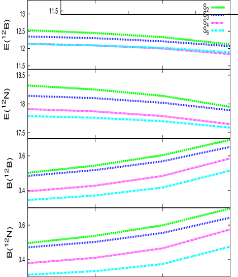
Figure 1: (Color online) ¹²B and ¹²N ground state energies (in units of MeV) and GT $B$-values within the PQRPA for different s.p. spaces, as function of the $pp$-coupling $t$. The experimental values are: $E(^{12}$B$)=13.37$ MeV, and $E(^{12}$N$)=17.33$ MeV  Ajz85 , and $B(^{12}$B$)=0.466$, and $B(^{12}$N$)=0.526$ Al78 .

Figure 2: Exclusive ¹²C($\nu,e^{-})^{12}$N cross-section $\sigma_{e}(E_{\nu},1^{+}_{1})$ (in units of $10^{-42}$ cm²), plotted as a function of the incident neutrino energy $E_{\nu}$. Results for several single-particle spaces $S_{N}$, and $t=0$, within three different energy intervals, are shown. The experimental data in the DAR region are from Ref. Ath97 .

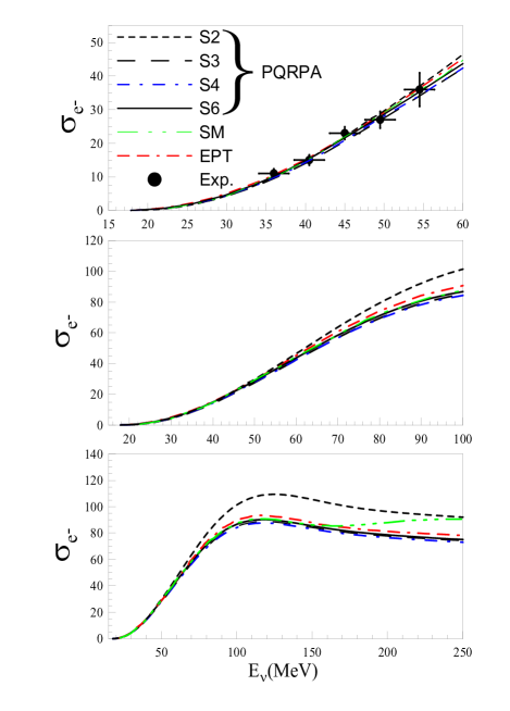
Figure 3: (Color online) Same as in Figure 2, but now $t=0$ for $S_{2}$, and $S_{3}$, $t=0.2$ for $S_{4}$, and $t=0.3$ for $S_{6}$. The SM, and EPT calculations are, respectively, from Refs. Eng96 , and  Fuk88 . The experimental data in the DAR region are from Ref. Ath97 .

III Numerical results and discussion

The major part of the numerical calculations have been done within the PQRPA by employing the $\delta$-interaction (in MeV fm³)

$$V=-4\pi\left(v_{s}P_{s}+v_{t}P_{t}\right)\delta(r),$$

with singlet ($v_{s}$), and triplet ($v_{t}$) coupling constants different for the particle-hole ($ph$), particle-particle ($pp$), and pairing ($pair$) channels Sam08 . This interaction leads to a good description of single and double $\beta$-decays and it has been used extensively in the literature Hir90a ; Krm92 ; Krm93 ; Krm94 . The single-particle wave functions were approximated with those of the HO with the length parameter $b=1.67$ fm, which corresponds to the oscillator energy $\hbar\omega=45A^{-1/3}-25A^{-2/3}$  MeV. The s.p. spaces $S_{2},S_{3},S_{4}$, and $S_{6}$ will be explored.

In Refs. Krm02 ; Krm05 , where the $S_{3}$ space was used, we have pointed out that the values of the coupling strengths $v^{pp}_{s}$, $v^{pair}_{s}$, and $v^{p}_{t}$ used in $N>Z$ nuclei ($v^{pp}_{s}=v^{pair}_{s}$, $v^{pp}_{t}\gtrsim v^{pp}_{s}$), might not be suitable for $N=Z$ nuclei. In fact, the best agreement with data in ¹²C is obtained for: i) the energy of the ground state in ¹²N, $E(^{12}$N), ii) the GT $B$-values in ¹²C, $B(^{12}$N) and $B(^{12}$B), and iii) the exclusive muon capture in ¹²B, $\Lambda^{\rm exc}\equiv\Lambda^{(}1^{+}_{1})$, is obtained when the $pp$ channel is totally switched off, i.e., $v^{pp}_{s}\equiv v^{pp}_{t}=0$. The adopted $ph$ coupling strengths are $v^{ph}_{s}=27$ MeV  fm³ and $v^{ph}_{t}=64$ MeV  fm³ Krm02 . For the $pp$ channel it is convenient to define the parameters

$$s=\frac{v_{s}^{pp}}{v_{s}^{pair}},\hskip 17.07182ptt=\frac{v_{t}^{pp}}{v_{s}^{pair}},$$

where $v_{s}^{pair}=(v_{s}^{pair}(p)+v_{s}^{pair}(n))/2$ Krm94 . As in our previous work on ¹²C, we will use here the same singlet and triplet $pp$ couplings, i.e., $s\equiv t$ Krm02 ; Krm05 . The states with ${\sf J}^{\pi}=0^{+}$, and ${\sf J}^{\pi}=1^{+}$ only depend on $s$, and $t$, respectively, while all remaining depend on both coupling strengths.

The s.p. energies and pairing strengths for $S_{2}$, $S_{3}$, and $S_{4}$ spaces, were varied in a $\chi^{2}$ search to account for the experimental spectra of odd-mass nuclei ¹¹C, ¹¹B, ¹³C, and ¹³N, as explained in Ref. Krm05 . This method, however, is not practical for the space $S_{6}$ which comprises $21$ s.p. levels. Therefore in this case the energies were derived in the way done in Ref. Paa07 , while the pairing strengths were adjusted to reproduce the experimental gaps in ¹²C Sam09 , considering all the quasiparticle energies up to $100$ MeV.

For the purpose of the present study, we also employ the RQRPA theoretical framework  PNVR.04 . In this case the ground state is calculated in the Relativistic Hartree-Bogoliubov model (RHB) using effective Lagrangians with density dependent meson-nucleon couplings and DD-ME2 parameterization LNVR.05 , and pairing correlations are described by the finite range Gogny force BGG.91 . Details of the formalism can be found in Refs. Paa.03 ; PVKC.07 . The RHB equations, and respective equations for mesons are usually solved by expanding the Dirac spinors and the meson fields in a spherical harmonic oscillator basis with $S_{20}$ s.p. space. In the present study of neutrino-nucleus cross sections, with energies of incoming neutrinos up to $600$ MeV, we extend the number of oscillator shells up to $N=30$ in order to accommodate s.p. states at higher energies necessary for description of cross sections involving higher energies of incoming (anti)neutrinos. The number of $2qp$ configurations in the RQRPA is constrained by the maximal excitation energy $E_{2qp}$. Within the RHB+RQRPA framework the oscillator basis is used only in RHB to determine the ground state and single-particle spectra. The resulting wave functions are converted to coordinate space for evaluation of the RQRPA matrix elements. However, it is the original HO basis employed in RHB that determines the maximal $E_{2qp}$ and the size of RQRPA configuration space.

III.1 Weak interaction properties of ¹²N and ¹²B ground states

Let us first compare the QRPA and PQRPA within the smallest configuration space $S_{2}$, which contains $16$ ${\sf J}^{\pi}=1^{+}$ states, and with null $pp$ coupling: $t=0.$ The PQRPA ground state energies in ¹²N, and ¹²B, are, respectively: $\omega_{+1}(1^{+})=18.319$ MeV, and $\omega_{-1}(1^{+})=12.528$ MeV, while the corresponding wave functions read

$$|^{12}{\rm N}\rangle = 0.963|1p^{\pi}_{3/2}1p^{\nu}_{1/2}\rangle+0.232|1p^{\pi}_{3/2}1p^{\nu}_{3/2}\rangle$$ (33)

$$+ 0.122|1p^{\pi}_{1/2}1p^{\nu}_{3/2}\rangle+0.105|1p^{\pi}_{1/2}1p^{\nu}_{1/2}\rangle$$

$$+ \cdots,$$

and

$$|^{12}{\rm B}\rangle = -0.971|1p^{\pi}_{1/2}1p^{\nu}_{3/2}\rangle+0.204|1p^{\pi}_{3/2}1p^{\nu}_{3/2}\rangle$$ (34)

$$- 0.125|1p^{\pi}_{3/2}1p^{\nu}_{1/2}\rangle+0.090|1p^{\pi}_{1/2}1p^{\nu}_{1/2}\rangle$$

$$+ \cdots$$

The analogous QRPA energies are quite similar: $\omega_{+1}(1^{+})=17.992$ MeV, $\omega_{-1}(1^{+})=12.437$ MeV. However, the wave functions are quite different. The main difference is in the fact that QRPA furnishes the same wave functions for all four nuclei ¹²N, ¹⁰B, ¹⁴N, and ¹²B, being that of the ground state:

$$|1^{+}_{GS}\rangle = -0.272|1p^{\pi}_{3/2}1p^{\nu}_{1/2}\rangle-0.759|1p^{\pi}_{3/2}1p^{\nu}_{3/2}\rangle$$ (35)

$$+ 0.356|1p^{\pi}_{1/2}1p^{\nu}_{3/2}\rangle-0.472|1p^{\pi}_{1/2}1p^{\nu}_{1/2}\rangle$$

$$+ \cdots.$$

The difference in the wave functions is an important issue that clearly signalizes towards the need for the number projection. In fact, the PQRPA yields the correct limits ($1p^{\pi}_{3/2}\rightarrow 1p^{\nu}_{1/2}$ and $1p^{\nu}_{3/2}\rightarrow 1p^{\pi}_{1/2}$) for one-particle-one-hole (1p1h) excitations on the ¹²C ground state to reach the ¹²N, and ¹²B nuclei. All remaining configurations in (33), and (34) come from the higher order 2p2h, and 3p3h excitations. Contrary, the QRPA state (35) is dominantly the two-hole excitation $[(1p^{\pi}_{3/2})^{-1},(1p^{\nu}_{3/2})^{-1}]$, which corresponds to the ground state of ¹⁰B. More details on this question can be found in Figure 3 of Ref. Krm05 . The 1p1h amplitudes$[(1p^{\pi}_{3/2})^{-1},1p^{\nu}_{1/2}]$, and $[(1p^{\nu}_{3/2})^{-1},(1p^{\pi}_{1/2})]$ are dominantly present in the following QRPA states

$$|1^{+}_{2}\rangle = 0.708|1p^{\pi}_{1/2}1p^{\nu}_{3/2}\rangle+0.703|1p^{\pi}_{3/2}1p^{\nu}_{1/2}\rangle$$

$$+ \cdots\$$

$$|1^{+}_{4}\rangle = -0.476|1p^{\pi}_{3/2}1p^{\nu}_{1/2}\rangle+0.437|1p^{\pi}_{3/2}1p^{\nu}_{3/2}\rangle$$ (36)

$$+ 0.441|1p^{\pi}_{1/2}1p^{\nu}_{3/2}\rangle-0.096|1p^{\pi}_{1/2}1p^{\nu}_{1/2}\rangle$$

$$+ \cdots$$

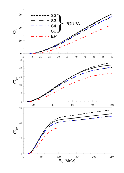
Figure 4: (Color online) The calculated ¹²C(${\tilde{\nu}},e^{+})^{12}$B cross-section $\sigma_{e^{+}}(E_{\tilde{\nu}},1^{+}_{1})$ (in units of $10^{-42}$ cm²), plotted as a function of the incident antineutrino energy $E_{\tilde{\nu}}$. Same as in Figure  3, the value of $t$ is $0$ for the s.p. spaces $S_{2}$, and $S_{3}$, $0.2$ for $S_{4}$ and $0.3$ for $S_{6}$. The EPT calculation from Ref. Fuk88 is also shown.

The wave functions displayed above clearly evidence the superiority of the PQRPA on the QRPA. Therefore from now on only the PQRPA results will be discussed for the exclusive observables.

In Figure  1 we show the ¹²B and ¹²N ground state energies, and the corresponding GT $B$-values within the PQRPA for different s.p. spaces, as function of the $pp$-coupling $t$. One sees that the energies depend rather weakly on both, and agree fairly well with the measured energies: $E(^{12}$B$)=13.37$ MeV, and $E(^{12}$N$)=17.33$ MeV  Ajz85 , although the first one is somewhat underestimated, while the second one is somewhat overestimated. Both GT $B$-values significantly increase with $t$ and diminish when size of the s.p. space is increased. For spaces $S_{2}$ and $S_{3}$ the best overall agreement with data ($B(^{12}$B$)=0.466$, and $B(^{12}$N$)=0.526$ Al78 ) is achieved with $t=0$, while for spaces $S_{4}$ and $S_{6}$ this happens when the couplings are, respectively, $t=0.2$, and $t=0.3$.

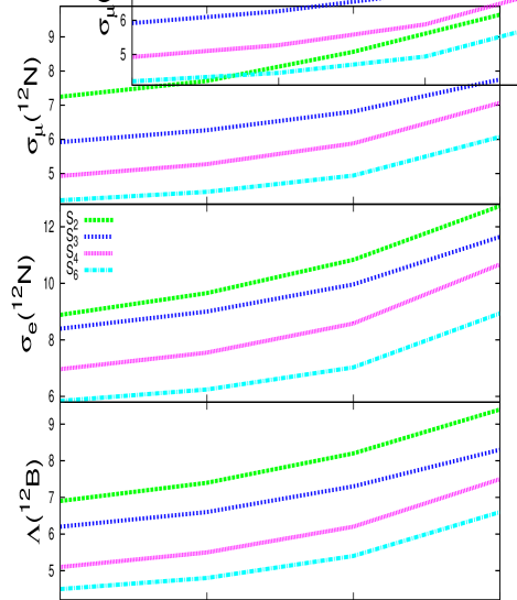
Figure 5: (Color online) Muon capture transition rate to the ¹²B ground state in units of $10^{2}s^{-1}$, and electron and muon folded ECSs to the ¹²N ground state in units of $10^{-42}$ cm² and $10^{-41}$ cm², respectively. The experimental values, in above units, are: $\Lambda(^{12}$B$)=6.2\pm 0.3$ Mil72 , $\overline{\sigma}_{e}(^{12}$N$)=9.1\pm 0.4\pm 0.9$ Ath97 , and $\overline{\sigma}_{e}(^{12}$N$)=8.9\pm 0.3\pm 0.9$ Aue01 , and $\overline{\sigma}_{\mu}(^{12}$N$)=6.6\pm 1.0\pm 1.0$ Ath97a , and $\overline{\sigma}_{\mu}(^{12}$N$)=5.6\pm 0.8\pm 1.0$ Aue02a .

After establishing the PQRPA parametrization, we analyze the behavior of the ECSs of the ground states in ¹²N and ¹²B, as a function of the size of the configuration space. Figure 2 shows the ECSs for the reaction ¹²C($\nu,e^{-})^{12}$N (in units of $10^{-42}$ cm²) for several configuration spaces, and for $t=0$, within three different energy intervals. The top panel represents the DAR region, where experimental data are available Ath97 , and search for neutrino oscillations was done Ath97 ; Zei98 . The middle panel represents the region of interest for supernovae neutrinos, as pointed out in Refs. Aga07 ; Str09 , while the bottom panel shows the asymptotic behavior of the cross-section, which becomes almost constant for $E_{\nu}\simeq 200$ MeV. Within the spaces $S_{2}$ and $S_{3}$ the calculations reproduce quite well the experimental cross sections in the DAR region, as seen from the first panel.

In Figure 3 we show the calculated ECSs for the reaction ¹²C($\nu,e^{-})^{12}$N within several configuration spaces, but now with different values of the $pp$-coupling. From comparison with the experimental data in the DAR region Ath97 one observes that the appropriate values for the coupling $t$ for s.p. spaces $S_{4}$, and $S_{6}$, are, respectively, $t=0.2$, and $t=0.3$, i.e., the same as those required to reproduce the experimental energies and the GR $B$-values in ¹²B, and ¹²N.

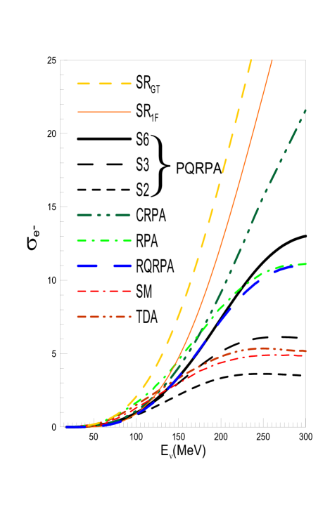
Figure 6: (Color online) Inclusive ¹²C($\nu,e^{-})^{12}$N cross-section $\sigma_{e^{-}}(E_{\nu})$(in units of $10^{-39}$ cm²) plotted as a function of the incident neutrino energy $E_{\nu}$. The PQRPA results within the s.p. spaces $S_{2}$, $S_{3}$, and $S_{6}$, and the same values of $s=t$ as in Figure 3, are compared with two sum rule limits (as explained in the text): $SR_{GT}$, and $SR_{1F}$ obtained with average excitation energy $\overline{{\omega}_{{\sf J}^{\pi}_{n}}}$ of $17.34$, and $42$ MeV, respectively. Several previous RPA-like calculations, namely: RPA Vol00 , CRPA Kol99b , and RQRPA within $S_{20}$ for $E_{2qp}$=100 MeV Paa07 , as well as the SM  Vol00 , and the TDA Con72 are also shown.

This change of parametrization hint at the self-consistency of the PQRPA, and comes from the fact that in this model: i) the GT strength allocated in the ground state is moved to another $1^{+}$ states when the size of the space is increased, and ii) the effect of the $pp$ residual interaction goes in the oppositive direction, returning the GT strength to the $1^{+}_{1}$ state. Only for the space $S_{2}$ the cross-section $\sigma_{e^{-}}(E_{\nu},1^{+}_{1})$ is appreciable larger (at $E_{\nu}\gtrsim 60$ MeV) than for other spaces, which is just because of the small number of configurations in this case. In the same figure are exhibited as well the results for the ECSs evaluated within the SM Eng96 , and the EPT Fuk88 . Both of them agree well with the data and with the present calculation.

The results for the reaction $({\tilde{\nu}},e^{+})$ to the ground state in ¹²B are shown in Figure 4. The cross-section $\sigma_{e^{+}}(E_{\tilde{\nu}},1^{+}_{1})$ is similar to that produced by neutrinos but significantly smaller in magnitude. When compared with the EPT result  Fuk88 , which are also shown in the same figure, one notices that they are considerable different. To some extent this is surprising as in the case of neutrinos the two models yield very similar results. One should remember that in the EPT model the axial form factor, used for both neutrinos and antineutrinos, is gauged to the average of the GR $B$-values in ¹²B, and ¹²N, which, in turn, are well reproduced by the PQRPA. Therefore it is difficult to understand why the EPT results agree with the present calculations for neutrinos and disagree for antineutrinos.

In Figure 5 we show the dependence on the configuration space of the exclusive muon capture transition rate $\Lambda(1^{+}_{1})$ to the ¹²B ground state, and the electron and muon flux-averaged ECSs, given by (31), to the ¹²N ground state, i.e., $\overline{{\sigma}}_{\epsilon}(1^{+}_{1})$, and $\overline{{\sigma}}_{\mu}(1^{+}_{1})$. As in Refs. Krm02 ; Krm05 the electron neutrino distribution $n_{e}(E_{\nu})$ was approximated with the Michel energy spectrum Kol99a ; Arm02 , and for the muon neutrinos we used $n_{\mu}(E_{\nu})$ from Ref. LSND . The energy integration is carried out in the DAR interval $m_{e}+{\omega}_{J_{f}}\leq\Delta_{J_{f}}^{\rm DAR}\leq 52.8$ MeV for electrons and in the DIF interval $m_{\mu}+{\omega}_{J_{f}}\leq\Delta_{J_{f}}^{\rm DIF}\leq 300$ MeV for muons. From Figure 5, and comparison with experimental data:

$\Lambda(^{12}$B$)=6.2\pm 0.3$ Mil72 ,

$\overline{\sigma}_{e}(^{12}$N$)=9.1\pm 0.4\pm 0.9$ Ath97 , $8.9\pm 0.3\pm 0.9$ Aue01 ,

$\overline{\sigma}_{\mu}(^{12}$N$)=6.6\pm 1.0\pm 1.0$ Ath97a , $5.6\pm 0.8\pm 1.0$ Aue02a ,

one finds out, as for results shown in Figures 1, and 3, the model self-consistency between s.p. spaces and the $pp$-couplings. That is, for larger s.p. spaces larger values of $t$ are required. In brief, the experimental data of $\overline{\sigma}_{e}(^{12}$N), and $\overline{\sigma}_{\mu}(^{12}$N) are well reproduced by the PQRPA. The same is true for the SM calculations Hay00 ; Vol00 , while in RPA, and QRPA models they are strongly overestimated, as can be seen from Table II in Ref. Vol00 , and Table 1 in Ref. Sam06 .

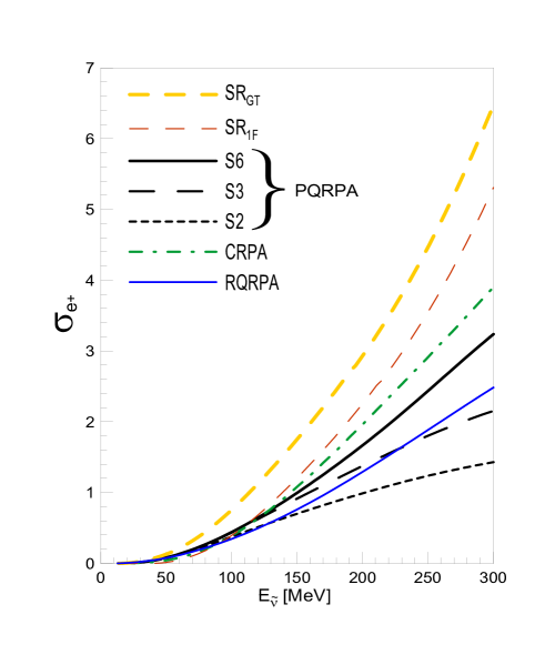
Figure 7: (Color online) Inclusive ¹²C($\tilde{\nu},e^{+})^{12}$B cross-section $\sigma_{e^{+}}(E_{\nu})$ (in units of $10^{-39}$ cm²) plotted as a function of the incident neutrino energy $E_{\tilde{\nu}}$. All results were obtained in the same way as in the neutrino case in Figure 6.

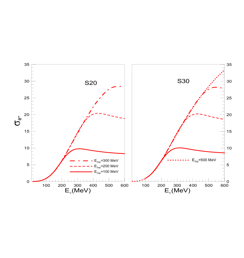
Figure 8: (Color online) Inclusive ¹²C($\nu,e^{-})^{12}$N cross-section $\sigma_{e^{-}}(E_{\nu})$(in units of $10^{-39}$ cm²) plotted as a function of the incident neutrino energy $E_{\nu}$, evaluated in RQRPA with different configuration spaces. These cross sections are plotted as functions of the incident neutrino energy with different cut-off of the $E_{2qp}$ quasiparticle energy as it is explained in the text. The left and right panels show the cross section evaluated with $S_{20}$, and $S_{30}$ s.p. spaces. The last cross section shows that the convergence of the calculation is achieved up to 600 MeV of incident neutrino energy.

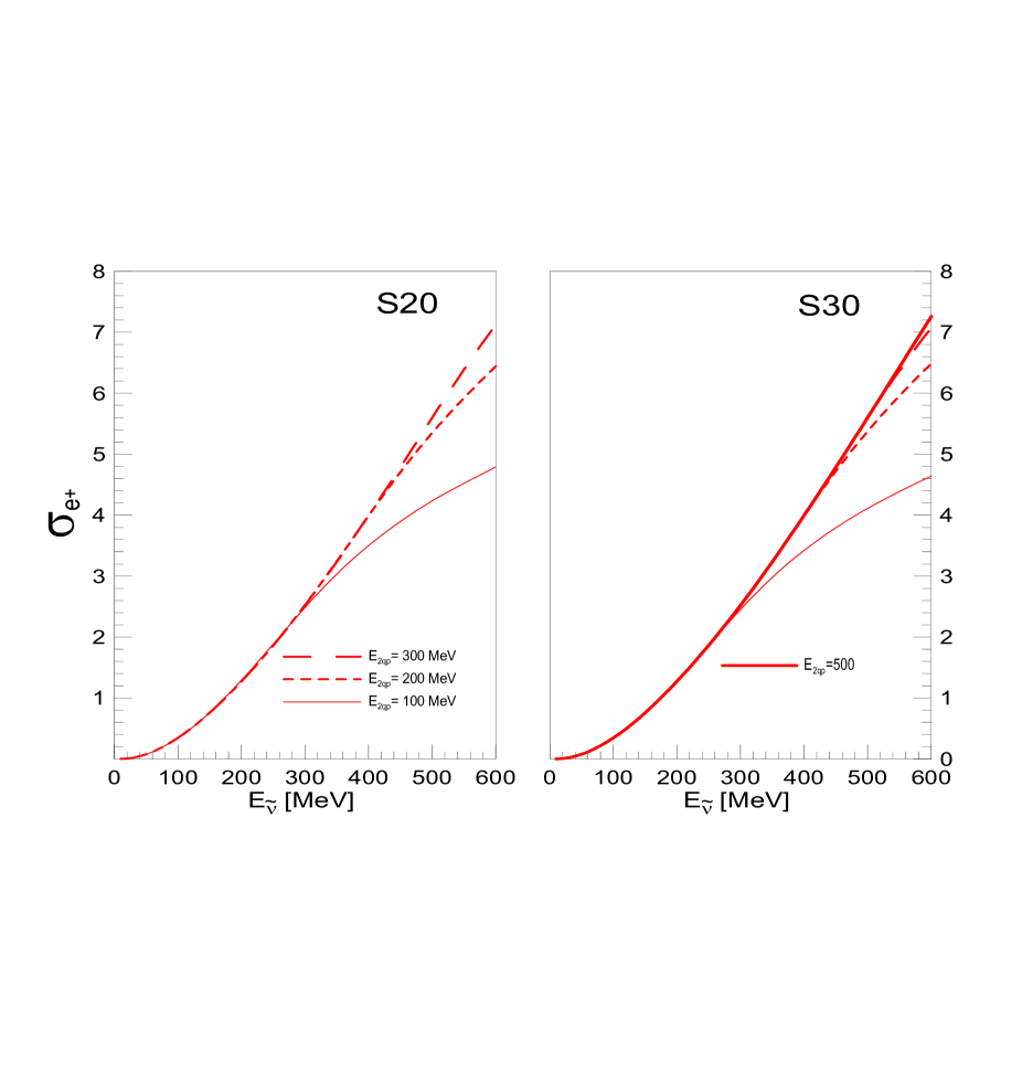
Figure 9: (Color online) Same as in Figure 8 but for the ¹²C($\tilde{\nu},e^{+})^{12}$B cross-section $\sigma_{e^{+}}(E_{\tilde{\nu}})$.

III.2 Inclusive cross-sections ¹²C($\nu,e^{-})^{12}$N and ¹²C($\tilde{\nu},e^{+})^{12}$B, and Sum Rule

In Figure 6 we confront the PQRPA results for the ICS $\sigma_{e^{-}}(E_{\nu})$ within spaces $S_{2}$, $S_{3}$, and $S_{6}$ with the corresponding sum-rules ${\sigma}_{e^{-}}^{SR}(E_{\nu})$ evaluated from (53). One immediately sees that the PQRPA results depend very strongly on the size of the employed s.p. space. On the other hand, as already mentioned in the Appendix B, the sum rule ${\sigma}_{e^{-}}^{SR}(E_{\nu})$ depends on the average energy $\overline{{\omega}_{{\sf J}^{\pi}_{n}}}$. Here we use two values $\overline{{\omega}_{{\sf J}^{\pi}_{n}}}=17.34$ MeV, which is the ground state energy ¹²N, (GT-resonance), and $\overline{{\omega}_{{\sf J}^{\pi}_{n}}}=42$ MeV, which is roughly the energy of the first forbidden resonance Kr83 . The corresponding curves in Figure 6 are labeled, respectively, as $SR_{GT}$, and $SR_{1F}$. They should be the upper limits for allowed and first forbidden transitions, respectively. The validity of these sum rules is questionable for neutrinos energies of several hundred MeV, as already pointed out by Kuramoto et al. Kur90 . In fact, we note that the cross section $SR_{GT}$ ($SR_{1F}$) exceeds the free particle cross section ${\sigma}_{6}\equiv 6{\sigma}(\nu_{e}+n\rightarrow e^{-}+p)$ for $E_{\nu}>200$ MeV ($E_{\nu}>300$ MeV) Bud03 .

Several previous SM and RPA-like calculations of ${\sigma}_{e^{-}}(E_{\nu})$, employing different effective axial-vector coupling constants, and different s.p. spaces, are exhibited in Figure 6 as well, namely:

a) TDA Con72 , with $g_{\scriptscriptstyle A}=1.23$, and $S_{2}$,

b) SM and RPA Vol00 , with $g_{\scriptscriptstyle A}=0.88$, and $S_{3}$,

c) CRPA Kol99b , with $g_{\scriptscriptstyle A}=1.26$, and $S_{4}$,

d) RQRPA Paa07 , with $g_{\scriptscriptstyle A}=1.23$, $S_{20}$, and $E_{2qp}$=100 MeV.

It is important to specify the values $g_{\scriptscriptstyle A}$ because the partial cross sections are predominantly of the axial-vector type (specially the allowed ones), which are proportional to $g_{\scriptscriptstyle A}^{2}$. In spite of very significant differences in $g_{\scriptscriptstyle A}$, and the s.p. spaces, the different calculations of $\sigma_{e^{-}}(E_{\nu})$ yield quite similar results for energies $E_{\nu}\lesssim 130$ MeV, lying basically in vicinity of the the sum-rule result $SR_{1F}$. But for higher energies they could become quite different, and are clearly separated in two groups at $E_{\nu}=300$ MeV. In the first group with ${\sigma}_{e^{-}}(E_{\nu})\lesssim 5\times 10^{-39}$ cm² are: the SM, TDA, and PQRPA within spaces $S_{2}$, $S_{3}$, while in the second one with ${\sigma}_{e^{-}}(E_{\nu})\gtrsim 10\times 10^{-39}$ cm² are: the RPA, RQRPA, CRPA and PQRPA within space $S_{6}$. Volpe et al. Vol00 have found that the difference between their SM and RPA calculations is due to differences in the correlations taken into account, and to a too small SM space. We also note that only the CRPA result approaches the sum rule limits for $E_{\nu}>200$ MeV.

Similar results for the inclusive ¹²C($\tilde{\nu},e^{+})^{12}$B cross-section $\sigma_{e^{+}}(E_{\tilde{\nu}})$ are displayed in Figure 7, and analogous comments can be done here. For the comparison, we show in the figure the antineutrino-¹²C cross-sections evaluated with the CRPA Kol99b .

III.3 Large configuration spaces

As there are no experimental data on flux unfolded ICSs for $E_{\nu}\leq 400$ MeV we cannot conclude which of the results displayed in Figures 6, and 7 are good and which are not. We can only conclude that the ICSs strongly depend on the size of the s.p. space. In the PQRPA calculations we are not able to use spaces lager than $S_{6}$ because of numerical difficulties. Thus instead of using the PQRPA, from now on we employ the RQRPA where such calculations are feasible. It is important to note that within the RHB+RQRPA model the oscillator basis is used only in the RHB calculation in order to determine the ground state and the single-particle spectra. The wave functions employed in RPA equations are obtained by converting the original HO basis to the coordinate representation. Therefore, the size of the RQRPA configuration space and $2qp$  energy cut-offs are determined by the number of oscillator shells in the RHB model.

First, we analyze the effect of the cut-off energy within the $S_{20}$ space on $\sigma_{e^{-}}(E_{\nu})$ for $E_{\nu}$ up to $600$ MeV. From the left panel in Figure 8 one sees that at high energies this cross-section increases roughly by a factor of two when $E_{2qp}$ is augmented from $100$ to $200$ MeV. The increase of the cross-section is also quite important when $E_{2qp}$ is moved from $200$ to $300$ MeV. For the limiting value of $E_{2qp}$=300 MeV, all possible configurations are included in RQRPA calculations. Next, we do the same within the $S_{30}$ space, and the resulting $\sigma_{e^{-}}(E_{\nu})$ are displayed on the right panel of Figure 8. From the comparison of both panels it is easy to figure out that up to $E_{2qp}=300$ MeV the cross sections obtained with the $S_{30}$ space are basically the same to those calculated with the $S_{20}$ space. Small differences between the cross sections using $S_{20}$ and $S_{30}$ spaces for $E_{2qp}$ up to 300 MeV are caused by modifications of positive-energy single-particle states contributing to the QRPA configuration space within the restricted $2qp$ energy window. But, for $E_{\nu}\gtrsim 400$ MeV additional transition strength appears in the $S_{30}$ space when $E_{2qp}$ is moved up to $400$ MeV, from where further increase in $E_{2qp}$ has a very small effect. We conclude therefore that the configuration space engendered by $N=20$ HO shells with $E_{2qp}=300$ MeV, is large enough to describe $\sigma_{e^{-}}(E_{\nu})$ with $E_{\nu}$ up to $400$ MeV. Similarly, the space brought about by $N=30$ HO shells with $E_{2qp}=400$ MeV is appropriate to account for $\sigma_{e^{-}}(E_{\nu})$ up to $E_{\nu}=600$ MeV. For larger neutrino energies very likely we would have to continue increasing the number of shells.

Analogous results for antineutrino ICSs $\sigma_{e^{+}}(E_{\tilde{\nu}})$ are displayed in Figure 9. One notes important differences in comparison with $\sigma_{e^{-}}(E_{\nu})$ shown in Figure 8. First, here the spaces $S_{20}$ and $S_{30}$ yield almost identical results in the entire interval of antineutrino energies up to $E_{\tilde{\nu}}=600$ MeV. Second, the successive increase in the cross-sections when the cut-off $E_{2qp}$ is augmented in steps of $100$ MeV are smaller, and decrease more rapidly than in the neutrino case. This suggests that the configuration space is now sufficiently large to appropriately account for $\sigma_{e^{+}}(E_{\tilde{\nu}})$ even at antineutrino energies larger than $600$ MeV.

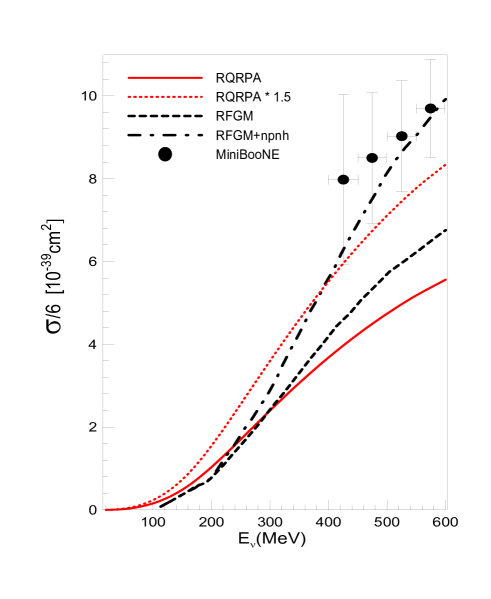
Figure 10: (Color online) The calculated RQRPA (within $S_{30}$ and $E_{2qp}=500$ MeV) quasi-elastic ($\nu_{e},^{12}$C) cross section per neutron (full line) is compared with that for the ($\nu_{\mu},^{12}$C) scattering data measured at MiniBooNE MiniBooNE ; with dotted line is shown the same calculation but renormalized by a factor $1.5$. Also are displayed the calculations done by Martini et al. Mart09 ; Mart10 within the RFGM for pure (1p-1h) excitations (dashed line), and with the inclusion of the np-nh channels (dot-dashed line).

At present, due to numerical difficulties, we cannot perform the RQRPA calculations for the full range of neutrino energies where the QE cross section was measured at MiniBooNE MiniBooNE , but only up to 0.6 GeV. However, we feel that it could still be illustrative for comparison with data. This is done in Figure 10, which is basically a piece of Figure 21 Ref. Mart09 for the QE $\sigma_{\mu^{-}}(E_{\nu})$ (see also Ref. Mart10 ), where is incorporated our result for $\sigma_{e^{-}}(E_{\nu})$ from Figure 8 for $S_{30}$ and $E_{2qp}=500$ MeV. As already pointed out in the Introduction, at relatively high energies ($E_{\nu}>300$ MeV) the electron and muon neutrino cross sections converge to each other, and therefore, in the present analysis, the electron neutrino cross section provides a reasonable upper limit estimate. One sees that we underestimate the data by almost a factor of two. But one should keep in mind that, while we use $g_{\scriptscriptstyle A}=1$ (see (4)) in the RFGM calculation done by Martini et al. Mart09 ; Mart10 $g_{\scriptscriptstyle A}=1.255$ was used. Being the axial-vector contribution dominant for the latter value of the coupling constant, one would have to re-normalize our $\sigma_{e^{-}}(E_{\nu})$ by a factor $\sim 1.5$. Such a result is also shown in Figure  10, and although the resulting cross section still underestimates somewhat the data for $\sigma_{\mu^{-}}(E_{\nu})$, it is notably superior to the pure 1p-1h result from Ref. Mart09 , where good agreement with the data is achieved only after considering additional two-body (2p-2h) and three-body (3p3h) decay channels. One should keep in mind, however, that as the weak decay Hamiltonian is one-body operator, these excitations are only feasible via the ground-state correlations (GSC), which basically redistribute the 1p-1h transition strength without increasing its total magnitude when the initial wave function is properly normalized. In the present work, as well as in all SM-like calculations, the GSC, and a normalized initial state wave function are certainly considered to all orders in perturbation theory through the full diagonalization of the hamiltonian matrix. On the other hand, in Refs. Mart09 ; Mart10 the GSC are taken into account in second order perturbation theory, but there are no references to the normalization of the ¹²C ground-state wave function. How to carry out the normalization in the framework of the infinite nuclear matter model is discussed in a recent paper related to the nonmesonic weak decay of the hypernucleus ${}^{12}_{\Lambda}$C Bau10 ; see also Refs. Ma91 ; Va92 ; Ma95 .

III.4 Multipole decomposition of cross-sections

We did not mention yet the contributions of different multipoles to the ICSs. Normally, the RHB model within $S_{20}$, and with ${\sf J}^{\pi}\leq 7^{\pm}$, provides converged results for RQRPA excitation spectra at incident neutrino energies $E_{\nu}\leq 300$ MeV as seen from Figure 2 in Ref. Paa07 . But this is not the case for neutrino-nucleus cross sections at energies $E_{\nu}\gtrsim 300$ MeV where one has to consider large cutoff energies $E_{2qp}$. In fact, it is necessary to consider more and more multipoles according as the configuration space is enlarged by increasing $E_{2qp}$. This is illustrated in Figure 11 for the case of $E_{2qp}=500$ MeV. One sees that are significant all multipoles up to ${\sf J}^{\pi}=14^{\pm}$ for neutrinos, and up to ${\sf J}^{\pi}=11^{\pm}$ for antineutrinos.

Figure 11: (Color online) Left and right panels show, respectively, the cross sections $\sigma_{e^{-}}(E_{\nu})$, and $\sigma_{e^{+}}(E_{\tilde{\nu}})$ (in units of $10^{-39}$ cm²) evaluated in RQRPA for $S_{20}$, and $S_{30}$ s.p. spaces with the cutoff $E_{2qp}=500$ MeV, and different maximal values of ${\sf J}^{\pm}$, with ${\sf J}$ going from $1$ up to $14$ for neutrinos, and from $1$ up to $11$ for antineutrinos.

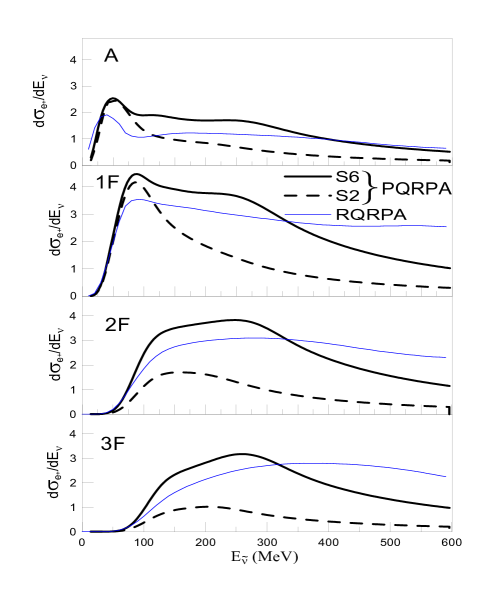
Figure 12: (Color online) Left panel: Allowed ($J^{\pi}=0^{+},1^{+}$), first-forbidden ($J^{\pi}=0^{-},1^{-},2^{-}$), second-forbidden ($J^{\pi}=2^{+},3^{+}$), and third-forbidden ($J^{\pi}=3^{-},4^{-}$) inclusive ¹²C($\tilde{\nu},e^{+})^{12}$B cross-section $\sigma_{e^{+}}(E_{\tilde{\nu}})$ (in units of $10^{-42}$ cm²), plotted as a function of the incident neutrino energy $E_{\tilde{\nu}}$. Right panel: Same as left panel but now for $d\sigma_{e^{+}}(E_{\tilde{\nu}})/dE_{\tilde{\nu}}$ (in units of $10^{-42}$ cm² MeV${}^{-1})$.

Next we discuss the partial multipole contributions to the ICS, having in view the degree of forbiddenness of the transition matrix elements, namely,

$\bullet$ Allowed: $\sigma^{A}_{e^{+}}(E_{\tilde{\nu}})$, with ${\sf J}^{\pi}=0^{+},1^{+}$,

$\bullet$ First-forbidden $\sigma^{1F}_{e^{+}}(E_{\tilde{\nu}})$, with ${\sf J}^{\pi}=0^{-},1^{-},2^{-}$,

$\bullet$ Second-forbidden $\sigma^{2F}_{e^{+}}(E_{\tilde{\nu}})$, with ${\sf J}^{\pi}=2^{+},3^{+}$, and

$\bullet$ Third-forbidden $\sigma^{3F}_{e^{+}}(E_{\tilde{\nu}})$ with ${\sf J}^{\pi}=3^{-},4^{-}$,

cross-sections. Thus, in the left panel of Figure 12 we show these individual contributions for the inclusive ¹²C($\tilde{\nu},e^{+})^{12}$B cross-section $\sigma_{e^{+}}(E_{\tilde{\nu}})$, evaluated within both the PQRPA (spaces $S_{2}$, and $S_{6}$) the RQRPA (space $S_{30}$ with $E_{2qp}=500$ MeV).

The same is done for the corresponding derivatives, i.e., the spectral functions $d\sigma_{e^{+}}(E_{\tilde{\nu}})/dE_{\tilde{\nu}}$, on the right panel of the same figure. Several conclusions can be drawn. First, as in the case of total $\sigma_{e^{+}}(E_{\tilde{\nu}})$, they depend very strongly on the size of the configuration space. This dependence, in turn, increases with the degree of forbiddenness; that is, it is more pronounced for first-forbidden than for allowed transitions, and so on. Second, within the PQRPA the allowed cross-section $\sigma^{A}_{e^{+}}(E_{\tilde{\nu}})$ exhibits a resonant pattern at low energy, and is dominant for $E_{\tilde{\nu}}\lesssim 50$ MeV. For large s.p. spaces its contribution is quite significant even at $E_{\tilde{\nu}}=500$ MeV. In the case of RQRPA, the spectral function $d\sigma^{A}_{e^{+}}(E_{\tilde{\nu}})/dE_{\tilde{\nu}}$ also displays low-energy resonant structure, and $\sigma^{A}_{e^{+}}(E_{\tilde{\nu}})$ is always smaller in magnitude than in the PQRPA case. Third, $\sigma^{1F}_{e^{+}}(E_{\tilde{\nu}})$ is peaked at $E_{\tilde{\nu}}\sim 75$ MeV, and its contribution is always larger than that of $\sigma^{A}_{e^{+}}(E_{\tilde{\nu}})$ for $E_{\tilde{\nu}}\gtrsim 150$ MeV. Fourth, $\sigma^{2F}_{e^{+}}(E_{\tilde{\nu}})$, and $\sigma^{3F}_{e^{+}}(E_{\tilde{\nu}})$ mainly contribute in the interval $150\lesssim E_{\tilde{\nu}}\lesssim 400$ MeV, and their overall contributions are of the same order of magnitude, and comparable to that of the $\sigma^{1F}_{e^{+}}(E_{\tilde{\nu}})$. Fifth, the contributions of the remaining multipoles with ${\sf J}^{\pi}=4^{+},5^{\pm},6^{\pm},7^{\pm}$ are always very small for the space $S_{2}$, but are quite sizeable for $S_{6}$ at high energies. For instance, at $E_{\tilde{\nu}}=100,300,600$ MeV they contribute, respectively with $0.02\%,0.86\%,1.18\%$ within the space $S_{2}$, and $0.04\%,14\%,20\%$ for $S_{6}$. With further increase of the single-particle basis, configurations from higher multipoles become more pronounced at higher neutrino energies. In particular, the sum of contributions coming from ${\sf J}^{\pi}=4^{+},\cdots,11^{\pm}$ multipoles when evaluated within the RQRPA using the space $S_{30}$ and maximal value of $E_{2qp}$=500 MeV, are 1.1%, 14.4%, and 33.2% at $E_{\nu}$=100, 300, and 600 MeV, respectively.

Recently Lazauskas and Volpe Laz07 ; Vol04 have suggested the convenience of performing nuclear structure studies using low energy neutrino and antineutrino beams. Because of feasibility reasons the flux covers $80$ MeV only. Nevertheless, from the analysis of ¹⁶O, ⁵⁶Fe, ¹⁰⁰Mo and ²⁰⁸Pb nuclei within the QRPA using the Skyrme force they were able to disentangle the multipole distributions of forbidden cross-sections, showing that the forbidden multipole contribution is different for various nuclei. In this work we extend this kind of study to ¹²C.

In Table 1 we show the results for the flux-averaged cross sections $\overline{{\sigma}}_{e^{+}}$ for the reaction ${}^{12}{\rm C}({\tilde{\nu}},e^{+})^{12}{\rm B}$. In (32) we have used the same antineutrino fluxes $n_{e^{+}}(E_{\tilde{\nu}})$ as in Ref. Laz07 , i.e., the DAR flux, and those produced by boosted ⁶He ions with different values of time dilation factor $\gamma=1/\sqrt{1-v^{2}/c^{2}}$. Results of two calculations are presented: i) PQRPA within $S_{6}$, and ii) RQRPA within $N=20$, and cutoff $E_{2qp}=300$ MeV. One sees that in both models, and principally in the PQRPA, the allowed transitions dominate the forbidden one, and specially for the low-energy beam with $\gamma=6$. The contributions of the second-forbidden processes are very small in all the cases, while those coming from third-forbidden ones are always negligible. All this is totally consistent with the results shown in Figure 12, from where it is clear that to study second and third forbidden reactions in ¹²C, one would need fluxes $n_{e^{+}}(E_{\tilde{\nu}})$ with $E_{\tilde{\nu}}$ at least up to $\gtrsim 150$ MeV. It should also be stressed that our results both for allowed and forbidden transitions fully agree with those obtained in Ref. Laz07 ; the difference in ¹⁶O comes from the double-shell closure in this nucleus.

Table 1:  Fraction (in %) of flux-averaged cross sections $\overline{{\sigma}}_{e^{+}}$ for ${}^{12}{\rm C}({\tilde{\nu}},e^{+})^{12}{\rm B}$ for allowed (A), first-forbidden (1F), second-forbidden (2F), and third-forbidden (3F) processes. The antineutrino fluxes $n_{e^{+}}(E_{\tilde{\nu}})$ are the same as in Ref. Laz07 , i.e., the DAR flux, and those produced by boosted ⁶He ions with different values of $\gamma=1/\sqrt{1-v^{2}/c^{2}}$. Results of two calculations are presented: i) PQRPA within $S_{5}$, and ii) RQRPA within $N=30$, and cutoff $E_{2qp}=300$ MeV.

	DAR	$\gamma$
		6	10	14
A
PQRPA	79.43	92.09	77.00	63.01
RQRPA	84.40	94.88	82.25	67.15
1F
PQRPA	20.03	7.83	22.16	33.76
RQRPA	15.10	4.13	16.86	29.61
2F
PQRPA	0.51	0.07	0.78	2.89
RQRPA	0.55	0.08	0.81	2.91
3F
PQRPA	0.018	0.002	0.04	0.33
RQRPA	0.025	0.011	0.05	0.33

III.5 Supernova neutrinos

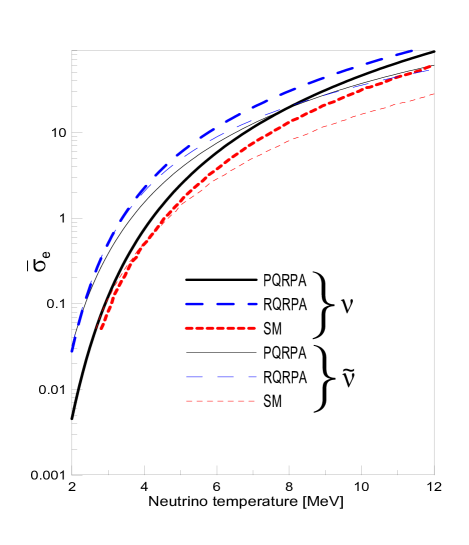
Figure 13: (Color online) Flux-averaged neutrino and antineutrino cross sections $\overline{{\sigma}}_{e^{\pm}}$ in ¹²C with typical supernovae fluxes.

We also address briefly the $\nu/\tilde{\nu}$-¹²C nucleus cross-sections related with astrophysical applications, the knowledge of which could have important implications. For this purpose, are evaluated the $\overline{{\sigma}}_{e^{\pm}}$ folded with supernovae $\nu/\tilde{\nu}$ spectra represented by a normalized Fermi-Dirac distribution with temperatures in the interval $T_{\nu_{e}}=2-12$ MeV, which includes the most commonly used values are $T_{\nu_{e}}=3.2$ MeV and $T_{\bar{\nu}_{e}}=5.0$ MeV. For mean energies $\langle E_{\nu}\rangle\approx 3.15\times T_{\nu}$, and zero chemical potential Woo90 ; Kei03 the neutrino flux is

$$n_{e}(E_{\nu})=\frac{0.5546}{T_{\nu}^{3}}\frac{E_{\nu}^{2}}{e^{E_{\nu}/T_{\nu}}+1},$$ (37)

and similarly for antineutrinos. For the sake of simplicity we do not analyze same relevant aspects of $n_{e}(E_{\nu})$ in supernova simulation, such as the MSW effect (see, for example, Ref. Akh00 ), and the spectral swapping of the neutrino flux (Ref. Dun07 ). In Figure 13 we confront the $\nu-^{12}$C cross sections averaged over supernova $\nu$-fluxes for the range of $T_{\nu}=2-12$ MeV, obtained within following calculations:

i) PQRPA within $S_{6}$,

ii) RQRPA within $S_{30}$ and $E_{2qp}=500$ MeV, and

iii) SM done by Suzuki et al. Suz06 with the SFO Hamiltonian (the PSDMK2 interaction yields a quite similar result).

As seen from Figure 13, in the vicinity of the temperatures mentioned at the beginning ($T_{\nu}=3-5$ MeV), these three calculations yield, respectively, that: i) $\overline{{\sigma}}_{e^{+}}$ is significantly larger than $\overline{{\sigma}}_{e^{-}}$, ii) $\overline{{\sigma}}_{e^{-}}$ is only slightly larger than $\overline{{\sigma}}_{e^{+}}$, and iii) $\overline{{\sigma}}_{e^{+}}\cong\overline{{\sigma}}_{e^{-}}$. Both SM cross sections are always smaller than those obtained in the the other two calculations, and specially in comparison with the RQRPA one.

IV Summary and concluding remarks

The present work is a continuation of our previous works Krm02 ; Krm05 . In fact, the formalism for weak interaction processes introduced there is now elaborated more thoroughly yielding very simple expressions for the transition rates, which greatly facilitate the numerical calculation. This is done through the separation of the nuclear matrix elements into their real and imaginary parts, which, in turn, permits to split the transition rates, for neutrino-nucleus reactions (II) into natural (43) and unnatural parity (44) operators. Similar separation is done for the muon capture transition rate (64) in Eqs. (65) and (66). Moreover, consequences of explicit violation of CVC hypothesis by the Coulomb field (21) are addressed for the first time, and the sum rule approach for the inclusive cross section, proper to the present formalism, has been worked out in the Appendix B. For the sake of completeness, the extreme relativistic limit of neutrino-nucleus cross section is also presented in the Appendix C, where in the formula for transition rates turn out to be still simpler. We note that, except at very low neutrino energies, they can be used without any restriction in practical applications.

We have discussed in details the inclusive properties that comprise:

i) Ground state energies in ¹²B and ¹²N, and the corresponding GT $B$-values (Figure  1),

ii) Exclusive ¹²C($\nu,e^{-})^{12}$N cross-section $\sigma_{e}(E_{\nu},1^{+}_{1})$, as a function of the incident neutrino energy $E_{\nu}$ (Figures 2, and  3),

iii) Exclusive ¹²C(${\tilde{\nu}},e^{+})^{12}$B cross-section $\sigma_{e^{+}}(E_{\tilde{\nu}},1^{+}_{1})$, as a function of the incident antineutrino energy $E_{\tilde{\nu}}$ (Figure  4), and

iv) Muon capture transition rate to the ¹²B ground state, and electron and muon folded cross-sections to the ¹²N ground state $\overline{{\sigma}}_{\epsilon}(1^{+}_{1})$, and $\overline{{\sigma}}_{\mu}(1^{+}_{1})$ (Figure  5).

Special attention was paid to the interplay between the size of the configuration space, and the magnitude of the residual interaction within the $pp$-channel. It was found that as the first becomes larger, the second has to increase to obtain the agreement with the experimental data for the exclusive observables.

The main purpose of our discussion of exclusive properties was to put in evidence the limitations of the RPA and the QRPA models. The basic problem in the implementation of the RPA is the lack of pairing correlations, i.e. the inability for opening the $1p_{3/2}$ shell, while deficiency of the standard QRPA is in the non-conservation of the number of particles, as evidenced by the wave functions (33), (34), and (35) presented in Sec. III. In this way we have definitively established that the SM and the PQRPA are proper theoretical frameworks to describe the ground state properties of ¹²B and ¹²N.

The inclusive cross-sections ¹²C($\nu,e^{-})^{12}$N and ¹²C($\tilde{\nu},e^{+})^{12}$B have been studied within the PQRPA in the same manner as the exclusive ones for $E_{\nu_{e}}$ up to $300$ MeV. As there are no experimental available in this case the comparison is done with the previous calculations only , and displayed in Figures 6, and 7. Here, unlike within Figures 2, 3, and 4, we also show the results obtained with the other RPA-like models  Con72 ; Vol00 ; Kol99b ; Paa07 , which could be a suitable framework for describing global nuclear properties such as it is the inclusive cross-sections.

When the size of the configuration space is enlarged the calculated PQRPA cross-sections, at difference with the exclusive ones, steadily increase, and particulary for neutrino energies larger than $200$ MeV, in spite of including the particle-particle interaction. At low energy they approach to the cross section of the first-forbidden sum-rule limit, but are significantly smaller at high energies both for neutrino and antineutrino.

The largest space that we can deal within the number projection procedure is the one that includes all the orbitals until the $N=6$ HO shell. This is the reason why we have recurred to the RQRPA where it is possible to employ larger configuration spaces. It seems that when the number of shells is increased to $N={30}$, and the cut-off energy $E_{2qp}$ is large enough, the cross sections very likely converge as shown in Figures 8, 9, 10, and 11.

The Figure 10 also indicates that the RQRPA is a promising nuclear model to reproduce the quasi elastic ($\nu_{\mu},^{12}$C) cross section in the region of $E_{\nu_{\mu}}\sim 1$ GeV which has been measured recently at MiniBooNE MiniBooNE . We do not know whether the discrepancy between the experiment and the theory comes from the non completeness of the configuration space or from the smallness of the effective axial-vector coupling constant that we are using $g_{\mbox{\tiny A}}=1$. It could also happens that we need $g_{\mbox{\tiny A}}=1$ for the low energy exclusive cross section and $g_{\mbox{\tiny A}}=1.255$ for the high energy inclusive cross section. We do not understand the reason for such a energy dependence of $g_{\mbox{\tiny A}}$, but it is consistent with the Eq. (23) in Ref. Na82 where it is shown that for the low energy $\beta$-decay $g_{\mbox{\tiny A}}$ could be much more quenched that the total GT strength. We hope to be able to say more on this matter in the next future.

We have also addressed the issue of multipole composition of the inclusive cross sections, by separating them into allowed ($J^{\pi}=0^{+},1^{+}$), first-forbidden ($J^{\pi}=0^{-},1^{-},2^{-}$), second-forbidden ($J^{\pi}=2^{+},3^{+}$), and third-forbidden ($J^{\pi}=3^{-},4^{-}$) processes. The results for the antineutrino reaction ¹²C($\tilde{\nu},e^{+})^{12}$B are displayed in Figure 12 both for the PQRPA and the RQRPA. Of course, similar results are obtained also for neutrinos. We remark that the spectral functions $d\sigma^{A}_{e^{+}}(E_{\tilde{\nu}})/dE_{\tilde{\nu}}$, when evaluated within the PQRPA, clearly put into evidence the resonant structure of the allowed cross-section, which is mainly of the GT type.

The study of the partial ICSs has been related with the proposal done in Refs. Laz07 ; Vol04 of performing nuclear structure studies of forbidden processes by using low energy neutrino and antineutrino beams. From the results shown in Table 1 for the flux-averaged cross sections $\overline{{\sigma}}_{e^{+}}$ in the reaction ${}^{12}{\rm C}({\tilde{\nu}},e^{+})^{12}{\rm B}$ we show that the contribution of allowed transitions decreases gradually in favor of the first forbidden transitions according with the increase of $\gamma$-boost. We conclude that to study high forbidden reactions one would need ${\tilde{\nu}}$-fluxes with $E_{\tilde{\nu}}$ up to $\gtrsim 150$ MeV in ${}^{12}C$.

At the end we considered possible astrophysical applications of the $\nu/\tilde{\nu}$-¹²C nucleus folded cross sections $\overline{{\sigma}}_{e^{\pm}}$, using supernovae $\nu/\tilde{\nu}$ spectra represented by a normalized Fermi-Dirac distribution with mean energy $\langle E_{\nu}\rangle\approx 3.15\times T_{\nu}$, and zero chemical potential. It is found that for temperature $T_{\nu}=3-5$ MeV both the PQRPA and RQRPA models yield significantly larger cross sections that the previously used shell model.

Appendix A Contributions to ${{\cal T}}_{{\sf J}^{\pi}_{n}}({\kappa})$ of natural and unnatural parity states

The real and imaginary parts of the operators ${\sf O}_{{{\alpha}}{\sf J}}$ given by (15) and (23) do not contribute simultaneously. In fact, the $\Re{\sf O}_{{{\alpha}}{\sf J}}$ ($\Im{\sf O}_{{{\alpha}}{\sf J}}$) contributes to natural (unnatural) parity states, which means that we always can work only with real operators, which greatly simplifies the calculations. To see this we note that, while the operators ${{\cal M}}^{\scriptscriptstyle V}_{\sf J}$, ${{\cal M}}^{\scriptscriptstyle A}_{\sf J}$, and

$${{{\cal M}}}^{\scriptscriptstyle A}_{0{\sf J}} = \sum_{{\sf L}={\sf J}\pm 1}(-)^{({\sf J-L}-1)/2}\ F_{{{\sf LJ}0}}j_{\sf L}(\rho)\left[Y_{{\sf L}}(\hat{{\bf r}})\otimes{\mbox{\boldmath$\sigma$}}\right]_{{\sf J}},$$

(38)

are real, ${{\cal M}}^{\scriptscriptstyle A}_{\pm 1{\sf J}}$ and ${{\cal M}}^{\scriptscriptstyle V}_{\pm 1{\sf J}}$ are not. Explicitly,

$${{\cal M}}_{\pm 1{\sf J}}^{\scriptscriptstyle A} = {{\cal M}}_{\pm 1\sf J}^{\scriptscriptstyle A,R}+i{{\cal M}}_{\pm 1\sf J}^{\scriptscriptstyle A,I}$$

$${{\cal M}}_{\pm 1{\sf J}}^{\scriptscriptstyle V} = {{\cal M}}_{\pm 1\sf J}^{\scriptscriptstyle V,R}+i{{\cal M}}_{\pm 1\sf J}^{\scriptscriptstyle V,I}$$ (39)

where

$${{\cal M}}^{\scriptscriptstyle A,R}_{1\sf J} \equiv {{\cal M}}^{\scriptscriptstyle A,R}_{-1\sf J}$$

$$= \sum_{{\sf L}={\sf J}\pm 1}(-)^{({\sf J-L}-1)/2}\ F_{{{\sf LJ}1}}j_{\sf L}(\rho)\left[Y_{{\sf L}}(\hat{{\bf r}})\otimes{\mbox{\boldmath$\sigma$}}\right]_{{\sf J}},$$

$${{\cal M}}^{\scriptscriptstyle A,I}_{1{\sf J}} \equiv -{{\cal M}}^{\scriptscriptstyle A,I}_{-1{\sf J}}=-F_{1{\sf JJ}}j_{\sf J}(\rho)\left[Y_{{\sf J}}(\hat{{\bf r}})\otimes{\mbox{\boldmath$\sigma$}}\right]_{{\sf J}},$$

$${{\cal M}}^{\scriptscriptstyle V,R}_{1\sf J} \equiv {{\cal M}}^{\scriptscriptstyle V,R}_{-1\sf J}$$

$$= \sum_{{\sf L}={\sf J}\pm 1}(-)^{({\sf J-L}-1)/2}\ F_{{{\sf LJ}1}}j_{\sf L}(\rho)\left[Y_{{\sf L}}(\hat{{\bf r}})\otimes{\mbox{\boldmath$\nabla$}}\right]_{{\sf J}},$$

$${{\cal M}}^{\scriptscriptstyle V,I}_{1{\sf J}} \equiv -{{\cal M}}^{\scriptscriptstyle V,I}_{-1{\sf J}}=-F_{1{\sf JJ}}j_{\sf J}(\rho)\left[Y_{{\sf J}}(\hat{{\bf r}})\otimes{\mbox{\boldmath$\nabla$}}\right]_{{\sf J}},$$ (40)

with ${\sf L}\geq 0$, and ${\sf J}\neq 0$. Thus

$${\sf O}_{\pm 1{\sf J}} = i(-g_{\mbox{\tiny A}}\pm\overline{g}_{\mbox{\tiny W}})({{\cal M}}^{\scriptscriptstyle A,R}_{1\sf J}\pm i{{{\cal M}}}^{\scriptscriptstyle A,I}_{1{\sf J}})$$ (41)

$$+ g_{\scriptscriptstyle{V}}({{\cal M}}^{\scriptscriptstyle V,R}_{1\sf J}\pm i{{{\cal M}}}^{\scriptscriptstyle V,I}_{1{\sf J}}),$$

and writing

$${\sf O}_{\emptyset{\sf J}} = {\sf O}_{\emptyset{\sf J}}^{\scriptscriptstyle R}+i{\sf O}_{\emptyset{\sf J}}^{\scriptscriptstyle I},$$

$${\sf O}_{m{\sf J}} = {\sf O}_{m{\sf J}}^{\scriptscriptstyle R}+i{\sf O}_{m{\sf J}}^{\scriptscriptstyle I},$$ (42)

it is not difficult to discover that:

• For natural parity states , with $\pi=(-)^{J}$, i.e., $J^{\pi}=0^{+},1^{-},2^{+},3^{-},\cdots$:

  $${\sf O}_{\emptyset{\sf J}}^{\scriptscriptstyle R} = g_{{\scriptscriptstyle{V}}}{{\cal M}}_{\sf J}^{\scriptscriptstyle V},$$

  $${\sf O}_{{0}{\sf J}}^{\scriptscriptstyle R} = \frac{{\tilde{k}}_{\emptyset}}{{\kappa}}g_{\mbox{\tiny V}}{{\cal M}}_{\sf J}^{\scriptscriptstyle V},$$

  $${\sf O}_{\pm 1{\sf J}}^{\scriptscriptstyle R} = (\pm g_{\mbox{\tiny A}}-\overline{g}_{\mbox{\tiny W}}){{{\cal M}}}^{\scriptscriptstyle A,I}_{1{\sf J}}+g_{\scriptscriptstyle{V}}{{\cal M}}^{\scriptscriptstyle V,R}_{1\sf J},$$ (43)

• For unnatural parity states, with $\pi=(-)^{J+1}$, i.e., $J^{\pi}=0^{-},1^{+},2^{-},3^{+},\cdots$:

  $${\sf O}_{\emptyset{\sf J}}^{\scriptscriptstyle I} = -g_{\scriptscriptstyle{A}}{{\cal M}}^{\scriptscriptstyle A}_{\sf J}-(\overline{g}_{\mbox{\tiny A}}+\overline{g}_{\mbox{\tiny P1}}){{\cal M}}^{\scriptscriptstyle A}_{0{\sf J}},$$

  $${\sf O}_{{0}{\sf J}}^{\scriptscriptstyle I} = (g_{\mbox{\tiny A}}-\overline{g}_{\mbox{\tiny P2}}){{\cal M}}^{\scriptscriptstyle A}_{{0\sf J}},$$

  $${\sf O}_{\pm 1{\sf J}}^{\scriptscriptstyle I} = (g_{\mbox{\tiny A}}\mp\overline{g}_{\mbox{\tiny W}}){{\cal M}}^{\scriptscriptstyle A,R}_{1\sf J}\mp g_{\mbox{\tiny V}}{{{\cal M}}}^{\scriptscriptstyle V,I}_{1{\sf J}}.$$ (44)

These operators have to be used in (II), instead of those defined in (15), and (23).

The correspondence between the individual matrix elements, defined by Donnelly, and Peccei in Eq (3.31)of Ref. Don79 , and the ones used here, is:

$$M_{\sf J} \rightarrow {{\cal M}}^{\scriptscriptstyle V}_{\sf J},$$

$$\Delta_{\sf J} \rightarrow \sqrt{2}{{{\cal M}}}^{\scriptscriptstyle V,I}_{1{\sf J}},$$

$$\Delta^{\prime}_{\sf J} \rightarrow -\sqrt{2}{{{\cal M}}}^{\scriptscriptstyle V,R}_{1{\sf J}},$$

$$\Sigma_{\sf J} \rightarrow \sqrt{2}{{{\cal M}}}^{\scriptscriptstyle A,I}_{1{\sf J}},$$ (45)

$$\Sigma^{\prime}_{\sf J} \rightarrow -\sqrt{2}{{{\cal M}}}^{\scriptscriptstyle A,R}_{1{\sf J}},$$

$$\Sigma_{\sf J}" \rightarrow {{{\cal M}}}^{\scriptscriptstyle A}_{0{\sf J}},$$

$$\Omega_{\sf J} \rightarrow {{{\cal M}}}^{\scriptscriptstyle A}_{{\sf J}}.$$

Moreover, the correspondence between the linear combinations of these matrix elements defined in (Don79, , Eqs. (3.32)) (for ${\hat{L}}_{\sf J}$ see  (Hax79, , Eq. (14))), and the ones introduced here is:

• For natural parity states :

  $${\hat{M}}_{\sf J} = {\sf O}_{\emptyset{\sf J}},$$

  $${\hat{L}}_{\sf J} = {\sf O}_{0{\sf J}},$$

  $${\hat{T}}_{\sf J}^{\rm el}\pm{\hat{T}}_{\sf J}^{\rm mag5} = -\sqrt{2}{\sf O}_{\pm 1{\sf J}},$$ (46)

• For unnatural parity states:

  $${\hat{M}}_{\sf J}^{5} = {\sf O}_{\emptyset{\sf J}},$$

  $$-i{\hat{L}}_{\sf J}^{5} = {\sf O}_{0{\sf J}},$$

  $$i({\hat{T}}_{\sf J}^{\rm el5}\pm{\hat{T}}_{\sf J}^{\rm mag}) = \sqrt{2}{\sf O}_{\pm 1{\sf J}}.$$ (47)

The following relation can also be useful:

$${\sf O}_{\emptyset{\sf J}} = {\hat{{\cal M}}}_{\sf J},$$ (48)

$${\sf O}_{m\sf J} = \left\{\begin{array}[]{ccc}{\hat{{\cal L}}}_{\sf J},&\mbox{for}&m=0\\ -{1\over\sqrt{2}}\left[m{\hat{{{\cal T}}}^{\rm mag}}_{\sf J}+{\hat{{\cal T}}^{\rm el}}_{\sf J}\right],&\mbox{for}&m=\pm 1\end{array}\right.,$$ (51)

where ${\hat{{\cal M}}}_{\sf J}={\hat{M}}_{\sf J}+{\hat{M}}_{\sf J}^{5}$, ${\hat{{\cal L}}}_{\sf J}={\hat{L}}_{\sf J}+{\hat{L}}_{\sf J}^{5}$, ${\hat{{\cal T}}^{\rm el}}_{\sf J}={\hat{T}}_{\sf J}^{\rm el}+{\hat{T}}_{\sf J}^{\rm el5}$, and ${\hat{{\cal T}}^{\rm mag}}_{\sf J}={\hat{T}}_{\sf J}^{\rm mag}+{\hat{T}}_{\sf J}^{\rm mag5}$.

The matrix elements of Kuramoto et al. Kur90 are related with our non-relativistic operators (17) as:

$$|\langle f|{\hat{1}}|i\rangle|^{2} = 4\pi\sum_{{\sf J}^{\pi}_{n}}|\langle{\sf J}^{\pi}_{n}||{{\cal M}}^{\scriptscriptstyle V}_{\sf J}||0^{+}\rangle|^{2},$$

$$|\langle f|{\hat{\sigma}}|i\rangle|^{2} = 4\pi\sum_{{\sf J}^{\pi}_{n}}\sum_{m=0,\pm 1}|\langle{\sf J}^{\pi}_{n}||{{\cal M}}^{\scriptscriptstyle A}_{{m\sf J}}||0^{+}\rangle|^{2},$$

$$\Lambda = \frac{4\pi}{3}\sum_{{\sf J}^{\pi}_{n}}\left[|\langle{\sf J}^{\pi}_{n}||{{\cal M}}^{\scriptscriptstyle A}_{{0\sf J}}||0^{+}\rangle|^{2}\right.$$ (52)

$$- \left.|\langle{\sf J}^{\pi}_{n}||{{\cal M}}^{\scriptscriptstyle A}_{{1\sf J}}||0^{+}\rangle|^{2}\right].$$

In Ref. Kur90 are neglected the relativistic operators ${{\cal M}}^{\scriptscriptstyle A}_{\sf J}$, and ${{\cal M}}^{\scriptscriptstyle V}_{{m\sf J}}$ defined in (LABEL:2.15).

Appendix B Sum Rule Approach

We follow here the sum-rule approach developed by Kuramoto et al. Kur90 , and adapt it to our formalism. We start from Eqs. (LABEL:2.25), and (30), and as in this work we assume that the ${\omega}_{{\sf J}^{\pi}_{n}}$ dependence of the integrand can be ignored, fixing it at a representative value $\overline{{\omega}_{{\sf J}^{\pi}_{n}}}$ . The summation over final nuclear states ${\sf J}^{\pi}_{n}$ then can be carried out by closure, and the ICS is

$${\sigma}_{\ell}^{SR}(E_{\nu}) = G^{2}\frac{|{\bf p}_{\ell}|E_{\ell}}{2\pi}F(Z+S,E_{\ell})$$ (53)

$$\times \int_{-1}^{1}d(\cos\theta){{\cal T}}^{SR},$$

where the lepton energy is $E_{\ell}=E_{\nu}-\overline{{\omega}_{{\sf J}^{\pi}_{n}}}$, while the sum-rule matrix element reads:

$${{\cal T}}^{SR} = \sum_{{\alpha}=\emptyset,0,\pm 1}\langle 0^{+}|O_{\alpha}^{\dagger}O_{\alpha}|0^{+}\rangle{{\cal L}}_{{\alpha}}$$ (54)

$$- 2\Re\left(\langle 0^{+}|O_{\emptyset}^{\dagger}O_{0}|0^{+}\rangle{{\cal L}}_{\emptyset 0}\right).$$

The operators $O_{\alpha}$ are given by (6), and the lepton traces by (Krm05, , Eq. (2.24)). The matrix elements in (54) are proportional to $N(1-D)$, where $N_{N}$ is the number of neutrons (protons), contained in the target nucleus for the neutrino (anti-neutrino) reaction. The correlation functions $D$ come from the Pauli-exclusion-effect, and depend on the type of the operator. One gets:

$${{\cal T}}^{SR} = N_{N}\left(T_{\emptyset}{{\cal L}}_{\emptyset}+\sum_{M}T_{M}{{\cal L}}_{M}-2T_{\emptyset 0}{{\cal L}}_{\emptyset 0}\right),$$ (55)

with

$$T_{\emptyset} \equiv g_{\mbox{\tiny V}}^{2}(1-D_{S})+(\overline{g}_{\mbox{\tiny A}}+\overline{g}_{\mbox{\tiny P1}})^{2}(1-D_{L}),$$

$$T_{0} \equiv \overline{g}_{\mbox{\tiny V}}^{2}(1-D_{S})+(g_{\mbox{\tiny A}}-\overline{g}_{\mbox{\tiny P2}})^{2}(1-D_{L}),$$

$$T_{1} \equiv (g_{\mbox{\tiny A}}-\overline{g}_{\mbox{\tiny W}})^{2}(1-D_{T}),$$ (56)

$$T_{-1} \equiv (g_{\mbox{\tiny A}}+\overline{g}_{\mbox{\tiny W}})^{2}(1-D_{T}),$$

$$T_{\emptyset 0} \equiv -g_{\mbox{\tiny V}}\overline{g}_{\mbox{\tiny V}}(1-D_{S})+(\overline{g}_{\mbox{\tiny A}}+\overline{g}_{\mbox{\tiny P1}})(g_{\mbox{\tiny A}}-\overline{g}_{\mbox{\tiny P2}})(1-D_{L}).$$

The correlation functions $D_{S},D_{L}$ and $D_{S}$ were taken from the SM calculation done by Bell, and Llewellyn Smith Bel71 with HO wave functions, and representing the nuclear ground state by a single determinant wave function. The results for ¹²C are  (Bel71, , Table 1)):

$$D_{S} = e^{-\eta}\left[1+0.148\eta^{2}\right],$$

$$D_{T} = e^{-\eta}\left[0.704+0.148\eta+0.148\eta^{2}\right],$$

$$D_{L} = e^{-\eta}\left[0.704+0.296\eta+0.148\eta^{2}\right],$$ (57)

where $\eta=\frac{1}{2}b^{2}{\kappa}^{2}\cong 0.0558$.

As seen from (29), the factor $|{\bf p}_{\ell}|E_{\ell}$ in (53) behaves as $(E_{\nu}-\overline{{\omega}_{{\sf J}^{\pi}_{n}}})^{2}$, and therefore ${\sigma}_{\ell}^{SR}(E_{\nu})$ depends very critically on the average value for the excitation energy $\overline{{\omega}_{{\sf J}^{\pi}_{n}}}$.

$$E_{\ell} = E_{\nu}-{\omega}_{{\sf J}^{\pi}_{n}},~{}|{\bf p}_{\ell}|=\sqrt{(E_{\nu}-{\omega}_{{\sf J}^{\pi}_{n}})^{2}-m_{\ell}^{2}},$$

$$\kappa = |{\bf p}_{\ell}-{\bf q}_{\nu}|$$ (58)

$$= \sqrt{2E_{\nu}(E_{\ell}-|{\bf p}_{\ell}|\cos\theta)-m_{\ell}^{2}+{\omega}_{{\sf J}^{\pi}_{n}}^{2}},$$

Appendix C Extreme Relativistic Limit

Using the present formalism the ERL, defined by the limit of the lepton velocity $|{\bf p}_{\ell}|/E_{\ell}\rightarrow 1$, yields

$${\sigma}^{ERL}_{\ell}(E_{\nu}) = \sum_{J^{\pi}_{n}}\frac{E^{2}_{\ell}}{2\pi}F(Z+S,E_{\ell})\int_{-1}^{1}d(\cos\theta){{\cal T}}^{ERL}_{{\sf J}^{\pi}_{n}}(\kappa),$$

with

$$\kappa = \sqrt{2E_{\nu}E_{\ell}(1-\cos\theta)+{\omega}_{{\sf J}^{\pi}_{n}}^{2}},$$ (60)

and

$${{\cal T}}^{ERL}_{{\sf J}^{\pi}_{n}}({\kappa}) = {4\pi G^{2}}\left[2\cos^{2}\frac{\theta}{2}\left|\langle{\sf J}^{\pi}_{n}||{\sf O}_{\emptyset{{\sf J}}}({\kappa})-\frac{k_{\emptyset}}{{\kappa}}{\sf O}_{0{\sf J}}({\kappa})||0^{+}\rangle\right|^{2}\right.$$ (61)

$$+ \sum_{m=\pm 1}|\langle{\sf J}^{\pi}_{n}||{\sf O}_{m{\sf J}}({\kappa})||0^{+}\rangle|^{2}$$

$$\times \left(\frac{k^{2}}{{\kappa}^{2}}\cos^{2}\frac{\theta}{2}+2\sin^{2}\frac{\theta}{2}\right.$$

$$+ 2mS\left.\left.\sin\frac{\theta}{2}\sqrt{\frac{k^{2}}{{\kappa}^{2}}\cos^{2}\frac{\theta}{2}+\sin^{2}\frac{\theta}{2}}\right)\right].$$

Appendix D Muon Capture rate

For the sake of completeness we also show the formula for the muon capture process within the present formalism. Here ${\kappa}=E_{\nu}=\mathrm{m}_{\mu}-{\omega}_{{\sf J}^{\pi}_{n}}-\Delta\mathrm{M}-E_{B}$, where $E_{B}^{\mu}$ is the binding energy of the muon in the $1S$ orbit, and instead of (5) one has:

$$\overline{g}_{\mbox{\tiny V}} = g_{\mbox{\tiny V}}\frac{E_{\nu}}{2\mathrm{M}};~{}\overline{g}_{\mbox{\tiny A}}=g_{\mbox{\tiny A}}\frac{E_{\nu}}{2\mathrm{M}},$$

$$\overline{g}_{\mbox{\tiny W}} = (g_{\mbox{\tiny V}}+g_{\mbox{\tiny M}})\frac{E_{\nu}}{2\mathrm{M}};~{}\overline{g}_{\mbox{\tiny P}}=g_{\mbox{\tiny P}}\frac{E_{\nu}}{2\mathrm{M}},$$ (62)

where $\overline{g}_{\mbox{\tiny P}}=\overline{g}_{\mbox{\tiny P2}}-\overline{g}_{\mbox{\tiny P1}}$. The muon capture transition rate reads

$$\Lambda({\omega}_{{\sf J}^{\pi}_{n}}) = \frac{E_{\nu}^{2}}{2\pi}|\phi_{1S}|^{2}{{\cal T}}_{\Lambda}({\omega}_{{\sf J}^{\pi}_{n}}),$$ (63)

where $\phi_{1S}$ is the muonic bound state wave function evaluated at the origin, and

$${{\cal T}}_{\Lambda}({\omega}_{{\sf J}^{\pi}_{n}}) = 4\pi G^{2}\left[|\langle{\sf J}^{\pi}_{n}||{\sf O}_{\emptyset{{\sf J}}}(E_{\nu})-{\sf O}_{0{{\sf J}}}(E_{\nu})||0^{+}\rangle|^{2}\right.$$ (64)

$$+ \left.2|\langle{\sf J}^{\pi}_{n}||{\sf O}_{-1{{\sf J}}}(E_{\nu})||0^{+}\rangle|^{2}\right],$$

with

• For natural parity states , with $\pi=(-)^{J}$, i.e., $J^{\pi}=0^{+},1^{-},2^{+},3^{-},\cdots$:

  $${\sf O}_{\emptyset{\sf J}}-{\sf O}_{0,\sf J} = g_{\mbox{\tiny V}}\frac{\mathrm{m}_{\mu}-\Delta E_{\rm Coul}-E_{B}}{E_{\nu}}{{\cal M}}^{\scriptscriptstyle V}_{\sf J},$$

  $${\sf O}_{-1{\sf J}} = -(g_{\mbox{\tiny A}}+\overline{g}_{\mbox{\tiny W}}){{{\cal M}}}^{\scriptscriptstyle A,I}_{-1{\sf J}}+g_{\scriptscriptstyle{V}}{{\cal M}}^{\scriptscriptstyle V,R}_{-1\sf J},$$ (65)

  and

• For unnatural parity states, with $\pi=(-)^{J+1}$, i.e., $J^{\pi}=0^{-},1^{+},2^{-},3^{+},\cdots$:

  $${\sf O}_{\emptyset{\sf J}}-{\sf O}_{0,\sf J} = g_{\scriptscriptstyle{A}}{{\cal M}}^{\scriptscriptstyle A}_{\sf J}+\left(g_{\mbox{\tiny A}}+\overline{g}_{\mbox{\tiny A}}-\overline{g}_{\mbox{\tiny P}}\right){{\cal M}}^{\scriptscriptstyle A}_{0{\sf J}},$$

  $${\sf O}_{-1{\sf J}} = -(g_{\mbox{\tiny A}}+\overline{g}_{\mbox{\tiny W}}){{\cal M}}^{\scriptscriptstyle A,R}_{-1\sf J}-g_{\scriptscriptstyle{V}}{{{\cal M}}}^{\scriptscriptstyle V,I}_{-1{\sf J}}.$$ (66)

References

• (1) C. Athanassopoulos et al.  [LSND Collaboration], Phys. Rev. C 54, 2685 (1996); ibid Phys. Rev. Lett. 77, 3082 (1996).
• (2) C. Athanassopoulus et al.  [LSND Collaboration], Phys. Rev. C 58, 2489 (1998); ibid Phys. Rev. Lett. 81, 1774 (1998).
• (3) A. Aguilar et al.  [LSND collaboration], Phys. Rev. D 64, 112007 (2001).
• (4) Y. Fukuda et al.  [Super-Kamiokande Collaboration], Phys. Rev. Lett. 81, 1562 (1998); Y. Ashie et al.  [Super-Kamiokande Collaboration], Phys. Rev. Lett. 93, 101801 (2004).
• (5) B. Aharmim et al.  [SNO Collaboration], Phys. Rev. C 59, 055502 (2005); M. B. Smy et al.  [Super-Kamiokande Collaboration], Phys. Rev. D 69, 011104 (2004).
• (6) T. Araki et al. [KamLAND Collaboration], Phys. Rev. Lett. 94, 081801 (2005).
• (7) M. H. Ahn et al.  [K2K Collaboration], Phys. Rev. Lett. 90, 041801 (2003).
• (8) R. Maschuw et al.  [KARMEN Collaboration], Prog. Part. Phys. 40, (1998) 183; and references therein mentioned.
• (9) B. Armbruster et al.  [KARMEN collaboration], Phys. Rev. D 65, 112001 (2002).
• (10) R. C. Allen et al. , Phys. Rev. Lett. 64, 1871 (1990).
• (11) D. A. Krakauer et al. , Phys. Rev. C 45, 2450 (1992).
• (12) A. A. Aguilar-Arevalo et al.(SciBooNE Collaboration), arXiv:hep-ex/0601022.
• (13) A. A. Aguilar-Arevalo et al. (MiniBooNE Collaboration), Nucl. Instrum. Methods A 599, 28 (2009).
• (14) Y. Efremenko, Nucl. Phys. B138(Proc. Suppl.), 343 (2005); F.T. Avignone III and Y.V. Efremenko, J. Phys. G 29, 2615 (2003).
• (15) N.Yu. Agafonova et al., Astron. Phys. 27, 254 (2007).
• (16) M. Fukugita, Y. Kohyama and K. Kubodera, Phys. Lett. B212, 139 (1988).
• (17) D. Autiero et al., J. Cosmol. Astropart. Phys. 0711, 011 (2007); arXiv:hep-ph/0705.0116.
• (18) C. Lunardini and A. Y. Smirnov, J. Cosmol. Astropart. Phys. 0306, 009 (2003).
• (19) A. S. Dighe, M. T. Keil, and G. G. Raffelt, J. Cosmol. Astropart. Phys. 0306, 005 (2003).
• (20) H. Duan, G. M. Fuller, J. Carlson, and Y.-Q. Zhong, Phys. Rev. Lett. 99, 241802 (2007).
• (21) B. Dasgupta, A. Dighe, and A. Mirizzi, Phys. Rev. Lett. 101, 171801 (2008).
• (22) B. Dasgupta, A. Mirizzi, I. Tamborra, and R. Tomas, Phys. Rev. D81, 093008 (2010).
• (23) M. Mezzetto and T. Schwetz, arXiv:1003.5800v1 [hep-ph] (2010).
• (24) A. Strumia and F. Vissani, arXiv: hep-ph/0606054v2.
• (25) C. Athanassopoulus et al. [LSND Collaboration], Phys. Rev. C 55, 2078 (1997).
• (26) L. B. Auerbach et al.[LSND Collaboration], Phys. Rev. C 64, 065501 (2001).
• (27) B. Zeitnitz et al.[KARMEN Collaboration], Prog. Part. Nucl. Phys. 40, 169 (1998).
• (28) C. Athanassopoulus et al. [LSND Collaboration], Phys. Rev. C 56, 2806 (1997).
• (29) L. B. Auerbach et al.[LSND Collaboration], Phys. Rev. C 66, 015501 (2002).
• (30) LSND home page, http://www.nu.to.infn.it/exp/all/lsnd/
• (31) Teppei Katori, in The 5th International Workshop on Neutrino-Nucleus Interactions in the Few-GeV Region, edited by Geralyn P. Zeller, Jorge G. Morfin, Flavio Cavanna, AIP Conf. Proc. No. 967 (AIP, New York, 2007), p. 123; A.A. Aguilar-Arevalo et al., Phys. Rev. Lett. 103, 081801 (2009); Phys. Rev. D 81, 013005 (2010).
• (32) A. Rodriguez, et al., Phys. Rev. D 78, 032003 (2008).
• (33) Y. Kurimoto et al., Phys. Rev. D 81, 033004 (2010).
• (34) J.S. O’Connell, T.W. Donelly and J.D. Walecka, Phys. Rev. C 6, 719 (1972).
• (35) T.W. Donelly, Phys. Rev. C 1, 853 (1970).
• (36) B.A. Brown and B.H. Wildenthal, At. Data Nucl. Data Tables 33, 347 (1985).
• (37) H. Castillo and F. Krmpotić, Nucl. Phys. A469, 637 (1987).
• (38) F. Osterfeld, Rev. Mod. Phys. 64, 491 (1992), and references therein.
• (39) G. Martínez-Pinedo et al., Phys. Rev. C 53, R2602 (1996).
• (40) E. Kolbe, K. Langanke and S. Krewald, Phys. Rev. C 49, 1122 (1994).
• (41) E. Kolbe, K. Langanke and P.Vogel, Phys. Rev. C 50, 2576 (1994).
• (42) A.C. Hayes and I.S. Towner, Phys. Rev. C 61, 044603 (2000).
• (43) C. Volpe, N. Auerbach, G. Colò, T. Suzuki, N. Van Giai, Phys. Rev. C 62, 015501 (2000).
• (44) T. Suzuki et al., Phys. Rev. C 74,034307 (2006).
• (45) G. H. Miller et al., Phys. Lett. B41, 50 (1972).
• (46) D.F. Measday, Phys. Rep. 354, 243 (2001).
• (47) T.J. Stocki et al., Nucl. Phys. A697, 55 (2002).
• (48) F. Krmpotić, A. Mariano and A. Samana, Phys.Lett. B541, 298 (2002).
• (49) F. Krmpotić, A. Samana, and A. Mariano, Phys. Rev. C 71, 044319 (2005).
• (50) A. Samana, F. Krmpotić, A. Mariano and R. Zukanovich Funchal, Phys. Lett. B642, 100 (2006).
• (51) N. Paar, D. Vretenar, T. Marketin and P. Ring, Phys. Rev. C 77, 024608 (2008).
• (52) T. Marketin, N. Paar, T. Nikšić and D. Vretenar, Phys. Rev. C 79, 054323 (2009).
• (53) K. Hagino and H. Sagawa, Nucl.Phys. A695, 82 (2001).
• (54) V. Rodin and A. Faessler, Phys.Rev. C 77, 025502 (2008).
• (55) R.A. Smith and E.J. Moniz, Nucl. Phys. B43, 605 (1972).
• (56) J. Nieves, J.E. Amaro, and M. Valverde, Phys. Rev. C 70, 055503 (2004).
• (57) M. Valverde, J.E. Amaro, and J. Nieves, Phys. Lett. B638, 325 (2006). Phys. Rev. C 77, 025502 (2008).
• (58) C. Mahaux, P.E. Bortignon, R.A. Broglia, and C.H. Dasso, Phys. Rep. 120, 1 (1985).
• (59) G. Jacob and T. A. J. Maris, Rev. Mod. Phys. 45, 6 (1973).
• (60) S. Frullani and J. Mougey, Adv. Nucl. Phys. 14, 1 (1984).
• (61) S.L. Belostotskii et al., Sov. J. Nucl. Phys. 41, 903 (1985); S.S. Volkov et al., Sov. J. Nucl. Phys. 49, 848 (1990).
• (62) M. Leuschner et al., Phys. Rev. C 49, 955 (1994).
• (63) T. Yamada, M. Takahashi, and K. Ikeda, Phys. Rev. C 53, 752 (1996).
• (64) T. Yamada, Nucl. Phys. A687, 297c (2001).
• (65) M. Yosoi et al., Phys. Lett. B551, 255 (2003).
• (66) T. Yamada, M. Yosoi, and H. Toyokawa, Nucl. Phys. A738, 323 (2004).
• (67) K. Kobayashi et al., arXiv:nucl-ex/0604006.
• (68) J. E. Amaro, M. B. Barbaro, J. A. Caballero, T. W. Donnelly, and C. Maieron, Phys. Rev. C 71, 065501 (2005).
• (69) E. Kolbe, K. Langanke, G. Martínez-Pinedo and P. Vogel, J. Phys. G29, 2569 (2003).
• (70) K. S. Kim, Myung-Ki Cheoun, and Byung Geel Yu, Phys. Rev. C 77, 054604 (2008).
• (71) A. V. Butkevich, Phys. Rev. C 78, 015501 (2008); Phys. Rev. C 80, 014610 2009; arXiv:1006.1595.
• (72) T. Leitner, O. Buss, L. Alvarez-Ruso, and U. Mosel Phys. Rev. C 79, 034601 (2009).
• (73) M. Martini, M. Ericson, G. Chanfray and J. Marteau, Phys. Rev. C 80, 065501 (2009).
• (74) T. Kuramoto et al., Nucl. Phys. A512, 711 (1990).
• (75) P. Vogel and M.R. Zirnbauer, Phys. Rev. Lett. 57, 3148 (1986).
• (76) D. Cha, Phys. Rev. C27, 2269 (1983).
• (77) T. W. Donnelly and R. D. Peccei, Phys. Rep. 50, 1 (1979).
• (78) J.D. Walecka, Theoretical Nuclear and Subnuclear Physics, Oxford University Press, New York, 531 (1995).
• (79) T.W. Donnelly and W.C. Haxton, Atomic Data and Nuclear Data Tables 23, 103 (1979).
• (80) F. Krmpotić, K. Ebert, and W. Wild, Nucl.Phys. A342, 497 (1980); F. Krmpotić, Phys. Rev. Lett. 46, 1261 (1981).
• (81) H. Behrens and W. Bühring, Electron Radial Wave Functions and Nuclear Beta Decay (Clarendon, Oxford, 1982), and references therein.
• (82) R.J. Blin-Stoyle and S.C.K. Nair, Advances in Physics 15, 493 (1966).
• (83) J. Engel, Phys. Rev. C 57, 2004 (1998).
• (84) A.R. Samana and C.A. Bertulani, Phys. Rev. C 78, 024312 (2008)
• (85) J. Hirsch and F. Krmpotić, Phys. Rev. C 41, 792 (1990), ibid Phys. Lett. B246, 5 (1990).
• (86) F. Krmpotić, J. Hirsch and H. Dias, Nucl. Phys. A542, 85 (1992).
• (87) F. Krmpotić, A. Mariano, T.T.S. Kuo, and K. Nakayama, Phys. Lett. B319, 393 (1993).
• (88) F. Krmpotić and Shelly Sharma, Nucl. Phys. A572, 329 (1994).
• (89) A.R. Samana, F. Krmpotić and C.A. Bertulani, Comp. Phys. Comm. 181, 1123 (2010).
• (90) N. Paar, T. Nikšić, D. Vretenar, and P. Ring, Phys. Rev. C 69, 054303 (2004).
• (91) G. A. Lalazissis, T. Nikšić, D. Vretenar, and P. Ring, Phys. Rev. C 71, 024312 (2005).
• (92) J. F. Berger, M. Girod, and D. Gogny, Comp. Phys. Comm. 63, 365 (1991).
• (93) N. Paar, P. Ring, T. Nikšić, and D. Vretenar, Phys. Rev. C 67, 034312 (2003).
• (94) N. Paar, D. Vretenar, E. Khan, and G. Colò, Rep. Prog. Phys. 70, 691 (2007).
• (95) F. Ajzenberg-Selove, Nucl. Phys. A 433, 1(1985); TUNL Nuclear Data Evaluation Project. Webpage: http:// www.tunl.duke.edu/nucldata/.
• (96) D. E. Alburger and A.M. Nathan, Phys. Rev. C 17, 280 (1978).
• (97) A. Strumia and F. Vissani, arXiv.org/abs/hep-ph/0606054
• (98) J. Engel, E. Kolbe, K. Langanke,and P. Vogel, Phys. Rev. C 54, 2740 (1996).
• (99) E. Kolbe, K. Langanke and G. Martínez-Pinedo, Phys. Rev. C 60, 052801(R) (1999).
• (100) F. Krmpotić, K. Nakayama, and A. P. Galeão, Nucl. Phys. A339, 475 (1983).
• (101) H. Budd, A. Bodek, and J. Arrington, arXiv:hep-ex/0308005.
• (102) E. Kolbe, K. Langanke and P. Vogel Nucl. Phys. A652, 91 (1999).
• (103) M. Martini, M. Ericson, G. Chanfray and J. Marteau, Phys. Rev. C 81, 045502 (2010).
• (104) E. Bauer, and G. Garbarino, Phys.Rev. C 81, 064315 (2010).
• (105) A. Mariano, E. Bauer, F. Krmpotić, and A.F.R. de Toledo Piza, Phys.Lett. B268, 332 (1991).
• (106) D. Van Neck, M. Waroquier, V. Van der Sluys, and J. Ryckebusch, Phys. Lett. B274, 142(1992).
• (107) A. Mariano, F. Krmpotić, and A.F.R. de Toledo Piza, Phys. Rev. C 49, 2824 (1994), and Phys. Rev. C 53, 1664 (1996).
• (108) R. Lazauskas and C. Volpe, Nucl. Phys. A792, 219 (2007).
• (109) C. Volpe, J. Phys. G 30, L1 (2004); arXiv:hep-ph/0303222.
• (110) S. E. Woosley, D. H. Hartmann, R. D. Hoffman and W. C. Haxton, Ap. J.356, 272 (1990).
• (111) M. Th. Keil, G. G. Raffelt, and H. -Th. Janka, Ap. J.590, 971 (2003).
• (112) E.Kh. Akhmedov, Lectures given at Trieste Summer School in Particle Physics, June 7-9, 1999; arXiv:hep-ph/0001264v2.
• (113) H. Duan, G. M. Fuller, J. Carlson, and Y-Z. Qian, Phys. Rev. Lett. 99, 241802 (2007); H. Duan, G. M. Fuller and Y.Z. Qian, J. Phys. G 36, 113201 (2009).
• (114) K. Nakayama, A. P. Galeão, and F. Krmpotić, Phys. Lett. B114, 217 (1982).
• (115) M. K Cheoun et al., Phys. Rev. C 81, 028501 (2010).
• (116) J.S. Bell and C.H. Llewellyn Smith, Nucl. Phys. B28, 317 (1971).