Dynamic Transition and Pattern Formation in Taylor Problem

Abstract.

The main objective of this article is to study both dynamic and structural transitions of the Taylor-Couette flow, using the dynamic transition theory and geometric theory of incompressible flows developed recently by the authors. In particular we show that as the Taylor number crosses the critical number, the system undergoes either a continuous or a jump dynamic transition, dictated by the sign of a computable, nondimensional parameter $R$. In addition, we show that the new transition states have the Taylor vortex type of flow structure, which is structurally stable.

1. Introduction

The study of hydrodynamic instability caused by the centrifugal forces originated from the famous experiments conducted by [13] in 1923, in which he observed and studied the stability of an incompressible viscous fluid between two rotating coaxial cylinders. In his experiments, Taylor investigated the case where the gap between the two cylinders is small in comparison with the mean radius, and the two cylinders rotate in the same direction. He found that when the Taylor number $T$ is smaller than a critical value $T_{c}>0$, called the critical Taylor number, the basic flow, called the Couette flow, is stable, and when the Taylor number crosses the critical value, the Couette flow breaks out into a radially symmetric cellular pattern as in Figure 1.1.

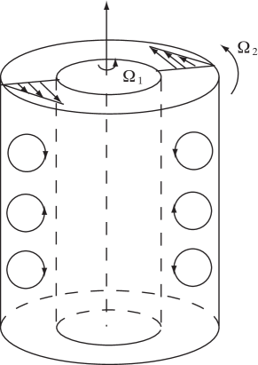
Figure 1.1. Couette Flow and Taylor vortices

There have been extensive studies for the Taylor problem from both the mathematical and physical point of view; see among many others, [16, 15, 1, 2]. Over the years, the Taylor problem, together with the Rayleigh-Bénard convection problem, has become one of the paradigms for studying nonequilibrium phase transitions and pattern formation in nonlinear sciences.

The main objective of this article is to address the dynamic transition of the Taylor-Couette flow, and and study the formation and stability in its structure of the Taylor vortices. The main technical tools are the dynamical transition theory and the geometric theory for incompressible flows, both developed recently by the authors; see [6, 11] and the references therein.

The main philosophy of the dynamic transition theory is to search for the full set of transition states, giving a complete characterization on stability and transition. The set of transition states is represented by a local attractor. Following this philosophy, the dynamic transition theory is developed to identify the transition states and to classify them both dynamically and physically. One important ingredient of this theory is the introduction of a dynamic classification scheme of phase transitions. With this classification scheme, phase transitions are classified into three types: continuous (Type-I), jump (Type-II) and mixed (Type-III). The dynamic transition theory is recently developed by the authors to identify the transition states and to classify them both dynamically and physically; see above references for details. The theory is motivated by phase transition problems in nonlinear sciences. Namely, the mathematical theory is developed under close links to the physics, and in return the theory is applied to the physical problems, although more applications are yet to be explored. With this theory, many long standing phase transition problems are either solved or become more accessible, providing new insights to both theoretical and experimental studies for the underlying physical problems.

For simplicity, we focus in this article on the $z$-periodic boundary condition, which is an approximate description for the case where the ratio $L/(r_{2}-r_{1})$ between the height $L$ and the gap $r_{2}-r_{1}$ is sufficiently large. We remark that similar results hold true as well for other type of boundary conditions, as well as for three dimensional perturbations (in the narrow-gap case); we refer the interested readers to [11] for further details.

The main results obtained are as follows.

First, we show that the system always undergoes a dynamic transition as the Taylor number $T$ crosses the critical Taylor number $T_{c}$. The types of the transition can be either continuous (Type-I) or jump (Type-II), and are dictated precisely by the sign of a nondimensional parameter $R$, given completely by the first eigenvectors, the ratio of the angular velocity of the outer and inner cylinders $\mu$, and and the ratio of the radii of the inner and outer cylinders $\eta$.

Second, when $R<0$, the transition is continuous, and the critical exponent of the phase transition, i.e., the exponent in the expression of bifurcated solutions, is $\beta=1/2$. Moreover, there is only one critical Taylor number $T_{c}$ such that the secondary flow tends to the basic flow (Couette flow) as $T\rightarrow T_{c}$.

Also, for the narrow-gap case, the parameter $R$ defined by (3.24) is negative: $R<0$, provided the two coaxial cylinders rotating in the same direction, including the case where the outer cylinder does not rotate.

Third, when $R>0$, the transition is a jump transition, leading to more drastic changes, coexistence of metastable states, and potentially more chaotic/turbulent behavior. In particular, there are two critical Taylor numbers $T_{c}$ and $T^{*}$ with $T^{*}<T_{c}$. When $T^{*}<T<T_{c}$, the system has two metastable states $\Sigma_{0}$, the trivial Couette flow and $\Sigma^{T}$, a local attractor away from the Couette flow. When $T>T_{c}$, the solution always moves away from the basic Couette flow to a more chaotic/turbulent regime, represented by the local attractor $\Sigma^{T}$.

Fourth, the theoretic analysis carried out in this article shows that a street of vortices appear in the secondary flow for the narrow-gap case with $\mu\rightarrow 1$. Thus the theoretic results are in agreement with the Taylor experiments.

The article is organized as follows. The partial differential equation model and the set-up are given in Section 2, and the main dynamic transition theorems are given in Section 3. Explicit expressions of the parameter $R$ for determining the types of transitions are further discussed in Section 4. The formation and structural stability of the Taylor vortices are addressed further in Section 5, and the main theorems are proved in Section 6.

2. The Taylor Problem

2.1. Couette flow and Taylor vortices

Consider an incompressible viscous fluid between two coaxial cylinders. Let $r_{1}$ and $r_{2}$ $(r_{2}>r_{1})$ be the radii of the two cylinders, $\Omega_{1}$ and $\Omega_{2}$ the angular velocities of the inner and the outer cylinders respectively, and

(2.1) $$\mu=\Omega_{2}/\Omega_{1},\ \ \ \ \eta=r_{1}/r_{2}.$$

The nondimensional Taylor number is defined by

(2.2) $$T=\frac{4h^{4}\Omega^{2}_{1}}{\nu^{2}},$$

where $\nu>0$ is the kinematic viscosity, and $h$ is the vertical length scale.

There exists a basic steady state flow, called the Couette flow. In the cylindrical polar coordinate $(r,\theta,z)$, the Couette flow is defined by

(2.3) $$\left.\begin{aligned} &(u_{r},u_{\theta},u_{z},p)=\left(0,V(r),0,\rho\int\frac{1}{r}V^{2}(r)dr\right),\\ &V(r)=ar+b/r,\end{aligned}\right.$$

where $(u_{r},u_{\theta},u_{z})$ is the velocity field, $p$ is the pressure, and $a,b$ are constants. It follows from the boundary conditions that

$$V(r_{1})=\Omega_{1}r_{1},\ \ \ \ V(r_{2})=\Omega_{2}r_{2},$$

and the constants a and $b$ in (2.3) are given by

$$a=-\Omega_{1}\eta^{2}\frac{1-\mu/\eta^{2}}{1-\eta^{2}},\ \ \ \ b=\Omega_{1}\frac{r^{2}_{1}(1-\mu)}{1-\eta^{2}}.$$

where $\mu$ and $\eta$ are given by (2.1).

Based on the Rayleigh criterion, when $\mu>\eta^{2}$, the Couette flow is always stable at a distribution of angular velocities

$$\Omega(r)=a+b/r^{2}\qquad\text{ for }r_{1}<r<r_{2}.$$

However, when $\mu<\eta^{2}$, the situation is different. As in the Taylor experiments, consider the case where the gap $r_{2}-r_{1}$ is much smaller than the mean radius $r_{0}=1/2(r_{1}+r_{2})$, namely,

$$r_{2}-r_{1}\ll(r_{1}+r_{2})/2,$$

and the two cylinders rotate in the same direction. If the Taylor number $T$ in (2.2) satisfies $T<T_{c}$, then the Couette flow (2.3) is stable, and if $T_{c}<T<T_{c}+\varepsilon$ for some $\varepsilon>0$, a street of vortices along the $z$-axis, called the Taylor vortices, emerge abruptly from the basic flow, as shown in Figure 1.1, and the corresponding flow pattern is radically symmetric and structurally stable.

When the gap $r_{2}-r_{2}$ is not small than $r_{0}=1/2(r_{1}+r_{2})$, or when the cylinders rotate in the opposite directions, the phenomena one observes are much more complex; see [1] for details.

Hence, in this section we always assume the condition

(2.4) $$\eta^{2}>\mu\geq 0.$$

2.2. Governing equations

The hydrodynamic equations governing an incompressible viscous fluid between two coaxial cylinders are the Navier-Stokes equations. In the cylindrical polar coordinates $(r,\theta,z)$, they are given by

(2.5) $$\frac{\partial u_{r}}{\partial t}+(u\cdot\nabla)u_{r}-\frac{u^{2}_{\theta}}{r}=\nu\left(\Delta u_{r}-\frac{2}{r^{2}}\frac{\partial u_{\theta}}{\partial\theta}-\frac{u_{r}}{r^{2}}\right)-\frac{1}{\rho}\frac{\partial p}{\partial r},$$

$$\frac{\partial u_{\theta}}{\partial t}+(u\cdot\nabla)u_{\theta}+\frac{u_{r}u_{\theta}}{r}=\nu\left(\Delta u_{\theta}+\frac{2}{r^{2}}\frac{\partial u_{r}}{\partial\theta}-\frac{u_{\theta}}{r^{2}}\right)-\frac{1}{r\rho}\frac{\partial p}{\partial\theta},$$

$$\frac{\partial u_{z}}{\partial t}+(u\cdot\nabla)u_{z}=\nu\Delta u_{z}-\frac{1}{\rho}\frac{\partial p}{\partial z},$$

$$\frac{\partial(ru_{r})}{\partial r}+\frac{\partial u_{\theta}}{\partial\theta}+\frac{\partial(ru_{z})}{\partial z}=0,$$

where $\nu$ is the kinematic viscosity, $\rho$ is the density, $u=(u_{r},u_{\theta},u_{z})$ is the velocity field, $p$ is the pressure function, and

$$u\cdot\nabla=u_{r}\frac{\partial}{\partial r}+\frac{u_{\theta}}{r}\frac{\partial}{\partial\theta}+u_{z}\frac{\partial}{\partial z},$$

$$\Delta=\frac{\partial^{2}}{\partial r^{2}}+\frac{1}{r}\frac{\partial}{\partial r}+\frac{1}{r^{2}}\frac{\partial^{2}}{\partial\theta^{2}}+\frac{\partial^{2}}{\partial z^{2}}.$$

Then it is easy to see that the Couette flow (2.3) is a steady state solution of (2.5). In order to investigate its stability and transitions, we need to consider the perturbed state of (2.3):

$$u_{r},u_{\theta}+V(r),u_{z},p+\rho\int\frac{1}{r}v^{2}(r)dr.$$

The perturbed equations read

(2.6) $$\left.\begin{aligned} &\frac{\partial u_{r}}{\partial t}+(u\cdot\nabla)u_{r}-\frac{u^{2}_{\theta}}{r}=\nu\left(\Delta u_{r}-\frac{2}{r^{2}}\frac{\partial u_{\theta}}{\partial\theta}-\frac{u_{r}}{r^{2}}\right)-\frac{1}{\rho}\frac{\partial p}{\partial r}\\ &\qquad\qquad\qquad+\frac{2V(r)}{r}u_{\theta}-\frac{V(r)}{r}\frac{\partial u_{r}}{\partial\theta},\\ &\frac{\partial u_{\theta}}{\partial t}+(u\cdot\nabla)u_{\theta}+\frac{u_{\theta}u_{r}}{r}=\nu\left(\Delta u_{\theta}+\frac{2}{r^{2}}\frac{\partial u_{r}}{\partial\theta}-\frac{u_{\theta}}{r^{2}}\right)\\ &\qquad\qquad\qquad-\frac{1}{r\rho}\frac{\partial p}{\partial\theta}-(V^{\prime}+\frac{V}{r})u_{r}-\frac{V}{r}\frac{\partial u_{\theta}}{\partial\theta},\\ &\frac{\partial u_{z}}{\partial t}+(u\cdot\nabla)u_{z}=\nu\Delta u_{z}-\frac{1}{\rho}\frac{\partial p}{\partial z}-\frac{V}{r}\frac{\partial u_{z}}{\partial\theta},\\ &\frac{\partial(ru_{z})}{\partial z}+\frac{\partial(ru_{r})}{\partial r}+\frac{\partial u_{\theta}}{\partial\theta}=0.\end{aligned}\right.$$

To derive the nondimensional form of equations (2.6), let

$$(x,t)=(hx^{\prime},h^{2}t^{\prime}/\nu) (x=(r,r\theta,z)),$$

$$(u,p)=(\nu u^{\prime}/h,\rho\nu^{2}p^{\prime}/h^{2}) (u=(u_{r},u_{\theta},u_{z})).$$

Omitting the primes, we obtain the nondimensional form of (2.6) as follows:

(2.7) $$\left.\begin{aligned} &\frac{\partial u_{r}}{\partial t}=\Delta u_{r}-\frac{2}{r^{2}}\frac{\partial u_{\theta}}{\partial\theta}-\frac{u_{r}}{r^{2}}-(u\cdot\nabla)u_{r}+\frac{u^{2}_{\theta}}{r}-\frac{\partial p}{\partial r}\\ &\qquad\qquad-\sqrt{T}\left(\frac{\eta^{2}-\mu}{1-\eta^{2}}-\frac{1-\mu}{1-\eta^{2}}\frac{r^{2}_{1}}{r^{2}}\right)\left(u_{\theta}-1/2\frac{\partial u_{r}}{\partial\theta}\right),\\ &\frac{\partial u_{\theta}}{\partial t}=\Delta u_{\theta}+\frac{2}{r^{2}}\frac{\partial u_{r}}{\partial\theta}-\frac{u_{\theta}}{r^{2}}-(u\cdot\nabla)u_{\theta}-\frac{u_{\theta}u_{r}}{r}-\frac{1}{r}\frac{\partial p}{\partial\theta}\\ &\qquad\qquad+\sqrt{T}\frac{\eta^{2}-\mu}{1-\eta^{2}}u_{r}+\frac{\sqrt{T}}{2}\left(\frac{\eta^{2}-\mu}{1-\eta^{2}}-\frac{1-\mu}{1-\eta^{2}}\frac{r^{2}_{1}}{r^{2}}\right)\frac{\partial u_{\theta}}{\partial\theta},\\ &\frac{\partial u_{z}}{\partial t}=\Delta u_{z}-(u\cdot\nabla)u_{z}-\frac{\partial p}{\partial z}+\frac{\sqrt{T}}{2}\left(\frac{\eta^{2}-\mu}{1-\eta^{2}}-\frac{1-\mu}{1-\eta^{2}}\frac{r^{2}_{1}}{r^{2}}\right)\frac{\partial u_{z}}{\partial\theta},\\ &\frac{\partial(ru_{z})}{\partial z}+\frac{\partial(ru_{r})}{\partial r}+\frac{\partial u_{\theta}}{\partial\theta}=0,\end{aligned}\right.$$

where $T$ is the Taylor number as defined in (2.2).

The nondimensional domain for (2.7) is

$$\Omega=(l_{1},l_{2})\times(0,2\pi)\times(0,L),$$

where $l_{i}=r_{i}/h$ $(i=1,2)$, and $L$ is the height of the fluid between the two cylinders. The initial value condition for (2.7) is given by

(2.8) $$u(r,\theta,z,0)=u_{0}(r,\theta,z).$$

There are different physically sound boundary conditions. In the $\theta$-direction it is periodic

(2.9) $$u(r,\theta+2k\pi,z)=u(r,\theta,z),\ \ \ \ \forall k\in\mathbb{Z}.$$

In the radical direction, there is the rigid boundary condition

(2.10) $$u=(u_{z},u_{r},u_{\theta})=0,\ \ \ \ \text{at}\ \ \ \ r=l_{1},l_{2}.$$

At the top and bottom in the $z$-direction $(z=0,L)$, either the free boundary condition or the rigid boundary condition or the periodic boundary condition can be used:

Dirichlet Boundary Condition:

(2.11) $$u=(u_{r},u_{\theta},u_{z})=0\ \ \ \ \text{at}\ \ \ \ z=0,L;$$

Free-Slip Boundary Condition:

(2.12) $$u_{z}=0,\ \ \ \ \frac{\partial u_{r}}{\partial z}=\frac{\partial u_{\theta}}{\partial z}=0\ \ \ \ \text{at}\ \ \ \ z=0,L;$$

Free-Rigid Boundary Condition:

(2.13) $$\left.\begin{aligned} &u_{z}=0,\frac{\partial u_{r}}{\partial z}=\frac{\partial u_{\theta}}{\partial z}=0&&\text{at}\ z=L,\\ &u=(u_{z},u_{r},u_{\theta})=0&&\text{at}\ z=0;\end{aligned}\right.$$

Periodic Boundary Condition:

(2.14) $$u(r,\theta,z+2kL)=u(r,\theta z)\ \ \ \ \forall k\in\mathbb{Z}.$$

3. Dynamic Transitions

3.1. Functional setting

We now study the Taylor problem (2.7) with the $z$-periodic boundary condition (2.14) and with axisymmetric perturbations. Assuming that the equations (2.7) are independent of $\theta$, and taking the length scale $h=r_{2}$ in the nondimensional form, we obtain

(3.1) $$\left.\begin{aligned} &\frac{\partial u_{z}}{\partial t}=\Delta u_{z}-\frac{\partial p}{\partial z}-(\tilde{u}\cdot\nabla)u_{z},\\ &\frac{\partial u_{r}}{\partial t}=(\Delta-\frac{1}{r^{2}})u_{r}+\lambda\left(\frac{1}{r^{2}}-\kappa\right)u_{\theta}-\frac{\partial p}{\partial r}+\frac{u^{2}_{\theta}}{r}-(\tilde{u}\cdot\nabla)u_{r},\\ &\frac{\partial u_{\theta}}{\partial t}=\left(\Delta-\frac{1}{r^{2}}\right)u_{\theta}+\lambda\kappa u_{r}-\frac{u_{r}u_{\theta}}{r}-(\tilde{u}\cdot\nabla)u_{\theta},\\ &\frac{\partial(ru_{z})}{\partial z}+\frac{\partial(ru_{r})}{\partial r}=0,\end{aligned}\right.$$

where $\lambda=\sqrt{T}$, $T$ is the Taylor number, and

$$T=\frac{4r^{4}_{2}\Omega^{2}_{1}(1-\mu)^{2}\eta^{4}}{\nu^{2}(1-\eta^{2})^{2}}, \eta^{2}=r^{2}_{1}/r^{2}_{2},$$

$$\kappa=\frac{1-\mu/\eta^{2}}{1-\mu}, \Delta=\frac{\partial^{2}}{\partial r^{2}}+\frac{1}{r}\frac{\partial}{\partial r}+\frac{\partial^{2}}{\partial z^{2}},$$

$$(\widetilde{u}\cdot\nabla)=u_{r}\,\frac{\partial}{\partial r}+u_{z}\,\frac{\partial}{\partial z}.$$

The nondimensional domain is $M=(\eta,1)\times(0,L)$, and the boundary conditions take (2.10) and (2.14), i.e.,

(3.2) $$\left.\begin{aligned} &u=(u_{z},u_{r},u_{\theta})=0\qquad\text{at}\ r=\eta,1,\\ &u\ \text{is\ periodic\ with\ period}\ L\ \text{in\ the}\ z-\text{direction}.\end{aligned}\right.$$

The initial value condition is

(3.3) $$u=u_{0}(r,z)\ \ \ \ \text{at}\ \ \ \ t=0.$$

For the Taylor problem (3.1)-(3.3), we set

$$H=\left\{u=(\tilde{u},u_{\theta})\in L^{2}(M)^{3}\left|\begin{array}[]{l}\text{div}(r\tilde{u})=0,u_{r}=0\ \text{at}\ r=\eta,1,\ \text{and}\\ u\ \text{is}\ L-\text{periodic\ in\ the}\ z-\text{direction}\end{array}\right.\right\}$$

$$H_{1}=\left\{u\in H^{2}(M)^{3}\bigcap H\ |\ u\ \text{satisfies}\ (\ref{9.146})\right\},$$

and the inner product of $H$ is defined by

$$(u,v)_{H}=\int_{M}u\cdot vrdzdr.$$

Let the linear operator $L_{\lambda}=-A+\lambda B:H_{1}\rightarrow H$ and nonlinear operator $G:H_{1}\rightarrow H$ be defined by

(3.5) $$\left.\begin{aligned} &Au=-P\left(\Delta u_{z},\left(\Delta-\frac{1}{r^{2}}\right)u_{r},\left(\Delta-\frac{1}{r^{2}}\right)u_{\theta}\right),\\ &Bu=P\left(0,\left(\frac{1}{r^{2}}-\kappa\right)u_{\theta},\kappa u_{r}\right),\\ &G(u)=-P\left((\tilde{u}\cdot\nabla)u_{z},(\tilde{u}\cdot\nabla)u_{r}-\frac{u^{2}_{\theta}}{r},(\tilde{u}\cdot\nabla)u_{\theta}+\frac{u_{\theta}u_{r}}{r}\right),\end{aligned}\right.$$

where $P:L^{2}(M)^{3}\rightarrow H$ is the Leray projection. Thus the Taylor problem (3.1)-(3.3) is rewritten in the abstract form

(3.6) $$\left.\begin{aligned} &\frac{du}{dt}=L_{\lambda}u+G(u),\\ &u(0)=u_{0}.\end{aligned}\right.$$

For simplicity, let $G:H_{1}\rightarrow H$ be the corresponding bilinear operator defined by

$$G(u,v)=-P\left((\tilde{u}\cdot\nabla)v_{z},(\tilde{u}\cdot\nabla)u_{r}-\frac{u_{\theta}v_{\theta}}{r},(\tilde{u}\cdot\nabla)v_{\theta}+\frac{u_{\theta}v_{r}}{r}\right).$$

Then it is easy to see that

(3.7) $$(G(u,v),w)_{H}=-(G(u,w),v)_{H}.$$

3.2. Eigenvalue problem

To study the phase transition of the Taylor problem (3.1)-(3.3) it is necessary to consider the eigenvalue problem of its linearized equation. The associated eigenvalue equation of (3.6) is as follows:

(3.8) $$L_{\lambda}u=-Au+\lambda Bu=\beta(\lambda)u,$$

and the conjugate equation of (3.8) is given by

(3.9) $$L^{*}_{\lambda}u^{*}=-A^{*}u^{*}+\lambda B^{*}u^{*}=\beta(\lambda)u^{*}.$$

The equations corresponding to (3.8) are as follows

(3.10) $$\left.\begin{aligned} &\Delta u_{z}-\frac{\partial p}{\partial z}=\beta(\lambda)u_{z},\\ &\left(\Delta-\frac{1}{r^{2}}\right)u_{r}+\lambda\left(\frac{1}{r^{2}}-\kappa\right)u_{\theta}-\frac{\partial p}{\partial r}=\beta(\lambda)u_{r},\\ &\left(\Delta-\frac{1}{r^{2}}\right)u_{\theta}+\lambda\kappa u_{r}=\beta(\lambda)u_{\theta},\\ &\text{div}(r\tilde{u})=0.\end{aligned}\right.$$

The equations corresponding to (3.9) are given by

(3.11) $$\left.\begin{aligned} &\Delta u^{*}_{z}-\frac{\partial p^{*}}{\partial z}=\beta(\lambda)u^{*}_{z},\\ &\left(\Delta-\frac{1}{r^{2}}\right)u^{*}_{r}+\lambda\kappa u^{*}_{\theta}-\frac{\partial p^{*}}{\partial r}=\beta(\lambda)u^{*}_{r},\\ &\left(\Delta-\frac{1}{r^{2}}\right)u^{*}_{\theta}+\lambda\left(\frac{1}{r^{2}}-\kappa\right)u^{*}_{r}=\beta(\lambda)u^{*}_{\theta},\\ &\text{div}(r\tilde{u}^{*})=0.\end{aligned}\right.$$

Both (3.10) and (3.11) are supplemented with the boundary condition (3.2).

We start with the principle of exchange of stability (PES). It is known that for each given period $L$, there is a $\lambda^{*}_{0}=\lambda_{0}(L)$ such that the eigenvalues $\beta_{j}(\lambda)$ $(j=1,2,\cdots)$ of (3.10) with (3.2) near $\lambda=\lambda^{*}_{0}$ satisfy that $\beta_{1}(\lambda),\cdots,\beta_{m}(\lambda)$ $(m\geq 1)$ are real, and

(3.12) $$\left.\begin{aligned} &\beta_{i}(\lambda)\left\{\begin{aligned} &<0&&\text{if }\ \lambda<\lambda^{*}_{0},\\ &=0&&\text{if }\ \lambda=\lambda^{*}_{0}\end{aligned}\right.&&\text{for }1\leq i\leq m,\\ &\text{Re}\beta_{j}(\lambda^{*}_{0})<0&&\text{for }j\geq m+1.\end{aligned}\right.$$

In addition, there is a period $L^{\prime}>0$ such that

(3.13) $$\lambda_{0}=\lambda_{0}(L^{\prime})=\min\limits_{L>0}\lambda_{0}(L).$$

Thanks to [16, 15], for $\mu=\Omega_{1}/\Omega_{2}\geq 0$ the multiplicity $m=2$ in (3.12) at $\lambda_{0}=\lambda_{0}(L^{\prime})$; see also [3, 14].

In this section, we always take $L^{\prime}$ as the period given by (3.13), and define the following number as the critical Taylor number:

$$T_{c}=\lambda^{2}_{0}(L^{\prime}).$$

For simplicity, omitting the prime we denote $L^{\prime}$ by $L$.

By (3.12) and (3.13), to verify the PES it suffices to prove that for $\lambda>\lambda_{0}$,

(3.14) $$\beta_{i}(\lambda)>0\qquad\forall 1\leq i\leq m.$$

To this end, we need to derive the eigenvectors of (3.10) and (3.11) at $\beta_{i}(\lambda_{0})=0$ $(i=1,2).$

It is readily to check that the eigenvectors of (3.10) with (3.2) corresponding to $\beta_{i}(\lambda_{0})=0$ $(i=1,2)$ are given by

(3.15) $$\psi_{1}=(\psi_{z},\psi_{r},\psi_{\theta})=(-\sin az\ D_{*}h(r),a\cos az\ h(r),\cos az\ \varphi(r)),$$

(3.16) $$\tilde{\psi}_{1}=(\tilde{\psi}_{z},\tilde{\psi}_{r},\tilde{\psi}_{\theta})=(\cos az\ D_{*}h(r),a\sin az\ h(r),\sin az\ \varphi(r)),$$

where $(h(r),\varphi(r))$ satisfies

(3.17) $$\left.\begin{aligned} &(DD_{*}-a^{2})^{2}h=a^{2}\lambda_{0}\left(\frac{1}{r^{2}}-\kappa\right)\varphi,\\ &(DD_{*}-a^{2})\varphi=-\lambda_{0}\kappa h,\\ &(h,Dh,\varphi)=0&&\text{at }r=\eta,1,\end{aligned}\right.$$

and

$$D=\frac{d}{dr},\ \ \ \ D_{*}=\frac{d}{dr}+\frac{1}{r},\ \ \ \ a=\frac{2\pi}{L}.$$

The dual eigenvectors of (3.11) with (3.2) read

(3.18) $$\psi^{*}_{1}=(\psi^{*}_{z},\psi^{*}_{r},\psi^{*}_{\theta})=(-\sin az\ D_{*}h^{*}(r),a\cos az\ h^{*}(r),\cos az\ \varphi^{*}(r)),$$

(3.19) $$\tilde{\psi}^{*}_{1}=(\tilde{\psi}^{*}_{z},\tilde{\psi}^{*}_{r},\tilde{\psi}^{*}_{\theta})=(\cos az\ D_{*}h^{*}(r),a\sin az\ h^{*}(r),\sin az\ \varphi^{*}(r)),$$

where $(h^{*},\varphi^{*})$ satisfies that

(3.20) $$\left.\begin{aligned} &(DD_{*}-a^{2})^{2}h^{*}=\lambda_{0}\kappa\varphi^{*},\\ &(DD_{*}-a^{2})\varphi^{*}=-a^{2}\lambda_{0}\left(\frac{1}{r^{2}}-\kappa\right)h^{*},\\ &(h^{*},Dh^{*},\varphi^{*})=0&&\text{at }r=\eta,1.\end{aligned}\right.$$

The following lemma shows that the PES is valid for the Taylor problem (3.1)-(3.3) with $\mu\geq 0$.

Lemma 3.1.

If $\mu\geq 0$, then the first eigenvalues $\beta_{i}(\lambda)$ $(1\leq i\leq m)$ of (3.10) are real with multiplicity $m=2$ near $\lambda=\lambda_{0}=\sqrt{T_{c}}$, and the first eigenvectors at $\lambda=\lambda_{0}$ are given by (3.15) and (3.16). Moreover, the eigenvalues $\beta_{j}(\lambda)$ $(j=1,2,\cdots)$ satisfy the conditions (5.4) and (5.5) at $\lambda=\lambda_{0}$, i.e., the PES holds true at the critical Taylor number $T_{c}$.

Proof.

We only need to prove (3.14). By Theorem 2.1 in [9], it suffices to verify that

(3.21) $$(B\psi_{1},\psi^{*}_{1})_{H}\neq 0,\ \ \ \ (B\tilde{\psi}_{1},\tilde{\psi}^{*}_{1})_{H}\neq 0.$$

We infer from (3.5), (3.15), (3.16), (3.18), and (3.19) that

$$(B\psi_{1},\psi^{*}_{1})_{H} = (B\tilde{\psi}_{1},\tilde{\psi}^{*}_{1})_{H}$$

$$= \int^{L}_{0}\int^{1}_{\eta}r\left[\left(\frac{1}{r^{2}}-\kappa\right)\psi_{\theta}\psi^{*}_{r}+\kappa\psi_{r}\psi^{*}_{\theta}\right]dzdr$$

$$= \frac{La}{2}\int^{1}_{\eta}r\left[\left(\frac{1}{r^{2}}-\kappa\right)h\varphi^{*}+\kappa\varphi h^{*}\right]dr.$$

Since $\mu\geq 0$, by (2.4), we have $0<\kappa<1$ and $\frac{1}{r^{2}}-\kappa>0$ for $\eta<r<1$. On the other hand, we know that the first eigenvectors $(h(r),\varphi(r))$ of (3.17) and $(h^{*}(r),\varphi^{*}(r))$ of (3.20) at $\lambda=\lambda_{0}$ are positive; see [15, 3, 14]:

(3.23) $$h(r)>0,\ \ \ \ \varphi(r)>0,\ \ \ \ h^{*}(r)>0,\ \ \ \ \varphi^{*}(r)>0\ \ \ \ \forall\eta<r<1.$$

Thus (3.21) follows from (3.2) and (3.23). The proof is complete. ∎

3.3. Phase transition theorems

Here we always assume that the first eigenvalue of (3.10) with (3.2) is real with multiplicity $m=2$, i.e., the first eigenvalue $\lambda_{0}$ of (3.17) is simple, and the PES holds true. By Lemma 3.1, this assumption is valid for all $\mu\geq 0$ and $0<\eta<1.$

Let $\psi_{1}$ and $\psi^{*}_{1}$ be given by (3.15) and (3.18). We define a number $R$ by

(3.24) $$R=\frac{1}{(\psi_{1},\psi^{*}_{1})_{H}}\left[(G(\Phi,\psi_{1}),\psi^{*}_{1})_{H}+(G(\psi_{1},\Phi),\psi^{*}_{1})_{H}\right],$$

where $\Phi\in H_{1}$ is defined by

(3.25) $$(A-\lambda_{0}B)\Phi=G(\psi_{1},\psi_{1}).$$

Here the operator $A,B$ and $G$ are as in (3.5). The solution $\Phi$ of (3.25) exists because $G(\psi,\psi_{1})$ is orthogonal with $\psi^{*}_{1}$ and $\tilde{\psi}^{*}_{1}$ in $H$.

The following results characterize the dynamical properties of phase transitions for the Taylor problem with the $z$-periodic boundary condition.

Theorem 3.1.

If the number $R<0$ in (3.24), then the Taylor problem (3.1)-(3.3) has a Tyep-I (continuous) transition at the critical Taylor number $T=T_{c}$ or $\lambda=\lambda_{0}$, and the following assertions holds true:

• When the Taylor number $T\leq T_{c}$ or $\lambda\leq\lambda_{0}$, the steady state $u=0$ is locally asymptotically stable.

• The problem bifurcates from $(u,\lambda)=(0,\lambda_{0})$ (or from $(u,T)=(0,T_{c}))$ to an attractor ${\mathcal{A}}_{\lambda}$ homeomorphic to a circle $S^{1}$ on $\lambda_{0}<\lambda$, which consists of steady states of this problem.

• Any $u\in{\mathcal{A}}_{\lambda}$ can be expressed as

  $$u=|\beta_{1}(\lambda)/R|^{1/2}v+o(|\beta_{1}|^{1/2}),$$

  $$v=x\psi_{1}+y\tilde{\psi}_{1},$$

  $$x^{2}+y^{2}=1,$$

  where $\psi_{1},\tilde{\psi}_{1}$ are given in (3.15) and (3.18).

• There is an open set $U\subset H$ with $0\in U$ such that ${\mathcal{A}}_{\lambda}$ attracts $U\setminus\Gamma$, where $\Gamma$ is the stable manifold of $u=0$ with codimension two in $H$.

• When $1-\mu>0$ is small, for any $u_{0}\in U\setminus(\Gamma\bigcup\widetilde{H})$, there exists a time $t_{0}\geq 0$ such that for any $t>t_{0}$, the vector field $\tilde{u}(t,u_{0})=(u_{z},u_{r})$ is topologically equivalent to one of the patterns shown in Figure 3.1, where $u=(\tilde{u}(t,u_{0}),u_{\theta}(t,u_{0}))$ is the solution of (3.1)-(3.3), and

  $$\widetilde{H}=\{u=(u_{z},u_{r},u_{\theta})\in H|\ \int^{L}_{0}\int^{1}_{\eta}ru_{z}drdz=0\}.$$

• When $1-\mu>0$ is small, for any $u_{0}\in(U\bigcap\tilde{H})\setminus\Gamma$, there exists a time $t_{0}\geq 0$ such that for any $t>t_{0},\tilde{u}(t,u_{0})=(u_{z},u_{r})$ is topologically equivalent to the structure as shown in Figure 3.2.

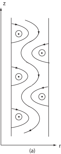
Figure 3.1. Taylor vortices with a cross-channel flow.

Figure 3.2. Taylor vortices without a cross-channel flow.

Theorem 3.2.

For the case where $R>0$, the transition of the Taylor problem (3.1)-(3.3) at $T=T_{c}$ is of Type-II. Moreover, the Taylor problem has a singularity separation at $T^{*}<T_{c}$ $(\lambda^{*}<\lambda_{0})$. More precisely we have the following assertions:

• There exists a number $\lambda^{*}$ $(0<\lambda^{*}<\lambda_{0})$ such that the problem generate a circle $\Sigma^{*}=S^{1}$ at $\lambda=\lambda^{*}$ consisting of singular points, and bifurcates from $(\Sigma^{*},\lambda^{*})$ on $\lambda^{*}<\lambda$ to at least two branches of circles $\Sigma^{\lambda}_{1}$ and $\Sigma^{\lambda}_{2}$, each consisting of steady states satisfying

  $$\lim_{\lambda\to\lambda_{0}}\Sigma^{1}_{\lambda}=\{0\},$$

  $$\text{dist}\left(\Sigma^{\lambda}_{2},0\right)=\min_{u\in\Sigma^{\lambda}_{2}}\|u\|_{H}>0 \text{at}\ \ \ \ \lambda=\lambda_{0};$$

  see Figure 3.3.

• For each $\lambda^{*}<\lambda<\lambda_{0}$, the space $H$ can be decomposed into two open sets $U^{\lambda}_{1}$ and $U^{\lambda}_{2}:H=\bar{U}^{\lambda}_{1}+\bar{U}^{\lambda}_{2}$ with $U^{\lambda}_{1}\bigcap U^{\lambda}_{2}=\emptyset,\Sigma^{\lambda}_{1}\subset\partial U^{\lambda}_{1}\bigcap\partial U^{\lambda}_{2}$ such that the problem has two disjoint attractors ${\mathcal{A}}^{\lambda}_{1}$ and ${\mathcal{A}}^{\lambda}_{2}$:

  $${\mathcal{A}}^{\lambda}_{1}=\{0\}\subset U^{\lambda}_{1},\ \ \ \ \Sigma^{\lambda}_{2}\subset{\mathcal{A}}^{\lambda}_{2}\subset U^{\lambda}_{2},$$

  and ${\mathcal{A}}^{\lambda}_{i}$ attracts $U^{\lambda}_{i}$ $(i=1,2)$.

• For $\lambda_{0}\leq\lambda$, the problem has an attractor ${\mathcal{A}}^{\lambda}$ satisfying

  $$\lim\limits_{\lambda\rightarrow\lambda_{0}}{\mathcal{A}}^{\lambda}_{2}={\mathcal{A}}^{\lambda_{0}},\ \ \ \ \text{dist}({\mathcal{A}}^{\lambda},0)>0\ \ \ \ \forall\lambda\geq\lambda_{0},$$

  and ${\mathcal{A}}^{\lambda}$ attracts $H\setminus\Gamma_{\lambda}$, where $\Gamma_{\lambda}$ is the stable manifold of $u=0$ with codimension $m_{\lambda}\geq 2$ in $H$.

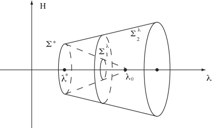
Figure 3.3. Singularity separation of circles consisting of steady states at $\lambda=\lambda^{*}$.

4. Explicit expression of the parameter $R$

4.1. General case

The parameter $R$ defined by (3.24) and (3.25) can be explicitly expressed in the following integral formula:

$$R= -\frac{1}{(\psi_{1},\psi^{*}_{1})_{H}}\Big{[}\frac{\pi}{2}\int^{1}_{\eta}rh\varphi^{*}\frac{d\phi_{0}}{dr}dr$$

$$+\int^{L}_{0}\int^{1}_{\eta}r\Big{(}(\tilde{\phi}\cdot\nabla)\psi_{z}\psi^{*}_{z}+(\tilde{\psi}\cdot\nabla)\phi_{z}\psi^{*}_{z}+(\tilde{\phi}\cdot\nabla)\psi_{r}\psi^{*}_{r}$$

$$+(\tilde{\psi}\cdot\nabla)\phi_{r}\psi^{*}_{r}+(\tilde{\phi}\cdot\nabla)\psi_{\theta}\psi^{*}_{\theta}+(\tilde{\psi}\cdot\nabla)\phi_{\theta}\psi^{*}_{\theta}$$

$$+\frac{\phi_{\theta}\psi_{r}\psi^{*}_{\theta}}{r}+\frac{\psi_{\theta}\phi_{r}\psi^{*}_{\theta}}{r}-2\frac{\psi_{\theta}\phi_{\theta}\psi^{*}_{r}}{r}\Big{)}drdz\Big{]},$$

where $\tilde{\psi}=(\psi_{z},\psi_{r}),\psi_{1}=(\psi_{z},\psi_{r},\psi_{\theta}),\psi^{*}_{1}=(\psi^{*}_{z},\psi^{*}_{r},\psi^{*}_{\theta})$ are given by (3.15) and (3.18),

$$(\psi_{1},\psi^{*}_{1})_{H}=\int^{L}_{0}\int^{1}_{\eta}r(\psi_{z}\psi^{*}_{z}+\psi_{r}\psi^{*}_{r}+\psi_{\theta}\psi^{*}_{\theta})drdz,$$

and $\phi_{0},\phi=(\phi_{z},\phi_{r},\phi_{\theta})$ satisfy

$$\left\{\begin{aligned} &DD_{*}\phi_{0}=a(\varphi D_{*}h+hD\varphi+\frac{1}{r}\varphi h),\\ &\phi_{0}|_{r=\eta,1}=0,\end{aligned}\right.$$

$$\left\{\begin{aligned} &-\Delta\phi_{z}+\frac{\partial p}{\partial z}=-1/2\sin 2azH_{1}(r),\\ &-\left(\Delta-\frac{1}{r^{2}}\right)\phi_{r}-\lambda_{0}\left(\frac{1}{r^{2}}-\kappa\right)\phi_{\theta}+\frac{\partial p}{\partial r}=-1/2\cos 2azH_{2}(r),\\ &-\left(\Delta-\frac{1}{r^{2}}\right)\phi_{\theta}-\lambda_{0}\kappa\phi_{r}=-1/2\cos 2azH_{3}(r),\\ &\text{div}(r\tilde{\phi})=0,\ \ \ \ \tilde{\phi}=(\phi_{z},\phi_{r}),\\ &\phi|_{r=\eta,1}=0.\end{aligned}\right.$$

Here $H_{i}(r),i=1,2,3$, are as in (6.9).

4.2. Narrow-gap case

We consider here the case where the gap $r_{2}-r_{1}$ is small compared to the mean radius $r_{0}=(r_{1}+r_{2})/2$ with $\mu\geq 0$ and with axisymmetric perturbations. This case is the situation investigated by [13] in 1923.

We take the length scale $h=r_{2}-r_{1}$. Then the narrow gap condition is given by

(4.1) $$1=r_{2}-r_{1}\ll(r_{1}+r_{2})/2.$$

Under the assumption (4.1), we can neglect the terms containing $r^{-n}$ $(n\geq 1)$ in (2.7). In addition, by (4.1) we have

$$-\sqrt{T}\left(\frac{\eta^{2}-\mu}{1-\eta^{2}}-\frac{1-\mu}{1-\eta^{2}}\frac{r^{2}_{1}}{r^{2}}\right) = \sqrt{T}\left(1-\frac{1-\mu}{1-\eta^{2}}\frac{r^{2}-r^{2}_{1}}{r^{2}}\right)$$

$$\simeq \sqrt{T}(1-(1-\mu)(r-r_{1})).$$

Let

(4.2) $$\alpha=\frac{\eta^{2}-\mu}{1-\eta^{2}}.$$

Replacing $u_{\theta}$ by $\sqrt{\alpha}u_{\theta}$, and assuming the perturbations are axi-symmetric and are independent of $\theta$, we obtain from (2.7):

(4.3) $$\left.\begin{aligned} &\frac{\partial u_{z}}{\partial t}+(\tilde{u}\cdot\nabla)u_{z}=\Delta u_{z}-\frac{\partial p}{\partial z},\\ &\frac{\partial u_{r}}{\partial t}+(\tilde{u}\cdot\nabla)u_{r}=\Delta u_{r}-\frac{\partial p}{\partial r}+\sqrt{\alpha T}(1-(1-\mu)(r-r_{1}))u_{\theta},\\ &\frac{\partial u_{\theta}}{\partial t}+(\tilde{u}\cdot\nabla)u_{\theta}=\Delta u_{\theta}+\sqrt{\alpha T}u_{r},\\ &\frac{\partial u_{r}}{\partial r}+\frac{\partial u_{z}}{\partial z}=0,\end{aligned}\right.$$

where

$$\Delta=\frac{\partial^{2}}{\partial r^{2}}+\frac{\partial^{2}}{\partial z^{2}},\ \ \ \ (\tilde{u}\cdot\nabla)=u_{r}\frac{\partial}{\partial r}+u_{z}\frac{\partial}{\partial z}.$$

In this case, the spatial domain is $M=(r_{1},r_{1}+1)\times(0,L)$. For convenience, we consider here the Dirichlet boundary condition

(4.4) $$u|_{\partial M}=0.$$

The initial value condition is axisymmetric, and given by

(4.5) $$u=u_{0}(r,z)\ \ \ \ \text{at}\ \ \ \ t=0.$$

The linearized equations of (4.3) read

(4.6) $$\left.\begin{aligned} &-\Delta u_{z}+\frac{\partial p}{\partial z}=0,\\ &-\Delta u_{r}+\frac{\partial p}{\partial r}=\lambda u_{\theta}-\lambda(1-\mu)(r-r_{1})u_{\theta},\\ &-\Delta u_{\theta}=\lambda u_{r},\\ &\frac{\partial u_{r}}{\partial r}+\frac{\partial u_{z}}{\partial z}=0,\end{aligned}\right.$$

where $\lambda=\sqrt{\alpha T},T$ is the Taylor number given by (2.2).

Let $\lambda_{1}>0$ be the first eigenvalue of (4.6) with (4.4). We call

(4.7) $$T_{c}=\lambda^{2}_{1}/\alpha,$$

the critical Taylor number, where $\alpha$ is given by (4.2).

As $\mu\rightarrow 1$, equations (4.6) are reduced to the following symmetric linear equations:

(4.8) $$\left.\begin{aligned} &-\Delta u_{z}+\frac{\partial p}{\partial z}=0,\\ &-\Delta u_{r}+\frac{\partial p}{\partial r}=\lambda u_{\theta},\\ &-\Delta u_{\theta}=\lambda u_{r},\\ &\frac{\partial u_{z}}{\partial z}+\frac{\partial u_{r}}{\partial r}=0.\end{aligned}\right.$$

Let the first eigenvalue $\lambda_{0}>0$ of (4.8) with (4.4) have multiplicity $m\geq 1$, the corresponding eigenfunctions be $v_{i}$ $(i=1,\cdots,m)$, and the corresponding eigenspace be

$$E_{0}=\text{span}\{v_{i}\ |\ 1\leq i\leq m\}.$$

We remark here that under conditions (2.4) and (4.1), the condition $\mu\rightarrow 1$ can be equivalently replaced by

(4.9) $$r_{1}=(2+\delta)/(1-\mu),$$

for some $\delta>0$. In this case the parameter $\alpha$ in (4.2) is

$$\alpha=(\eta^{2}-\mu)/(1-\eta^{2})\simeq\delta/2.$$

When the conditions (4.1) and (4.9) hold true, $\mu\rightarrow 1$ and $r_{1}\rightarrow\infty$. In this case the equations (3.1) are replaced by (4.3), and the linearized equations of (4.3) reduces to the symmetric linear system (4.8). For the approximate problem (4.8) with (3.2), we use $R_{0}$ to denote the number $R$ defined by (3.24) and (3.25):

$$R_{0}=\frac{1}{\|\psi_{1}\|^{2}}\left[(G(\Phi,\psi_{1}),\psi_{1})+G(\psi_{1},\Phi),\psi_{1})_{H}\right].$$

Here $\psi_{1}$ is given by (3.15) with $(h,\varphi)$ satisfying

$$\left.\begin{aligned} &(D^{2}-a^{2})^{2}h=\lambda_{0}\varphi,\\ &(D^{2}-a^{2})\varphi=-\lambda_{0}h,\\ &h=Dh=0,\varphi=0&&\text{at}\ \ \ \ r=1,\eta,\end{aligned}\right.$$

and $\Phi$ is defined by

(4.10) $$\left.\begin{aligned} &(A-\lambda_{0}B_{0})\Phi=G(\psi_{1},\psi_{1}),\\ &B_{0}\Phi=P(0,\Phi_{\theta},\Phi_{r}).\end{aligned}\right.$$

By (3.7) we have

$$(G(\Phi,\psi_{1}),\psi_{1})_{H}=0,$$

$$(G(\psi_{1},\Phi),\psi_{1})_{H}=-(G(\psi_{1},\psi_{1}),\Phi)_{H}.$$

Hence, we infer from (4.10) that

$$R_{0} = -\frac{1}{\|\psi_{1}\|^{2}}(G(\psi_{1},\psi_{1}),\Phi)$$

$$= -\frac{1}{\|\psi_{1}\|^{2}}((A-\lambda_{0}B_{0})\Phi,\Phi).$$

We see that $A-\lambda_{0}B_{0}$ is symmetric and semi-positive definite, and

$$G(\psi_{1},\psi_{1})\bot\text{Ker}(A-\lambda_{0}B_{0}),\ \ \ \ \Phi\bot\text{Ker}(A-\lambda_{0}B_{0}).$$

Therefore it follows that

$$R_{0}=-\frac{1}{\|\psi_{1}\|^{2}}((A-\lambda_{0}B_{0})^{1/2}\Phi,(A-\lambda_{0}B_{0})^{1/2}\Phi)_{H}<0.$$

On the other hand, it is known that the number $R(\mu)$ in (3.24) is continuous on $\mu$, and

$$R(\mu)\rightarrow R_{0}\ \ \ \ \text{as}\ \ \ \ \mu\rightarrow 1.$$

Hence we derive the following conclusion.

Theorem 4.1.

For the Taylor problem (3.1)-(3.3) there exist $\mu_{0}<1$ and $0<\eta_{0}<1$ such that for any $\mu_{0}<\mu<1$ and $\eta_{0}<\eta<1$ with $\mu<\eta^{2}$, the parameter $R=R(\mu,\eta)$ defined by (3.24) is negative, i.e.,

$$R(\mu,\eta)<0,\ \ \ \ \forall\mu_{0}<\mu<1,\ \ \ \ \eta_{0}<\eta<1.$$

Consequently, the conclusions in Theorem 3.1 hold true.

5. Formation of the Taylor vortices and Structural Stability

Assertions (5) and (6) in Theorem 3.1 provide an asymptotic structure of the solutions in the physical space when the gap $r_{2}-r_{1}$ is small, as observed in the experiments. However, for general parameters $\eta$ and $\mu$ we can not give the precisely theoretic results, and only present some qualitative description. Here we consider two general cases as follows.

Case: $\mu\geq 0$. Following [16, 15], for the eigenvector $(h,\varphi)$ of (3.17) the function $h$ can be taken as positive and has a unique maximum point in the interval $(\eta,1)$. Therefore, for the eigenvectors defined by (3.15) and (3.16), the vector fields $(\psi_{z},\psi_{r})$ and $(\tilde{\psi}_{z},\tilde{\psi}_{r})$ are divergence-free and have the topological structure as shown in Figure 3.2. Hence to obtain Assertions (5) and (6) in Theorem 3.1 for any $\mu\geq 0$ it suffices to prove that

(5.1) $$h^{\prime\prime}(r)\neq 0\ \ \ \ \text{at}\ \ \ \ r=r_{0},1,\eta,$$

where $r_{0}\in(\eta,1)$ is the maximum point of $h$. We conjecture that the property (5.1) for the eigenvector $(h,\varphi)$ of (3.17) is valid for all $0\leq\mu<1$ and $0<\eta<1$.

Case: $\mu<0$. In this case, the situation is different. Numerical results show that the vector field $(\psi_{z},\psi_{r})$ in (3.15) has $k\geq 2$ vortices in the radial direction, called the Taylor vortices, which has the topological structure as shown in Figure 5.1; see [1]. This type of structure is structurally unstable. However, as discussed in [4], under a perturbation either in space $H$ or in

$$\tilde{H}=\left\{(u_{z},u_{r},u_{\theta})\in H|\ \int^{L}_{0}\int^{1}_{\eta}ru_{z}dzdr=0\right\},$$

there are only finite types of stable structures. In particular, if the vector field $(\psi_{z},\psi_{r})$ in (3.15) is $D$-regular, i.e., $h(r)$ satisfies (5.1), then there is only one class of stable structures regardless of the orientation. For example, when $u_{0}\in H/(\Gamma\bigcup\tilde{H})$, the asymptotic structure of the solution $u(t,u_{0})$ of (3.1)-(3.3) is as shown in Figure 5.2, and when $u_{0}\in\tilde{H}\setminus\Gamma$, the asymptotic structure of the solution $u(t,u_{0})$ is as shown in Figure 5.3. It is clear that the class of structures illustrated by Figure 5.2 is different from that illustrated by Figure 5.3. The first one has a cross the channel traveling flow in the $z$-direction and the second one does not have such a cross the channel flow.

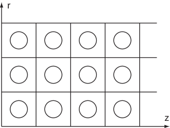
Figure 5.1. $(\psi_{z},\psi_{r})$ has $k$ vortices in $r$-direction.

Figure 5.2. The stable structure with a perturbation in space $H/(\Gamma\bigcup\tilde{H}).$

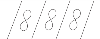
Figure 5.3. The stable structure with a perturbation in space $\tilde{H}\setminus\Gamma$.

6. Proof of Main Theorems

6.1. Proof of Theorem 3.1

We shall prove this theorem in the following several steps.

Step 1. We claim that the problem (3.1)-(3.3) bifurcates from $(u,\lambda)=(0,\lambda_{0})$ to a circle $S^{1}$ which consists of stead states.

It is easy to see that the problem (3.1) with (3.2) is invariant for the transition in the $z$-direction

$$u(z,r,t)\rightarrow u(z+z_{0},r,t)\qquad\text{ for}z_{0}\in\mathbb{R}^{1}.$$

Therefore, if $u_{0}$ is a steady state solution of (3.1) with (3.2), then for any $z_{0}\in\mathbb{R}^{1}$ the function $u_{0}(z+z_{0},r)$ is also a steady state solution. We can see that the set

$$\Sigma=\{u_{0}(z+z_{0},r)|\ z_{0}\in\mathbb{R}^{1}\}$$

is homeomorphic to a circle $S^{1}$ in $H_{1}$ for any $u_{0}\in H_{1}$. Hence, the singular points of (3.1) with (3.2) appear as a circle.

It is known in [16, 15] that there exist singular points bifurcated from $(u,\lambda)=(0,\lambda_{0})$. Thus this claim is proved.

Step 2. Reduction to the center manifold. We shall use the construction of center manifold functions to derive the reduced equations of (3.6) given by

(6.1) $$\left.\begin{aligned} &\frac{dx}{dt}=\beta_{1}(\lambda)x+\frac{(G(u),\psi^{*}_{1\lambda})_{H}}{(\psi_{1\lambda},\psi^{*}_{1\lambda})_{H}},\\ &\frac{dy}{dt}=\beta_{1}(\lambda)y+\frac{(G(u),\tilde{\psi}^{*}_{1\lambda})_{H}}{(\tilde{\psi}_{1\lambda},\tilde{\psi}^{*}_{1\lambda})_{H}},\end{aligned}\right.$$

where $\psi_{1\lambda}$ and $\tilde{\psi}_{1\lambda}$ are the eigenvectors of (3.10) corresponding to $\beta_{1}(\lambda)$ near $\lambda=\lambda_{0}$ with

(6.2) $$\left.\begin{aligned} &\lim_{\lambda\rightarrow\lambda_{0}}\psi_{1\lambda}=\psi_{1}&&(\psi_{1}\ \text{as\ in}\ (\ref{9.158})),\\ &\lim_{\lambda\rightarrow\lambda_{0}}\tilde{\lambda}_{1\lambda}=\tilde{\psi}_{1}&&(\tilde{\psi}_{1}\ \text{as\ in}\ (\ref{9.159})),\end{aligned}\right.$$

and $\psi^{*}_{1\lambda}$ and $\tilde{\psi}^{*}_{1\lambda}$ are the dual eigenvectors of $\psi_{1\lambda}$ and $\tilde{\psi}_{1\lambda}$ satisfying

(6.3) $$\left.\begin{aligned} &\lim\limits_{\lambda\rightarrow\lambda_{0}}\psi^{*}_{1\lambda}=\psi^{*}_{1}&&(\psi^{*}_{1}\ \text{as\ in}\ (\ref{9.161})),\\ &\lim\limits_{\lambda\rightarrow\lambda_{0}}\tilde{\psi}^{*}_{1\lambda}=\tilde{\psi}^{*}_{1}&&(\tilde{\psi}_{1}\ \text{as\ in}\ (\ref{9.162})).\end{aligned}\right.$$

Let $\Psi:E_{0}\rightarrow E^{\bot}_{0}$ be the center manifold function of (3.6) at $\lambda=\lambda_{0}$, where

$$E_{0}=\text{span}\{\psi_{1},\tilde{\psi}_{1}\},$$

$$E^{\bot}_{0}=\{u\in H|\ (u,\psi^{*}_{1})_{H}=0,(u,\tilde{\psi}^{*}_{1})_{H}=0\}.$$

Let $u_{0}=x\psi_{1}+y\tilde{\psi}_{1}\in E_{0}$. Then it is easy to check that $G(u_{0})\in E^{\bot}_{0}$. Hence, by the center manifold approximation formula in [12, 11], we find that

(6.4) $$\left.\begin{aligned} &\Psi=\phi(x,y)+o(|x|^{2}+|y|^{2})+O(\beta_{1}(\lambda)(|x|^{2}+|y|^{2})),\\ &-L_{\lambda}\phi=G(\psi_{1},\psi_{1})x^{2}+G(\tilde{\psi}_{1},\tilde{\psi}_{1})y^{2}+(G(\psi_{1},\tilde{\psi}_{1})+G(\tilde{\psi}_{1},\psi_{1}))xy.\end{aligned}\right.$$

On the center manifold, $u=u_{0}+\Phi(u_{0})$. Therefore from (6.1)-(6.4) we obtain the reduced equations of (3.6) to the center manifold as follows:

(6.5) $$\left.\begin{aligned} \frac{dx}{dt}=&\beta_{1}(\lambda)x+\frac{x}{\rho}(G(\phi,\psi_{1})+G(\psi_{1},\phi),\psi^{*}_{1})_{H}\\ &+\frac{y}{\rho}(G(\phi,\tilde{\psi}_{1})+G(\tilde{\psi}_{1},\phi),\psi^{*}_{1})_{H}\\ &+o(|x|^{3}+|y|^{3})+\varepsilon_{1}(\lambda)O(|x|^{3}+|y|^{3}),\\ \frac{dy}{dt}=&\beta_{1}(\lambda)y+\frac{x}{\rho}(G(\phi,\psi_{1})+G(\psi_{1},\phi),\tilde{\psi}^{*}_{1})_{H}\\ &+\frac{y}{\rho}(G(\phi,\tilde{\psi}_{1})+G(\tilde{\psi}_{1},\phi),\tilde{\psi}^{*}_{1})_{H}\\ &+o(|x|^{3}+|y|^{3})+\varepsilon_{2}(\lambda)O(|x|^{3}+|y|^{3}),\end{aligned}\right.$$

where $\rho=(\psi_{1},\psi^{*}_{1})_{H}=(\tilde{\psi}_{1},\tilde{\psi}^{*}_{1})_{H}$, and

$$\lim_{\lambda\to\lambda_{0}}\varepsilon_{i}(\lambda)=0\qquad(i=1,2).$$

Furthermore, direct calculation shows that

$$G(\psi_{1},\psi_{1})=P\psi_{0}+P\psi_{2}, G(\tilde{\psi}_{1},\tilde{\psi}_{1})=P\psi_{0}-P\psi_{2},$$

$$G(\psi_{1},\tilde{\psi}_{1})=P\tilde{\psi}_{0}+P\tilde{\psi}_{2}, G(\tilde{\psi}_{1},\psi_{1})=-P\tilde{\psi}_{0}+P\tilde{\psi}_{2}.$$

where $P:L^{2}(M)^{3}\rightarrow H$ is the Leray projection, and

$$\psi_{0}=-\left\{\begin{aligned} &0,\\ &\frac{1}{2}(a^{2}hD_{*}h+a^{2}hDh-\frac{1}{r}\varphi^{2}),\\ &\frac{a}{2}(\varphi D_{*}h+hD\varphi+\frac{1}{r}h\varphi),\end{aligned}\right.$$

$$\psi_{2}=-\left\{\begin{aligned} &\frac{a}{2}\sin 2az((D_{*}h)^{2}-hDD_{*}h),\\ &\frac{1}{2}\cos 2az(a^{2}hDh-a^{2}hD_{*}h-\frac{1}{r}\varphi^{2}),\\ &\frac{a}{2}\cos 2az(hD\varphi-\varphi D_{*}h+\frac{1}{r}\varphi h),\end{aligned}\right.$$

$$\tilde{\psi}_{0}=-\left\{\begin{aligned} &\frac{a}{2}((D_{*}h)^{2}+hDD_{*}h),\\ &0,\\ &0,\end{aligned}\right.$$

$$\tilde{\psi}_{2}=-\left\{\begin{aligned} &-\frac{a}{2}\cos 2az((D_{*}h)^{2}-hDD_{*}h),\\ &\frac{1}{2}\sin 2az(a^{2}hDh-a^{2}hD_{*}h-\frac{1}{r}\varphi^{2}),\\ &\frac{a}{2}\sin 2az(hD\varphi-\varphi D_{*}h+\frac{1}{r}\varphi h).\end{aligned}\right.$$

Thus, (6.4) is rewritten as

(6.6) $$(A-\lambda_{0}B)\phi=(x^{2}+y^{2})P\psi_{0}+(x^{2}-y^{2})P\psi_{2}+2xyP\tilde{\psi}_{2}.$$

Let

(6.7) $$\phi=-[(x^{2}+y^{2})\phi_{0}+(x^{2}-y^{2})\phi_{2}+2xy\tilde{\phi}_{2}],$$

(6.8) $$\left\{\begin{aligned} &\phi_{0}=(0,0,\varphi_{0}),\\ &\phi_{2}=(-1/2\sin 2az\varphi_{z},\cos 2az\varphi_{r},\cos 2az\varphi_{\theta}),\\ &\tilde{\phi}_{2}=(1/2\cos 2az\tilde{\phi}_{z},\sin 2az\tilde{\phi}_{r},\sin 2az\tilde{\phi}_{\theta}).\end{aligned}\right.$$

Then we deduce from (6.6) and (6.7) that

$$\varphi_{z}=\tilde{\varphi}_{z},\ \ \ \ \varphi_{r}=\tilde{\varphi}_{r},\ \ \ \ \varphi_{\theta}=\tilde{\varphi}_{\theta},$$

and $(\varphi_{z},\varphi_{r},\varphi_{\theta})$ satisfies

$$(DD_{*}-4a^{2})\varphi_{r}+4a^{2}\lambda_{0}(\frac{1}{r^{2}}-\kappa)\varphi_{\theta}=4a^{2}H_{2}+2aDH_{1},$$

$$(DD_{*}-4a^{2})\varphi_{\theta}+\lambda_{0}\kappa\varphi_{r}=H_{3},$$

$$\varphi_{z}=\frac{1}{2a}D_{*}\varphi_{r},$$

$$\varphi_{z}=0,\varphi_{\theta}=0,\varphi_{r}=D\varphi_{r}=0\ \ \ \ \text{at}\ \ \ \ r=\eta,1,$$

where $H_{1},H_{2}$, and $H_{3}$ are given by

(6.9) $$\left.\begin{aligned} &H_{1}=a((D_{*}h)^{2}-hDD_{*}h),\\ &H_{2}=a^{2}hDh-a^{2}hD_{*}h-\frac{1}{r}\varphi^{2},\\ &H_{3}=a(hD\varphi-\varphi D_{*}h+\frac{1}{r}\varphi h).\end{aligned}\right.$$

Based on (6.8) we find

$$(G(\tilde{\psi}_{1},\phi_{i})+G(\phi_{i},\tilde{\psi}_{1}),\psi^{*}_{1})_{H}=0\ \ \ \ \text{for}\ \ \ \ i=0,2,$$

$$(G(\psi_{1},\phi_{i})+G(\phi_{i},\psi_{1}),\tilde{\psi}^{*}_{1})_{H}=0\ \ \ \ \text{for}\ \ \ \ i=0,2,$$

$$(G(\tilde{\psi}_{1},\tilde{\phi}_{2})+G(\tilde{\phi}_{2},\tilde{\psi}_{1}),\tilde{\psi}^{*}_{1})_{H}=0,$$

$$(G(\psi_{1},\tilde{\phi}_{2})+G(\tilde{\phi}_{2},\psi_{1}),\psi^{*}_{1})_{H}=0.$$

Then, putting (6.7) into (6.5), we deduce that

(6.10) $$\left.\begin{aligned} \frac{dx}{dt}=\beta_{1}x&-\frac{1}{\rho}x(x^{2}+y^{2})(G(\phi_{0},\psi_{1})+G(\psi_{1},\phi_{0}),\psi^{*}_{1})_{H}\\ &-\frac{1}{\rho}x(x^{2}-y^{2})(G(\phi_{2},\psi_{1})+G(\psi_{1},\phi_{2}),\psi^{*}_{1})_{H}\\ &-\frac{2}{\rho}xy^{2}(G(\tilde{\phi}_{2},\tilde{\psi}_{1})+G(\tilde{\psi}_{1},\tilde{\phi}_{2}),\psi^{*}_{1})_{H}\\ &+o(|x|^{3}+|y|^{3})+\varepsilon_{1}(\lambda)O(|x|^{3}+|y|^{3}),\\ \frac{dy}{dt}=\beta_{1}y&-\frac{1}{\rho}y(x^{2}+y^{2})(G(\phi_{0},\tilde{\psi}_{1})+G(\tilde{\psi}_{1},\phi_{0}),\tilde{\psi}^{*}_{1})_{H}\\ &-\frac{1}{\rho}y(x^{2}-y^{2})(G(\phi_{2},\tilde{\psi}_{1})+G(\tilde{\psi}_{1},\phi_{2}),\tilde{\psi}^{*}_{1})_{h}\\ &-\frac{2}{\rho}yx^{2}(G(\tilde{\phi}_{2},\psi_{1})+G(\psi_{1},\tilde{\phi}_{2}),\tilde{\psi}^{*}_{1})_{H}\\ &+o(|x|^{2}+|y|^{2})+\varepsilon_{2}(\lambda)O(|x|^{3}+|y|^{3}).\end{aligned}\right.$$

Direct computation yields

$$(G(\phi_{2},\psi_{1})+G(\psi_{1},\phi_{2}),\psi^{*}_{1})_{H} = (G(\tilde{\phi}_{2},\tilde{\psi}_{1})+G(\tilde{\psi}_{1},\tilde{\phi}_{2}),\psi^{*}_{1})_{H}$$

$$= (G(\phi_{2},\tilde{\psi}_{1})+G(\tilde{\psi}_{1},\phi_{2}),\tilde{\psi}^{*}_{1})_{H}$$

$$= (G(\tilde{\phi}_{2},\psi_{1})+G(\psi_{1},\tilde{\phi}_{2}),\tilde{\psi}^{*}_{1})_{H}.$$

Hence (6.10) can be rewritten as

(6.11) $$\left.\begin{aligned} &\frac{dx}{dt}=\beta_{1}x+Rx(x^{2}+y^{2})+o(|x|^{3}+|y|^{3})+\varepsilon_{1}(\lambda)O(|x|^{3}+|y|^{3}),\\ &\frac{dy}{dt}=\beta_{1}y+Ry(x^{2}+y^{2})+o(|x|^{3}+|y|^{3})+\varepsilon_{2}(\lambda)O(|x|^{3}+|y|^{3}),\end{aligned}\right.$$

where

(6.12) $$R=-\frac{1}{\rho}(G(\phi_{0}+\phi_{2},\psi_{1})+G(\psi_{1},\phi_{2}+\phi_{2}),\psi^{*}_{1})_{H}.$$

On the other hand, we infer from (6.6) and (6.8) that

$$(A-\lambda_{0}B)\phi_{i}=P\psi_{i}\qquad\text{ for }i=0,2,$$

Hence we find

$$\left.\begin{aligned} &\Phi=-(\phi_{0}+\phi_{2}),\\ &(A-\lambda_{0}B)\Phi=G(\psi_{1},\psi_{1})=P\psi_{0}+P\psi_{2}.\end{aligned}\right.$$

Thus the number (6.12) is the same as that in (3.24).

Step 3. Proof of Assertions (1)-(4). When $R<0$, $(x,y)=0$ is locally asymptotically stable for (6.11) at $\lambda=\lambda_{0}$. Therefore $u=0$ is a locally asymptotically stable singular point of (3.6). By the attractor bifurcation theorem, Theorem 6.1 in p. 153 in [5], the problem (3.1)-(3.3) bifurcates from $(u,\lambda)=(0,\lambda_{0})$ to an attractor ${\mathcal{A}}_{\lambda}$ which attracts an open set $U\setminus\Gamma$, and Assertions (1), (3) and (4) hold true.

In addition, the nonlinear terms in (6.11) satisfy the coercive condition in the $S^{1}$-attractor bifurcation theorem (Theorem 5.10 in [5]) and the conclusion in Step 1., and Assertion (2) follows.

Step 4. Attraction in $C^{r}$-norm. It is known that for any initial value $u_{0}\in H$ there is a time $t_{0}>0$ such that the solution $u(t,u_{0})$ of (3.1)-(3.3) is analytic for $t>t_{0}$, and uniformly bounded in $C^{r}$-norm for any $r\geq 1$; see Theorem 1 in [7]. Hence, by Assertion (4), for any $u_{0}\in U\setminus\Gamma$ we have

(6.13) $$\lim\limits_{t\rightarrow\infty}\min\limits_{v_{0}\in{\mathcal{A}}_{\lambda}}\|u(t,u_{0})-v_{0}\|_{C^{r}}=0.$$

Step 5. Structure of solutions in ${\mathcal{A}}_{\lambda}$. By Assertion (3), for any steady state solution $u_{0}=(u_{z},u_{r},u_{\theta})\in{\mathcal{A}}_{\lambda}$, the vector field $\tilde{u}=(u_{z},u_{r})$ of $u_{0}$ can be expressed as

(6.14) $$\left.\begin{aligned} &u_{z}=\gamma\cos a(z+z_{0})D_{*}h(r)+w_{1}(z,r,\beta_{1}),\\ &u_{r}=a\gamma\sin a(z+z_{0})h(r)+w_{2}(z,r,\beta_{1}),\end{aligned}\right.$$

for some $z_{0}\in\mathbb{R}^{1}$, where

$$\gamma=|\beta_{1}(\lambda)/R|^{1/2},\qquad w_{i}=o(|\beta_{1}|^{1/2})\qquad\text{ for }i=1,2.$$

As in the proof of Theorem 4.1 in [8], we deduce that the vector field (6.14) is $D$-regular for all $0<\lambda-\lambda_{0}<\varepsilon$ for some $\varepsilon>0$. Moreover, the first order vector field in (6.14)

(6.15) $$(v_{z},v_{r})=(\gamma\cos a(z+z_{0})D_{*}h(r),a\gamma\sin a(z+z_{0})h(r))$$

has the topological structure as shown in Figure 3.2.

Furthermore, it is easy to check that the space

$$\tilde{H}=\left\{u=(u_{z},u_{r},u_{\theta})\in H|\ \int_{M}ru_{z}drdz=0\right\}$$

is invariant for the operator $L_{\lambda}+G$ defined by (3.5). To see this, since $u$ is $z$-periodic and $u=0$ at $r=1,\eta$, we have

$$\int^{L}_{0}\int^{1}_{\eta}r(\tilde{u}\cdot\nabla)u_{z}drdz = \int^{L}_{0}\int^{1}_{\eta}ru_{r}\frac{\partial u_{z}}{\partial r}drdz$$

$$= -\int^{L}_{0}\int^{1}_{\eta}\frac{\partial(ru_{r})}{\partial r}u_{z}drdz$$

$$= \int^{L}_{0}\int^{1}_{\eta}r\frac{\partial u_{z}}{\partial z}u_{z}drdz$$

$$= 0\qquad\forall u\in H,$$

$$\int^{L}_{0}\int^{1}_{\eta}r\Delta u_{z}drdz=0,\ \ \ \ \forall u\in\tilde{H}.$$

Thus we see that $\tilde{H}$ is invariant for $L_{\lambda}+G$.

Therefore, for the vector field (6.13) we have

$$\int_{M}ru_{z}drdz=0.$$

By The Connection Lemma and the orbit-breaking method in [6], it implies that the vector field (6.14) is topologically equivalent to its first order field (6.15) for $0<\lambda-\lambda_{0}<\varepsilon$.

Step 6. Proof of Assertions (5) and (6). For any initial value $u_{0}\in U\setminus(\Gamma\bigcup\tilde{H})$, we have

(6.16) $$u_{0}=\sum_{k=1}^{\infty}\alpha_{k}e_{k}+w_{0},$$

where $w_{0}\in\tilde{H}$, and for any $k=1,2,\cdots,$

$$e_{k}=(\tilde{e}_{k}(r),0,0),$$

$$\int^{1}_{\eta}\tilde{e}_{k}(r)dr\neq 0,$$

and $\tilde{e}_{k}(r)$ satisfies that

$$\left.\begin{aligned} &D_{*}D\tilde{e}_{k}=-\rho_{k}\tilde{e}_{k},\\ &\tilde{e}_{k}|_{r=\eta,1}=0,\\ &0<\rho_{1}<\rho_{2}<\cdots.\end{aligned}\right.$$

Make the decomposition

$$H_{1}=E\bigoplus\tilde{H}_{1}\ \ \ \ (\tilde{H}_{1}=H_{1}\bigcap\tilde{H}),$$

$$H=E\bigoplus\tilde{H},$$

$$E=\text{span}\{e_{1},e_{2},\cdots\}.$$

Then the equation (3.6) can be decomposed into

(6.17) $$\left.\begin{aligned} &\frac{de}{dt}=L_{\lambda}e&&e\in E,\\ &\frac{dw}{dt}=L_{\lambda}w+G(w)&&w\in\tilde{H}_{1},\\ &(e(0),w(0))=(\sum_{k}\alpha_{k}e_{k},w_{0}).\end{aligned}\right.$$

It is obvious that

$$L_{\lambda}e_{k}=-\rho_{k}e_{k}.$$

Hence for the initial value (6.16), the solution $u(t,u_{0})$ of (6.17) can be expressed as

(6.18) $$\left.\begin{aligned} &u(t,u_{0})=\sum\limits_{k}\alpha_{k}e^{-\rho_{k}t}e_{k}+w(t,u_{0}),\\ &\int^{1}_{\eta}e_{k}(r)dr\neq 0.\end{aligned}\right.$$

By (6.13) we have

$$\lim_{t\to\infty}\|w(t,u_{0})-v_{0}\|_{C^{r}}=0,\qquad v_{0}\in{\mathcal{A}}_{\lambda},$$

which implies by Step 5 that $w(t,u_{0})$ is topologically equivalent to (6.15) for $t>0$ sufficiently large, i.e., $w(t,u_{0})$ has the topological structure as shown in Figure 3.2.

By the structural stability theorem, Theorem 2.2.9 and Lemmas 2.3.1 and 2.3.3 (connection lemmas) in [6], we infer from (6.18) that the vector field in (6.18) is topologically equivalent to either the structure as shown in Figure 3.1(a) or the structure as shown in 3.1(b), dictated by the sign of $\alpha_{k_{0}}$ in (6.16) with $k_{0}=\min\{k|\alpha_{k}\neq 0\}$. Thus Assertion (5) is proved.

Assertion (6) can be derived by the invariance of $\tilde{H}$ under the operator $L_{\lambda}+G$ and the structural stability theorem with perturbation in $\tilde{H}$, in the same fashion as in the proof of Theorem 2.2.9 in [6] by using the Connection Lemma.

The proof of Theorem 3.1 is complete.

6.2. Proof of Theorem 3.2

When $R>0$, by Theorem A.2 in [10], we infer from the reduced equation (6.11) that the transition of (3.1)-(3.3) is of Type-II. In the following, we shall use the saddle-node bifurcation theorem, Theorem A.7 in [10], to prove this theorem. Let

$$H^{*}=\{(u_{z},u_{r},u_{\theta})\in H|\ u_{z}(-z,r)=-u_{z}(z,r)\},$$

$$H^{*}_{1}=H_{1}\bigcap H^{*}.$$

It is easy to see that the space $H^{*}$ is invariant under the action of the operator $L_{\lambda}+G$ defined by (3.5):

(6.19) $$L_{\lambda}+G:H^{*}_{1}\rightarrow H^{*},$$

and the first eigenvalue $\beta_{1}(\lambda)$ of $L_{\lambda}:H^{*}_{1}\rightarrow H^{*}$ at $\lambda=\lambda_{0}(T=T_{c})$ is simple, with the first eigenvector $\psi_{1}$ given by (3.15). Hence, the number $R$ in (6.12) is valid for the mapping (6.18), i.e.,

$$(G(x\psi_{1}+\Phi(x),\psi^{*}_{1})=Rx^{3}+o(|x|^{3}).$$

Thus, it is readily to check that all conditions in Theorem A.7 in [10] are fulfilled by the operator (6.19). By Step 1 in the proof of Theorem 3.1, each singular point of (6.19) generates a singularity circle for $L_{\lambda}+G$ in $H$. Therefore, Theorem 3.2 follows from Theorem A.7 in [10].

The proof of Theorem 3.2 is complete.

References

- [1] S. Chandrasekhar, Hydrodynamic and Hydromagnetic Stability, Dover Publications, Inc., 1981.
- [2] P. Drazin and W. Reid, Hydrodynamic Stability, Cambridge University Press, 1981.
- [3] K. Kirchgässner, Bifurcation in nonlinear hydrodynamic stability, SIAM Rev., 17 (1975), pp. 652–683.
- [4] T. Ma and S. Wang, Structural evolution of the Taylor vortices, M2AN Math. Model. Numer. Anal., 34 (2000), pp. 419–437. Special issue for R. Temam’s 60th birthday.
- [5] , Bifurcation theory and applications, vol. 53 of World Scientific Series on Nonlinear Science. Series A: Monographs and Treatises, World Scientific Publishing Co. Pte. Ltd., Hackensack, NJ, 2005.
- [6] , Geometric theory of incompressible flows with applications to fluid dynamics, vol. 119 of Mathematical Surveys and Monographs, American Mathematical Society, Providence, RI, 2005.
- [7] , Stability and bifurcation of the Taylor problem, Arch. Ration. Mech. Anal., 181 (2006), pp. 149–176.
- [8] , Rayleigh-Bénard convection: dynamics and structure in the physical space, Commun. Math. Sci., 5 (2007), pp. 553–574.
- [9] , Exchange of stabilities and dynamic transitions, Georgian Mathematics Journal, 15:3 (2008), pp. 581–590.
- [10] , Cahn-hilliard equations and phase transition dynamics for binary systems, Dist. Cont. Dyn. Systs., Ser. B, 11:3 (2009), pp. 741–784.
- [11] , Phase Transition Dynamics in Nonlinear Sciences, submitted, 2009.
- [12] , Dynamic transition theory for thermohaline circulation, Physica D, 239:3-4 (2010), pp. 167–189.
- [13] G. I. Taylor, Stability of a viscous liquid contained between two rotating cylinders, Philos. Trans. Royl London Ser. A, 223 (1923), pp. 289–243.
- [14] R. Temam, Navier-Stokes Equations, Theory and Numerical Analysis, 3rd, rev. ed., North Holland, Amsterdam, 1984.
- [15] W. Velte, Stabilität and verzweigung stationärer lösungen der davier-stokeschen gleichungen, Arch. Rat. Mech. Anal., 22 (1966), pp. 1–14.
- [16] V. I. Yudovich, Secondary flows and fluid instability between rotating cylinders, . Appl. Math. Mech., 30 (1966), pp. 822–833.