AEI-2010-092

Matrix factorisations describe B-type boundary conditions in $\mathcal{N}=2$ supersymmetric Landau-Ginzburg models. At the infrared fixed point, they correspond to superconformal boundary states. We investigate the relation between boundary states and matrix factorisations in the Grassmannian Kazama-Suzuki coset models. For the first non-minimal series, i.e. for the models of type $SU(3)_{k}/U(2)$, we identify matrix factorisations for a subset of the maximally symmetric boundary states. This set provides a basis for the RR charge lattice, and can be used to generate (presumably all) other boundary states by tachyon condensation.

1 Introduction

In this article we want to study the relation between two different and complementary descriptions of B-type boundary conditions in $\mathcal{N}=(2,2)$ supersymmetric two-dimensional field theories: the description in terms of matrix factorisations of a superpotential, and the description in terms of boundary states. Such field theories arise as world-sheet theories of open strings which end on B-type D-branes. To motivate our investigation let us look at the moduli space of string theory compactified on a six-dimensional Calabi-Yau manifold. This moduli space is in general very complicated and consists of different phases [1]. In a large volume regime we have a description in terms of a non-linear sigma-model on the background geometry, and we can use geometric tools. At some other region of the moduli space we might have a description in terms of Landau-Ginzburg models governed by some holomorphic superpotential $W$. At special points of the moduli space, the superconformal field theory that is described by the Landau-Ginzburg model is in fact a rational conformal field theory (CFT), which means that it has a large chiral symmetry algebra that turns the theory solvable. A typical example is the Gepner point in moduli space.

When we discuss D-branes in such backgrounds, a natural question to ask is how they behave when the closed string moduli are deformed. We shall focus in this paper on B-type D-branes. In the aforementioned regimes, one has different descriptions for the branes. In the geometric regime they are described by holomorphic submanifolds, or more generally by complexes of coherent sheaves (see e.g. [2]). In the Landau-Ginzburg models the B-type boundary conditions are described by factorisations of the superpotential in terms of matrices (see e.g. [3]). The connection between these descriptions has been clarified in [4] using gauged linear sigma models as a description in the whole moduli space.

It is less clear how to connect the description in terms of matrix factorisations to the formulation of B-type boundary conditions at the points where we have a rational conformal field theory description. Such a connection would be desirable to have, because both descriptions have their advantages. Matrix factorisations easily allow to discuss the dependence on the moduli, whereas the rational CFT description is only available at one point. On the other hand, in the Landau-Ginzburg formulation, one can only access few data directly, namely topological data such as RR charges, but not e.g. the mass of the brane, whereas in the rational CFT we know the couplings of all fields to the brane.

We are looking for some dictionary between matrix factorisations and rational boundary states, not only for the case of Calabi-Yau backgrounds, but for the general situation where a supersymmetric rational CFT admits a Landau-Ginzburg description. Setting up such a dictionary is a highly non-trivial problem. To get from the Landau-Ginzburg formulation to the CFT description one has to follow a renormalisation group flow to the infrared, but these flows are usually not under good control. Only some ’topological’ data is protected under renormalisation.

The other problem we have to face is that on the CFT side, our tools only allow us to construct rational boundary states, i.e. boundary states which preserve the chiral symmetry algebra. In general, this will only be a subset of all superconformal boundary states. Therefore we should not expect to find a simple prescription of how to obtain a boundary state from any matrix factorisation. More realistically, one can hope to find answers to the following two questions: Can we determine a matrix factorisation from a given boundary state? Can we understand on the matrix factorisation side what distinguishes the ’rational’ boundary conditions from the rest?

One approach to these questions is to study the relation of matrix factorisations and rational boundary states in a large class of models, and to look for general patterns. Up to now, most comparisons have been performed in minimal models [5, 6, 7, 8]. Minimal models are very special in the sense that we only have a finite number of elementary boundary states and matrix factorisations that have to be matched. Also products of minimal models have been considered [9, 10]. Here one encounters for the first time the situation that the rational boundary states only present a subset of all boundary states.

A more general class of rational $\mathcal{N}=(2,2)$ supersymmetric rational CFTs is provided by the Kazama-Suzuki models [11], which are based on a coset construction $G/H$. Not all of these models, however, have a description as a Landau-Ginzburg theory. A subclass with this property is given by those models where the group $G$ is simply laced, the corresponding level is $1$, and $G/H$ is a Hermitian symmetric space [12]. A two-parameter family of such models is given by the Grassmannian cosets, where $G=SU(n+k)$ and $H=S(U(n)\times U(k))$. For $n=1$ one recovers the minimal models. The first non-minimal family of Grassmannian models is given by $n=2$. For these models we want to extend the connection between the coset and the Landau-Ginzburg description to the case when B-type boundary conditions are present.

In the Grassmannian models $SU(3)_{k}/U(2)$, we explicitly identify the matrix factorisations that correspond to a set of B-type boundary states that form a basis of the Ramond-Ramond charge lattice. To do the identifications between matrix factorisations and boundary states we compare the open string spectra, the RR charges and also information on boundary renormalisation group flows. We expect to find all other boundary states and matrix factorisations from tachyon condensation of the basic ones. We illustrate and confirm this idea, and construct matrix factorisations that correspond to another subset of boundary states. For low levels ($k=1,2$), this means that we can identify matrix factorisations for all rational boundary states, for higher levels we believe that by performing more tachyon condensations we would eventually identify all remaining factorisations.

The paper is organised as follows: In section 2 we shall discuss the Grassmannian Kazama-Suzuki models, in particular their field content and their B-type boundary states. For the model $SU(3)/U(2)$ we then go more into detail and evaluate the spectra of the boundary theories and the RR charges. In section 3 the Landau-Ginzburg description is introduced. First we review the identification of the superpotential that corresponds to the Grassmannian cosets, then we study factorisations of the superpotentials for the $SU(3)/U(2)$ series. A number of basic factorisations is given and the corresponding RR charges are determined. Section 4 then deals with the comparison between CFT and LG description. By analysing spectra and RR charges, it is shown how to identify some of the boundary states with matrix factorisations. We then discuss boundary renormalisation group flows and tachyon condensation. On the one hand, we can use these to compare the CFT and LG description, on the other hand we can use them to find factorisations for the remaining boundary states. This is exemplified for another family of boundary states. For low levels, where our models are equivalent to minimal models, we compare in section 5 our findings to results in the literature. In the concluding section 6 we discuss some open problems and possible routes to solve them. Two appendices contain the details of the calculations that form the basis of our identifications between CFT and LG description.

2 Kazama-Suzuki models

Kazama and Suzuki [14, 11] constructed a large class of rational CFTs with $\mathcal{N}=2$ superconformal symmetry as coset models of the form

$$\frac{G_{k}\times SO(2d)_{1}}{H}\ .$$ (2.1)

Here, $G$ is a simple, compact Lie group, $k$ the corresponding level, $2d$ is the difference of the dimensions of $G$ and of the regularly embedded subgroup $H$ (which we take to have the same rank as $G$). To have $\mathcal{N}=2$ supersymmetry, $G/H$ has to be Kähler and hence the difference of dimensions, $2d$, is even.

Of particular interest are the models where $G$ is simply laced, the level is $k=1$, and $G/H$ is a Hermitian symmetric space. In this case, the CFTs have a description as Landau-Ginzburg models [12]. These theories have been classified [11], and a prominent family of such models is provided by the Grassmannians, where $G=SU(n+k)$ and $H=S(U(n)\times U(k))$.

2.1 Grassmannians: the bulk theory

The Grassmannian cosets are of the form

$$\frac{SU(n+k)_{1}\times SO(2nk)_{1}}{SU(n)_{k+1}\times SU(k)_{n+1}\times U(1)}\cong\frac{SU(n+1)_{k}\times SO(2n)_{1}}{SU(n)_{k+1}\times U(1)}\ .$$ (2.2)

with central charge $c=\frac{3nk}{k+n+1}$. The equivalence used here is known as level-rank duality [11, 12, 15, 16, 17, 18, 19, 20].

We shall most of the time work in the formulation on the right hand side. The ’embedding’ homomorphism of the denominator group into the numerator group is

$$i(h,\zeta)=\begin{pmatrix}h\zeta&0\\ 0&\zeta^{-n}\end{pmatrix}\in SU(n+1)\ ,$$ (2.3)

where $h\in SU(n)$ is a $n\times n$-matrix, and $\zeta\in U(1)$ is a phase. Note that this is not a one-to-one mapping, because $i(\xi^{-1}\mathbf{1},\xi)=\mathbf{1}$ for $\xi^{n}=1$. This just means that the denominator group only becomes a subgroup of the numerator group after taking a $\mathbb{Z}_{n}$ quotient,

$$U(n)=\big{(}SU(n)\times U(1)\big{)}/\mathbb{Z}_{n}\ .$$ (2.4)

This will become important shortly when we discuss selection and identification rules.

The sectors of the theory are labelled by quadruples $(\Lambda,\Sigma;\lambda,\mu)$, where $\Lambda$ is a dominant weight of $su(n+1)_{k}$, $\lambda$ is a dominant weight of $su(n)_{k+1}$, $\mu$ is an integer labelling a $u(1)$-representation, and finally $\Sigma$ labels a dominant weight of $so(2n)_{1}$, so it labels either the trivial representation $0$, the vector ($v$), the spinor ($s$) or the anti-spinor $(\bar{s})$ representation. Representations with $\Sigma=0,v$ belong to the Neveu-Schwarz sector, $\Sigma=s,\bar{s}$ belong to the Ramond sector.

As usual, the representation labels are restricted by selection rules, and we have an equivalence relation on the allowed labels given by identification rules [12, 21, 22]. The appearance of selection and identification rules is connected to the existence of a non-trivial common center $Z$ of the numerator and denominator theory, or better the preimage $Z=i^{-1}(Z_{G})$ of the center of the numerator group $G=SU(n+1)$. Here, $Z_{SU(n+1)}=\{\eta\mathbf{1}|\eta^{n+1}=1\}$, so that $Z=\{(\xi^{-1}\mathbf{1},\xi\eta)|\xi^{n}=1,\eta^{n+1}=1\}$. This is a cyclic group $\mathbb{Z}_{n(n+1)}$ with generator $(e^{-2\pi i/n}\mathbf{1},e^{2\pi i/n}e^{2\pi i/(n+1)})$.

Corresponding to the center $Z$, there is a cyclic simple current group $G_{\text{id}}$ that acts on the weights [23, 24]. It is generated by the simple current $J_{0}=(J_{n+1},v;J_{n},k+n)$, where $J_{n+1}=k\omega_{1}$ generates the simple current group of $su(n+1)_{k}$, and $J_{n}=(k+1)\omega_{1}$ generates the simple current group of $su(n)_{k+1}$ (here, we denote for both $su(n)$ and $su(n+1)$ the first fundamental weight by $\omega_{1}$). In the $u(1)$-part, the simple current acts as $\mu\to\mu+k+n$. Since $J_{0}^{n(n+1)}$ should act as the identity, the $u(1)$ labels $\mu$ should be periodically identified with period $n(n+1)(k+n)$. This means that the $u(1)$ Heisenberg algebra can be enlarged to $u(1)_{n(n+1)(k+n)}$.

The simple current group $G_{\text{id}}$ acts without fixed-points on the quadruples of weights and generates the identification rules. On the other hand, the selection rules are encoded in the requirement that the monodromy charges of the numerator and denominator parts should be equal,

$$Q_{J_{n+1}}(\Lambda)+Q_{v}(\Sigma)\overset{!}{=}Q_{J_{n}}(\lambda)+Q_{k+n}(\mu)\ .$$ (2.5)

The monodromy charges are defined as usual as differences of conformal weights, $Q_{J}(\phi)=h_{J}+h_{\phi}-h_{J\phi}\mod 1$.

The sectors of the theory are labelled by equivalence classes $[\Lambda,\Sigma;\lambda,\mu]$ of allowed labels. An important subset of representations of the coset algebra is the set of chiral primary states. It can be shown [15] that in the Grassmannian models a chiral primary can be represented as

$$[\Lambda,0;P_{n}\Lambda,P_{U}\Lambda]\ .$$ (2.6)

Here $P_{n}$ and $P_{U}$ are the projection matrices that map $su(n+1)$ weights to $su(n)$ and $u(1)$ weights, respectively. In terms of Dynkin labels they are explicitly given as

$$P_{n}(\Lambda_{1},\dotsc,\Lambda_{n}) =(\Lambda_{1},\dotsc,\Lambda_{n-1}) P_{U}(\Lambda_{1},\dotsc,\Lambda_{n}) =\Lambda_{1}+2\Lambda_{2}+\dotsb+n\Lambda_{n}\ .$$ (2.7)

The above statement about the form of the chiral primaries makes it easy to obtain the number of chiral primary states – it is just given by the number of dominant highest weights of $su(n+1)_{k}$, i.e.

$$\text{number of chiral primaries}\ =\binom{k+n}{n}\ .$$ (2.8)

Up to now we have only discussed representation theoretic aspects. When we want to consider a conformal field theory (without boundaries for the moment), we have to specify the spectrum, which we shall take to be of (almost) diagonal form,

$$\mathcal{H}=\bigoplus_{[\Lambda,\Sigma;\lambda,\mu]}\mathcal{H}_{[\Lambda,\Sigma;\lambda,\mu]}\otimes\mathcal{H}_{[\Lambda,\Sigma^{+};\lambda,\mu]}\ .$$ (2.9)

Two comments are in order. The most natural thing would be to consider the charge conjugated spectrum. It turns out, however, that the diagonal spectrum is the one that is related to the Landau-Ginzburg models that we shall discuss later. Of course, we can use the mirror automorphism to map one spectrum into the other, but then we would also map B-type boundary conditions to A-type, and if we want to relate B-type conditions in the coset model to B-type in the Landau-Ginzburg theory, it is the diagonal spectrum that we have to choose. The other comment concerns the small deviation from the diagonal theory, namely the charge conjugation on the $so(2n)_{1}$ representation. This is the right choice to obtain the Landau-Ginzburg theories with the standard potentials that we introduce later. If we twist the spectrum by applying the outer automorphism that exchanges spinor and anti-spinor, we obtain the theory where we add a quadratic term $z^{2}$ to the superpotential.

2.2 Boundary conditions

We now want to discuss the theory on a world-sheet with a boundary, which we take to be the upper half plane. At the real axis, we impose B-type gluing conditions for the energy momentum tensor $T$, the current $J$ and the supercurrents $G^{\pm}$,

$$T(z) =\bar{T}(\bar{z}) J(z) =\bar{J}(\bar{z}) G^{\pm}(z) =\eta\bar{G}^{\pm}(\bar{z})$$ (2.10)

at $z=\bar{z}$. Here, $\eta$ is a sign corresponding to the choice of a spin structure. The sign of $\eta$ does of course not affect the gluing conditions for the fields of the bosonic subalgebra of the $\mathcal{N}=2$ superconformal algebra.

In general, the classification and construction of boundary states with the above gluing conditions is a difficult and unsolved problem. We need to restrict our focus on highly symmetric boundary conditions, which satisfy gluing conditions on more fields of our chiral symmetry algebra. Denoting by $W(z)$ any chiral field of the coset algebra, we can impose the gluing condition [27]

$$W(z)=\omega(\bar{W})(\bar{z})\quad\text{at}\ z=\bar{z}\ .$$ (2.11)

Here, $\omega$ is an automorphism of the coset algebra. The coset algebra contains the bosonic subalgebra of the $\mathcal{N}=2$ superconformal algebra, so the gluings we choose for the coset theory should be consistent with the B-type gluing conditions.

The classification of automorphisms of coset algebras is not known, but there is a particularly nice class of automorphisms that we can use. An automorphism of this class is induced by an automorphism $\omega_{G}$ of the group $G$ that can be restricted to an automorphism $\omega_{H}$ of $H$, in the sense that $i(\omega_{H}(h))=\omega_{G}(i(h))$ for all $h\in H$. In [26] the automorphisms of this type have been classified, and it is also analysed which automorphisms correspond to B-type gluing conditions. In the Grassmannian models, only the trivial automorphism is possible.

This, however, still means that we have to deal with twisted boundary conditions, because we chose a diagonal bulk spectrum which is twisted (by conjugation) with respect to the standard theory with charge conjugated spectrum. In particular this means that only those sectors of the bulk theory can couple to the branes which are invariant under charge conjugation.

Our discussion leads to the conclusion that only those bulk fields can couple to the boundary that belong to $\mathcal{H}_{[\Lambda,\Sigma;\lambda,\mu]}\otimes\mathcal{H}_{[\Lambda,\Sigma^{+};\lambda,\mu]}$ satisfying

$$[\Lambda,\Sigma;\lambda,\mu]=[\Lambda^{+},\Sigma;\lambda^{+},-\mu]\ .$$ (2.12)

Note that because of our choice of the spectrum, the $so(2n)_{1}$-label $\Sigma$ appears without conjugation on the right hand side.

To analyse the condition (2.12), we have to take into account that only the equivalence classes of labels have to agree. Let us denote the quadruples by $\alpha$ and the automorphism appearing on the right hand side of (2.12) by $C$. Solving $[\alpha]=[C(\alpha)]$ then means to find all equivalence classes $[\alpha]$ such that

$$\alpha=JC(\alpha)$$ (2.13)

for some simple current $J$ of the identification group $G_{\text{id}}$. If $\alpha$ is a solution to the above equation, then of course $J^{\prime}\alpha$ is also a solution, but possibly for a different $J$. In our case, commuting the charge conjugation with the action of a simple current just inverts the current, so that we get

$$J^{\prime}\alpha=J^{\prime}JC(\alpha)=J^{\prime}JJ^{\prime}C(J^{\prime}\alpha)\ .$$ (2.14)

Hence, $J^{\prime}\alpha$ satisfies (2.13) if $J$ is replaced by $J^{\prime}JJ^{\prime}$. In other words we only have to investigate (2.13) for one representative $J$ of each orbit $\mathcal{C}_{J}=\{J^{\prime}JJ^{\prime}|J^{\prime}\in G_{\text{id}}\}$. In our case where $G_{\text{id}}$ is just a cyclic group of even order, there are two orbits: one generated by $1$ (containing the even powers of $J_{0}$) and one generated by $J_{0}$ (consisting of the odd powers of $J_{0}$). So we are led to consider solutions to the condition

$$(\Lambda,\Sigma;\lambda,\mu)=(\Lambda^{+},\Sigma;\lambda^{+},-\mu)$$ (2.15)

and solutions of

$$(\Lambda,\Sigma;\lambda,\mu)=(J_{n+1}\Lambda^{+},v\Sigma;J_{n}\lambda^{+},-\mu+k+n)\ .$$ (2.16)

As is obvious from the condition on the $so(2n)_{1}$-label, the latter equation does not have a solution, so the only sectors that couple to the boundary correspond to solutions of the first condition. On the set of labels that satisfy this condition, we still have the action of a subgroup of the identification group; it is clear from the discussion above and (2.14) that apart from the identity only the element $J_{0}^{n(n+1)/2}$ maps this set to itself. We can use this identification to set the $U(1)$-label to $\mu=0$, since the other solution, namely $\mu=\pm\frac{n(n+1)}{2}(k+n+1)$, is mapped to $\mu=0$ by $J_{0}^{n(n+1)/2}$.

There is one further issue that we have to take into account, namely that some sectors are forbidden by selection rules. As we have said, the selection rule is encoded in the monodromy charges (2.5). For a self-conjugate representation $\lambda=\lambda^{+}$ of $su(n)$, the monodromy charge with respect to the generating simple current $J_{(n)}$ is either zero (if $n$ is odd) or given by $\frac{1}{2}\lambda_{n/2}$ (for even $n$). For the $so(2n)_{1}$ representation $\Sigma$, the monodromy charge is $0$ for $\Sigma=0,v$ and $\frac{1}{2}$ for $\Sigma=s,\bar{s}$. So for given $\lambda$ and $\Lambda$, the selection rules restrict the choice of $\Sigma$ to two values.

In each allowed sector that couples to the brane, we can construct (twisted) Ishibashi states [28]. The set of Ishibashi states $|\Lambda,\Sigma;\lambda,0\rangle\!\rangle$ is labelled by self-conjugate labels $\Lambda=\Lambda^{+}$, $\lambda=\lambda^{+}$ and an $so(2n)_{1}$-label $\Sigma$ (that is constrained by the selection rule). The task is now to find the right linear combinations that form the boundary states. The problem of constructing twisted boundary states in coset models has been analysed in [29, 30, 31, 26] (see also [32, 33, 34]). In the case at hand, we are in a standard situation where the set of Ishibashi labels is just given by a tuple of twisted Ishibashi labels of the constituent models, acted upon by an identification group without fixed-points. In this case the Ansatz of factorised boundary states [29] works, i.e. we take the coefficients of the twisted boundary states of the constituent theories, and multiply them,

$$|L,S;l\rangle=\mathcal{N}\sum_{(\Lambda,\Sigma;\lambda,0)\in\mathcal{V}}\frac{\psi_{L\Lambda}^{(n+1)}S^{(so)}_{S\Sigma}\bar{\psi}_{l\lambda}^{(n)}}{\sqrt{S^{(n+1)}_{0\Lambda}S^{(so)}_{0\Sigma}S^{(n)}_{0\lambda}}}|\Lambda,\Sigma;\lambda,0\rangle\!\rangle\ .$$ (2.17)

Here, $S^{(n)}$ is the modular S-matrix of $su(n)_{k+1}$, $\psi^{(n)}$ is its twisted S-matrix (similarly for $n+1$). $S^{(so)}$ is the modular S-matrix of $so(2n)_{1}$, and $\mathcal{V}$ denotes the set of labels $(\Lambda,\Sigma;\lambda,0)$ with $\Lambda=\Lambda^{+},\lambda=\lambda^{+}$ and which in addition satisfy the selection rules. The normalisation $\mathcal{N}$ will be determined shortly.

The label $S$ is a usual $so(2n)_{1}$-representation. The labels $L,l$ denote representations of the twisted affine algebras $A_{n}^{(2)}$ and $A_{n-1}^{(2)}$, respectively. Let us for a moment concentrate just on the numerator part, $A_{n}^{(2)}$. The label $L$ can be represented as a tuple $(L_{1},\dotsc,L_{\lfloor\frac{n+1}{2}\rfloor})$ with the condition that $2\sum_{i=1}^{n/2}L_{i}\leq k$ for $n$ even, and $L_{1}+\sum_{i=2}^{(n+1)/2}L_{i}\leq k$ for $n$ odd. Also for $n$ odd, there is a simple current like action on the label, $L\mapsto\mathcal{J}L$, that replaces $L_{1}$ by $(\mathcal{J}L)_{1}=k-L_{1}-2\sum_{i=2}^{(n+1)/2}L_{i}$. The twisted S-matrix satisfies

$$\psi_{\mathcal{J}\!L\,\Lambda}^{(n+1)}=\psi_{L\,\Lambda}^{(n+1)}(-1)^{\Lambda_{(n+1)/2}}\ .$$ (2.18)

The discussion for the denominator part $su(n)_{k+1}$ is similar.

The selection rules on the Ishibashi states induce identifications of labels of boundary states, namely we have that

$$|L,S;l\rangle=|\mathcal{J}L,vS;\mathcal{J}l\rangle\ ,$$ (2.19)

where it is understood that $\mathcal{J}$ acts trivially on $L$ when $n$ is even, and trivially on $l$ when $n$ is odd.

Having identified the set of Ishibashi states and boundary states, we can now determine the spectra. This will then also fix the normalisation constant $\mathcal{N}$.

For the closed string overlap amplitude between two boundary states, or equivalently the one-loop open string partition function, we have ($q=e^{2\pi i\tau},\tilde{q}=e^{-2\pi i/\tau}$)

$$\langle L_{1},S_{1};l_{1}| \tilde{q}^{\frac{1}{2}(L_{0}+\bar{L}_{0}-\frac{c}{12})}|L_{2},S_{2};l_{2}\rangle$$

$$=\mathcal{N}^{2}\bigg{(}\frac{n(n+1)}{k+n+1}\bigg{)}^{1/2}\sum_{(\Lambda,\Sigma;\lambda,0)\in\mathcal{V}}\ \sum_{[\Lambda^{\prime},\Sigma^{\prime};\lambda^{\prime},\mu^{\prime}]}$$

$$\quad\quad\frac{1}{2}\bigg{(}\frac{\bar{\psi}^{(n+1)}_{L_{1}\Lambda}\psi^{(n+1)}_{L_{2}\Lambda}S^{(n+1)}_{\Lambda^{\prime}\Lambda}}{S_{0\Lambda}^{(n+1)}}\frac{\psi^{(n)}_{l_{1}\lambda}\bar{\psi}^{(n)}_{l_{2}\lambda}\bar{S}^{(n)}_{\lambda^{\prime}\lambda}}{S_{0\lambda}^{(n)}}\frac{\bar{S}^{so}_{S_{1}\Sigma}S^{so}_{S_{2}\Sigma}S^{so}_{\Sigma^{\prime}\Sigma}}{S^{so}_{0\Sigma}}$$

$$\quad\quad\quad+\big{(}(L_{1},S_{1},l_{1})\to(\mathcal{J}L_{1},vS_{1},\mathcal{J}l_{1})\big{)}\bigg{)}\chi_{[\Lambda^{\prime},\Sigma^{\prime};\lambda^{\prime},\mu^{\prime}]}(q)$$ (2.20)

$$=\sum_{[\Lambda^{\prime},\Sigma^{\prime};\lambda^{\prime},\mu^{\prime}]}\Big{(}n^{(n+1)}_{\Lambda^{\prime}L_{2}}{}^{L_{1}}n^{(n)}_{\lambda^{\prime}l_{2}}{}^{l_{1}}N^{so}_{\Sigma^{\prime}S_{2}}{}^{S_{1}}$$

$$\quad\quad+\big{(}(L_{1},S_{1},l_{1})\to(\mathcal{J}L_{1},vS_{1},\mathcal{J}l_{1})\big{)}\Big{)}\chi_{[\Lambda^{\prime},\Sigma^{\prime};\lambda^{\prime},\mu^{\prime}]}(q)\ .$$ (2.21)

The sum over the orbit of $(\mathcal{J},v;\mathcal{J})$ has been introduced to take care of the selection rules for Ishibashi states. The factor $(n(n+1)(k+n+1))^{-1/2}$ comes from the modular transformation of the $u(1)$-part (see (A.6)), the factor $n(n+1)$ comes from the relation of the coset modular S-matrix to the product of the S-matrices of the constituent models. In the last step we have used the Verlinde formula and its twisted version to get the (twisted) fusion rules $n^{(n+1)}$, $n^{(n)}$ and $N^{so}$. The normalisation factor has been set to $\mathcal{N}^{4}=4(k+n+1)/(n(n+1))$ in (2.21) such that the vacuum state has multiplicity one in the self-spectra.

The boundary states that we have introduced are consistent with the B-type gluing conditions for the supercurrents with either sign for $\eta$ in (2.10). By restricting to boundary state labels $S=0,v$, we fix one sign of $\eta$, i.e. we fix the spin-structure. From now on, we only allow $S$ to be either of the two values. On the other hand, changing the $so$-label from $0$ to $v$ and vice versa means to exchange brane and anti-brane (the RR part of the boundary state changes sign). In the following we shall use the notation

$$|L,l\rangle\equiv|L,0;l\rangle\quad\text{and}\quad\overline{|L,l}\rangle\equiv|L,v;l\rangle\ .$$ (2.22)

The identification rule on the boundary states is then

$$|L,l\rangle=\overline{|\mathcal{J}L,\mathcal{J}l}\rangle\ .$$ (2.23)

We are particularly interested in the chiral primary fields that appear in the open string spectrum, because their multiplicities can be compared to the computations in the Landau-Ginzburg models. Chiral primaries are of the form (2.6), so in the overlap of $|L_{1},l_{1}\rangle$ and $|L_{2},l_{2}\rangle$ we find a chiral primary state $(\Lambda,0;P_{n}\Lambda,P_{U}\Lambda)$ with multiplicity $n^{(n+1)}_{\Lambda L_{2}}{{}^{L_{1}}}n^{(n)}_{P_{n}\Lambda\,l_{2}}{}^{l_{1}}$. The number of chiral primaries $(\Lambda,0;P_{n}\Lambda,P_{U}\Lambda)$ in the spectrum minus the number of superpartners $(\Lambda,v;P_{n}\Lambda,P_{U}\Lambda)$ of chiral primaries defines the intersection index between two boundary states,

$$I(L_{1},l_{1}|L_{2},l_{2})=\sum_{\Lambda}\Big{(}n^{(n+1)}_{\Lambda L_{2}}{}^{L_{1}}n^{(n)}_{P_{n}\Lambda\,l_{2}}{}^{l_{1}}-n^{(n+1)}_{\Lambda L_{2}}{}^{\mathcal{J}L_{1}}n^{(n)}_{P_{n}\Lambda\,l_{2}}{}^{\mathcal{J}l_{1}}\Big{)}\ .$$ (2.24)

The intersection index carries information about the RR charges of the D-branes, and it is conserved in dynamical processes like tachyon condensation.

This ends our discussion of B-type boundary states in the Grassmannian series. We have identified the maximally symmetric boundary states $|L,l\rangle$, and determined the spectra in terms of twisted fusion rules that can be found in [35]. In the following sections we shall concentrate on the case $n=2$ and work out the explicit formulae.

2.3 The $SU(3)/U(2)$ series

In the Kazama-Suzuki model based on $SU(3)/U(2)$, the sectors are labelled by quadruples $(\Lambda,\Sigma;\lambda,\mu)$ where $\Lambda=(\Lambda_{1},\Lambda_{2})$ with $\Lambda_{1}+\Lambda_{2}\leq k$ is a dominant weight of $su(3)_{k}$, $\Sigma$ labels a representation of $so(4)_{1}$, $\lambda\in\{0,\dotsc,k+1\}$ labels a dominant weight of $su(2)_{k+1}$ and $\mu$ is a $6(k+3)$-periodic integer labelling representations of $u(1)_{6(k+3)}$. The selection rule for a quadruple reads

$$\frac{\Lambda_{1}+2\Lambda_{2}}{3}+\frac{|\Sigma|}{2}-\frac{\lambda}{2}+\frac{\mu}{6}\in\mathbb{Z}\ ,$$ (2.25)

where $|\Sigma|$ is defined to be $1$ for $\Sigma=s,\bar{s}$ and $0$ for $\Sigma=0,v$. The simple current

$$J_{0}=((k,0),v;k+1,k+3)$$ (2.26)

that generates the identification group $G_{\text{id}}$ leads to the following identification of labels,

$$((\Lambda_{1},\Lambda_{2}),\Sigma;\lambda,\mu)\sim((k-\Lambda_{1}-\Lambda_{2},\Lambda_{1}),v\Sigma;k+1-\lambda,\mu+k+3)\ .$$ (2.27)

The order of the identification group is $6$, so out of the total number

$$N_{\text{tot}}=\frac{(k+1)(k+2)}{2}\cdot 4\cdot(k+2)\cdot 6(k+3)=12(k+1)(k+2)^{2}(k+3)$$ (2.28)

of quadruples, only $N_{\text{tot}}/36$ label allowed and inequivalent representations.

The conformal weight $h$ and the $U(1)$-charge $q$ (with respect to the $U(1)$ of the superconformal algebra) of a representation labelled by $(\Lambda,\Sigma;\lambda,\mu)$ are given by

$$h =\frac{1}{2(k+3)}\Big{(}(\Lambda,\Lambda+2\rho)-\frac{\lambda(\lambda+2)}{2}-\frac{\mu^{2}}{6}\Big{)}+h_{\Sigma}\mod 1$$ (2.29)

$$q =-q_{\Sigma}+\frac{\mu}{k+3}\mod 2\ .$$ (2.30)

Here, $\rho$ denotes the Weyl vector of $su(3)$, $h_{\Sigma}$ and $q_{\Sigma}$ are the contributions from the $so(4)_{1}$-part, they are given as

$$h_{0} =0 h_{v} =\frac{1}{2} h_{s} =\frac{1}{4} h_{\bar{s}} =\frac{1}{4}$$ (2.31)

$$q_{0} =0 q_{v} =1 q_{s} =1 q_{\bar{s}} =0\ .$$ (2.32)

The chiral primary states are labelled by $((\Lambda_{1},\Lambda_{2}),0;\Lambda_{1},\Lambda_{1}+2\Lambda_{2})$. They have $U(1)$-charge $q=\frac{\Lambda_{1}+2\Lambda_{2}}{k+3}$ and conformal weight $h=\frac{1}{2}q$. In total there are $(k+1)(k+2)/2$ chiral primaries. The set of chiral primaries has a ring structure, and we shall discuss this chiral ring when we discuss the connection to the Landau-Ginzburg models in section 3.1 .

An important property of the superconformal algebra is the existence of a spectral flow. The spectral flow automorphism extends to the coset algebra, and the action of a flow by half a unit on a representation $(\Lambda,\Sigma;\lambda,\mu)$ is given by

$$(\Lambda,\Sigma;\lambda,\mu)\mapsto(\Lambda,s\times\Sigma;\lambda,\mu+3)\ ,$$ (2.33)

so it is generated by the simple current $(0,s;0,3)$ (for a general Grassmannian model, $3$ is replaced by $\frac{n(n+1)}{2}$) [12, 36]. The flow by half a unit maps the Ramond sector to the Neveu-Schwarz sector and vice versa.

In the $SU(3)/U(2)$ Grassmannian model, the boundary label $L$ and $l$ are just integers ranging from $L=0,\dotsc,\lfloor\frac{k}{2}\rfloor$ and $l=0,\dotsc,k+1$. The identification is

$$|L,l\rangle=\overline{|L,k+1-l}\rangle\ .$$ (2.34)

The explicit formula for the boundary states can be found in Appendix A.1. For the denominator part $su(2)_{k+1}$, charge conjugation is trivial, so the relevant fusion rules that appear in the open string spectra are the ordinary untwisted ones that we denote by $N^{(k+1)}_{\lambda l_{2}}{}^{l_{1}}$. The twisted fusion rules for the numerator theory $su(3)_{k}$ have been explicitly computed in [35], their expressions involve either the fusion rules of $su(2)$ at level $2k+4$ or (for odd $k$) at level $(k-1)/2$. For our purposes, however, it is convenient to write them in terms of $su(2)$ fusion rules at level $k+1$,

$$n_{\Lambda L_{2}}{}^{L_{1}}=\sum_{\gamma}b^{\Lambda}_{\gamma}\big{(}N^{(k+1)}_{\gamma\ L_{2}}{}^{L_{1}}-N^{(k+1)}_{k+1-\gamma\ L_{2}}{}^{L_{1}}\big{)}\ .$$ (2.35)

Here $\Lambda=(\Lambda_{1},\Lambda_{2})$ is a dominant weight of $su(3)_{k}$, $\gamma$ denotes a dominant weight of $su(2)$ and $b^{\Lambda}_{\gamma}$ is the branching rule of the regular embedding of $su(2)\subset su(3)$ with embedding index $x=1$. This expression for the twisted fusion rules appears to be new (although closely related to the results of [35]) and is proved in appendix A.2.

The open string spectrum is now obtained by specialising the formula (2.21) for the spectrum in a general Grassmannian model to the case of $SU(3)/U(2)$. For the intersection index, we find

$$I(L_{1},l_{1}|L_{2},l_{2}) =\sum_{\Lambda=(\Lambda_{1},\Lambda_{2})}n_{\Lambda L_{2}}{}^{L_{1}}\Big{(}N^{(k+1)}_{\Lambda_{1}l_{2}}{}^{l_{1}}-N^{(k+1)}_{\Lambda_{1}l_{2}}{}^{k+1-l_{1}}\Big{)}$$

$$=\sum_{\Lambda,\gamma}b^{\Lambda}_{\gamma}\Big{(}N^{(k+1)}_{\gamma L_{2}}{}^{L_{1}}-N^{(k+1)}_{k+1-\gamma\,L_{2}}{}^{L_{1}}\Big{)}\Big{(}N^{(k+1)}_{\Lambda_{1}l_{2}}{}^{l_{1}}-N^{(k+1)}_{k+1-\Lambda_{1}\,l_{2}}{}^{l_{1}}\Big{)}\ .$$ (2.36)

We observe that the labels $L_{i}$ and $l_{i}$ enter the formula in a similar, but not symmetric way. Some explicit results for the spectra of chiral primaries are collected in appendix A.3.

2.4 RR charges and g-factors

D-branes can be charged under RR fields. B-type D-branes can only couple to RR ground states that have opposite $U(1)$-charge for the left and right-movers. In our case where we consider a diagonal bulk spectrum, the B-type condition thus only allows a coupling to RR ground states with vanishing $U(1)$-charge.

Let us first look at the left-movers. Ramond ground states are obtained from chiral primary states by the application of spectral flow by half a unit, so the set of Ramond ground states is given by

$$\text{RGS}=\{[(\Lambda_{1},\Lambda_{2}),s;\Lambda_{1},\Lambda_{1}+2\Lambda_{2}+3]\}\ .$$ (2.37)

The $U(1)$-charge is given by $q=-1+\frac{\Lambda_{1}+2\Lambda_{2}+3}{k+3}$, so the uncharged Ramond ground states correspond to labels satisfying $\Lambda_{1}+2\Lambda_{2}=k$. We are now looking for representatives of these states that have a symmetric $su(3)$-weight. Applying $J_{0}^{5}=J_{0}^{-1}$ to the labels, we obtain the following form of the set of uncharged Ramond ground states,

$$\text{RGS}_{0}=\{[(\Lambda_{2},\Lambda_{2}),\bar{s};2\Lambda_{2}+1,0]\}\ .$$ (2.38)

Combining such Ramond ground states from left- and right-movers, we obtain the RR ground states that can couple to our B-type branes. The RR charges of the brane described by a boundary state $|L,l\rangle$ are then given by the coefficients in front of the corresponding RR ground states in (2.17). The charge $\text{ch}_{j}(|L,l\rangle)$ with respect to the RR ground state with symmetric $su(3)$ weight $(j,j)$ is given by

$$\text{ch}_{j}(|L,l\rangle)=\mathcal{N}\frac{\psi^{(3)}_{L\,(j,j)}S^{so}_{0\bar{s}}S^{(2)}_{l\,2j+1}}{\sqrt{S^{(3)}_{(0,0)(j,j)}S^{so}_{0\bar{s}}S^{(2)}_{0\,2j+1}}}\ .$$ (2.39)

Employing the explicit formulae for the (twisted) S-matrices (see appendix A.1), we get

$$\text{ch}_{j}(|L,l\rangle)=\frac{1}{\sqrt{2}}\frac{\sin\big{(}\frac{2\pi(L+1)(j+1)}{k+3}\big{)}\sin\big{(}\frac{\pi(l+1)(2j+2)}{k+3}\big{)}}{\sin\big{(}\frac{\pi(j+1)}{k+3}\big{)}\sin\big{(}\frac{2\pi(j+1)}{k+3}\big{)}}\ .$$ (2.40)

As there are only $\lfloor\frac{k}{2}\rfloor+1$ uncharged Ramond ground states, it is clear that the charge vectors of the boundary states are not linearly independent. A basis is for example given by the charge vectors of the boundary states $|L,0\rangle$; it is straightforward to verify that

$$\text{ch}_{j}(|L,l\rangle)=\sum_{L^{\prime}=0}^{\lfloor\frac{k}{2}\rfloor}\big{(}N^{(k+1)}_{LL^{\prime}}{}^{l}-N^{(k+1)}_{LL^{\prime}}{}^{k+1-l}\big{)}\text{ch}_{j}(|L^{\prime},0\rangle)$$ (2.41)

for all $j=0,\dotsc,\lfloor\frac{k}{2}\rfloor$. Let us briefly remark that this fits nicely with an analysis of the dynamics of such branes in the limit of large level $k$ along the lines of [37, 38, 39]. In this limit, the branes are labelled by a representation $L$ of the invariant subgroup $SU(2)\subset SU(3)$ and a representation $l$ of the numerator group $SU(2)$. The dynamics at large level $k$ suggest that the charge of the branes $(L,l)$ is measured by the representation $L\otimes l$ of the diagonally embedded $SU(2)$. This matches precisely with the charge formula in (2.41).

Another useful information on the D-branes is provided by their mass, or in the CFT language, the g-factor of the boundary condition. It is given by the coefficient of the boundary state $|L,l\rangle$ in front of the vacuum state, which – up to an overall normalisation – is given by

$$\tilde{g}_{L,l}=\sin\left(\frac{2\pi(L+1)}{k+3}\right)\sin\left(\frac{\pi(l+1)}{k+3}\right)\ .$$ (2.42)

We chose the notation $\tilde{g}$ to emphasise that this is an unnormalised g-factor. The g-factor has the symmetry

$$\tilde{g}_{L,2L^{\prime}+1}=\tilde{g}_{L^{\prime},2L+1}\ ,$$ (2.43)

and also, because of the identification rule, $\tilde{g}_{L,l}=\tilde{g}_{L,k+1-l}$ (brane and anti-brane have of course the same g-factor). For odd $k$, there is in addition the symmetry $\tilde{g}_{L,l}=\tilde{g}_{\frac{k-1}{2}-L,l}$. For odd $k$, the smallest g-factor (corresponding to the lightest D-brane) is carried by $|0,0\rangle$ and $|\frac{k-1}{2},0\rangle$ (and their-anti-branes). For even $k$, the lightest D-brane corresponds to $|\frac{k}{2},0\rangle$ and its anti-brane.

This concludes our presentation of the CFT results on boundary states in Grassmannian Kazama-Suzuki models. We shall now turn towards the Landau-Ginzburg description.

3 Landau-Ginzburg theory

In this section we shall discuss the description of B-type boundary conditions in Landau-Ginzburg models that correspond to Grassmannian coset models. We shall first introduce the bulk models in section 3.1, and then discuss the concept of matrix factorisations in section 3.2. Sections 3.3 and 3.4 then analyse factorisations in the $SU(3)/U(2)$ model.

3.1 Landau-Ginzburg description of Kazama-Suzuki models

A Landau-Ginzburg theory is a theory of chiral scalar superfields $\Phi_{i}$ with action (in superspace notation)

$$\mathcal{S}_{LG}=\int d^{2}zd^{4}\theta K(\Phi,\bar{\Phi})+\int d^{2}z\Big{(}d^{2}\theta W(\Phi)+c.c.\Big{)}\ ,$$ (3.1)

where $K(\Phi,\bar{\Phi})$ denotes the Kähler potential and $W(\Phi)$ is the superpotential. This theory is in general not scale invariant, and one can study its behaviour under renormalisation group (RG) flow. Due to non-renormalisation theorems, the superpotential is not renormalised [40, 41], but only the D-term involving the Kähler potential. In this way, one can obtain some information on the behaviour of the theory in the infrared.

In the course of the RG flow, the fields $\Phi_{i}$ undergo wavefunction renormalisation, so they are rescaled during the flow, and in that sense there is a change in the superpotential. In the infrared, where one expects a scale-invariant theory, the superpotential therefore has to be quasi-homogeneous,

$$W(e^{i\lambda q_{i}}\Phi_{i})=e^{2i\lambda}W(\Phi_{i})\ ,$$ (3.2)

where the fields can have different weights $q_{i}$ under scaling. The infrared fixed-points of Landau-Ginzburg theories are therefore characterised by such quasi-homogeneous superpotentials. The central charges of the fixed-point theories are completely determined by the weights $q_{i}$ (see e.g. [40]),

$$c=\sum_{i}3(1-q_{i})\ .$$ (3.3)

The superpotential now determines the ring of chiral primary operators, the chiral ring

$$R=\frac{\mathbb{C}[x_{1},\dotsc,x_{n}]}{\langle\partial_{i}W\rangle}\ .$$ (3.4)

It is this chiral ring that we can compare to the chiral ring in the superconformal coset models to get the identification of the theories.

From the CFT side, the multiplication in the chiral ring is given by the non-singular term in the operator product expansion (OPE) of two chiral primary operators, which again has to be chiral primary. The OPEs consist of the fusion rules that essentially govern the representation theoretic constraints on the operator products, and some structure constants, which in general are rather difficult to compute. To obtain the ring structure, one is however allowed to rescale the chiral primary fields to have simpler coefficients. In the case of the Grassmannian coset models $SU(n+1)/U(n)$, Gepner has shown [42] that the structure constants involved in the definition of the chiral ring can be set to $1$, so that the chiral ring structure is given by the appropriate truncation of the fusion rules to chiral primary fields.

That being said, we can now review how to obtain the corresponding chiral rings. As we have discussed in section 2.1 (see eq. (2.6)), the chiral primary fields are labelled by representations of $su(n+1)$. These representations can all be generated by tensor products from the fundamental representations that we denote by $y_{1},\dotsc,y_{n}$. Any representation $\Lambda=(\Lambda_{1},\dotsc,\Lambda_{n})$ can be written as a polynomial $U_{\Lambda}(y_{i})$ in the $y_{i}$. These polynomials are given by Giambelli’s formula

$$U_{\Lambda}(y)=\det\big{(}y_{a_{i}+i-j}\big{)}_{1\leq i,j\leq|\Lambda|}\ .$$ (3.5)

Here, $|\Lambda|=\Lambda_{1}+\dotsb+\Lambda_{n}$, and the integers $a_{i}$ describe the decomposition of $\Lambda$ in terms of the fundamental weights $\omega_{i}$, $\Lambda=\sum_{j=1}^{|\Lambda|}\omega_{a_{j}}$, with $1\leq a_{1}\leq\dotsb\leq a_{|\Lambda|}\leq n$. In (3.5) we have set $y_{j}=1$ for $j\leq 0$ or $j\geq n+1$.

Let us denote the chiral primary fields corresponding to the fundamental representations of $su(n+1)$ also by $y_{i}$. The chiral primary field corresponding to a representation $\Lambda$ can then be written as a polynomial $\tilde{U}_{\Lambda}(y_{i})$ in the chiral primary fields $y_{i}$. The polynomial $\tilde{U}_{\Lambda}$ is in general different from $U_{\Lambda}$, because when we describe the chiral ring, we have to truncate the fusion to chiral primary fields. The chiral primary labelled by $\Lambda$ has $U(1)$-charge $q_{\Lambda}=\frac{\sum_{i}i\Lambda_{i}}{k+n+1}$, hence in the polynomial $U_{\Lambda}(y_{i})$, only the term that under the transformation $y_{i}\mapsto y_{i}\lambda^{i}$ scales with $\lambda^{\sum_{j}j\Lambda_{j}}$ corresponds to a chiral primary field. In other words, to obtain $\tilde{U}_{\Lambda}$ we truncate $U_{\Lambda}$ to the term with the highest $U(1)$ charge,

$$\tilde{U}_{\Lambda}(y_{i})=\lim_{\lambda\to\infty}\lambda^{-\sum_{j}j\Lambda_{j}}U_{\Lambda}(\lambda^{i}y_{i})\ .$$ (3.6)

Until now, the level $k$ did not enter. The polynomial expressions do not change when we consider fusion in the affine theory instead of tensor products. Of course there is a truncation in that we have to set to zero some of the polynomials, namely those that lie in the fusion ideal (the ideal that one has to divide out from the representation ring to obtain the fusion ring). For $su(n+1)_{k}$, a basis for this fusion ideal is given by $\{(k+i,0,\dotsc,0)|i=1,\dotsc,n\}$ [43]. Dividing out the corresponding polynomials $\tilde{U}$ results in the chiral ring.

Let us see how this works in detail. From the $su(n+1)$ tensor product rules, we see that the polynomials $U_{(\Lambda_{1},0,\dotsc,0)}(y)$ satisfy the recursion relation

$$U_{(\Lambda_{1},0,\dotsc,0)}(y)=\sum_{j=1}^{n+1}(-1)^{j-1}y_{j}U_{(\Lambda_{1}-j,0,\dotsc,0)}(y)\ ,$$ (3.7)

where $y_{n+1}\equiv 1$, $\Lambda_{1}\geq 0$, $U_{(0,0)}=1$, and polynomials $U_{\Lambda}$ with negative Dynkin indices are set to zero. For the generating function

$$F_{n;1}(y_{1},\dotsc,y_{n};t)=\sum_{\Lambda_{1}=0}^{\infty}U_{(\Lambda_{1},0,\dotsc,0)}(y)t^{\Lambda_{1}}$$ (3.8)

this implies the relation

$$F_{n;1}(y,t) =1+\sum_{\Lambda_{1}>0}^{\infty}U_{(\Lambda_{1},0,\dotsc,0)}(y)t^{\Lambda_{1}}$$

$$=1+(y_{1}t-y_{2}t^{2}+\dotsb+(-1)^{n}t^{n+1})F_{n;1}(y,t)\ .$$ (3.9)

We conclude that the generating function is given by

$$F_{n;1}(y_{1},\dotsc,y_{n};t)=\Big{(}1-ty_{1}+t^{2}y_{2}-\dotsb+(-t)^{n}y_{n}+(-t)^{n+1}\Big{)}^{-1}\ .$$ (3.10)

The polynomials $\tilde{U}$ are obtained from the limiting procedure in (3.6), so their generating function is

$$\tilde{F}_{n;1}(y_{1},\dotsc,y_{n-1};t) =\sum_{\Lambda_{1}=0}^{\infty}\tilde{U}_{(\Lambda_{1},0,\dotsc,0)}(y)t^{\Lambda_{1}}$$

$$=\lim_{\lambda\to\infty}F_{n;1}(\lambda y_{1},\dotsc,\lambda^{n-1}y_{n-1};\lambda^{-1}t)$$

$$=\Big{(}1-ty_{1}+t^{2}y_{2}+\dotsb+(-t)^{n}y_{n}\Big{)}^{-1}\ .$$ (3.11)

For fixed $k$ and $n$, the polynomials $\tilde{U}_{(k+i,0,\dotsc,0)}$ for $i=1,\dotsc,n$ generate the ideal that has to be divided out from the polynomial ring $\mathbb{C}[y_{1},\dotsc,y_{n}]$ to obtain the chiral ring. The polynomials $\tilde{U}$ can be obtained from a potential $W_{k,n}$ as

$$\tilde{U}_{(k+i,0,\dotsc,0)}(y_{1},\dotsc,y_{n})=(-1)^{n-i}\frac{\partial}{\partial y_{n+1-i}}W_{k,n}(y_{1},\dotsc,y_{n})\ ,$$ (3.12)

where the generating function for the potentials $W_{k,n}$ is given by

$$w_{n}(y_{1},\dotsc,y_{n};t) =\sum_{k=-n}^{\infty}W_{k,n}(y_{1},\dotsc,y_{n})t^{k+n+1}$$

$$=-\log\Big{(}1-ty_{1}+\dotsb+(-t)^{n}y_{n}\Big{)}\ .$$ (3.13)

The relation (3.12) can be easily verified by differentiating (3.13) with respect to $y_{i}$ and comparing the result to (3.11). In this way one arrives at an expression for the superpotential $W_{k,n}$ of the Landau-Ginzburg model that corresponds to the $SU(n+1)/U(n)$ Kazama-Suzuki model [42].

There is a coordinate change that makes the expression for the superpotential simpler. If we write the $y_{i}$ as the elementary symmetric polynomials in some auxiliary variables $x_{j}$, $y_{i}=\sum_{j_{1}<\dotsb<j_{i}}x_{j_{1}}\dotsb x_{j_{i}}$, the generating function becomes

$$w_{n}(x_{1},\dotsc,x_{n};t) =-\log\prod_{i=1}^{n}(1-tx_{i})$$

$$=\sum_{k=-n}^{\infty}\frac{1}{k+n+1}\big{(}x_{1}^{k+n+1}+\dotsb+x_{n}^{k+n+1}\big{)}t^{k+n+1}\ .$$ (3.14)

Note however that the transformation to the variables $x_{i}$ is non-linear, so considering the Landau-Ginzburg model with chiral superfields corresponding to the $x_{i}$ will lead to a different theory.

By expanding the generating function one can obtain explicit expressions for the superpotential in terms of the variables $y_{i}$. For the case of $SU(3)/U(2)$ ($n=2$) the result is

$$W_{k,2}(y_{1},y_{2})=\sum_{i=0}^{\lfloor\frac{k+3}{2}\rfloor}y_{1}^{k+3-2i}y_{2}^{i}(-1)^{i}\frac{1}{k+3-i}\binom{k+3-i}{i}\ .$$ (3.15)

We have now obtained an expression for the superpotential. For the precise dictionary between chiral primary fields in the CFT, which are labelled by weights $\Lambda=(\Lambda_{1},\dotsc,\Lambda_{n})$, and the corresponding expressions in the Landau-Ginzburg models, we still need to determine the polynomials $\tilde{U}$. There are different ways to proceed – we shall use the technique of generating functions to get the result for the case of $SU(3)/U(2)$. The generalised Chebyshev polynomials $U_{\Lambda}(y_{1},y_{2})$ have the generating function [44, eq.(13.241)]

$$F_{2}(y_{1},y_{2};t_{1},t_{2}) =\sum_{\Lambda_{1},\Lambda_{2}=0}^{\infty}U_{(\Lambda_{1},\Lambda_{2})}(y_{1},y_{2})t_{1}^{\Lambda_{1}}t_{2}^{\Lambda_{2}}$$

$$=\frac{1-t_{1}t_{2}}{(1-t_{1}y_{1}+t_{1}^{2}y_{2}-t_{1}^{3})(1-t_{2}y_{2}+t_{2}^{2}y_{1}-t_{2}^{3})}\ .$$ (3.16)

The truncated polynomials $\tilde{U}_{\Lambda}(y_{1},y_{2})$ (see (3.6)) that describe the elements of the chiral ring then have the generating function

$$\tilde{F}_{2}(y_{1},y_{2};t_{1},t_{2}) =\sum_{\Lambda_{1},\Lambda_{2}=0}^{\infty}\tilde{U}_{(\Lambda_{1},\Lambda_{2})}(y_{1},y_{2})t_{1}^{\Lambda_{1}}t_{2}^{\Lambda_{2}}$$

$$=\lim_{\lambda\to\infty}F(\lambda y_{1},\lambda^{2}y_{2};\lambda^{-1}t_{1},\lambda^{-2}t_{2})$$

$$=\frac{1}{(1-t_{1}y_{1}+t_{1}^{2}y_{2})(1-t_{2}y_{2})}\ .$$ (3.17)

This is similar to the generating function $F_{1}$ for the usual Chebyshev polynomials of the second kind which occur in the $su(2)$ fusion rules,

$$F_{1}(x;t)=\sum_{n=0}^{\infty}U_{n}(x)t^{n}=\frac{1}{1-xt+t^{2}}\ .$$ (3.18)

Indeed, $\tilde{F}_{2}$ can be rewritten as

$$\tilde{F}_{2}(y_{1},y_{2};t_{1},t_{2}) =F_{1}\big{(}\tfrac{y_{1}}{\sqrt{y_{2}}};t_{1}\sqrt{y_{2}}\big{)}\frac{1}{1-t_{2}y_{2}}$$ (3.19)

$$=\sum_{\Lambda_{1},\Lambda_{2}}U_{\Lambda_{1}}\big{(}\tfrac{y_{1}}{\sqrt{y_{2}}}\big{)}y_{2}^{\frac{\Lambda_{1}}{2}+\Lambda_{2}}t_{1}^{\Lambda_{1}}t_{2}^{\Lambda_{2}}\ ,$$ (3.20)

which provides us with an expression for $\tilde{U}_{(\Lambda_{1},\Lambda_{2})}$,

$$\tilde{U}_{(\Lambda_{1},\Lambda_{2})}(y_{1},y_{2})=(\sqrt{y_{2}})^{\Lambda_{1}+2\Lambda_{2}}U_{\Lambda_{1}}\big{(}\tfrac{y_{1}}{\sqrt{y_{2}}}\big{)}\ .$$ (3.21)

By using a standard expression for the Chebyshev polynomials of the second kind, we get

$$\tilde{U}_{(\Lambda_{1},\Lambda_{2})}(y_{1},y_{2})=\sum_{r=0}^{\lfloor\Lambda_{1}/2\rfloor}(-1)^{r}\binom{\Lambda_{1}-r}{r}y_{1}^{\Lambda_{1}-2r}y_{2}^{\Lambda_{2}+r}\ .$$ (3.22)

3.2 Matrix factorisations and boundary conditions

We now want to introduce a boundary in our Landau-Ginzburg model, and discuss supersymmetric boundary conditions that preserve a B-type combination of left- and right-moving supersymmetries. To preserve this supersymmetry, one has to introduce boundary fermions together with a boundary potential. This construction is always possible if one finds a factorisation of the superpotential $W(x_{i})$ in terms of matrices [46, 47, 48, 5, 49],

$$\mathcal{E}(x_{i})\mathcal{J}(x_{i})=\mathcal{J}(x_{i})\mathcal{E}(x_{i})=W(x_{i})\mathbf{1}\ .$$ (3.23)

The matrices $\mathcal{E},\mathcal{J}$ can be combined into one matrix

$$Q(x_{i})=\begin{pmatrix}0&\mathcal{J}(x_{i})\\ \mathcal{E}(x_{i})&0\end{pmatrix}\ ,$$ (3.24)

such that the condition (3.23) above turns into $Q^{2}(x_{i})=W(x_{i})\mathbf{1}$. We also introduce an involution $\sigma$ as

$$\sigma=\begin{pmatrix}\mathbf{1}&0\\ 0&-\mathbf{1}\end{pmatrix}\ ,$$ (3.25)

which anti-commutes with $Q$, $\sigma Q+Q\sigma=0$. We saw that in the infrared, the bulk superpotential $W(x_{i})$ turns into a quasi-homogeneous function, and there is a similar property for matrix factorisations that correspond to superconformal boundary conditions (see e.g. [50]), namely

$$Q(e^{i\lambda q_{i}}x_{i})=e^{i\lambda}\rho(x_{i},\lambda)^{-1}Q(x_{i})\rho(x_{i},\lambda)\quad,\quad\lambda\in\mathbb{C}\ .$$ (3.26)

For this to be consistent for iterated transformations, the invertible matrices $\rho$ have to satisfy a certain composition rule; in the case of $x$-independent $\rho$’s, this is just the representation property,

$$\rho(\lambda+\lambda^{\prime})=\rho(\lambda)\rho(\lambda^{\prime})\ .$$ (3.27)

It can sometimes be useful to consider just the infinitesimal version of the scaling behaviour. Differentiation of (3.26) with respect to $\lambda$ at $\lambda=0$ yields

$$EQ+\left[R,Q\right]=Q\ ,$$ (3.28)

where

$$E\equiv\sum_{i=1}^{n}q_{i}y_{i}\frac{\partial}{\partial y_{i}}\quad(\text{Euler vectorfield})\quad\text{and}\quad R\equiv-i(\partial_{\lambda}\rho)\rho^{-1}\Big{|}_{\lambda=0}\ .$$ (3.29)

The spectrum of chiral primary open string states can be obtained by solving a cohomology problem. The matrix $Q$ acts linearly on the space $N_{Q}=\mathbb{C}^{n}[x_{i}]$ of vectors with polynomial entries, where $n$ is the size of the square matrix $Q$. Open strings between branes given by factorisations $Q,Q^{\prime}$ correspond to homomorphisms from $N_{Q}$ to $N_{Q^{\prime}}$. The space of chiral primary open string states corresponds to the cohomology of the operator $D_{QQ^{\prime}}$ defined on $\text{Hom}(N_{Q},N_{Q^{\prime}})$ by

$$D_{QQ^{\prime}}\Phi=Q^{\prime}\Phi-\sigma_{Q^{\prime}}\Phi\sigma_{Q}Q\ .$$ (3.30)

Obviously, there is a $\mathbb{Z}_{2}$ action on the spectrum by

$$\Phi\mapsto\sigma_{Q^{\prime}}\Phi\sigma_{Q}\ ,$$ (3.31)

and we can split the spectrum into the part with eigenvalue $+1$ under this operation, the bosonic spectrum, and the part with eigenvalue $-1$, the fermionic spectrum.

In the case of quasi-homogeneous factorisations, one also has a $\mathbb{C}^{*}$ action on the spectrum, and we can decompose the spectrum into eigenvectors with respect to this action,

$$\rho_{Q^{\prime}}(\lambda)\Phi(e^{i\lambda q_{i}}x_{i})\rho_{Q}^{-1}(\lambda)=e^{i\lambda q_{\Phi}}\Phi(x_{i})\ .$$ (3.32)

We call $q_{\Phi}$ the $U(1)_{R}$-charge of $\Phi$. It corresponds to the eigenvalue of the $u(1)$-generator in the $\mathcal{N}=2$ superconformal algebra at the infrared fixed point. In the infinitesimal version, the action on the spectrum reads

$$E\Phi+R^{\prime}\Phi-\Phi R=q_{\Phi}\Phi\ .$$ (3.33)

Not all different matrix factorisations correspond to different boundary conditions. In particular, two matrix factorisations $(Q,\sigma_{Q},\rho_{Q})$ and $(Q^{\prime},\sigma_{Q^{\prime}},\rho_{Q^{\prime}})$ of size $r$ that are related by a similarity transformation

$$\mathcal{U}Q\mathcal{U}^{-1}=Q^{\prime}\quad\text{and}\quad\mathcal{U}\sigma_{Q}\mathcal{U}^{-1}=\sigma_{Q^{\prime}}\quad\text{and}\quad\mathcal{U}\rho_{Q}\mathcal{U}^{-1}=\rho_{Q^{\prime}}\ ,$$ (3.34)

with an invertible matrix $\mathcal{U}\in GL(2r,\mathbb{C}[x_{i}])$, have the same spectra with all other branes, and are called equivalent.

Matrix factorisations can also be added (corresponding to superpositions of branes),

$$Q\oplus Q^{\prime}\equiv\begin{pmatrix}Q&0\\ 0&Q^{\prime}\end{pmatrix}\ .$$ (3.35)

We identify matrix factorisations that differ only by direct sums of trivial matrix factorisations, $\big{(}\begin{smallmatrix}0&1\\ W&0\end{smallmatrix}\big{)}$ or $\big{(}\begin{smallmatrix}0&W\\ 1&0\end{smallmatrix}\big{)}$, which have trivial spectra with all other factorisations.

There is an operation on the matrix factorisations that physically corresponds to the map that exchanges branes and anti-branes, namely we can swap $\mathcal{J}$ and $\mathcal{E}$,

$$Q=\begin{pmatrix}0&\mathcal{J}\\ \mathcal{E}&0\end{pmatrix}\mapsto\overline{Q}=\begin{pmatrix}0&\mathcal{E}\\ \mathcal{J}&0\end{pmatrix}\ .$$ (3.36)

We call $\overline{Q}$ the anti-factorisation to $Q$.

The spectrum of chiral primary fields can be directly compared to the CFT description. In addition one can compare the coupling to bulk fields (the RR charges), and the operator multiplication (for open strings from one brane to itself, this defines a ring structure). After the analysis of factorisations in the case of the $SU(3)/U(2)$-model in the following section, we shall discuss their RR charges in section 3.4. The multiplicative structures will not be considered in this paper.

3.3 Factorisations in the $SU(3)/U(2)$ model

We can now discuss factorisations in the Landau-Ginzburg description of the $SU(3)/U(2)$ Kazama-Suzuki model. The superpotential is

$$W_{k}(y_{1},y_{2})=\sum_{i=0}^{\lfloor\frac{k+3}{2}\rfloor}y_{1}^{k+3-2i}y_{2}^{i}(-1)^{i}\frac{k+3}{k+3-i}\binom{k+3-i}{i}=x_{1}^{k+3}+x_{2}^{k+3}\ ,$$ (3.37)

where $y_{1}=x_{1}+x_{2}$ and $y_{2}=x_{1}x_{2}$. We have rescaled the superpotential to $W_{k}=(k+3)W_{k,2}$ ($W_{k,2}$ was given in (3.15)) to avoid disturbing prefactors in the factorisations that we are about to discuss.

In the variables $x_{1},x_{2}$ the superpotential is very simple, and it can be factorised as

$$W_{k}=\prod_{\eta^{d}=-1}(x_{1}-\eta x_{2})\ ,$$ (3.38)

where we have set $d=k+3$. This is the factorisation that appears in the description of permutation branes in the product of two minimal models [51, 52, 9]. Let us label the $d^{\text{th}}$ roots of $-1$ by $\eta_{j}=e^{\pi i\frac{2j+1}{d}}$, $j=0,\dotsc,d-1$. A factorisation in the $y$-variables is easily obtained by noting that

$$(x_{1}-\eta x_{2})(x_{1}-\eta^{-1}x_{2})=y_{1}^{2}-(2+\eta+\eta^{-1})y_{2}\ .$$ (3.39)

This leads to a polynomial factorisation of $W_{k}(y_{i})$ in $\lfloor\frac{d+1}{2}\rfloor$ factors (for odd $d$, $y_{1}=x_{1}+x_{2}$ appears in the factorisation),

$$W_{k}(y_{1},y_{2})=\prod_{j=0}^{\lfloor\frac{d-2}{2}\rfloor}(y_{1}^{2}-\beta_{j}y_{2})\cdot\left\{\begin{array}[]{ll}y_{1}&\text{for $d$ odd}\\ 1&\text{for $d$ even.}\end{array}\right.\ ,$$ (3.40)

where

$$\beta_{j}=2+\eta_{j}+\eta_{j}^{-1}=2\big{(}1+\cos\big{(}\pi\tfrac{2j+1}{d}\big{)}\big{)}\ .$$ (3.41)

We have illustrated this arrangement of factors in figure 1.

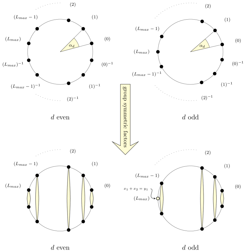
Figure 1: Illustration of the polynomial factorisations for the potential $W_{k}=x_{1}^{d}+x_{2}^{d}$ (upper row) and for the same potential expressed in symmetric coordinates $y_{1}=x_{1}+x_{2}$ and $y_{2}=x_{1}x_{2}$ (lower row) with $\alpha_{d}=\tfrac{2\pi}{d}$ and $L_{max}=\lfloor\tfrac{d-1}{2}\rfloor$. Each node in the upper row corresponds to a polynomial factorisation $(L)\hat{=}\left(x_{1}-e^{i\alpha_{L}}x_{2}\right)$, where $\alpha_{L}=L\alpha_{d}+\alpha_{d}/2$. In the lower diagram, pairs of nodes $(L)$ and $(L)^{-1}$ (corresponding to $\left(x_{1}-e^{-i\alpha_{L}}x_{2}\right)$) are grouped together (indicated by the shape connecting them), and we express the resulting matrix factorisations in $y$-variables as $\left(x_{1}-e^{i\alpha_{L}}x_{2}\right)\left(x_{1}-e^{-i\alpha_{L}}x_{2}\right)=y_{1}^{2}-\beta_{L}y_{2}$.

We can now easily write down matrix factorisations of the superpotential by grouping the product formula above into two polynomial factors $\mathcal{J},\mathcal{E}$. It is very convenient to keep the description in terms of the $x$-variables (indeed there is a faithful functor of the category of matrix factorisations of $W_{k}(y_{i})$ into the category of matrix factorisations of $\tilde{W}_{k}(x_{i})=W_{k}(x_{1}+x_{2},x_{1}x_{2})$ – this will be discussed in appendix B.4). Then, factorisations of $W_{k}(y_{i})$ can be described as

$$\mathcal{J}_{\mathcal{I}}=\prod_{\eta\in\mathcal{I}}(x_{1}-\eta x_{2})\quad,\quad\mathcal{E}_{\mathcal{I}}=\prod_{\eta\in\mathcal{I}^{c}}(x_{1}-\eta x_{2})\ ,$$ (3.42)

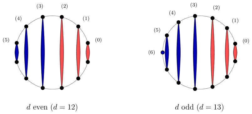
Figure 2: Illustration for the form of the polynomial factorisation $Q_{[0,1,2]}$ corresponding to the CFT boundary condition $|2,0\rangle$. The $\mathcal{J}$ part (containing the roots in $[0,1,2]$) is colored in red (light grey in black-and-white printouts), the $\mathcal{E}$ part (containing the other roots) in blue (dark grey).

where $\mathcal{D}$ is the set of all $d^{\text{th}}$ roots of $-1$, and $\mathcal{I}\subset\mathcal{D}$ is a subset of roots that is invariant under the map $\eta\mapsto\eta^{-1}$. The complement of $\mathcal{I}$ in $\mathcal{D}$ is denoted by $\mathcal{I}^{c}=\mathcal{D}\setminus\mathcal{I}$ (cf. figure 2). These factorisations are quasi-homogeneous in the sense of (3.26). The corresponding matrices $R_{\mathcal{I}}$ are given by

$$R_{\mathcal{I}}=\begin{pmatrix}(1-q_{\mathcal{I}})/2&0\\ 0&(q_{\mathcal{I}}-1)/2\end{pmatrix}\ ,$$ (3.43)

where $q_{\mathcal{I}}=|\mathcal{I}|\frac{2}{d}$ (see (B.5)).

The open string spectrum can be obtained from the open string spectra of permutation factorisations in the product of two minimal models [9] by a suitable projection onto open string states that are symmetric under the exchange of $x_{1}$ and $x_{2}$ (see the discussion in appendix B.4). Essentially, by the projection we get just half the spectrum of the corresponding permutation factorisations, namely the number of bosonic and fermionic fields in the spectrum between two factorisations given by $\mathcal{I}$ and $\mathcal{I}^{\prime}$ is

number of bosons $$=\frac{1}{2}|\mathcal{I}\cap\mathcal{I}^{\prime}|\cdot|\mathcal{I}^{c}\cap\mathcal{I}^{\prime c}|$$ (3.44)

number of fermions $$=\frac{1}{2}|\mathcal{I}^{c}\cap\mathcal{I}^{\prime}|\cdot|\mathcal{I}\cap\mathcal{I}^{\prime c}|\ .$$ (3.45)

The detailed computations are done in appendix B.1. Let us state here only the form of the fermions (see (B.13)),

$$\psi_{p}=p\begin{pmatrix}0&\mathcal{J}_{\mathcal{I}\cap\mathcal{I}^{\prime}}\\ -\mathcal{J}_{\mathcal{I}^{c}\cap\mathcal{I}^{\prime c}}&0\end{pmatrix}\quad\text{with}\ p\in\dfrac{\mathbb{C}[y_{1},y_{2}]}{\left\langle\mathcal{J}_{\mathcal{I}\cap\mathcal{I}^{\prime c}},\mathcal{J}_{\mathcal{I}^{\prime}\cap\mathcal{I}^{c}}\right\rangle}\ .$$ (3.46)

The $U(1)$ charge of a fermion $\psi_{p}$ with a quasi-homogeneous polynomial $p$ is given by

$$q_{\psi_{p}}=\frac{1}{d}\big{(}2\deg(p)+|\mathcal{I}\cap\mathcal{I}^{\prime}|+|\mathcal{I}^{c}\cap\mathcal{I}^{\prime c}|\big{)}\ .$$ (3.47)

The spectrum containing the information on $U(1)$ charges is described by the bosonic and fermionic boundary partition functions (see (B.18) and (B.16))

$$B_{\mathcal{I}\mathcal{I}^{\prime}}(z) =\frac{1-z^{2|\mathcal{I}\cap\mathcal{I}^{\prime}|}}{1-z^{2}}\frac{1-z^{2|\mathcal{I}^{c}\cap\mathcal{I}^{\prime c}|}}{1-z^{4}}z^{|\mathcal{I}^{c}\cap\mathcal{I}^{\prime}|+|\mathcal{I}\cap\mathcal{I}^{\prime c}|}$$ (3.48)

$$F_{\mathcal{I}\mathcal{I}^{\prime}}(z) =\frac{1-z^{2|\mathcal{I}\cap\mathcal{I}^{\prime c}|}}{1-z^{2}}\frac{1-z^{2|\mathcal{I}^{c}\cap\mathcal{I}^{\prime}|}}{1-z^{4}}z^{|\mathcal{I}\cap\mathcal{I}^{\prime}|+|\mathcal{I}^{c}\cap\mathcal{I}^{\prime c}|}\ .$$ (3.49)

These are generating polynomials for the data of the spectrum – the coefficient of a term $z^{n}$ gives the number of morphisms of charge $n/d$.

There are $2^{\lfloor\frac{d+1}{2}\rfloor}-2$ ways of combining the $\lfloor\frac{d+1}{2}\rfloor$ factors into two factors $\mathcal{J}$ and $\mathcal{E}$ (the $-2$ is because we ignore the trivial factorisations where $\mathcal{J}$ or $\mathcal{E}$ are constant). The common feature of these factorisations is that they do not have any fermions in their self-spectrum. As we shall see shortly, these factorisations can only correspond to a subset of the boundary states that we found before. It will therefore be necessary to find other factorisations with higher rank matrices $\mathcal{J},\mathcal{E}$. Some of those will be constructed in section 4.4 by the technique of tachyon condensation.

3.4 RR charges

To determine RR charges we have to compute one-point functions of bulk fields in the presence of a boundary. By spectral flow, the fields corresponding to RR ground states can be labelled by elements of the chiral ring. For such an element $\phi$ we calculate the charge by the Kapustin-Li formula [49] (see also [50]),

$$\text{ch}_{\phi}(Q)=\frac{1}{\sqrt{2}}\text{Res}_{W_{k}}\Big{(}\phi\text{Str}\big{(}\partial_{y_{1}}Q\partial_{y_{2}}Q\big{)}\Big{)}\ .$$ (3.50)

Note that we have to insert a factor $1/\sqrt{2}$ if we want to compare the results to the charges of the full boundary states in the CFT description. (This rescaling of the RR charge also occurs e.g. in [25]). The residue is formally defined as

$$\text{Res}_{W_{k}}(f)=\frac{1}{(2\pi i)^{2}}\oint\oint\frac{f}{\partial_{y_{1}}W_{k}\partial_{y_{2}}W_{k}}dy_{1}dy_{2}\ .$$ (3.51)

It can be evaluated by noting that (see [53])

$$\text{Res}_{W_{k}}(f\partial_{y_{i}}W_{k})=0\quad\text{for all}\ f\ \text{and all}\ y_{i}\ .$$ (3.52)

This fixes the residue up to a normalisation which is given by the requirement that the Hessian determinant $H$,

$$H_{k}=\det(\partial_{y_{i}}\partial_{y_{j}}W_{k})=d^{2}\;y_{2}^{k}\Big{(}(U^{\prime}_{k+1}(z))^{2}-U^{\prime}_{k+2}(z)U^{\prime}_{k}(z)\Big{)}\ ,$$ (3.53)

($z=y_{1}/\sqrt{y_{2}}$) has as residue the number of chiral primary fields,

$$\text{Res}_{W_{k}}(H_{k})=\frac{(k+1)(k+2)}{2}\ .$$ (3.54)

It defines a pairing on the chiral primary fields $\tilde{U}_{(\Lambda_{1},\Lambda_{2})}(y_{1},y_{2})$,

$$\text{Res}_{W_{k}}\big{(}\tilde{U}_{(\Lambda_{1},\Lambda_{2})}\tilde{U}_{(\Lambda_{1}^{\prime},\Lambda_{2}^{\prime})}\big{)}=d^{2}\;\delta_{\Lambda_{1},\Lambda_{1}^{\prime}}\delta_{k-\Lambda_{1}-\Lambda_{2},\Lambda_{2}^{\prime}}\ .$$ (3.55)

Let us now evaluate the RR charge. For a factorisation with a simple factor $\mathcal{J}_{j}=y_{1}^{2}-\beta_{j}y_{2}$ we find

$$\text{Str}\partial_{y_{1}}Q_{j}\partial_{y_{2}}Q_{j}=\frac{d}{z^{2}-\beta_{j}}\Big{(}\beta_{j}U_{k+2}(z)-2zU_{k+1}(z)\Big{)}y_{2}^{k/2}\ .$$ (3.56)

To determine the charge we need to expand this polynomial in combinations of Chebyshev polynomials in $z$, and we claim

$$\frac{1}{z^{2}-\beta_{j}}\left(\beta_{j}U_{k+2}(z)-2zU_{k+1}(z)\right)=2\sum_{i=0}^{\lfloor\frac{k}{2}\rfloor}\cos\big{(}\tfrac{\pi}{d}(2j+1)(i+1)\big{)}U_{k-2i}(z)\ .$$ (3.57)

To prove this we write $z=2\cos t$, and use an alternative expression for the Chebyshev polynomials,

$$U_{n}(2\cos t)=\frac{\sin\big{(}(n+1)t\big{)}}{\sin t}\ .$$ (3.58)

This transforms (3.57) into a trigonometric identity,

$$\beta_{j}\sin\big{(}(k+3)t\big{)}-4\cos t\sin\big{(}(k+2)t\big{)}\\ =2(4\cos^{2}t-\beta_{j})\sum_{i=0}^{\lfloor\frac{k}{2}\rfloor}\Big{(}\cos\big{(}\tfrac{\pi}{d}(2j+1)(i+1)\big{)}\sin\big{(}(k-2i+1)t\big{)}\Big{)}\ ,$$ (3.59)

which can be proved straightforwardly by rewriting the trigonometric functions in terms of exponentials and evaluating the geometric sum on the right hand side.

Using (3.57) and the property (3.55) of the residue, we can evaluate the charge corresponding to the normalised fields $\phi_{i}=d\;U_{k-2i}(z)y_{2}^{k/2}$, and we find

$$\text{ch}_{\phi_{i}}(Q_{j})=\sqrt{2}\cos\tfrac{\pi}{d}(2j+1)(i+1)\ .$$ (3.60)

This describes the charge for any factorisation $Q_{j}$ with a simple factor $\mathcal{J}_{j}=y_{1}^{2}-\beta_{j}y_{2}$. As we will see later in section 4.2, all other polynomial factorisations $Q_{\mathcal{I}}$ can be obtained by taking tachyon condensates of those with a single factor in $\mathcal{J}$. The charges add up in this process, so that the charge of $Q_{\mathcal{I}}$ is given by

$$\text{ch}_{\phi_{i}}(Q_{\mathcal{I}})=\frac{1}{\sqrt{2}}\sum_{\eta\in\mathcal{I}}\eta^{i+1}\ ,$$ (3.61)

where we made use of the formula $\eta_{j}=e^{i\pi\frac{2j+1}{d}}$ for the $d^{\text{th}}$ roots of unity and understand the sum as being taken over those roots $\eta$ appearing in the index set $\mathcal{I}$ of the factorisation $Q_{\mathcal{I}}$ formulated in $x_{i}$ variables.

This ends our discussion of the polynomial factorisations and their properties. Let us now see how these results are related to the CFT analysis.

4 Comparison of factorisations and boundary states

In this section we will finally address the comparison between the boundary states and the matrix factorisations for the $SU(3)/U(2)$-model. We shall first identify the boundary states that correspond to polynomial factorisations – these already form a basis of the vector space of RR charges. We shall then discuss tachyon condensation and RG flows, and show how further boundary states can be identified as matrix factorisations.

4.1 Polynomial factorisations

The simplest factorisations of $W_{k}(y_{1},y_{2})$ are the polynomial factorisations that were identified in section 3.3. One of their properties is that they do not have fermions in their self-spectra. To do the comparison, we first identify the boundary states that lead to fermion-free spectra.

The fermions in the self spectrum of a brane with boundary state $|L,l\rangle$ correspond to chiral primaries in the overlap between $|L,l\rangle$ and $\overline{|L,l\rangle}=|L,k+1-l\rangle$. A chiral primary $((l_{1},l_{2}),0;l_{1},l_{1}+2l_{2})$ appears there with multiplicity $n_{(l_{1},l_{2})L}{}^{L}N^{(k+1)}_{l_{1}l}{}^{k+1-l}$. The second factor describing the fusion rules of $su(2)$ is obviously $0$ when $l=0$ or $l=k+1$ because $l_{1}\leq k$, thus the branes with boundary states $|L,0\rangle$ have fermion-free open string spectra. It turns out that for odd $k$, there are no further boundary states with fermion-free self-spectra; for even $k$ there are in addition the boundary states $|\frac{k}{2},l\rangle$. The detailed analysis can be found in appendix A.3.1.

Let us concentrate on the boundary states $|L,0\rangle$. To characterise them further, we can compute their bosonic spectra. We can show (see appendix A.3.2) that they have $(L+1)(k+1-2L)$ bosons in their self-spectrum. This matches with the number of bosons for polynomial factorisations with $L+1$ elementary factors in $\mathcal{J}$ or $\mathcal{E}$. The boundary state $|0,0\rangle$ therefore seems to correspond to a factorisation with $\mathcal{J}\sim y_{1}^{2}-\beta_{j}y_{2}$ for some $\beta_{j}$. To determine which $\beta_{j}$ is the correct one, we compare the RR charges. The RR charge of the boundary state $|0,0\rangle$ is given by (see (2.40))

$$\text{ch}_{i}(|0,0\rangle)=\frac{1}{\sqrt{2}}\frac{\sin\frac{2\pi}{d}(i+1)}{\sin\frac{\pi}{d}(i+1)}=\sqrt{2}\cos\tfrac{\pi}{d}(i+1)\ ,$$ (4.1)

and by comparison with the RR charges (3.60) of the elementary factorisations, we see that we find agreement for $j=0$. Hence we conclude that $\beta_{0}=2(1+\cos(\frac{\pi}{d}))$ is the correct choice, so that

$$|0,0\rangle\leftrightarrow Q_{|0,0\rangle}=\begin{pmatrix}0&(y_{1}^{2}-\beta_{0}y_{2})\\ \frac{W_{k}}{y_{1}^{2}-\beta_{0}y_{2}}&0\end{pmatrix}\ .$$ (4.2)

The same reasoning applies to the remaining boundary states $|L,0\rangle$ with $L\not=0$ that should correspond to factorisations where $\mathcal{J}$ consists of $L+1$ factors. By evaluating the RR charges we can determine which factors appear, namely we find

$$\text{ch}_{i}(|L,0\rangle) =\frac{1}{\sqrt{2}}\frac{\sin\frac{2\pi}{d}(L+1)(i+1)}{\sin\frac{\pi}{d}(i+1)}$$

$$=\sqrt{2}\sum_{j=0}^{L}\cos\tfrac{\pi}{d}(2j+1)(i+1)$$

$$=\sum_{j=0}^{L}\text{ch}_{i}(Q_{\beta_{j}})\ .$$ (4.3)

We conclude that we have the following correspondence,

$$|L,0\rangle\leftrightarrow Q_{|L,0\rangle}=\begin{pmatrix}0&\prod_{j=0}^{L}(y_{1}^{2}-\beta_{j}y_{2})\\ \frac{W_{k}}{\prod_{j=0}^{L}(y_{1}^{2}-\beta_{j}y_{2})}&0\end{pmatrix}\ .$$ (4.4)

To simplify notation, we define

$$[n_{1},\dotsc,n_{r}]:=\bigcup_{i=1}^{r}\{\eta_{n_{i}},\eta_{n_{i}}^{-1}\}\ ,$$ (4.5)

so that $Q_{|L,0\rangle}=Q_{\mathcal{I}_{|L,0\rangle}}$ with the set of roots given by

$$\mathcal{I}_{|L,0\rangle}=[0,\dotsc,L]\ .$$ (4.6)

It remains to check the relative spectra. Consider the factorisations $Q_{\mathcal{I}_{|L,0\rangle}}$ and $Q_{\mathcal{I}_{|L^{\prime},0\rangle}}$, and assume $L^{\prime}\geq L$. Then $\mathcal{I}_{|L,0\rangle}\subset\mathcal{I}_{|L^{\prime},0\rangle}$, and from (3.45) we see that the spectrum does not contain any fermions. The bosonic spectrum is encoded in the generating polynomial $B_{\mathcal{I}_{|L,0\rangle}\mathcal{I}_{|L^{\prime},0\rangle}}(z)$ given in (3.48). Using

$$|\mathcal{I}_{|L,0\rangle}\cap\mathcal{I}_{|L^{\prime},0\rangle}| =2L+2$$ (4.7)

$$|\mathcal{I}_{|L,0\rangle}^{c}\cap\mathcal{I}_{|L^{\prime},0\rangle}^{c}| =k+3-(2L^{\prime}+2)$$ (4.8)

$$|\mathcal{I}_{|L,0\rangle}^{c}\cap\mathcal{I}_{|L^{\prime},0\rangle}| =2(L^{\prime}-L)$$ (4.9)

$$|\mathcal{I}_{|L,0\rangle}\cap\mathcal{I}_{|L^{\prime},0\rangle}^{c}| =0\ ,$$ (4.10)

the generating polynomial takes the form

$$B_{\mathcal{I}_{|L,0\rangle}\mathcal{I}_{|L^{\prime},0\rangle}}(z) =\sum_{\alpha_{1}=0}^{L}\sum_{\alpha_{2}=0}^{k-2L^{\prime}}z^{4\alpha_{1}+2\alpha_{2}+2(L^{\prime}-L)}$$ (4.11)

$$=\frac{1-z^{2(2L+2)}}{1-z^{4}}\frac{1-z^{2(k+3-(2L^{\prime}+2))}}{1-z^{2}}z^{2(L^{\prime}-L)}\ .$$ (4.12)

This coincides precisely with the generating polynomial $B_{|L,0\rangle,|L^{\prime},0\rangle}(z)$ in (A.26) of the CFT computation. This analysis thus confirms the consistency of the correspondence

$$|L,0\rangle\leftrightarrow Q_{\mathcal{I}_{|L,0\rangle}}\ .$$ (4.13)

Recall that the boundary states $|L,0\rangle$ already form a basis of the charge lattice that is spanned by the maximally symmetric boundary states.

For $k$ odd, these are all boundary states that can be associated to polynomial factorisations of the superpotential. For even $k$, however, we also found the series $|\frac{k}{2},l\rangle$ with fermion-free self-spectra. The analysis of RR charges leads to the identification

$$|\tfrac{k}{2},l\rangle\leftrightarrow Q_{\mathcal{I}_{|\frac{k}{2},l\rangle}}\quad,\quad\mathcal{I}_{|\frac{k}{2},l\rangle}=\{\eta_{-\frac{k}{2}+l+2m}:\ m\in\{0,\dotsc,k-l+1\}\}\ .$$ (4.14)

This identification is also consistent with the spectra, which can be verified by comparing (3.48) and (A.31).

We conclude that all boundary states with fermion-free self-spectra can be matched to polynomial matrix factorisations. There are, however, other boundary states with fermions in their spectra, and also there are polynomial factorisations that do not correspond to any of the maximally symmetric boundary states.

4.2 Tachyon condensation

Our aim is to identify matrix factorisations for the remaining boundary states. We have already seen that the factorisations $Q_{|L,0\rangle}$ form a basis of the space of RR charges. It is therefore conceivable that we can generate all other factorisations from these elementary ones. In this subsection we shall explain the general mechanism of tachyon condensation for matrix factorisations that enables us to construct new factorisations. As an example we shall demonstrate how for even $k$ the factorisations $Q_{|\frac{k}{2},l\rangle}$ can be generated from the generating set $\{Q_{|L,0\rangle}\}$.

Let us first briefly explain how tachyon condensation works in the matrix factorisation description. Suppose we start with the superposition of two boundary conditions corresponding to the direct sum $Q$ of matrix factorisations $Q_{1}$ and $Q_{2}$,

$$Q=\begin{pmatrix}Q_{1}&0\\ 0&Q_{2}\end{pmatrix}\qquad\text{with}\ \sigma=\begin{pmatrix}\sigma_{1}&0\\ 0&\sigma_{2}\end{pmatrix}\ .$$ (4.15)

A fermion $\psi=\psi_{1,2}$ in the spectrum between $Q_{1}$ and $Q_{2}$ corresponds to a fermion $\Psi$ in the self-spectrum of $Q$ of the form

$$\Psi=\begin{pmatrix}0&0\\ \psi&0\end{pmatrix}\ .$$ (4.16)

It is now easy to check that $Q_{\psi}:=Q+\Psi$ is again a matrix factorisation of $W$. We interpret the corresponding boundary condition as the result of the condensation of the fermionic field $\Psi$, and denote this tachyon condensate by

$$(Q_{1}\xrightarrow{\psi}Q_{2})\equiv Q_{\psi}\equiv\begin{pmatrix}Q_{1}&0\\ \psi&Q_{2}\end{pmatrix}\ .$$ (4.17)

In mathematics this procedure is known as cone construction, and the object $Q_{\psi}$ fits into what is called a distinguished triangle (see e.g. [2, 54]),

$$Q_{1}[1]\xrightarrow{\psi[1]}Q_{2}\rightarrow Q_{\psi}\rightarrow Q_{1}\ .$$ (4.18)

It is understood that the first and the last term of the above sequence are identified (therefore the name triangle) up to the action of the shift functor $[1]$ that maps a factorisation $Q$ to its anti-factorisation $Q[1]=\bar{Q}$. In particular, any cyclic shift of objects in (4.18) will yield another valid distinguished triangle. For example, shifting all objects in (4.18) one position to the left will yield a triangle

$$Q_{2}\xrightarrow{\tilde{\psi}[1]}Q_{\psi}\rightarrow Q_{1}\rightarrow Q_{2}[1]\ ,$$ (4.19)

thus we learn that the object $Q_{1}$ can be obtained as a condensate from $Q_{2}[1]$ and $Q_{\psi}$ with some morphism $\tilde{\psi}$. This will be useful in section 4.4.

Let us exemplify this by studying condensates of two polynomial factorisations $Q_{\mathcal{I}}$ and $Q_{\mathcal{I}^{\prime}}$ that at least have one fermion in their relative spectrum. From (3.45) we see that this implies that $\mathcal{I}\not\subset\mathcal{I}^{\prime}$ and $\mathcal{I}^{\prime}\not\subset\mathcal{I}$. Turning on a fermion $\psi_{p}$ (see (3.46)) leads to the factorisation

$$(Q_{\mathcal{I}}\xrightarrow{p}Q_{\mathcal{I}^{\prime}})\equiv(Q_{\mathcal{I}}\xrightarrow{\psi_{p}}Q_{\mathcal{I}^{\prime}})=\begin{pmatrix}0&\mathcal{J}_{\mathcal{I}}&0&0\\ \mathcal{J}_{\mathcal{I}^{c}}&0&0&0\\ 0&p\mathcal{J}_{\mathcal{I}\cap\mathcal{I}^{\prime}}&0&\mathcal{J}_{\mathcal{I}^{\prime}}\\ -p\mathcal{J}_{\mathcal{I}^{c}\cap\mathcal{I}^{\prime c}}&0&\mathcal{J}_{\mathcal{I}^{\prime c}}&0\end{pmatrix}\ .$$ (4.20)

Consider now the fermion of lowest charge ($p=1$). By doing some elementary transformations $Q\to\mathcal{U}Q\mathcal{U}^{-1}$, one can verify that this factorisation is equivalent to a direct sum,

$$(Q_{\mathcal{I}}\xrightarrow{1}Q_{\mathcal{I}^{\prime}})\cong Q_{\mathcal{I}\cap\mathcal{I}^{\prime}}\oplus Q_{\mathcal{I}\cup\mathcal{I}^{\prime}}\ .$$ (4.21)

In case $\mathcal{I}\cap\mathcal{I}^{\prime}=\emptyset$ or $\mathcal{I}\cup\mathcal{I}^{\prime}=\mathcal{D}$, one of the summands is trivial and the condensate is equivalent to a single polynomial factorisation.

For even $k$, we can use the above tachyon condensations to show how we can obtain the polynomial factorisations $Q_{|\frac{k}{2},l\rangle}$ from our generating set $\{Q_{|L,0\rangle}\}$. Of course $Q_{|\frac{k}{2},0\rangle}$ is already contained in the set, so the first non-trivial example is

$$Q_{|\frac{k}{2},1\rangle}=Q_{[0,\dotsc,\frac{k}{2}-1,\frac{k}{2}+1]}\ .$$ (4.22)

From the condensation formula (4.21) we see that

$$Q_{|\frac{k}{2},1\rangle}\cong\left(Q_{|\frac{k}{2}-1,0\rangle}\xrightarrow{1}\overline{Q_{|\frac{k}{2},0\rangle}}\right)\ .$$ (4.23)

To simplify notations, we shall denote the factorisation $Q_{|L,0\rangle}$ by a rectangular box with label $L$, and the factorisation $Q_{\overline{|L,0\rangle}}$ by a rounded box with label $L$, so that the above condensation process reads

$$\raisebox{-4.30554pt}{\includegraphics{figures/KSLGpaper-figA}}\ .$$ (4.24)

It is easy to see how this generalises: for $l\leq\frac{k}{2}$ one has

(4.25)

The case $l\geq\frac{k}{2}+1$ is also covered by noting that $Q_{|\frac{k}{2},l\rangle}=\overline{Q_{|\frac{k}{2},k+1-l\rangle}}$. Note that although multiple arrows appear, the result can still be written as a condensate in the form (4.17) by grouping the factorisations in rectangular boxes into $Q_{1}$ and the ones in rounded boxes into $Q_{2}$.

Before we now go on to construct factorisations for other boundary states, we shall first discuss the analogue of tachyon condensation on the CFT side.

4.3 RG flows

On the CFT side we also have some information on tachyon condensation, which here corresponds to boundary RG flows. There is a general rule for flows in coset models [55, 31] that we can apply in our setup. This rule is based on a conjecture that certain flows that are visible for large coset levels can be extrapolated down to arbitrary levels.

The content of the rule in our case is the following. Choose a representation $\Lambda$ of $su(3)_{k}$, and labels $L,l$ that parameterise boundary states. Then the rule predicts a flow

$$\sum_{\lambda,l^{\prime}}b^{\Lambda}_{\lambda}N^{(k+1)}_{\lambda l}{}^{l^{\prime}}|L,l^{\prime}\rangle\leadsto\sum_{L^{\prime}}n_{\Lambda L}{}^{L^{\prime}}|L^{\prime},l\rangle\ .$$ (4.26)

Here, $b^{\Lambda}_{\lambda}$ denotes the branching coefficient of the regular embedding $su(2)\subset su(3)$ at embedding index $1$, $N^{(k+1)}_{\lambda l}{}^{l^{\prime}}$ is the fusion coefficient of $su(2)$ at level $k+1$ and $n_{\Lambda L}{}^{L^{\prime}}$ the twisted $su(3)$ fusion coefficient at level $k$.

There is a lot of evidence that this rule correctly describes boundary RG flows [31] (see also [56]). As a simple consistency check in our case, we can compare the RR charges of the initial and the final configuration. The charge of the left hand side of equation (4.26) can be evaluated using (2.41),

$$\text{ch}(\text{LHS}) =\sum_{l^{\prime},\lambda,L^{\prime\prime}}b^{\Lambda}_{\lambda}N^{(k+1)}_{\lambda l}{}^{l^{\prime}}(N^{(k+1)}_{LL^{\prime\prime}}{}^{l^{\prime}}-N^{(k+1)}_{LL^{\prime\prime}}{}^{k+1-l^{\prime}})\text{ch}(|L^{\prime\prime},0\rangle)$$

$$=\sum_{l^{\prime},\lambda,L^{\prime\prime}}b^{\Lambda}_{\lambda}N^{(k+1)}_{\lambda L}{}^{l^{\prime}}(N^{(k+1)}_{l^{\prime}L^{\prime\prime}}{}^{l}-N^{(k+1)}_{l^{\prime}L^{\prime\prime}}{}^{k+1-l})\text{ch}(|L^{\prime\prime},0\rangle)$$

$$=\sum_{L^{\prime},\lambda,L^{\prime\prime}}b^{\Lambda}_{\lambda}\big{(}N^{(k+1)}_{\lambda L}{}^{L^{\prime}}-N^{(k+1)}_{\lambda L}{}^{k+1-L^{\prime}}\big{)}\big{(}N^{(k+1)}_{L^{\prime}L^{\prime\prime}}{}^{l}-N^{(k+1)}_{L^{\prime}L^{\prime\prime}}{}^{k+1-l}\big{)}\text{ch}(|L^{\prime\prime},0\rangle)\ .$$ (4.27)

In the last step we split the sum over $l^{\prime}=0,\dotsc,k+1$ into two parts; we introduced the new summation variable $L^{\prime}=0,\dotsc,\lfloor\frac{k}{2}\rfloor$, and replaced $l^{\prime}=L^{\prime}$ in the first part of the sum, and $l^{\prime}=k+1-L^{\prime}$ in the second part. Now let us look at the charge of the right hand side of equation (4.26),

$$\text{ch}(\text{RHS})=\sum_{L^{\prime},L^{\prime\prime}}n_{\Lambda L}{}^{L^{\prime}}\big{(}N^{(k+1)}_{L^{\prime}L^{\prime\prime}}{}^{l}-N^{(k+1)}_{L^{\prime}L^{\prime\prime}}{}^{k+1-l}\big{)}\text{ch}(|L^{\prime\prime},0\rangle)\ .$$ (4.28)

By using formula (2.35) for the twisted $su(3)$ fusion coefficients we find precise agreement with the result (4.27) for the left hand side. This shows that the suggested flows are consistent on the level of RR charges.

Let us work out one class of flows described by the rule above, where we set $\Lambda=(1,0)$. The branching is $(1,0)\to(0)\oplus(1)$, and so from (4.26) we find for $k>1$ the flows

$$|L,l-1\rangle+|L,l\rangle+|L,l+1\rangle\leadsto\left\{\begin{array}[]{ll}|L-1,l\rangle+|L,l\rangle+|L+1,l\rangle&\text{for}\ L\not=\tfrac{k}{2}\\[2.84526pt] |L-1,l\rangle&\text{for}\ L=\tfrac{k}{2}\ .\end{array}\right.$$ (4.29)

Here, labels outside of the allowed range are ignored (e.g. if $l=0$, then the boundary state $|L,l-1\rangle$ on the left hand side does not appear).

The field that triggers these flows is determined as follows: consider the adjoint representation $(1,1)$ of $SU(3)$ and decompose it into the irreducible representations $(l,m)$ of $SU(2)\times U(1)$,

$$(1,1)\longrightarrow(0,0)\oplus(1,3)\oplus(1,-3)\oplus(2,0)\ .$$ (4.30)

The perturbing field then has coset label $((0,0),0;l,m)$ with $l,m$ from the list above. As explained in [55], the adjoint representation $(2,0)$ of $SU(2)\times U(1)$ has to be removed from the list, and choosing the trivial representation $(0,0)$ would correspond to take the identity field for the perturbation. That means that the field $\psi$ responsible for the flows could come from two sectors

$$\psi\in\mathcal{H}_{((0,0),0;1,3)}\oplus\mathcal{H}_{((0,0),0;1,-3)}\ .$$ (4.31)

The field $\psi_{((0,0),0;1,-3)}$ is the superpartner to the chiral primary field $\psi_{((k,0),0;k,k)}$ of charge $q=\frac{k}{k+3}$. This is the charge that we expect to see in the corresponding tachyon condensation processes of matrix factorisations.

4.4 Constructing more factorisations

Having identified the elementary factorisations $Q_{|L,0\rangle}$, we can now use the information on RG flows from the CFT description to obtain new matrix factorisations.

Let us start with a simple example. For $L=\frac{k}{2}$ ($k$ even) and $l=1$, the flow rule (4.29) reads

$$|\tfrac{k}{2},0\rangle+|\tfrac{k}{2},1\rangle+|\tfrac{k}{2},2\rangle\leadsto|\tfrac{k}{2}-1,1\rangle\ .$$ (4.32)

This gives us the prescription how to build the matrix factorisation corresponding to the boundary state $|\frac{k}{2}-1,1\rangle$.The fermion that has to be switched on is also uniquely fixed in this case, because a fermion with charge $\frac{k}{k+3}$ is only found once between $|\frac{k}{2},0\rangle$ and $|\frac{k}{2},1\rangle$, and once between $|\frac{k}{2},2\rangle$ and $|\frac{k}{2},1\rangle$, and both have to be turned on, because otherwise we would end up with a superposition in the condensate. The prescription therefore is

$$Q_{|\frac{k}{2}-1,1\rangle}\cong\big{(}Q_{|\frac{k}{2},0\rangle}\xleftarrow{q_{\psi}=\frac{k}{k+3}}Q_{|\frac{k}{2},1\rangle}\xrightarrow{q_{\psi}=\frac{k}{k+3}}Q_{|\frac{k}{2},2\rangle}\big{)}\ .$$ (4.33)

A comment is in order about the directions of the arrows. We chose the arrows such that we can write the process as a single condensation: we can view it as turning on a single fermion between $Q_{|\frac{k}{2},1\rangle}$ and the superposition of $Q_{|\frac{k}{2},0\rangle}$ and $Q_{|\frac{k}{2},2\rangle}$. It is not difficult to see that reversing both arrows leads to an equivalent factorisation. If we only reverse one arrow, we have to view it as a two-step condensation. If we first condense the right arrow (in whatever direction), we find that there is only one fermion between $Q_{|\frac{k}{2},0\rangle}$ and the condensate, and the corresponding condensate is again equivalent to our first choice of arrows. If we first condense the left arrow (in whatever direction), there are two fermions left. One of them corresponds to the original fermion corresponding to the right arrow, and the condensate is again equivalent to our original choice of arrows. (The other fermion would also lead to a polynomial factorisation, which could not be correct.) Thus, although we do not have a general understanding of how to choose the arrows to reproduce the CFT flows, we see that in our case any choice will lead to the same result.

Let us analyse the condensate in more detail. Identifying the morphisms of the proper charge between the polynomial factorisations on the right hand side of (4.33), we obtain

$$Q_{|\frac{k}{2}-1,1\rangle}\cong\big{(}Q_{[0,\dotsc,\frac{k}{2}]}\xleftarrow{1}Q_{[0,\dotsc,\frac{k}{2}-1,\frac{k}{2}+1]}\xrightarrow{y_{1}}Q_{[0,\dotsc,\frac{k}{2}-2,\frac{k}{2}]}\big{)}\ .$$ (4.34)

The left arrow is a fermion of lowest charge, so we can condense the factorisations according to (4.21) and find

$$Q_{|\frac{k}{2}-1,1\rangle}\cong\big{(}Q_{[0,\dotsc,\frac{k}{2}-1]}\xrightarrow{y_{1}}Q_{[0,\dotsc,\frac{k}{2}-2,\frac{k}{2}]}\big{)}\ .$$ (4.35)

We can rewrite the result in terms of elementary constituents $\{Q_{|L,0\rangle}\}$ by writing the polynomial factorisation on the right of the arrow as a condensate, which leads to

$$\raisebox{-43.05542pt}{\includegraphics{figures/KSLGpaper-figure5}}\ .$$ (4.36)

Thus we have obtained a precise proposal for the matrix factorisation corresponding to $Q_{|\frac{k}{2}-1,1\rangle}$ from the flow rule.

Let us now evaluate the flow rule (4.29) for $l=0$. It then reads for $L<k/2$

$$|L,0\rangle+|L,1\rangle\leadsto|L-1,0\rangle+|L,0\rangle+|L+1,0\rangle\ ,$$ (4.37)

where again boundary states are left out if the label leaves the allowed range. This can be translated into a tachyon condensation in terms of matrix factorisations,

$$\raisebox{-4.30554pt}{\includegraphics{figures/KSLGpaper-figure10}}\ .$$ (4.38)

This tachyon condensate fits into the distinguished triangle (see (4.18))

$$Q_{|L,0\rangle}[1]\xrightarrow{\psi^{*}[1]}Q_{|L,1\rangle}\xrightarrow{}\left(Q_{|L-1,0\rangle}\oplus Q_{|L,0\rangle}\oplus Q_{|L+1,0\rangle}\right)\xrightarrow{}Q_{|L,0\rangle}\ ,$$ (4.39)

where we write $\psi^{*}$ to denote the fermionic morphism of charge $q=\tfrac{k}{k+3}$. By shifting the triangle (see (4.19)) we see that $Q_{|L,1\rangle}$ can be obtained as a condensate from $Q_{|L-1,0\rangle}\oplus Q_{|L,0\rangle}\oplus Q_{|L+1,0\rangle}$ and $Q_{|L,0\rangle}[1]$, i.e. we can invert the tachyon condensation (4.38) to get $Q_{|L,1\rangle}$ alone on the left hand side,

(4.40)

We do not have much control over the morphisms that appear in the condensate, but we see immediately that for $L=\frac{k}{2}-1$ we find the same structure as in (4.36), so the morphisms are fixed for this value of $L$. Assuming that the morphisms will be the same for other values of $L$, we arrive at a proposal for the factorisation corresponding to $Q_{|L,1\rangle}$ ($L<\frac{k}{2}$),

$$\raisebox{-38.74988pt}{\includegraphics{figures/KSLGpaper-figure12}}\ .$$ (4.41)

This representation of $Q_{|L,1\rangle}$ has the advantage that it gives a description directly in terms of the basic constituents $Q_{|L,0\rangle}$. For computations, however, it is more useful to condense the right column of the diagram in (4.41) into the polynomial factorisation $Q_{[0,1,\dotsc,L-1,L+1]}$, so that we find (similarly to (4.35))

$$Q_{|L,1\rangle}\cong\big{(}Q_{[0,1,\dotsc,L]}\xrightarrow{y_{1}}Q_{[0,1,\dotsc,L-1,L+1]}\big{)}\ .$$ (4.42)

In appendix B.2, the fermionic spectrum (including the $U(1)$ charges) of such condensates is investigated, and it agrees with the spectrum of the $|L,1\rangle$ boundary states. Also the relative fermionic spectra among the $Q_{|L,1\rangle}$ and between $Q_{|L,1\rangle}$ and $Q_{|L^{\prime},0\rangle}$ is determined there and shown to be consistent with the CFT results.

Another requirement for our maximally symmetric boundary states is that they are invariant under the exchange of left- and right-movers, because we are considering B-type boundary states in a diagonal theory. On the matrix factorisation side this means to transpose the matrices (see [57, 58]), or, in the above condensation pictures, to reverse the arrows. Let us briefly discuss why reversing the arrow in (4.42) leads to an equivalent factorisation,

$$Q_{\rightarrow}=\big{(}Q_{[0,1,\dotsc,L]}\xrightarrow{y_{1}}Q_{[0,1,\dotsc,L-1,L+1]}\big{)}\cong\big{(}Q_{[0,1,\dotsc,L]}\xleftarrow{y_{1}}Q_{[0,1,\dotsc,L-1,L+1]}\big{)}=Q_{\leftarrow}\ .$$ (4.43)

Displaying only the $\mathcal{J}$-part of the factorisations, we have

$$Q_{\leftarrow}\big{|}_{\mathcal{J}} =\begin{pmatrix}\mathcal{J}_{[0,1,\dotsc,L]}&y_{1}\mathcal{J}_{[0,1,\dotsc,L-1]}\\ 0&\mathcal{J}_{[0,1,\dotsc,L-1,L+1]}\end{pmatrix}$$ (4.44)

$$Q_{\rightarrow}\big{|}_{\mathcal{J}} =\begin{pmatrix}\mathcal{J}_{[0,1,\dotsc,L]}&0\\ y_{1}\mathcal{J}_{[0,1,\dotsc,L-1]}&\mathcal{J}_{[0,1,\dotsc,L-1,L+1]}\end{pmatrix}\ .$$ (4.45)

By just exchanging columns and rows, we can bring $Q_{\leftarrow}\big{|}_{\mathcal{J}}$ to the form

$$Q_{\leftarrow}\big{|}_{\mathcal{J}}\cong\mathcal{J}_{[0,1,\dotsc,L-1]}\begin{pmatrix}\mathcal{J}_{[L+1]}&0\\ y_{1}&\mathcal{J}_{[L]}\end{pmatrix}\ .$$ (4.46)

We can now add the second row to the first with a suitable factor to change the $(1,1)$-entry to $\mathcal{J}_{L}$. Similarly, we use the first column to change the $(2,2)$-entry from $\mathcal{J}_{L}$ to $\mathcal{J}_{L+1}$. Under the combined transformation the $(1,2)$-entry remains zero, and one sees the equivalence to $Q_{\rightarrow}$.

There is a further check that we can perform, namely we can see whether we can reproduce the condensate in (4.38) with a morphism that carries the right charge $q=\frac{k}{k+3}$. Indeed, as discussed in appendix B.3 this is true, so that the RG flow (4.37) is consistent with the identification (4.41) of $|L,1\rangle$.

Having found the factorisations for $|L,1\rangle$, we could now try to go further and construct factorisations for $|L,2\rangle$ by using the RG flow rules. This is possible in principle, but in doing that one encounters the problem that the morphisms that have to be turned on in the condensation are in general not determined uniquely by their $U(1)$ charge. Therefore we have a lot of freedom in the Ansatz for the boundary states with higher label $l$, and it is not clear to us how to determine the right choice. This is related to the fact that for $|L,l\rangle$ with $l\geq 2$ there can be marginal fields in the boundary spectrum, which means that these boundary conditions can be continuously deformed.

Further progress is expected by using topological defect lines that generate the whole spectrum of boundary states. This will be reported elsewhere [59].

5 Low level examples

For the first two levels $k=1$ and $k=2$, the $SU(3)/U(2)$ model corresponds to a minimal model, where all matrix factorisations and boundary states are known. At the next level $k=3$, the $SU(3)/U(2)$ model describes a torus orbifold. In this section we want to compare our results to known results for these low level examples.

5.1 $k=1$

Let us start with $k=1$. The central charge is then $c_{1}=3/2$, which is the central charge of the minimal model $SU(2)/U(1)$ at level $2$. The superpotential is

$$W_{1}(y_{1},y_{2})=y_{1}^{4}-4y_{1}^{2}y_{2}+2y_{2}^{2}\ ,$$ (5.1)

and by replacing $z=\sqrt{2}(y_{2}-y_{1}^{2})$ we obtain

$$\hat{W}_{1}(y_{1},z)=-y_{1}^{4}+z^{2}\ .$$ (5.2)

This is the superpotential of the minimal model of level $2$ with the $0B$ GSO projection. As discussed in [6, 7], the boundary states in this model are labelled by a $su(2)_{2}$ label $\mathcal{L}=0,1,2$, but with the identification rule $|\mathcal{L}\rangle=|2-\mathcal{L}\rangle$. The boundary state $|1\rangle$ that is fixed under this identification is not elementary, but decomposes into two resolved boundary states $|1^{+}\rangle$ and $|1^{-}\rangle$. So there are three boundary states in this model, in concordance with the boundary states $|0,0\rangle$, $\overline{|0,0\rangle}$ and $|0,1\rangle$ that we identified in the $SU(3)/U(2)$ model at level $1$. According to [7] the resolved boundary states $|1^{\pm}\rangle$ correspond to the two polynomial factorisations that exist in this case, which we associated to the boundary states $|0,0\rangle$ and $\overline{|0,0\rangle}$. The remaining boundary state $|0\rangle$ (which corresponds to $|0,1\rangle$ in the $SU(3)/U(2)$ description) then is associated [7] to the factorisation

$$\begin{pmatrix}y_{1}&z\\ -z&-y_{1}^{3}\end{pmatrix}\begin{pmatrix}-y_{1}^{3}&-z\\ z&y_{1}\end{pmatrix}=\hat{W}_{1}(y_{1},z)\cdot\mathbf{1}\ .$$ (5.3)

By a similarity transformation this is equivalent to the factorisation that we found to correspond to $|0,1\rangle$,

$$\begin{pmatrix}y_{1}^{2}-\beta_{0}y_{2}&0\\ y_{1}&y_{1}^{2}-\beta_{1}y_{2}\end{pmatrix}\begin{pmatrix}y_{1}^{2}-\beta_{1}y_{2}&0\\ -y_{1}&y_{1}^{2}-\beta_{0}y_{2}\end{pmatrix}=W_{1}(y_{1},y_{2})\cdot\mathbf{1}\ ,$$ (5.4)

when expressed in $y_{1},z$. Thus our general findings for the $SU(3)/U(2)$ series agree with the minimal model analysis for $k=1$.

5.2 $k=2$

Let us now look at the $SU(3)/U(2)$ model at level $k=2$ with central charge $c_{2}=12/5$. The central charge is that of a minimal model $SU(2)/U(1)$ at level $8$. The superpotential is

$$W_{2} =y_{1}^{5}-5y_{1}^{3}y_{2}+5y_{1}y_{2}^{2}$$

$$=-\frac{1}{4}(y_{1}^{5}-y_{1}z^{2})\ ,$$ (5.5)

where we changed variables by $z=\sqrt{20}(y_{2}-\frac{1}{2}y_{1}^{2})$. This is the superpotential of the D-type minimal model with $0B$ projection. The boundary states are labelled by $|\mathcal{L}\rangle$ and $\overline{|\mathcal{L}\rangle}$, where $\mathcal{L}=0,\dotsc,8$ and we have the identification $|\mathcal{L}\rangle=|8-\mathcal{L}\rangle$, and similarly for the $\overline{|\mathcal{L}\rangle}$. The boundary state $|4\rangle$ is fixed under this identification and can be decomposed into two resolved boundary states $|4^{\pm}\rangle$ (similarly for $\overline{|4\rangle}$). Thus in total we obtain $12$ boundary states. In contrast we only find $8$ boundary states in the $SU(3)/U(2)$ model, and these correspond precisely to the ones with $\mathcal{L}$ even. The reason why we find less is that the $SU(3)/U(2)$ coset algebra is slightly larger than the bosonic subalgebra of the superconformal algebra as it is the chiral algebra of the D-model, which is obtained by a simple-current extension. The boundary states with $\mathcal{L}$ odd correspond to twisted boundary conditions from the point of view of the Kazama-Suzuki model. Indeed, the model at $k=2$ has an additional automorphism. By level-rank duality, we have the equivalence

$$\frac{SU(3)_{2}\times SO(4)_{1}}{U(2)}\cong\frac{SU(4)_{1}\times SO(8)_{1}}{S(U(2)\times U(2))}\ .$$ (5.6)

In the description on the right hand side, it is obvious that we have an additional automorphism that permutes the $U(2)$’s [26]. Using this automorphism to twist the gluing conditions, one finds the missing boundary states. This extra twist is a peculiarity at $k=2$, so we are not going to work out these boundary states explicitly here.

We have listed the (untwisted) boundary states of the Kazama-Suzuki model together with their matrix factorisations in table 1. The corresponding boundary states and factorisations of the minimal models can be found in table 2. It is straightforward to see that the factorisations are related to those in table 1 by similarity transformations, where we can use that

$$y_{1}^{2}-\beta_{0}y_{2} =y_{1}^{2}-\frac{5+\sqrt{5}}{2}y_{2} =-\frac{\sqrt{5}+1}{4}(y_{1}^{2}+z)$$ (5.7)

$$y_{1}^{2}-\beta_{1}y_{2} =y_{1}^{2}-\frac{5-\sqrt{5}}{2}y_{2} =\frac{\sqrt{5}-1}{4}(y_{1}^{2}-z)\ .$$ (5.8)

$|L,l\rangle$	$Q_{|L,l\rangle}$
$|0,0\rangle$	$\begin{pmatrix}0&y_{1}^{2}-\beta_{0}y_{2}\\ y_{1}(y_{1}^{2}-\beta_{1}y_{2})&0\end{pmatrix}$
$|1,0\rangle$	$\begin{pmatrix}0&(y_{1}^{2}-\beta_{0}y_{2})(y_{1}^{2}-\beta_{1}y_{2})\\ y_{1}&0\end{pmatrix}$
$|0,1\rangle$	$\begin{pmatrix}0&0&y_{1}^{2}-\beta_{0}y_{2}&0\\ 0&0&y_{1}&y_{1}^{2}-\beta_{1}y_{2}\\ y_{1}(y_{1}^{2}-\beta_{1}y_{2})&0&0&0\\ -y_{1}^{2}&y_{1}(y_{1}^{2}-\beta_{0}y_{2})\end{pmatrix}$
$|1,1\rangle$	$\begin{pmatrix}0&y_{1}(y_{1}^{2}-\beta_{0}y_{2})\\ (y_{1}^{2}-\beta_{1}y_{2})&0\end{pmatrix}$

Table 1: List of boundary states and their factorisations in the $SU(3)/U(2)$ model at level $k=2$. The other four boundary states are just anti-branes of the ones listed here.

$|\mathcal{L}\rangle$	$Q^{|\mathcal{L}\rangle}$	$|L,l\rangle$
$|0\rangle$	$\begin{pmatrix}0&-\frac{\sqrt{5}+1}{4}(y_{1}^{2}+z)\\ \frac{\sqrt{5}-1}{4}y_{1}(y_{1}^{2}-z)&0\end{pmatrix}$	$|1,0\rangle$
$|2\rangle$	$\begin{pmatrix}0&0&y_{1}&\frac{\sqrt{5}-1}{4}z\\ 0&0&-\frac{\sqrt{5}+1}{4}z&-\frac{1}{4}y_{1}^{3}\\ -\frac{1}{4}y_{1}^{4}&-\frac{\sqrt{5}-1}{4}y_{1}z&0&0\\ \frac{\sqrt{5}+1}{4}y_{1}z&y_{1}^{2}&0&0\end{pmatrix}$	$|0,1\rangle$
$|4^{+}\rangle$	$\begin{pmatrix}0&-\frac{\sqrt{5}+1}{4}(y_{1}^{2}+z)\\ \frac{\sqrt{5}-1}{4}y_{1}(y_{1}^{2}-z)&0\end{pmatrix}$	$|0,0\rangle$
$|4^{-}\rangle$	$\begin{pmatrix}0&-\frac{\sqrt{5}+1}{4}y_{1}(y_{1}^{2}+z)\\ \frac{\sqrt{5}-1}{4}(y_{1}^{2}-z)&0\end{pmatrix}$	$|1,1\rangle$

Table 2: List of boundary states and matrix factorisations in the D-type minimal model $\hat{W}_{2}(y_{1},z)=-\frac{1}{4}(y_{1}^{5}-y_{1}z^{2})$, and the corresponding boundary state in the $SU(3)/U(2)$ Kazama-Suzuki description.

5.3 $k=3$

For $k=3$, the $SU(3)/U(2)$ Kazama-Suzuki model has central charge $c=3$, and the model describes a $\mathbb{Z}_{6}$ orbifold of a torus with complex structure $\tau=\frac{1}{2}(1+i\sqrt{3})$ and size $R=1/\sqrt{3}$ (in units where $\alpha^{\prime}=2$) without a B-field (see [60]). It is a marginal deformation of the product of two minimal models with superpotential $W=v^{6}+w^{3}$. The relation of boundary states and factorisations in that model to the torus orbifold branes has been analysed in [61]. The factorisations we found in the Kazama-Suzuki model can be deformed to factorisations in the product of minimal models. In particular, the deformation of the polynomial factorisations lead to generalised permutation branes in the minimal model description [61].

6 Outlook

In this article we have explored the connection between boundary states and matrix factorisations in the $SU(3)/U(2)$ Kazama-Suzuki model. We have identified matrix factorisations for the series $|L,0\rangle$ of boundary states, which form a basis for the RR charges. By using information on boundary RG flows, we have constructed matrix factorisations also for the series $|L,1\rangle$ as condensates of superpositions of $|L,0\rangle$ branes. This demonstrates the power of tachyon condensation to obtain new factorisations, and it points towards a way of how to obtain all the factorisations corresponding to boundary states $|L,l\rangle$.

The difficulty one faces when extending the analysis to $l\geq 2$ is that these boundary states generically possess marginal boundary fields, and by just looking at the spectrum one will not be able to distinguish those factorisations that are connected by marginal deformations. For this, one needs further information, like the boundary chiral ring.

Another way to single out the factorisations corresponding to the boundary states that are maximally symmetric with respect to the coset W-algebra would be to identify the W-algebra structure on the matrix factorisation side. The Kazama-Suzuki models $SU(n)/U(n-1)$ have an $\mathcal{N}=2$ $W_{n}$ algebra [62, 63, 64, 65]. The construction of the corresponding currents in the bulk LG model for $SU(3)/U(2)$ was done in [67, 68], similarly to the construction of the currents $T$ and $J$ of the $\mathcal{N}=2$ superconformal algebra in [69, 70]. It would be interesting to extend this analysis to boundary theories to understand how the symmetry of the boundary states translates into conditions on matrix factorisations.

A promising way of how to systematically obtain the other factorisations is by employing topological defect lines [71] to generate factorisations for the whole set of boundary states. Topological defects are labelled by representations of the coset algebra. A defect $D_{((0,0),0;1,m)}$ can generate all boundary states $|L,l\rangle$ from the elementary set $\{|L,0\rangle\}$ by fusing the defect onto the boundary. If we identify this defect on the LG side as a factorisation of the difference of two copies of the superpotential [72], we would be in the position to iteratively obtain all relevant matrix factorisations. Of course, one faces also here the problem that one has to fix the freedom of marginally deforming the defect, but once a defect is fixed, there is no further ambiguity for the matrix factorisations corresponding to the maximally symmetric boundary states. This is currently under investigation [59].

The methods of RG flows, tachyon condensations and topological defect lines should also be useful when one approaches the higher rank $SU(n)/U(n-1)$ models for $n\geq 4$. The first task would be to find an elementary set of factorisations corresponding to boundary states $|L,0\rangle$. The connection to a product of $n-1$ minimal models might again be useful, and maybe it is also for this more general setup the permutation factorisations [10] that lead to the relevant factorisations for the Kazama-Suzuki models. Another promising approach would be to use defect lines between the product of minimal models and the Kazama-Suzuki model, similar to the defect corresponding to the functor described in appendix B.4, to relate factorisations on both sides.

Another interesting aspect of the relation of boundary states and factorisations is the charge group. We have different notions of charges in this context, and it would be interesting to compare them. Firstly, we can compute RR charges as one-point functions of the RR fields, which we have used to identify the correct factorisations corresponding to the $|L,0\rangle$ boundary states. This, however, will not be sensible to torsion charges. On the other hand, we can define charges as dynamical invariants. On the CFT side, this means to look for invariants under boundary RG flows like in [73]. For coset models the so defined charge groups [31, 74] are given by equivariant twisted topological K-theory [75, 76]. On the matrix factorisation side, the group of dynamical invariants is the Grothendieck K-group. It would be interesting to understand its connection to the topological K-theory for the Kazama-Suzuki cosets.

Finally, the Kazama-Suzuki models can also be used to construct Gepner-like models [11] for Calabi-Yau compactifications. It would be interesting to repeat the charge analysis of [77] to see whether tensor products of the factorisations that we identified already provide a basis for the charge lattice. Furthermore, it is known that some of the Kazama-Suzuki models can be marginally deformed to obtain other rational models [78], e.g.

$$\frac{SU(3)_{k}}{U(2)}\rightsquigarrow\frac{SU(2)_{k+1}}{U(1)}\times\frac{SU(2)_{\frac{k-1}{2}}}{U(1)}\quad\text{for}\ k\ \text{odd.}$$ (6.1)

In the example above, under the deformation the polynomial factorisations of the Kazama-Suzuki model go over into generalised permutation factorisations [77] of the minimal models. In a full Gepner-like model, it would be interesting to investigate what happens to the properties of the branes (like their mass) when doing complex structure deformations to go one from Gepner-like model to another.

Appendix A CFT open string spectra

A.1 Explicit formula for boundary states

The B-type boundary states $|L,S;l\rangle$ in the $SU(3)_{k}/U(2)$ Kazama-Suzuki model are given by (see equation (2.17))

$$|L,S;l\rangle=\sqrt[4]{\frac{2(k+3)}{3}}\sum_{\Lambda_{1}=0}^{\lfloor\frac{k}{2}\rfloor}\sum_{\lambda=0}^{k+1}\sum_{\Sigma}\frac{\psi_{L(\Lambda_{1},\Lambda_{1})}^{(3)}S^{(so)}_{S\Sigma}S^{(2)}_{l\lambda}}{\sqrt{S^{(3)}_{0(\Lambda_{1},\Lambda_{1})}S^{(so)}_{0\Sigma}S^{(2)}_{0\lambda}}}|(\Lambda_{1},\Lambda_{1}),\Sigma;\lambda,0\rangle\!\rangle\ .$$ (A.1)

Note that in the numerator the untwisted S-matrix $S^{(2)}$ of $SU(2)$ appears because charge conjugation is an inner automorphism for $SU(2)$. The S-matrices for $su(2)_{k+1}$ and $su(3)_{k}$ are given by (see e.g. [44])

$$S^{(2)}_{ll^{\prime}} =\sqrt{\frac{2}{k+3}}\sin\tfrac{\pi(l+1)(l^{\prime}+1)}{k+3}$$ (A.2)

$$S^{(3)}_{0\Lambda} =\frac{8}{\sqrt{3}(k+3)}\sin\tfrac{\pi(\Lambda_{1}+1)}{k+3}\sin\tfrac{\pi(\Lambda_{2}+1)}{k+3}\sin\tfrac{\pi(\Lambda_{1}+\Lambda_{2}+2)}{k+3}\ .$$ (A.3)

For $su(3)$ we only need the S-matrix with one entry $0$.

For $so(4)_{1}$, the modular S-matrix is

$$S^{(so)}=\frac{1}{2}\begin{pmatrix}1&1&1&1\\ 1&1&-1&-1\\ 1&-1&-1&1\\ 1&-1&1&-1\end{pmatrix}\ ,$$ (A.4)

where the rows and columns are indexed by $\Sigma=0,v,s,\bar{s}$.

An expression for the twisted S-matrix $\psi^{(3)}_{L(\Lambda_{1},\Lambda_{1})}$ for $su(3)_{k}$ can be found in [35],

$$\psi^{(3)}_{L(\Lambda_{1},\Lambda_{1})}=\frac{2}{\sqrt{k+3}}\sin\frac{2\pi(L+1)(\Lambda_{1}+1)}{k+3}\ .$$ (A.5)

In the computation of the spectrum we also need the modular S-matrix of $U(1)_{6(k+3)}$,

$$S^{6(k+3)}_{\mu\mu^{\prime}}=\frac{1}{\sqrt{6(k+3)}}\exp\left(-\frac{\pi i}{3(k+3)}\mu\mu^{\prime}\right)\ ,$$ (A.6)

the fusion rules of $su(2)_{k+1}$,

$$N^{(k+1)}_{l_{1}l_{2}}{}^{l_{3}}=\left\{\begin{array}[]{ll}1&\text{for}\ |l_{1}-l_{2}|\leq l_{3}\leq\min(l_{1}+l_{2},2k+2-l_{1}-l_{2})\ \text{and}\ l_{1}+l_{2}+l_{3}\ \text{even}\\ 0&\text{otherwise,}\end{array}\right.$$ (A.7)

and the twisted fusion rules of $su(3)_{k}$, which we discuss next.

A.2 Twisted fusion rules of $su(3)$

The formula for the open string spectra for the B-type branes in the $SU(3)/U(2)$ model contains the twisted fusion rules for $su(3)_{k}$ that are given by

$$n_{\Lambda L}{}^{L^{\prime}}=\sum_{\Lambda^{\prime}=(\Lambda_{1}^{\prime},\Lambda_{1}^{\prime})}\frac{\psi^{(3)}_{L\Lambda^{\prime}}\psi^{(3)}_{L^{\prime}\Lambda^{\prime}}S^{(3)}_{\Lambda\Lambda^{\prime}}}{S^{(3)}_{0\Lambda^{\prime}}}\ .$$ (A.8)

Explicit expressions for these coefficients have been determined in [35] in terms of fusion rules of $su(2)$ at level $2k+4$ (together with an alternative formula involving $su(2)$ fusion at level $(k-1)/2$ for odd $k$). In a similar way one can obtain a formula involving the $su(2)$ fusion rules at level $k+1$ which is the form that is most convenient for our purposes. It is given by (see (2.35))

$$n_{\Lambda L}{}^{L^{\prime}}=\sum_{\gamma}b^{\Lambda}_{\gamma}\big{(}N^{(k+1)}_{\gamma\ L}{}^{L^{\prime}}-N^{(k+1)}_{k+1-\gamma\ L}{}^{L^{\prime}}\big{)}\ ,$$ (A.9)

and it involves the branching coefficients $b$ of the regular embedding of $su(2)$ in $su(3)$ (embedding index $1$).

In the following we shall prove this formula. Let us first note that one can express the twisted S-matrix in terms of the $su(2)$ S-matrix at level $k+1$,

$$\psi^{(3)}_{L(\Lambda_{1},\Lambda_{1})}=\sqrt{2}S^{(2)}_{L,2\Lambda_{1}+1}\ .$$ (A.10)

The ratio $S^{(3)}_{\Lambda\Lambda^{\prime}}/S^{(3)}_{0\Lambda^{\prime}}$ is given by a character $\chi_{\Lambda}$ of the finite dimensional Lie algebra $su(3)$ evaluated on the weight $-\frac{2\pi i}{k+3}(\Lambda^{\prime}+\rho_{su(3)})$, where $\rho_{su(3)}$ is the Weyl vector of $su(3)$ [44, eq.(14.247)]. So we get

$$\frac{S^{(3)}_{\Lambda\Lambda^{\prime}}}{S^{(3)}_{0\Lambda^{\prime}}} =\chi_{\Lambda}(-\tfrac{2\pi i}{k+3}(\Lambda^{\prime}+\rho))$$

$$=\sum_{\gamma}b^{\Lambda}_{\gamma}\chi_{\gamma}(-\tfrac{2\pi i}{k+3}(2\Lambda_{1}^{\prime}+1+\rho_{su(2)}))$$

$$=\sum_{\gamma}b^{\Lambda}_{\gamma}\frac{S^{(2)}_{\gamma,2\Lambda_{1}^{\prime}+1}}{S^{(2)}_{0,2\Lambda_{1}^{\prime}+1}}\ .$$ (A.11)

Here, we expressed the $su(3)$-character $\chi_{\Lambda}$ as a sum of characters $\chi_{\gamma}$ of representations $\gamma$ of $su(2)$ that appear in the decomposition of $\Lambda$. Inserting this into the formula (A.9) for $n$, we obtain

$$n_{\Lambda L}{}^{L^{\prime}} =\sum_{\gamma}b^{\Lambda}_{\gamma}\sum_{\Lambda_{1}^{\prime}=0}^{\lfloor\frac{k}{2}\rfloor}\frac{2S^{(2)}_{L,2\Lambda_{1}^{\prime}+1}S^{(2)}_{L^{\prime},2\Lambda_{1}^{\prime}+1}S^{(2)}_{\gamma,2\Lambda_{1}^{\prime}+1}}{S^{(2)}_{0,2\Lambda_{1}^{\prime}+1}}$$

$$=\sum_{\gamma}\sum_{\mu=0}^{k+1}\frac{S^{(2)}_{L\mu}S^{(2)}_{L^{\prime}\mu}}{S^{(2)}_{0\mu}}\big{(}S^{(2)}_{\gamma\mu}-S^{(2)}_{k+1-\gamma,\mu}\big{)}$$

$$=\sum_{\gamma}b^{\Lambda}_{\gamma}\big{(}N^{(k+1)}_{LL^{\prime}}{}^{\gamma}-N^{(k+1)}_{LL^{\prime}}{}^{k+1-\gamma}\big{)}\ .$$ (A.12)

Here we used that

$$S^{(2)}_{\gamma\mu}-S^{(2)}_{k+1-\gamma,\mu}=\left\{\begin{array}[]{ll}2S^{(2)}_{\gamma\mu}&\text{for $\mu$ odd}\\ 0&\text{for $\mu$ even}\ ,\end{array}\right.$$ (A.13)

and in the last step we used the Verlinde formula for $su(2)_{k+1}$. This concludes the proof of (A.9). Notice that in the formula one could replace the $su(2)_{k+1}$ fusion rules by the untruncated tensor product coefficients of the finite dimensional $su(2)$, because $L+L^{\prime}\leq k$, so no truncation appears.

A.3 Spectra

For the comparison to the matrix factorisation results we are interested in the chiral primaries that appear in the open string spectra. Inserting the result (A.9) into the formula (2.21) for the spectrum, and restricting to chiral primaries, we obtain

$$\langle L_{1},l_{1}|\tilde{q}^{\frac{1}{2}(L_{0}+\bar{L}_{0}-\frac{c}{12})}|L_{2},l_{2}\rangle_{\text{ch.prim.}} =\sum_{\Lambda=(\Lambda_{1},\Lambda_{2})}n_{\Lambda L_{2}}{}^{L_{1}}N^{(k+1)}_{\Lambda_{1}l_{2}}{}^{l_{1}}\chi_{\Lambda,0;\Lambda_{1},\Lambda_{1}+2\Lambda_{2}}(q)$$ (A.14)

$$=\sum_{\Lambda=(\Lambda_{1},\Lambda_{2})}\sum_{\gamma}b^{\Lambda}_{\gamma}\big{(}N^{(k+1)}_{\gamma L_{2}}{}^{L_{1}}-N^{(k+1)}_{k+1-\gamma,L_{2}}{}^{L_{1}}\big{)}$$

$$\qquad\qquad\qquad\times N^{(k+1)}_{\Lambda_{1}l_{2}}{}^{l_{1}}\chi_{\Lambda,0;\Lambda_{1},\Lambda_{1}+2\Lambda_{2}}(q)\ .$$ (A.15)

Here we have used that each chiral primary has a representative $((\Lambda_{1},\Lambda_{2}),0;\Lambda_{1},\Lambda_{1}+2\Lambda_{2})$ (see (2.6)).

To evaluate these expressions we also need a formula for the branching coefficients. The representation $\Lambda=(\Lambda_{1},\Lambda_{2})$ decomposes into $su(2)$-representations according to

$$(\Lambda)\to\bigoplus_{\gamma_{1}=0}^{\Lambda_{1}}\bigoplus_{\gamma_{2}=0}^{\Lambda_{2}}(\gamma_{1}+\gamma_{2})\ .$$ (A.16)

From this we can read off the branching coefficient $b^{\Lambda}_{\gamma}$ that counts how often a representation $\gamma=\gamma_{1}+\gamma_{2}$ appears in the decomposition.

It is sometimes convenient to write the branching coefficients in terms of (untruncated) $su(2)$ fusion rules,

$$b^{(\Lambda_{1},\Lambda_{2})}_{\gamma}=\sum_{\mu}N_{\mu\Lambda_{1}}{}^{\Lambda_{2}}N_{\mu\,\Lambda_{1}+\Lambda_{2}}{}^{2\gamma}\ .$$ (A.17)

A.3.1 Fermions in self spectra

The polynomial matrix factorisations that we found in section 3.3 have the common feature they do not have fermions in their self spectra. In the CFT language this means that there are no chiral primaries in the spectrum between the brane and its anti-brane. We now want to analyse which boundary states satisfy this property. A chiral primary corresponding to the $su(3)_{k}$-representation $\Lambda=(\Lambda_{1},\Lambda_{2})$ appears in the spectrum between $|L,l\rangle$ and $|\overline{L,l}\rangle$ with multiplicity $n_{\Lambda L}{}^{L}N^{(k+1)}_{\Lambda_{1}l}{}^{k+1-l}$. Obviously this is $0$ for $l=0$ or $l=k+1$ because $\Lambda_{1}+\Lambda_{2}\leq k$, so $\Lambda_{1}<k+1$. For $0<l<k+1$, the $su(2)$-fusion coefficient allows all $\Lambda_{1}\geq|k+1-2l|$ that satisfy $\Lambda_{1}+k$ odd. In particular, we can look at the multiplicity of $\Lambda=(k-1,0)$. Evaluating the branching coefficient by formula (A.17) as

$$b^{(k-1,0)}_{\gamma}=N_{k-1,k-1}{}^{2\gamma}\ ,$$ (A.18)

we obtain

$$n_{(k-1,0)L}{}^{L} =\sum_{\gamma=0}^{k-1}\big{(}N_{\gamma L}{}^{L}-N_{k+1-\gamma,L}{}^{L}\big{)}$$

$$=\sum_{\gamma=0}^{k-1}N_{\gamma L}{}^{L}-\sum_{\gamma=2}^{k+1}N_{\gamma L}{}^{L}$$

$$=N_{0L}{}^{L}-N_{kL}{}^{L}\ .$$ (A.19)

In the last step we used that $2L\leq k$. We see that for $L<k/2$, the multiplicity is always one, so only for $L=k/2$ (and thus only for even $k$), there could be further boundary states with fermion-free self-spectra.

Let us now analyse this remaining possibility $L=k/2$ (assuming that $k$ is even). The twisted fusion coefficient $n$ is then

$$n_{(\Lambda_{1},\Lambda_{2})\frac{k}{2}}{}^{\frac{k}{2}} =\sum_{\gamma}b^{\Lambda}_{\gamma}\big{(}N_{\gamma\frac{k}{2}}{}^{\frac{k}{2}}-N_{k+1-\gamma,\frac{k}{2}}{}^{\frac{k}{2}}\big{)}$$

$$=\sum_{\gamma}b^{\Lambda}_{\gamma}(-1)^{\gamma}$$

$$=\sum_{\gamma_{1}=0}^{\Lambda_{1}}\sum_{\gamma_{2}=0}^{\Lambda_{2}}(-1)^{\gamma_{1}+\gamma_{2}}$$

$$=\left\{\begin{array}[]{ll}1&\text{for $\Lambda_{1},\Lambda_{2}$ even}\\ 0&\text{else}\ .\end{array}\right.$$ (A.22)

In the second step we used the expression (A.16) for the branching rules. The twisted fusion rules for $L=k/2$ thus allow for all $\Lambda$ with even labels $\Lambda_{1},\Lambda_{2}$. On the other hand the $su(2)$-fusion coefficient $N^{(k+1)}_{\Lambda_{1}l}{}^{k+1-l}$ vanishes for even $\Lambda_{1}$ if $k$ is even, so there are no chiral primaries in the spectrum between $|\frac{k}{2},l\rangle$ and $|\overline{\frac{k}{2},l}\rangle$.

To summarise, we have identified two series of boundary states that lead to fermion-free self spectra. On the one hand the series $|L,0\rangle$ (and their anti-branes $|L,k+1\rangle$), on the other hand, the series $|\frac{k}{2},l\rangle$, which only exists for even $k$.

A.3.2 Relative spectra of the $l=0$ series

For the series of boundary states $|L,0\rangle$, we shall now determine the spectrum of chiral primaries. We encode the bosonic spectrum (including information on the $U(1)$ charges $q_{i}$) between a boundary state $|L,0\rangle$ and a boundary state $|L^{\prime},0\rangle$ in a generating polynomial,

$$B_{|L,0\rangle,|L^{\prime},0\rangle}(z)=\sum_{\text{chiral primaries}\ \phi_{i}}z^{q_{i}d}\ .$$ (A.23)

Using formula (A.14) for the spectrum, we obtain

$$B_{|L,0\rangle,|L^{\prime},0\rangle}(z) =\sum_{\Lambda}n_{\Lambda L}{}^{L^{\prime}}N^{(k+1)}_{\Lambda_{1}0}{}^{0}z^{\Lambda_{1}+2\Lambda_{2}}$$

$$=\sum_{\Lambda_{2}=0}^{k}n_{(0,\Lambda_{2})L}{}^{L^{\prime}}z^{2\Lambda_{2}}$$

$$=\sum_{\Lambda_{2}=0}^{k}\sum_{\gamma}b_{\gamma}^{(0,\Lambda_{2})}\big{(}N_{\gamma L}{}^{L^{\prime}}-N_{k+1-\gamma,L}{}^{L^{\prime}}\big{)}z^{2\Lambda_{2}}$$

$$=\sum_{\Lambda_{2}=0}^{k}\sum_{\gamma=0}^{\Lambda_{2}}\big{(}N_{\gamma L}{}^{L^{\prime}}-N_{k+1-\gamma,L}{}^{L^{\prime}}\big{)}z^{2\Lambda_{2}}$$

$$=\sum_{\gamma=0}^{k}\sum_{\Lambda_{2}=\gamma}^{k}\big{(}N_{\gamma L}{}^{L^{\prime}}-N_{k+1-\gamma,L}{}^{L^{\prime}}\big{)}z^{2\Lambda_{2}}\ .$$ (A.24)

Now assume that $L^{\prime}\geq L$. Then the representations $\gamma$ that appear in the fusion of $L$ and $L^{\prime}$ can be parameterised as

$$\gamma=L^{\prime}-L+2m\quad\text{with}\ m=0,\dotsc,L\ .$$ (A.25)

So finally we obtain

$$B_{|L,0\rangle,|L^{\prime},0\rangle}(z) =\sum_{m=0}^{L}\Bigg{(}\sum_{\Lambda_{2}=L^{\prime}-L+2m}^{k}z^{2\Lambda_{2}}-\sum_{\Lambda_{2}=k+1-L^{\prime}+2m-L}^{k}z^{2\Lambda_{2}}\Bigg{)}$$

$$=\sum_{m=0}^{L}\sum_{\Lambda_{2}=L^{\prime}-L+2m}^{k-L^{\prime}-L+2m}z^{2\Lambda_{2}}$$

$$=z^{2(L^{\prime}-L)}\frac{1-z^{2(2L+2)}}{1-z^{4}}\frac{1-z^{2(k+3-(2L^{\prime}+2))}}{1-z^{2}}\ .$$ (A.26)

By sending $z\to 1$, we obtain the total number of chiral primaries in the relative spectrum,

$$B_{|L,0\rangle,|L^{\prime},0\rangle}(1)=\frac{1}{2}(2L+2)(k+3-(2L^{\prime}+2))\ .$$ (A.27)

The spectrum encoded in the generating function $B_{|L,0\rangle,|L^{\prime},0\rangle}(z)$ can be compared to the bosonic spectrum between two matrix factorisations. The fermionic spectrum, on the other hand, corresponds to the spectrum of chiral primaries between $|L,0\rangle$ and $|\overline{L^{\prime},0}\rangle$. We have already seen in appendix A.3.1 that there are no such states for $L^{\prime}=L$, and similarly we find

$$F_{|L,0\rangle,|L^{\prime},0\rangle}(1)=\sum_{\Lambda}n_{\Lambda L}{}^{L^{\prime}}N^{(k+1)}_{\Lambda_{1}0}{}^{k+1}=0\ ,$$ (A.28)

because $\Lambda_{1}\leq k$ and so the $su(2)$ fusion rule gives $0$. The $l=0$ series of boundary states should thus correspond to matrix factorisations that do not have any fermions in their relative spectra.

A.3.3 The $L=k/2$ series

For even $k$, we want to analyse the spectra of the boundary states $|\frac{k}{2},l\rangle$. The bosonic partition function $B_{|\frac{k}{2},l\rangle,|\frac{k}{2},l^{\prime}\rangle}(z)$ of chiral primaries is given by

$$B_{|\frac{k}{2},l\rangle,|\frac{k}{2},l^{\prime}\rangle}(z) =\sum_{\Lambda}n_{\Lambda\frac{k}{2}}{}^{\frac{k}{2}}N^{(k+1)}_{\Lambda_{1}l}{}^{l^{\prime}}z^{\Lambda_{1}+2\Lambda_{2}}$$

$$=\sum_{\Lambda_{1}=0,\text{even}}^{k}\sum_{\Lambda_{2}=0,\text{even}}^{k-\Lambda_{1}}N^{(k+1)}_{\Lambda_{1}l}{}^{l^{\prime}}z^{\Lambda_{1}+2\Lambda_{2}}$$

$$=\sum_{\mu=0}^{k/2}N^{(k+1)}_{2\mu,l}{}^{l^{\prime}}\frac{z^{2\mu}-z^{2k+4-2\mu}}{1-z^{4}}\ .$$ (A.29)

In the second step we have used (A.22) to evaluate the twisted fusion rules. From the $su(2)$ fusion coefficient it is immediately clear that the partition function vanishes if $l+l^{\prime}$ is odd. Let us assume thus that $l+l^{\prime}$ is even and that $l^{\prime}\geq l$. For the given range of the labels $\mu,l,l^{\prime}$, we can replace the $su(2)_{k+1}$ fusion rules by the untruncated $su(2)$ tensor product coefficients,

$$N^{(k+1)}_{2\mu l}{}^{l^{\prime}}=N_{2\mu l}{}^{l^{\prime}}-N_{2k+4-2\mu,l}{}^{l^{\prime}}\quad\text{for}\ 2\mu\leq k+2,\ l,l^{\prime}\leq k+1\ .$$ (A.30)

Inserting this into (A.29) we arrive at

$$B_{|\frac{k}{2},l\rangle,|\frac{k}{2},l^{\prime}\rangle}(z) =\sum_{\mu=0}^{k/2}\frac{z^{2\mu}-z^{2k+4-2\mu}}{1-z^{4}}\big{(}N_{2\mu,l}{}^{l^{\prime}}-N_{2k+4-2\mu,l}{}^{l^{\prime}}\big{)}$$

$$=\sum_{\mu=0}^{k/2}\frac{z^{2\mu}-z^{2k+4-2\mu}}{1-z^{4}}N_{2\mu l}{}^{l^{\prime}}-\sum_{\mu=\frac{k}{2}+2}^{k+2}\frac{z^{2k+4-2\mu}-z^{2\mu}}{1-z^{4}}N_{2\mu l}{}^{l^{\prime}}$$

$$=\sum_{\mu\geq 0}\frac{z^{2\mu}-z^{2k+4-2\mu}}{1-z^{4}}N_{2\mu l}{}^{l^{\prime}}$$

$$=\sum_{\mu=(l^{\prime}-l)/2}^{(l+l^{\prime})/2}\frac{z^{2\mu}-z^{2k+4-2\mu}}{1-z^{4}}$$

$$=z^{l^{\prime}-l}\frac{(1-z^{2(l+1)})(1-z^{2(k+2-l^{\prime})})}{(1-z^{2})(1-z^{4})}\ .$$ (A.31)

For the total number of bosons we then have (again assuming $l^{\prime}\geq l$ and $l+l^{\prime}$ even)

$$B_{|\frac{k}{2},l\rangle,|\frac{k}{2},l^{\prime}\rangle}(1)=\frac{1}{2}(l+1)\big{(}k+3-(l^{\prime}+1)\big{)}\ .$$ (A.32)

A.3.4 The $|L,1\rangle$ series

For comparison with the matrix factorisation results we want to determine the fermionic spectra of the $|L,1\rangle$ boundary states, more precisely the self-spectrum as well as the relative spectra among each other and with the $|L,0\rangle$ series.

The fermionic spectrum between $|L_{1},1\rangle$ and $|L_{2},1\rangle$ is the same as the bosonic spectrum between $|L_{1},1\rangle$ and $|L_{2},k\rangle$. The spectrum of chiral primaries is then given by (A.14),

$$\langle L_{1},1|\tilde{q}^{\frac{1}{2}(L_{0}+\bar{L}_{0}-\frac{c}{12})}|L_{2},k\rangle_{\text{ch.prim.}} =\sum_{\Lambda=(\Lambda_{1},\Lambda_{2})}n_{\Lambda L_{2}}{}^{L_{1}}N^{(k+1)}_{\Lambda_{1}1}{}^{k}\chi_{\Lambda,0;\Lambda_{1},\Lambda_{1}+2\Lambda_{2}}(q)$$ (A.33)

$$=\sum_{\Lambda_{2}=0,1}n_{(k-1,\Lambda_{2})L_{2}}{}^{L_{1}}\chi_{(k-1,\Lambda_{2}),0;k-1,k-1+2\Lambda_{2}}(q)\ .$$ (A.34)

Using (A.9) we find

$$n_{(k-1,0)L_{2}}{}^{L_{1}}=n_{(k-1,1)L_{2}}{}^{L_{1}}=N_{0L_{2}}{}^{L_{1}}+N_{1L_{2}}{}^{L_{1}}-N_{kL_{2}}{}^{L_{1}}\ .$$ (A.35)

For the self-spectrum ($L_{1}=L_{2}<\frac{k}{2}$), we therefore find two chiral primaries with $SU(3)$ weights $(k-1,0)$ and $(k-1,1)$, respectively. The $U(1)$ charge of a chiral primary corresponding to $(\Lambda_{1},\Lambda_{2})$ is $q_{(\Lambda_{1},\Lambda_{2})}=\frac{\Lambda_{1}+2\Lambda_{2}}{d}$, in our case the two fermions have $U(1)$ charges

$$q_{(k-1,0)}=\frac{d-4}{d}\quad\text{and}\quad q_{(k-1,1)}=\frac{d-2}{d}\ .$$ (A.36)

For $L_{1}\not=L_{2}$, there are no fermions in the relative spectrum, unless $|L_{1}-L_{2}|=1$. In that case we again find two fermions with the same charges as in (A.36).

The relative fermionic spectrum of $|L_{1},0\rangle$ and $|L_{2},1\rangle$ is the same as the bosonic spectrum between $|L_{1},0\rangle$ and $|L_{2},k\rangle$, which is given by

$$\langle L_{1},0|\tilde{q}^{\frac{1}{2}(L_{0}+\bar{L}_{0}-\frac{c}{12})}|L_{2},k\rangle_{\text{ch.prim.}} =\sum_{\Lambda=(\Lambda_{1},\Lambda_{2})}n_{\Lambda L_{2}}{}^{L_{1}}N^{(k+1)}_{\Lambda_{1}0}{}^{k}\chi_{\Lambda,0;\Lambda_{1},\Lambda_{1}+2\Lambda_{2}}(q)$$ (A.37)

$$=n_{(k,0)L_{2}}{}^{L_{1}}\chi_{(k,0),0;k,k}(q)\ .$$ (A.38)

From (A.9) we conclude that

$$n_{(k,0)L_{2}}{}^{L_{1}}=N_{0L_{2}}{}^{L_{1}}=\delta_{L_{2}L_{1}}\ .$$ (A.39)

Hence, the fermionic spectrum is empty for $L_{1}\not=L_{2}$. For $L_{1}=L_{2}$, there is precisely one fermion in the spectrum of charge

$$q_{(k,0)}=\frac{d-3}{d}\ .$$ (A.40)

Appendix B Landau-Ginzburg open string spectra

In this appendix we shall provide details of the spectrum calculation in the Landau-Ginzburg description of the $SU(3)/U(2)$ Kazama-Suzuki models. We explicitly perform the calculation for the polynomial factorisations, and for the first series of size 2 matrix factorisations corresponding to the boundary states $|L,1\rangle$. We shall then discuss the tachyon condensation that reproduces the RG flow of section 4.3. The final subsection explains the functor from matrix factorisations in the Kazama-Suzuki model to those in the product of minimal models.

B.1 Spectra of polynomial factorisations

The Landau-Ginzburg model corresponding to the $SU(3)/U(2)$ Kazama-Suzuki model at $su(3)$ level $d-3$ has the following superpotential in the variables $y_{1}=x_{1}+x_{2}$ and $y_{2}=x_{1}x_{2}$,

$$W_{k}(y_{1},y_{2})=\prod_{p=0}^{d-1}(x_{1}-\eta_{p}x_{2})=\prod_{j=0}^{\lfloor\frac{d-2}{2}\rfloor}(y_{1}^{2}-\beta_{j}y_{2})\cdot\left\{\begin{array}[]{ll}y_{1}&\text{for $d$ odd}\\ 1&\text{for $d$ even}\end{array}\right.\ ,$$ (B.1)

where

$$\eta_{p}=\exp(i\pi(2p+1)/d)\quad\text{and}\quad\beta_{j}=2+\eta_{j}+\eta_{j}^{-1}\ .$$ (B.2)

The simplest matrix factorisations of $W_{k}$ are of size $1$, i.e. polynomial factorisations. Let $\mathcal{D}=\{\eta|\eta^{d}=-1\}$ be the set of $d^{\text{th}}$ roots of $-1$. Now we can choose a subset $\mathcal{I}\subset\mathcal{D}$ of roots and form the factorisation

$$Q_{\mathcal{I}}=\begin{pmatrix}0&\prod_{\eta\in\mathcal{I}}(x_{1}-\eta x_{2})\\ \prod_{\eta\in\mathcal{I}^{c}}(x_{1}-\eta x_{2})&0\end{pmatrix}\ ,$$ (B.3)

where $\mathcal{I}^{c}=\mathcal{D}\setminus\mathcal{I}$ denotes the complement of $\mathcal{I}$ in $\mathcal{D}$. This describes a factorisation in the $y$-variables provided $\mathcal{I}$ is invariant under $\eta\to\eta^{-1}$.

To determine the infinitesimal $U(1)$ R-charge representation associated to such a matrix factorisation $Q_{\mathcal{I}}$, we make a diagonal Ansatz $R_{\mathcal{I}}=\text{diag}(R_{1},R_{2})$ and plug it into eq. (3.28), finding

$$R_{1}-R_{2}=1-q_{\mathcal{I}}\ ,$$ (B.4)

where $q_{\mathcal{I}}=2|\mathcal{I}|/d$. We want $R_{\mathcal{I}}$ to be traceless [50], so we find

$$R_{\mathcal{I}}=\begin{pmatrix}(1-q_{\mathcal{I}})/2&0\\ 0&(q_{\mathcal{I}}-1)/2\end{pmatrix}\ .$$ (B.5)

We are now ready to explicitly determine the spectra. Let us start with the fermions. For a fermionic morphism $\psi$,

$$\psi=\begin{pmatrix}0&p_{2}\\ p_{1}&0\end{pmatrix}\ ,$$ (B.6)

in the spectrum between $Q_{\mathcal{I}}$ and $Q_{\mathcal{I}^{\prime}}$, the closedness condition reads

$$\begin{pmatrix}0&\mathcal{J}_{\mathcal{I}^{\prime}}\\ \mathcal{J}_{\mathcal{I}^{\prime c}}&0\end{pmatrix}\begin{pmatrix}0&p_{2}\\ p_{1}&0\end{pmatrix}+\begin{pmatrix}0&p_{2}\\ p_{1}&0\end{pmatrix}\begin{pmatrix}0&\mathcal{J}_{\mathcal{I}}\\ \mathcal{J}_{\mathcal{I}^{c}}&0\end{pmatrix}=0\ ,$$ (B.7)

which is equivalent to

$$\mathcal{J}_{\mathcal{I}^{\prime}}p_{1}+p_{2}\mathcal{J}_{\mathcal{I}^{c}}=\mathcal{J}_{\mathcal{I}^{\prime}\cap\mathcal{I}^{c}}(\mathcal{J}_{\mathcal{I}\cap\mathcal{I}^{\prime}}p_{1}+\mathcal{J}_{\mathcal{I}^{c}\cap\mathcal{I}^{\prime c}}p_{2}) =0$$ (B.8)

$$\mathcal{J}_{\mathcal{I}^{\prime c}}p_{2}+p_{1}\mathcal{J}_{\mathcal{I}}=\mathcal{J}_{\mathcal{I}\cap\mathcal{I}^{\prime c}}(\mathcal{J}_{\mathcal{I}\cap\mathcal{I}^{\prime}}p_{1}+\mathcal{J}_{\mathcal{I}^{c}\cap\mathcal{I}^{\prime c}}p_{2}) =0\ .$$ (B.9)

The closed fermionic morphisms thus read

$$\psi_{p}=p(y_{1},y_{2})\begin{pmatrix}0&\mathcal{J}_{\mathcal{I}\cap\mathcal{I}^{\prime}}\\ -\mathcal{J}_{\mathcal{I}^{c}\cap\mathcal{I}^{\prime c}}&0\end{pmatrix}\ ,$$ (B.10)

with some polynomial $p(y_{1},y_{2})$. If $p$ is quasi-homogeneous , the charge of the corresponding fermion $\psi_{p}$ is according to (3.33) given by

$$q_{\psi_{p}}=\frac{1}{d}\big{(}2\text{deg}(p)+\big{|}\mathcal{I}\cap\mathcal{I}^{\prime}\big{|}+\big{|}\mathcal{I}^{c}\cap\mathcal{I}^{\prime c}\big{|}\big{)}\ .$$ (B.11)

The possible choices for $p$ and correspondingly the set of fermions are determined by dividing out exact fermionic morphisms,

$$\widetilde{\psi}=D_{\mathcal{I}\mathcal{I}^{\prime}}\phi =\begin{pmatrix}0&\mathcal{J}_{\mathcal{I}^{\prime}}\\ \mathcal{J}_{\mathcal{I}^{\prime c}}&0\end{pmatrix}\begin{pmatrix}v_{1}&0\\ 0&v_{2}\end{pmatrix}-\begin{pmatrix}v_{1}&0\\ 0&v_{2}\end{pmatrix}\begin{pmatrix}0&\mathcal{J}_{\mathcal{I}}\\ \mathcal{J}_{\mathcal{I}^{c}}&0\end{pmatrix}$$

$$=\begin{pmatrix}0&\mathcal{J}_{\mathcal{I}^{\prime}}v_{2}-v_{1}\mathcal{J}_{\mathcal{I}}\\ \mathcal{J}_{\mathcal{I}^{\prime c}}v_{1}-v_{2}\mathcal{J}_{\mathcal{I}^{c}}&0\end{pmatrix}$$

$$=(\mathcal{J}_{\mathcal{I}^{\prime}\cap\mathcal{I}^{c}}v_{2}-\mathcal{J}_{\mathcal{I}\cap\mathcal{I}^{\prime c}}v_{1})\begin{pmatrix}0&\mathcal{J}_{\mathcal{I}\cap\mathcal{I}^{\prime}}\\ -\mathcal{J}_{\mathcal{I}^{c}\cap\mathcal{I}^{\prime c}}&0\end{pmatrix}\ .$$ (B.12)

Comparing with formula (B.10) for the most general closed fermionic morphism labelled by a polynomial $p$, we see that the elements in the cohomology are of the form

$$\psi_{p}=p\begin{pmatrix}0&\mathcal{J}_{\mathcal{I}\cap\mathcal{I}^{\prime}}\\ -\mathcal{J}_{\mathcal{I}^{c}\cap\mathcal{I}^{\prime c}}&0\end{pmatrix}\quad\text{with}\ p\in\dfrac{\mathbb{C}[y_{1},y_{2}]}{\left\langle\mathcal{J}_{\mathcal{I}\cap\mathcal{I}^{\prime c}},\mathcal{J}_{\mathcal{I}^{\prime}\cap\mathcal{I}^{c}}\right\rangle}\ ,$$ (B.13)

where $\langle\dotsb\rangle$ denotes the ideal generated by the polynomials between the angle brackets. The number of fermionic open string states is given by the dimension of the quotient ring in which $p$ takes it values. According to a generalised Bézout formula [79, Chapter 1, §3.4], the dimension is given by the products of the degrees of the two polynomials defining the ideal, divided by the products of the weights of the variables $y_{i}$. In the case at hand we find

$$n_{\text{fermions}}=\frac{1}{2}\big{|}\mathcal{I}\cap\mathcal{I}^{\prime c}\big{|}\big{|}\mathcal{I}^{\prime}\cap\mathcal{I}^{c}\big{|}\ .$$ (B.14)

Note that at least one of the sets appearing here must have even cardinality: the roots in the sets $\mathcal{I},\mathcal{I}^{\prime}$ appear as pairs $\eta,\eta^{-1}$, and the only single root $\eta=-1$ (that could occur for odd $d$) can only be in either $\mathcal{I}\cap\mathcal{I}^{\prime c}$ or $\mathcal{I}^{\prime}\cap\mathcal{I}^{c}$ because they are disjoint. Let us denote the cardinalities by $n_{1},n_{2}$, where we choose $n_{2}$ to be even. A basis for the quotient ring is then given by monomials $p_{\alpha}=y_{1}^{\alpha_{1}}y_{2}^{\alpha_{2}}$ where $\alpha_{1}=0,\dotsc,n_{1}-1$ and $\alpha_{2}=0,\dotsc,\frac{n_{2}}{2}-1$.

We can go further by not just determining the total number of fermions, but also their $U(1)$ charges given by (B.11). We encode the spectrum in a generating polynomial, the fermionic partition function,

$$F_{\mathcal{I}\mathcal{I}^{\prime}}(z):=\sum_{\text{fermions}\ \Psi^{p}}z^{d\,q_{\Psi^{p}}}\ ,$$ (B.15)

which can straightforwardly be evaluated,

$$F_{\mathcal{I}\mathcal{I}^{\prime}}(z) =\sum_{\alpha_{1}=0}^{n_{1}-1}\sum_{\alpha_{2}=0}^{\frac{n_{2}}{2}-1}z^{2\alpha_{1}+4\alpha_{2}+|\mathcal{I}\cap\mathcal{I}^{\prime}|+|\mathcal{I}^{c}\cap\mathcal{I}^{\prime c}|}$$

$$=\frac{1-z^{2n_{1}}}{1-z^{2}}\frac{1-z^{2n_{2}}}{1-z^{4}}z^{|\mathcal{I}\cap\mathcal{I}^{\prime}|+|\mathcal{I}^{c}\cap\mathcal{I}^{\prime c}|}$$

$$=\frac{1-z^{2|\mathcal{I}\cap\mathcal{I}^{\prime c}|}}{1-z^{2}}\frac{1-z^{2|\mathcal{I}^{c}\cap\mathcal{I}^{\prime}|}}{1-z^{4}}z^{|\mathcal{I}\cap\mathcal{I}^{\prime}|+|\mathcal{I}^{c}\cap\mathcal{I}^{\prime c}|}\ .$$ (B.16)

The analysis for the bosonic morphisms is completely analogous. Note that the bosonic morphisms between $Q_{\mathcal{I}}$ and $Q_{\mathcal{I}^{\prime}}$ are in one-to-one correspondence with the fermions between $Q_{\mathcal{I}}$ and $\overline{Q}_{\mathcal{I}^{\prime}}=Q_{\mathcal{I}^{\prime c}}$; in particular the number of bosons is given by

$$n_{\text{bosons}}=\frac{1}{2}\big{|}\mathcal{I}\cap\mathcal{I}^{\prime}\big{|}\big{|}\mathcal{I}^{c}\cap\mathcal{I}^{\prime c}\big{|}\ ,$$ (B.17)

and the generating polynomial for the bosonic spectrum is

$$B_{\mathcal{I}\mathcal{I}^{\prime}}(z)=\frac{1-z^{2|\mathcal{I}\cap\mathcal{I}^{\prime}|}}{1-z^{2}}\frac{1-z^{2|\mathcal{I}^{c}\cap\mathcal{I}^{\prime c}|}}{1-z^{4}}z^{|\mathcal{I}^{c}\cap\mathcal{I}^{\prime}|+|\mathcal{I}\cap\mathcal{I}^{\prime c}|}\ .$$ (B.18)

Explicitly, the bosons between $Q_{\mathcal{I}}$ and $Q_{\mathcal{I}^{\prime}}$ are given by

$$\phi=v\cdot\begin{pmatrix}\mathcal{J}_{\mathcal{I}^{c}\cap\mathcal{I}^{\prime}}&0\\ 0&\mathcal{J}_{\mathcal{I}\cap\mathcal{I}^{\prime c}}\end{pmatrix}\quad\text{with}\quad v\in\dfrac{\mathbb{C}[y_{1},y_{2}]}{\left\langle\mathcal{J}_{\mathcal{I}\cap\mathcal{I}^{\prime}},\mathcal{J}_{\mathcal{I}^{c}\cap\mathcal{I}^{\prime c}}\right\rangle}\ .$$ (B.19)

B.2 Tachyon condensates of two polynomial factorisations and their spectra

Having identified all polynomial factorisations, a natural procedure to obtain more factorisations is by tachyon condensation. In this section we discuss the situation where we superpose two polynomial factorisations $Q_{\mathcal{I}}$ and $Q_{\mathcal{I}^{\prime}}$ to build the size $2$ factorisation

$$Q_{\mathcal{I}\mathcal{I}^{\prime}}=\begin{pmatrix}Q_{\mathcal{I}}&0\\ 0&Q_{\mathcal{I}^{\prime}}\end{pmatrix}\ ,$$ (B.20)

and then turn on a fermion $\psi_{p^{\tau}}$ between $Q_{\mathcal{I}}$ and $Q_{\mathcal{I}^{\prime}}$ to obtain the tachyon condensate

$$Q_{\mathcal{I}\mathcal{I}^{\prime}}^{\tau}:=(Q_{\mathcal{I}}\xrightarrow{p^{\tau}}Q_{\mathcal{I}^{\prime}})=\begin{pmatrix}Q_{\mathcal{I}}&0\\ \psi_{p^{\tau}}&Q_{\mathcal{I}^{\prime}}\end{pmatrix}\ .$$ (B.21)

The fermion $\psi_{p^{\tau}}$ is of the form (B.13) with some polynomial $p^{\tau}$. For a generic condensate, the $U(1)$ R-charge matrix is given by

$$R=\begin{pmatrix}R_{\mathcal{I}}+\frac{q_{\psi_{p^{\tau}}}-1}{2}\mathbf{1}_{2}&0\\ 0&R_{\mathcal{I}^{\prime}}-\frac{q_{\psi_{p^{\tau}}}-1}{2}\mathbf{1}_{2}\end{pmatrix}\ ,$$ (B.22)

where the charge of the tachyon is given by (B.11). If the condensate matrix $Q^{\tau}_{\mathcal{I}\mathcal{I}^{\prime}}$ is reducible, i.e. if it can be written as a direct sum of smaller factorisations, then the R-charge matrix might have to be modified [50, Section 4.4]. In the case at hand, this only happens for the fermion with lowest charge, $p^{\tau}=1$, in all other cases we can employ (B.22) for the condensate.

B.2.1 Self-spectrum

We first want to determine the self-spectrum of such a factorisation, and we shall restrict the discussion to the fermions. Before the condensation, in the superposition $Q_{\mathcal{I}\mathcal{I}^{\prime}}$ we only have fermions that come from the relative spectra of the constituents, because the polynomial factorisations do not have any fermions in their self-spectra. A basis for the fermionic spectrum is then given by

$$\begin{pmatrix}0&\psi_{\mathcal{I}^{\prime}\mathcal{I}}\\ 0&0\end{pmatrix}\quad\text{and}\quad\begin{pmatrix}0&0\\ \psi_{\mathcal{I}\mathcal{I}^{\prime}}&0\end{pmatrix}\quad\text{with}\ \psi_{\mathcal{I}\mathcal{I}^{\prime}}=p_{\mathcal{I}\mathcal{I}^{\prime}}\begin{pmatrix}0&\mathcal{J}_{\mathcal{I}\cap\mathcal{I}^{\prime}}\\ -\mathcal{J}_{\mathcal{I}^{c}\cap\mathcal{I}^{\prime c}}&0\end{pmatrix}\ ,$$ (B.23)

where $p_{\mathcal{I}\mathcal{I}^{\prime}}\in\frac{\mathbb{C}[y_{1},y_{2}]}{\langle\mathcal{J}_{\mathcal{I}\cap\mathcal{I}^{\prime c}},\mathcal{J}_{\mathcal{I}^{\prime}\cap\mathcal{I}^{c}}\rangle}$ (and according expressions for $\psi_{\mathcal{I}^{\prime}\mathcal{I}}$).

We now want to investigate how the spectrum changes when we turn on the fermion $\psi_{p^{\tau}}$ and form the condensate $Q_{\mathcal{I}\mathcal{I}^{\prime}}^{\tau}$. A fermionic morphism $\Psi$,

$$\Psi=\begin{pmatrix}\psi_{\mathcal{I}\mathcal{I}}&\psi_{\mathcal{I}^{\prime}\mathcal{I}}\\ \psi_{\mathcal{I}\mathcal{I}^{\prime}}&\psi_{\mathcal{I}^{\prime}\mathcal{I}^{\prime}}\end{pmatrix}\ ,$$ (B.24)

in the self-spectrum of $Q^{\tau}_{\mathcal{I}\mathcal{I}^{\prime}}$ is closed with respect to $D^{\tau}$, precisely if the matrix blocks in (B.24) are of the form

$$\psi_{\mathcal{I}\mathcal{I}} =\begin{pmatrix}0&p_{1}\mathcal{J}_{\mathcal{I}\cap\mathcal{I}^{\prime}}\\ p_{2}\mathcal{J}_{\mathcal{I}^{c}\cap\mathcal{I}^{\prime c}}&0\end{pmatrix}$$ (B.25a)

$$\psi_{\mathcal{I}^{\prime}\mathcal{I}} =p\begin{pmatrix}0&\mathcal{J}_{\mathcal{I}\cap\mathcal{I}^{\prime}}\\ -\mathcal{J}_{\mathcal{I}^{c}\cap\mathcal{I}^{\prime c}}&0\end{pmatrix}$$ (B.25b)

$$\psi_{\mathcal{I}\mathcal{I}^{\prime}} =p^{\prime}\begin{pmatrix}0&\mathcal{J}_{\mathcal{I}\cap\mathcal{I}^{\prime}}\\ -\mathcal{J}_{\mathcal{I}^{c}\cap\mathcal{I}^{\prime c}}&0\end{pmatrix}-p_{3}\begin{pmatrix}0&0\\ p^{\tau}\mathcal{J}_{\mathcal{I}^{c}\cap\mathcal{I}^{\prime c}}&0\end{pmatrix}$$ (B.25c)

$$\psi_{\mathcal{I}^{\prime}\mathcal{I}^{\prime}} =\begin{pmatrix}0&p_{2}\mathcal{J}_{\mathcal{I}\cap\mathcal{I}^{\prime}}\\ p_{1}\mathcal{J}_{\mathcal{I}^{c}\cap\mathcal{I}^{\prime c}}&0\end{pmatrix}+p_{3}\begin{pmatrix}0&-\mathcal{J}_{\mathcal{I}^{\prime}}\\ \mathcal{J}_{\mathcal{I}^{\prime c}}&0\end{pmatrix}\ ,$$ (B.25d)

where $p,p^{\prime},p_{1},p_{2},p_{3}$ are polynomials satisfying

$$p\,p^{\tau}=p_{2}\mathcal{J}_{\mathcal{I}\cap\mathcal{I}^{\prime c}}+p_{1}\mathcal{J}_{\mathcal{I}^{c}\cap\mathcal{I}^{\prime}}\ .$$ (B.26)

The space of closed homomorphisms has to be divided by the space of exact homomorphisms. First we observe that

$$D^{\tau}\begin{pmatrix}0&0&0&0\\ 0&0&0&0\\ 0&0&0&0\\ 0&0&0&p_{3}\end{pmatrix}=\begin{pmatrix}0&0&0&0\\ 0&0&0&0\\ 0&0&0&p_{3}\mathcal{J}_{\mathcal{I}^{\prime}}\\ p^{\tau}p_{3}\mathcal{J}_{\mathcal{I}^{c}\cap\mathcal{I}^{\prime c}}&0&-p_{3}\mathcal{J}_{\mathcal{I}^{\prime c}}&0\end{pmatrix}\ ,$$ (B.27)

so by adding this exact homomorphism we can always remove the terms in (B.25) involving $p_{3}$. Next we want to show that given $p$ and $p^{\prime}$, the cohomology class of the homomorphism is already fixed. With fixed $p$ and $p^{\prime}$, the only freedom we have is to change $p_{1},p_{2}$ to some new $p_{1}^{\prime}$ and $p_{2}^{\prime}$. These have to satisfy (B.26), and from that we conclude that

$$p_{1}^{\prime}=p_{1}+p_{4}\mathcal{J}_{\mathcal{I}\cap\mathcal{I}^{\prime c}}\qquad p_{2}^{\prime}=p_{2}-p_{4}\mathcal{J}_{\mathcal{I}^{c}\cap\mathcal{I}^{\prime}}\ ,$$ (B.28)

with some polynomial $p_{4}$. The difference between the corresponding homomorphisms $\Psi^{\prime}$ and $\Psi$ is exact,

$$\Psi^{\prime}-\Psi=\begin{pmatrix}0&p_{4}\mathcal{J}_{\mathcal{I}}&0&0\\ -p_{4}\mathcal{J}_{\mathcal{I}^{c}}&0&0&0\\ 0&0&0&-p_{4}\mathcal{J}_{\mathcal{I}^{\prime}}\\ 0&0&p_{4}\mathcal{J}_{\mathcal{I}^{\prime c}}&0\end{pmatrix}=D^{\tau}\begin{pmatrix}0&0&0&0\\ 0&p_{4}&0&0\\ 0&0&p_{4}&0\\ 0&0&0&0\end{pmatrix}\ .$$ (B.29)

Thus we conclude that the diagonal blocks $\psi_{\mathcal{I}\mathcal{I}}$ and $\psi_{\mathcal{I}^{\prime}\mathcal{I}^{\prime}}$, which are specified by $p_{1}$ and $p_{2}$, do not carry any additional information on the cohomology class that is not contained already in the off-diagonal blocks $\psi_{\mathcal{I}^{\prime}\mathcal{I}}$ and $\psi_{\mathcal{I}\mathcal{I}^{\prime}}$.

Disregarding exact homomorphisms of the form (B.29) or those that would change $p_{3}$, we are now left with exact homomorphisms of the form

$$D^{\tau}\begin{pmatrix}v_{1}\mathbf{1}_{2}&\phi_{\mathcal{I}^{\prime}\mathcal{I}}\\ \phi_{\mathcal{I}\mathcal{I}^{\prime}}&v_{2}\mathbf{1}_{2}\end{pmatrix}=\begin{pmatrix}-\phi_{\mathcal{I}^{\prime}\mathcal{I}}\psi_{p^{\tau}}&D_{\mathcal{I}^{\prime}\mathcal{I}}\phi_{\mathcal{I}^{\prime}\mathcal{I}}\\ D_{\mathcal{I}\mathcal{I}^{\prime}}\phi_{\mathcal{I}\mathcal{I}^{\prime}}+(v_{1}-v_{2})\psi_{p^{\tau}}&\psi_{p^{\tau}}\phi_{\mathcal{I}^{\prime}\mathcal{I}}\end{pmatrix}\ .$$ (B.30)

As we have discussed before, we can concentrate on the off-diagonal blocks $\psi_{\mathcal{I}^{\prime}\mathcal{I}}$ and $\psi_{\mathcal{I}\mathcal{I}^{\prime}}$; they label the fermionic morphisms in the self-spectrum of the tachyon condensate.

From (B.25) we see that (having set $p_{3}=0$) these blocks have the same form as fermions in the superposition of $Q_{\mathcal{I}}$ and $Q_{\mathcal{I}^{\prime}}$ as given by (B.23). The only thing that changes is the condition on the polynomials $p$ and $p^{\prime}$. Let us first look at the upper right block $\psi_{\mathcal{I}^{\prime}\mathcal{I}}$ and the corresponding polynomial $p$. The exact homomorphisms (B.30) together with the condition (B.26) tells us to choose

$$p\in\mathcal{R}=\frac{\mathbb{C}[y_{1},y_{2}]}{\langle\mathcal{J}_{\mathcal{I}\cap\mathcal{I}^{\prime c}},\mathcal{J}_{\mathcal{I}^{c}\cap\mathcal{I}^{\prime}}\rangle}\quad\text{with}\quad p\,p^{\tau}=0\in\mathcal{R}\ .$$ (B.31)

For the lower left block $\psi_{\mathcal{I}\mathcal{I}^{\prime}}$ the changed exactness condition from (B.30) tells us to take

$$p^{\prime}\in\frac{\mathbb{C}[y_{1},y_{2}]}{\langle\mathcal{J}_{\mathcal{I}\cap\mathcal{I}^{\prime c}},\mathcal{J}_{\mathcal{I}^{c}\cap\mathcal{I}^{\prime}},p^{\tau}\rangle}\ .$$ (B.32)

We conclude that some fermions that are present in the superposition survive, while others will disappear due to the changed conditions on $p$ and $p^{\prime}$. The details depend of course crucially on the polynomial $p^{\tau}$ that describes the condensing field. In the extreme case when $p^{\tau}=1$, we see immediately from (B.31) and (B.32) that no fermions would survive.

The condition (B.31) on $p$ and the condition (B.32) on $p^{\prime}$ are dual to each other. We know that there is an exact pairing on $\mathcal{R}$ given by a residue formula (similarly to the one in section 3.4). When we identify $p^{\prime}$’s whose difference is proportional to $p^{\tau}$, the dual space is obtained by restricting $p$ to those polynomials that are orthogonal to $p^{\tau}$ (and everything generated from it) with respect to the pairing. As the residue formula is non-degenerate on $\mathcal{R}$, this is equivalent to saying that $pp^{\tau}=0$ in $\mathcal{R}$.

We can also determine the $U(1)$ charge of these fermions. From the formulae (B.5), (B.22) and (B.11) we conclude that the charge corresponding to a fermion given by the polynomial $p^{\prime}$ is

$$q_{\Psi^{p^{\prime}}}=1+\frac{2}{d}\big{(}\deg p^{\prime}-\deg p^{\tau}\big{)}\ ,$$ (B.33)

the charge of a fermion corresponding to the polynomial $p$ is

$$q_{\Psi^{p}}=\frac{2}{d}\big{(}\deg p+\deg p^{\tau}+|\mathcal{I}\cap\mathcal{I}^{\prime}|+|\mathcal{I}^{c}\cap\mathcal{I}^{\prime c}|\big{)}-1\ .$$ (B.34)

Let us exemplify these considerations in the case of the tachyon condensates (4.42) discussed in section 4.4, namely choosing $Q_{\mathcal{I}},Q_{\mathcal{I}^{\prime}}$ with $\mathcal{I}=[0,\dotsc,L]$ and $\mathcal{I}^{\prime}=[0,\dotsc,L-1,L+1]$, and $p^{\tau}=y_{1}$.

The spectrum is then obtained by evaluating (B.31) and (B.32). The ring in (B.32) in which $p^{\prime}$ takes its values is now

$$p^{\prime}\in\frac{\mathbb{C}[y_{1},y_{2}]}{\langle(y_{1}^{2}-\beta_{L}y_{2}),(y_{1}^{2}-\beta_{L+1}y_{2}),y_{1}\rangle}\ .$$ (B.35)

This ring is one-dimensional, and $p^{\prime}=1$ is a representative for a non-trivial element. Similarly, $p=y_{1}$ is a representative for the solution of $pp^{\tau}=0$ in $\mathcal{R}$ as in (B.31).

The condensate thus has two fermions; according to (B.33) and (B.34) their charges are

$$q_{\Psi^{p^{\prime}}}=\frac{d-2}{2}\quad\text{and}\quad q_{\Psi^{p}}=\frac{d-4}{d}\ .$$ (B.36)

This fits precisely with the CFT result in (A.36).

B.2.2 Relative spectra

Now we want to study the relative fermionic spectrum between two condensates $Q_{i}$ ($i=1,2$) of polynomial factorisations,

$$Q_{i} =(Q_{\mathcal{I}_{i}}\xrightarrow{p^{\tau}_{i}}Q_{\mathcal{I}_{i}^{\prime}})$$ (B.37)

$$=\begin{pmatrix}Q_{\mathcal{I}_{i}}&0\\ \psi_{i}^{\tau}&Q_{\mathcal{I}_{i}^{\prime}}\end{pmatrix}\ ,$$ (B.38)

where

$$\psi^{\tau}_{i}=p_{i}^{\tau}\begin{pmatrix}0&\mathcal{J}_{\mathcal{I}_{i}\cap\mathcal{I}_{i}^{\prime}}\\ -\mathcal{J}_{\mathcal{I}_{i}^{c}\cap\mathcal{I}_{i}^{\prime c}}&0\end{pmatrix}\ .$$ (B.39)

For a fermionic morphism $\Psi_{12}$ from $Q_{1}$ to $Q_{2}$,

$$\Psi_{12}=\begin{pmatrix}\psi_{\mathcal{I}_{1}\mathcal{I}_{2}}&\psi_{\mathcal{I}_{1}^{\prime}\mathcal{I}_{2}}\\ \psi_{\mathcal{I}_{1}\mathcal{I}_{2}^{\prime}}&\psi_{\mathcal{I}_{1}^{\prime}\mathcal{I}_{2}^{\prime}}\end{pmatrix}\ ,$$ (B.40)

the closedness condition reads

$$D_{\mathcal{I}_{1}^{\prime}\mathcal{I}_{2}}\psi_{\mathcal{I}_{1}^{\prime}\mathcal{I}_{2}} =0$$ (B.41)

$$D_{\mathcal{I}_{1}\mathcal{I}_{2}}\psi_{\mathcal{I}_{1}\mathcal{I}_{2}} =-\psi_{\mathcal{I}_{1}^{\prime}\mathcal{I}_{2}}\psi_{1}^{\tau}$$ (B.42)

$$D_{\mathcal{I}_{1}^{\prime}\mathcal{I}_{2}^{\prime}}\psi_{\mathcal{I}_{1}^{\prime}\mathcal{I}_{2}^{\prime}} =-\psi_{2}^{\tau}\psi_{\mathcal{I}_{1}^{\prime}\mathcal{I}_{2}}$$ (B.43)

$$D_{\mathcal{I}_{1}\mathcal{I}_{2}^{\prime}}\psi_{\mathcal{I}_{1}\mathcal{I}_{2}^{\prime}} =-\psi_{2}^{\tau}\psi_{\mathcal{I}_{1}\mathcal{I}_{2}}-\psi_{\mathcal{I}_{1}^{\prime}\mathcal{I}_{2}^{\prime}}\psi_{1}^{\tau}\ .$$ (B.44)

To simplify our analysis, we now specify the precise case that we are interested in. We want in particular to analyse the relative spectra of the factorisations $Q_{|L,1\rangle}$, so we take

$$Q_{1}=Q_{|L_{1},1\rangle} =(Q_{[0,\dotsc,L_{1}-1,L_{1}+1]}\xrightarrow{y_{1}}Q_{[0,\dotsc,L_{1}]})$$ (B.45)

$$Q_{2}=Q_{|L_{2},1\rangle} =(Q_{[0,\dotsc,L_{2}]}\xrightarrow{y_{1}}Q_{[0,\dotsc,L_{2}-1,L_{2}+1]})\ ,$$ (B.46)

and we assume $L_{1}>L_{2}$. Note that we have chosen different presentations for the two factorisations to simplify our analysis (see (4.43)). Explicitly we then have

$$\mathcal{I}_{1} =[0,\dotsc,L_{1}-1,L_{1}+1]\supset[0,\dotsc,L_{2}]=\mathcal{I}_{2}$$ (B.47)

$$\mathcal{I}_{1}^{\prime} =[0,\dotsc,L_{1}]\supset[0,\dotsc,L_{2}-1,L_{2}+1]=\mathcal{I}_{2}^{\prime}\ ,$$ (B.48)

and also $\mathcal{I}_{1}^{\prime}\supset\mathcal{I}_{2}$. This last condition means that there are no fermions in the spectrum between $Q_{\mathcal{I}_{1}^{\prime}}$ and $Q_{\mathcal{I}_{2}}$, i.e. that all closed fermionic morphisms are exact with respect to $D_{\mathcal{I}_{1}^{\prime}\mathcal{I}_{2}}$. On the other hand, the closedness condition (B.41) for the $\psi_{\mathcal{I}_{1}^{\prime}\mathcal{I}_{2}}$-part in the spectrum of the condensates just means that $\psi_{\mathcal{I}_{1}^{\prime}\mathcal{I}_{2}}$ is closed and hence exact with respect to $D_{\mathcal{I}_{1}^{\prime}\mathcal{I}_{2}}$. Also the structure of exact morphisms is unchanged in the $\psi_{\mathcal{I}_{1}^{\prime}\mathcal{I}_{2}}$-sector, so that we can always achieve

$$\psi_{\mathcal{I}_{1}^{\prime}\mathcal{I}_{2}}=0$$ (B.49)

by adding exact morphisms. This simplifies the other closedness conditions (B.42)and (B.43) to the usual closedness conditions of the constituents, and because of the relations in (B.47) and (B.48), all these morphisms are exact and hence can be set to zero,

$$\psi_{\mathcal{I}_{1}\mathcal{I}_{2}} =0$$ (B.50)

$$\psi_{\mathcal{I}_{1}^{\prime}\mathcal{I}_{2}^{\prime}} =0\ .$$ (B.51)

This again simplifies the closedness condition (B.44) to the usual one, and so $\psi_{\mathcal{I}_{1}\mathcal{I}_{2}^{\prime}}$ is of the form

$$\psi_{\mathcal{I}_{1}\mathcal{I}_{2}^{\prime}}=p\begin{pmatrix}0&\mathcal{J}_{\mathcal{I}_{1}\cap\mathcal{I}_{2}^{\prime}}\\ -\mathcal{J}_{\mathcal{I}_{1}^{c}\cap\mathcal{I}_{2}^{\prime c}}&0\end{pmatrix}\ .$$ (B.52)

What happens to the exactness condition? Here we have to distinguish two cases. If $L_{1}>L_{2}+1$, then $\mathcal{I}_{1}\supset\mathcal{I}_{2}^{\prime}$ and thus there are no fermions between $Q_{\mathcal{I}_{1}}$ and $Q_{\mathcal{I}_{2}^{\prime}}$ and we can also set $\psi_{\mathcal{I}_{1}\mathcal{I}_{2}^{\prime}}=0$: in that case there are no fermions in the spectrum.

Let us therefore assume that $L_{1}=L_{2}+1$. We are now looking for the most general exact fermionic morphism $D_{12}\Phi_{12}$ that has all entries vanishing except $\psi_{\mathcal{I}_{1}\mathcal{I}_{2}^{\prime}}$,

$$D_{12}\Phi_{12}=\begin{pmatrix}D_{\mathcal{I}_{1}\mathcal{I}_{2}}\phi_{\mathcal{I}_{1}\mathcal{I}_{2}}-\phi_{\mathcal{I}_{1}^{\prime}\mathcal{I}_{2}}\psi^{\tau}_{1}&D_{\mathcal{I}_{1}^{\prime}\mathcal{I}_{2}}\phi_{\mathcal{I}_{1}^{\prime}\mathcal{I}_{2}}\\ D_{\mathcal{I}_{1}\mathcal{I}_{2}^{\prime}}\phi_{\mathcal{I}_{1}\mathcal{I}_{2}^{\prime}}+\psi^{\tau}_{2}\phi_{\mathcal{I}_{1}\mathcal{I}_{2}}-\phi_{\mathcal{I}_{1}^{\prime}\mathcal{I}_{2}^{\prime}}\psi^{\tau}_{1}&D_{\mathcal{I}_{1}^{\prime}\mathcal{I}_{2}^{\prime}}\phi_{\mathcal{I}_{1}^{\prime}\mathcal{I}_{2}^{\prime}}-\psi^{\tau}_{2}\phi_{\mathcal{I}_{1}^{\prime}\mathcal{I}_{2}}\end{pmatrix}=\begin{pmatrix}0&0\\ \psi^{\text{ex}}_{\mathcal{I}_{1}\mathcal{I}_{2}^{\prime}}&0\end{pmatrix}\ .$$ (B.53)

First we note that $\phi_{\mathcal{I}_{1}^{\prime}\mathcal{I}_{2}}$ has to be closed with respect to $D_{\mathcal{I}_{1}^{\prime}\mathcal{I}_{2}}$, and so it is of the form

$$\phi_{\mathcal{I}_{1}^{\prime}\mathcal{I}_{2}}=v_{1}\begin{pmatrix}\mathcal{J}_{\mathcal{I}_{1}^{\prime c}\cap\mathcal{I}_{2}}&0\\ 0&\mathcal{J}_{\mathcal{I}_{1}^{\prime}\cap\mathcal{I}_{2}^{c}}\end{pmatrix}\ ,$$ (B.54)

with some arbitrary polynomial $v_{1}$. A straightforward analysis yields the form of $\phi_{\mathcal{I}_{1}\mathcal{I}_{2}}$,

$$\phi_{\mathcal{I}_{1}\mathcal{I}_{2}}=\begin{pmatrix}v_{2}\mathcal{J}_{\mathcal{I}_{1}^{c}\cap\mathcal{I}_{1}^{\prime c}\cap\mathcal{I}_{2}}&0\\ 0&v_{2}^{\prime}\mathcal{J}_{\mathcal{I}_{1}\cap\mathcal{I}_{1}^{\prime}\cap\mathcal{I}_{2}^{c}}\end{pmatrix}\ ,$$ (B.55)

with

$$v_{2}^{\prime}\mathcal{J}_{\mathcal{I}_{1}^{c}\cap\mathcal{I}_{1}^{\prime}\cap\mathcal{I}_{2}}-v_{2}\mathcal{J}_{\mathcal{I}_{1}\cap\mathcal{I}_{1}^{\prime c}\cap\mathcal{I}_{2}^{c}}=v_{1}p_{1}^{\tau}\ .$$ (B.56)

In our case the polynomial accompanying $v_{2}^{\prime}$ is $\mathcal{J}_{\mathcal{I}_{1}^{c}\cap\mathcal{I}_{1}^{\prime}\cap\mathcal{I}_{2}}=1$ because $\mathcal{I}_{1}\supset\mathcal{I}_{2}$, so that we can express $v_{2}^{\prime}$ in terms of the other polynomials, and we get

$$\phi_{\mathcal{I}_{1}\mathcal{I}_{2}}=v_{2}\begin{pmatrix}1&0\\ 0&\mathcal{J}_{\mathcal{I}_{1}\cap\mathcal{I}_{2}^{c}}\end{pmatrix}+\begin{pmatrix}0&0\\ 0&v_{1}p_{1}^{\tau}\mathcal{J}_{\mathcal{I}_{1}\cap\mathcal{I}_{1}^{\prime}\cap\mathcal{I}_{2}^{c}}\end{pmatrix}\ .$$ (B.57)

Similarly we have

$$\phi_{\mathcal{I}_{1}^{\prime}\mathcal{I}_{2}^{\prime}}=v_{3}\begin{pmatrix}1&0\\ 0&\mathcal{J}_{\mathcal{I}_{1}^{\prime}\cap\mathcal{I}_{2}^{\prime c}}\end{pmatrix}-\begin{pmatrix}0&0\\ 0&v_{1}p_{2}^{\tau}\mathcal{J}_{\mathcal{I}_{1}^{\prime}\cap\mathcal{I}_{2}^{c}\cap\mathcal{I}_{2}^{\prime c}}\end{pmatrix}\ .$$ (B.58)

Parameterising

$$\phi_{\mathcal{I}_{1}\mathcal{I}_{2}^{\prime}}=\begin{pmatrix}v_{4}&0\\ 0&v_{5}\end{pmatrix}\ ,$$ (B.59)

the $\psi^{\text{ex}}_{\mathcal{I}_{1}\mathcal{I}_{2}^{\prime}}$ component of an exact morphism of the form (B.53) reads

$$\psi^{\text{ex}}_{\mathcal{I}_{1}\mathcal{I}_{2}^{\prime}}=\big{(}v_{5}\mathcal{J}_{[L_{1}]}-v_{4}\mathcal{J}_{[L_{1}-1,L_{1}+1]}-p^{\tau}_{1}v_{3}\mathcal{J}_{[L_{1}-1]}+p_{2}^{\tau}v_{2}\mathcal{J}_{[L_{1}+1]}+v_{1}p^{\tau}_{1}p^{\tau}_{2}\big{)}\begin{pmatrix}0&\mathcal{J}_{\mathcal{I}_{1}\cap\mathcal{I}_{2}^{\prime}}\\ -\mathcal{J}_{\mathcal{I}_{1}^{c}\cap\mathcal{I}_{2}^{\prime c}}&0\end{pmatrix}\ .$$ (B.60)

Comparing this with the form (B.52) of a closed morphism, we see that the fermions in the spectrum are labelled by the quotient ring

$$\mathcal{R}_{12}=\frac{\mathbb{C}[y_{1},y_{2}]}{\langle\mathcal{J}_{[L_{1}]},\mathcal{J}_{[L_{1}-1,L_{1}+1]},p^{\tau}_{1}\mathcal{J}_{[L_{1}-1]},p^{\tau}_{2}\mathcal{J}_{[L_{1}+1]},p^{\tau}_{1}p^{\tau}_{2}\rangle}\ .$$ (B.61)

In our case $p^{\tau}_{1}=p^{\tau}_{2}=y_{1}$, and so

$$\mathcal{R}_{12}=\frac{\mathbb{C}[y_{1},y_{2}]}{\langle y_{1}^{2},y_{2}\rangle}\ ,$$ (B.62)

which is two-dimensional with representatives $p=1,y_{1}$. We finally conclude that there are two fermions in the spectrum between $Q_{|L_{1},1\rangle}$ and $Q_{|L_{1}-1,1\rangle}$.

The charges of these two fermions can then be determined using the charge matrix (B.22) and we obtain

$$q=\frac{d-4}{d}+\frac{2}{d}\text{deg}(p)\ ,$$ (B.63)

so the two fermions have charges $\frac{d-4}{d}$ and $\frac{d-2}{d}$. This matches the CFT result in appendix A.3.4 (see the discussion below (A.36)).

B.2.3 Relative spectrum with polynomial factorisations

We want to determine the fermionic spectrum between a polynomial factorisation $Q_{1}=Q_{\mathcal{I}_{1}}$ and the condensate $Q_{2}$ of two polynomial factorisations,

$$Q_{2}=(Q_{\mathcal{I}_{2}}\xrightarrow{p^{\tau}}Q_{\mathcal{I}_{2}^{\prime}})\ .$$ (B.64)

A closed fermion,

$$\Psi=\begin{pmatrix}\psi_{\mathcal{I}_{1}\mathcal{I}_{2}}\\ \psi_{\mathcal{I}_{1}\mathcal{I}_{2}^{\prime}}\end{pmatrix}\ ,$$ (B.65)

satisfies

$$\psi_{\mathcal{I}_{1}\mathcal{I}_{2}} =p_{1}\begin{pmatrix}0&\mathcal{J}_{\mathcal{I}_{1}\cap\mathcal{I}_{2}}\\ -\mathcal{J}_{\mathcal{I}_{1}^{c}\cap\mathcal{I}_{2}^{c}}&0\end{pmatrix}$$ (B.66)

$$\psi_{\mathcal{I}_{1}\mathcal{I}_{2}^{\prime}} =\begin{pmatrix}0&p_{2}\mathcal{J}_{\mathcal{I}_{1}\cap\mathcal{I}_{2}\cap\mathcal{I}_{2}^{\prime}}\\ p_{2}^{\prime}\mathcal{J}_{\mathcal{I}_{1}^{c}\cap\mathcal{I}_{2}^{c}\cap\mathcal{I}_{2}^{\prime c}}&0\end{pmatrix}\ ,$$ (B.67)

with

$$p_{2}^{\prime}\mathcal{J}_{\mathcal{I}_{1}\cap\mathcal{I}_{2}^{c}\cap\mathcal{I}_{2}^{\prime}}+p_{2}\mathcal{J}_{\mathcal{I}_{1}^{c}\cap\mathcal{I}_{2}\cap\mathcal{I}_{2}^{\prime c}}=p_{1}p^{\tau}\ .$$ (B.68)

In the cases we are interested in, we have either $\mathcal{I}_{1}\subset\mathcal{I}_{2}$ or $\mathcal{I}_{2}\subset\mathcal{I}_{1}$, i.e. there are no fermions between $Q_{\mathcal{I}_{1}}$ and $Q_{\mathcal{I}_{2}}$. By condensation, the closedness and exactness condition do not change for the $\psi_{\mathcal{I}_{1}\mathcal{I}_{2}}$ component, and we can use exact morphisms to set $p_{1}$ to $0$. Then $\psi_{\mathcal{I}_{1}\mathcal{I}_{2}^{\prime}}$ is closed with respect to $D_{\mathcal{I}_{1}\mathcal{I}_{2}^{\prime}}$,

$$\psi_{\mathcal{I}_{1}\mathcal{I}_{2}^{\prime}}=p\begin{pmatrix}0&\mathcal{J}_{\mathcal{I}_{1}\cap\mathcal{I}_{2}^{\prime}}\\ -\mathcal{J}_{\mathcal{I}_{1}^{c}\cap\mathcal{I}_{2}^{\prime c}}&0\end{pmatrix}\ .$$ (B.69)

The remaining exact morphisms $D_{12}\Phi$ then come from bosons

$$\Phi=\begin{pmatrix}{c}\phi_{\mathcal{I}_{1}\mathcal{I}_{2}}\\ \phi_{\mathcal{I}_{1}\mathcal{I}_{2}^{\prime}}\end{pmatrix}\ ,$$ (B.70)

where $\phi_{\mathcal{I}_{1}\mathcal{I}_{2}}$ is closed with respect to $D_{\mathcal{I}_{1}\mathcal{I}_{2}}$,

$$\phi_{\mathcal{I}_{1}\mathcal{I}_{2}}=v_{1}\begin{pmatrix}\mathcal{J}_{\mathcal{I}_{1}^{c}\cap\mathcal{I}_{2}}&0\\ 0&\mathcal{J}_{\mathcal{I}_{1}\cap\mathcal{I}_{2}^{c}}\end{pmatrix}\ ,$$ (B.71)

with some polynomial $v_{1}$. Writing the bosonic component $\phi_{\mathcal{I}_{1}\mathcal{I}_{2}^{\prime}}$ as

$$\phi_{\mathcal{I}_{1}\mathcal{I}_{2}^{\prime}}=\begin{pmatrix}v_{2}&0\\ 0&v_{2}^{\prime}\end{pmatrix}\ ,$$ (B.72)

the remaining exact fermionic morphisms $\Psi^{\text{ex}}$ have $\psi^{\text{ex}}_{\mathcal{I}_{1}\mathcal{I}_{2}}=0$ and

$$\psi^{\text{ex}}_{\mathcal{I}_{1}\mathcal{I}_{2}^{\prime}} =\begin{pmatrix}0&v_{2}^{\prime}\mathcal{J}_{\mathcal{I}_{2}^{\prime}}-v_{2}\mathcal{J}_{\mathcal{I}_{1}}+p^{\tau}v_{1}\mathcal{J}_{\mathcal{I}_{1}\cap\mathcal{I}_{2}^{c}}\mathcal{J}_{\mathcal{I}_{2}\cap\mathcal{I}_{2}^{\prime}}\\ v_{2}\mathcal{J}_{\mathcal{I}_{2}^{\prime c}}-v_{2}^{\prime}\mathcal{J}_{\mathcal{I}_{1}^{c}}-p^{\tau}v_{1}\mathcal{J}_{\mathcal{I}_{1}^{c}\cap\mathcal{I}_{2}}\mathcal{J}_{\mathcal{I}_{2}^{c}\cap\mathcal{I}_{2}^{\prime c}}&0\end{pmatrix}$$ (B.73)

$$=(v_{2}^{\prime}\mathcal{J}_{\mathcal{I}_{1}^{c}\cap\mathcal{I}_{2}^{\prime}}-v_{2}\mathcal{J}_{\mathcal{I}_{1}\cap\mathcal{I}_{2}^{\prime c}}+p^{\tau}v_{1}\mathcal{J}_{\mathcal{I}_{1}\cap\mathcal{I}_{2}^{c}\cap\mathcal{I}_{2}^{\prime c}}\mathcal{J}_{\mathcal{I}_{1}^{c}\cap\mathcal{I}_{2}\cap\mathcal{I}_{2}^{\prime}})\begin{pmatrix}0&\mathcal{J}_{\mathcal{I}_{1}\cap\mathcal{I}_{2}^{\prime}}\\ -\mathcal{J}_{\mathcal{I}_{1}^{c}\cap\mathcal{I}_{2}^{\prime c}}&0\end{pmatrix}\ .$$ (B.74)

Here we used again that either $\mathcal{I}_{1}\subset\mathcal{I}_{2}$ or vice versa. The fermions are then labelled by polynomials $p$ (see (B.69)) modulo identifications that come from the exact morphisms (B.74), hence we can view $p$ as living in the quotient

$$p\in\frac{\mathbb{C}[y_{1},y_{2}]}{\langle\mathcal{J}_{\mathcal{I}_{1}^{c}\cap\mathcal{I}_{2}^{\prime}},\mathcal{J}_{\mathcal{I}_{1}\cap\mathcal{I}_{2}^{\prime c}},p^{\tau}\mathcal{J}_{\mathcal{I}_{1}\cap\mathcal{I}_{2}^{c}\cap\mathcal{I}_{2}^{\prime c}}\mathcal{J}_{\mathcal{I}_{1}^{c}\cap\mathcal{I}_{2}\cap\mathcal{I}_{2}^{\prime}}\rangle}\ .$$ (B.75)

For explicitness we now set

$$\mathcal{I}_{1} =[0,\dotsc,L_{1}]$$ (B.76)

$$\mathcal{I}_{2} =[0,\dotsc,L_{2}]$$ (B.77)

$$\mathcal{I}_{2}^{\prime} =[0,\dotsc,L_{2}-1,L_{2}+1]$$ (B.78)

$$p^{\tau} =y_{1}\ .$$ (B.79)

For $L_{1}<L_{2}$ we have $\mathcal{J}_{\mathcal{I}_{1}\cap\mathcal{I}_{2}^{\prime c}}=1$, so there are no fermions. Similarly for $L_{1}>L_{2}$ we have $\mathcal{J}_{\mathcal{I}_{1}^{c}\cap\mathcal{I}_{2}^{\prime}}=1$, and no fermion remains. On the other hand, for $L_{1}=L_{2}$, the spectrum is given by

$$p\in\frac{\mathbb{C}[y_{1},y_{2}]}{\langle\mathcal{J}_{[L_{1}+1]},\mathcal{J}_{[L_{1}]},y_{1}\rangle}\ ,$$ (B.80)

which is one-dimensional. In conclusion, we find precisely one fermion in the spectrum between $Q_{|L_{1},0\rangle}$ and $Q_{|L_{2},1\rangle}$ if $L_{1}=L_{2}$, and no fermions otherwise. The fermion that appears for $L_{1}=L_{2}$ has charge

$$q=\frac{d-3}{d}\ ,$$ (B.81)

which can be determined using (3.33) and the charge matrices (B.5) and (B.22). This coincides with the CFT result in (A.40).

B.3 Reproducing the CFT flows

Having identified matrix factorisations for the $|L,0\rangle$ and $|L,1\rangle$ series, we can now compare the RG flows (4.29) between boundary states to tachyon condensation in the matrix factorisation language. Let us consider the RG flow

$$|L,0\rangle+|L,1\rangle\leadsto|L-1,0\rangle+|L,0\rangle+|L+1,0\rangle\ .$$ (B.82)

From formula (A.40) we can see that in the relative spectrum between $|L,0\rangle$ and $|L,1\rangle$, there is precisely one fermion $\psi$ of charge $q_{\psi}=\frac{d-3}{d}$. Condensing this fermion corresponds in the CFT to perturb with a field from this coset sector, so this is compatible with the considerations that led to (4.31). In the language of matrix factorisations this fermion is given by (B.69) with $p=1$.

Let us explicitly work out the tachyon condensate. To make the equations more readable, we only write the $\mathcal{J}$-part of the matrix in a notation like in (3.24). We obtain

$$(Q_{|L,0\rangle}\xrightarrow{\psi}Q_{|L,1\rangle})_{\mathcal{J}}=\begin{pmatrix}\mathcal{J}_{[0,\dotsc,L]}&0&0\\ 0&\mathcal{J}_{[0,\dotsc,L]}&0\\ \mathcal{J}_{[0,\dotsc,L-1]}&y_{1}\mathcal{J}_{[0,\dotsc,L-1]}&\mathcal{J}_{[0,\dotsc,L-1,L+1]}\end{pmatrix}\ .$$ (B.83)

We can use the term $\mathcal{J}_{[0,\dotsc,L-1]}$ to eliminate all other entries in that row or column by elementary transformations. Having done this one can immediately see the equivalence to the matrix

$$\big{(}Q_{|L-1,0\rangle+|L,0\rangle+|L+1,0\rangle}\big{)}_{\mathcal{J}}=\begin{pmatrix}\mathcal{J}_{[0,\dotsc,L-1]}&0&0\\ 0&\mathcal{J}_{[0,\dotsc,L]}&0\\ 0&0&\mathcal{J}_{[0,\dotsc,L+1]}\end{pmatrix}\ .$$ (B.84)

This reproduces the RG flow (B.82) in terms of matrix factorisations. Note that the brane $|L,0\rangle$, although appearing in both the initial and the final configuration, is not purely a spectator brane, but is involved in the flow.

B.4 A faithful functor

Given a matrix factorisation $Q(y_{1},y_{2})$ for the superpotential $W_{k}(y_{1},y_{2})$, we can construct from it a matrix factorisation $\tilde{Q}(x_{1},x_{2}):=Q(x_{1}+x_{2},x_{1}x_{2})$ of the superpotential

$$\tilde{W}_{k}(x_{1},x_{2})=W_{k}(x_{1}+x_{2},x_{1}x_{2})=x_{1}^{k+3}+x_{2}^{k+3}\ .$$ (B.85)

This map gives rise to a functor from the category of matrix factorisations of $W_{k}$ to the category of $\tilde{W}_{k}$. It maps a morphism $\Phi(y_{1},y_{2})$ from $Q_{1}$ to $Q_{2}$ (seen as a matrix with polynomial entries) to

$$\tilde{\Phi}(x_{1},x_{2})=\Phi(x_{1}+x_{2},x_{1}x_{2})\ .$$ (B.86)

Obviously, $\tilde{\Phi}$ is closed if $\Phi$ is. On the other hand, if we change $\Phi$ by an exact morphism, then obviously the corresponding image also differs from $\tilde{\Phi}$ by an exact term.

The most interesting property of this map is that it defines a faithful functor, i.e. it is injective on the morphism spaces. This can be seen as follows: let $\Phi$ be such that $\tilde{\Phi}=D_{x}\Psi$ is exact. Decompose $\Psi(x_{1},x_{2})=\Psi_{\text{sym}}(x_{1},x_{2})+\Psi_{\text{asym}}(x_{1},x_{2})$ into a symmetric and an antisymmetric part with respect to the exchange of $x_{1}$ and $x_{2}$. Since $\tilde{\Phi}(x_{1},x_{2})$ is symmetric by construction, and also $D_{x}$ is symmetric, we know that $D_{x}\Psi_{\text{asym}}=0$. Hence

$$\tilde{\Phi}=D_{x}\Psi_{\text{sym}}\ .$$ (B.87)

A symmetric polynomial can be rewritten in terms of $y_{1},y_{2}$, so that there exists a morphism $\Psi^{\prime}(y_{1},y_{2})$ such that $\Psi_{\text{sym}}(x_{1},x_{2})=\Psi^{\prime}(x_{1}+x_{2},x_{1}x_{2})$. Therefore

$$\Phi(y_{1},y_{2})=D_{y}\Psi^{\prime}(y_{1},y_{2})\ ,$$ (B.88)

from which we conclude that the functor is indeed faithful.

This property makes it possible to use known results on factorisations of $\tilde{W}_{k}(x_{1},x_{2})$ to obtain information on factorisations of $W_{k}(y_{1},y_{2})$. Namely given a factorisation $Q$ of $W_{k}$, express it in $x$-variables to get a factorisation $\tilde{Q}$ of $\tilde{W}_{k}$. Then determine the spectrum, and decompose it into one part that is symmetric under exchange of $x_{1}$ and $x_{2}$, and one part that is anti-symmetric. The symmetric part is the isomorphic image of the spectrum of the factorisation $Q$ in the variables $y_{1},y_{2}$.

The functor we have discussed here, can be realised in terms of a defect separating the theories with superpotentials $W_{k}$ and $\tilde{W}_{k}$. This will be discussed elsewhere [59].

References

• [1] E. Witten, Phases of N = 2 theories in two dimensions, Nucl. Phys. B403 (1993) 159, [hep-th/9301042]
• [2] P. S. Aspinwall, D-branes on Calabi-Yau manifolds (2004), [hep-th/0403166]
• [3] H. Jockers, W. Lerche, Matrix Factorizations, D-Branes and their Deformations, Nucl. Phys. Proc. Suppl. 171 (2007) 196, [0708.0157]
• [4] M. Herbst, K. Hori, D. Page, Phases Of N=2 Theories In 1+1 Dimensions With Boundary (2008), [0803.2045]
• [5] I. Brunner, M. Herbst, W. Lerche, B. Scheuner, Landau-Ginzburg realization of open string TFT, JHEP 11 (2006) 043, [hep-th/0305133]
• [6] A. Kapustin, Y. Li, D-branes in topological minimal models: The Landau-Ginzburg approach, JHEP 07 (2004) 045, [hep-th/0306001]
• [7] I. Brunner, M. R. Gaberdiel, The matrix factorisations of the D-model, J. Phys. A38 (2005) 7901, [hep-th/0506208]
• [8] C. A. Keller, S. Rossi, Boundary states, matrix factorisations and correlation functions for the E-models, JHEP 03 (2007) 038, [hep-th/0610175]
• [9] I. Brunner, M. R. Gaberdiel, Matrix factorisations and permutation branes, JHEP 07 (2005) 012, [hep-th/0503207]
• [10] H. Enger, A. Recknagel, D. Roggenkamp, Permutation branes and linear matrix factorisations, JHEP 01 (2006) 087, [hep-th/0508053]
• [11] Y. Kazama, H. Suzuki, New N=2 superconformal field theories and superstring compactification, Nucl. Phys. B321 (1989) 232
• [12] W. Lerche, C. Vafa, N. P. Warner, Chiral Rings in N=2 Superconformal Theories, Nucl. Phys. B324 (1989) 427, mth.kcl.ac.uk
• [13] M. Nozaki, Comments on D-branes in Kazama-Suzuki models and Landau- Ginzburg theories, JHEP 03 (2002) 027, [hep-th/0112221]
• [14] Y. Kazama, H. Suzuki, Characterization of N=2 Superconformal Models Generated by Coset Space Method, Phys. Lett. B216 (1989) 112
• [15] D. Gepner, Scalar field theory and string compactification, Nucl. Phys. B322 (1989) 65
• [16] J. Fuchs, C. Schweigert, Level rank duality of WZW theories and isomorphisms of N=2 coset models, Ann. Phys. 234 (1994) 102, [hep-th/9307107]
• [17] M. Blau, F. Hussain, G. Thompson, Grassmannian Topological Kazama-Suzuki Models and Cohomology, Nucl. Phys. B488 (1997) 599, [hep-th/9510194]
• [18] S. G. Naculich, H. J. Schnitzer, Superconformal coset equivalence from level-rank duality, Nucl. Phys. B505 (1997) 727, [hep-th/9705149]
• [19] F. Xu, On the equivalence of certain coset conformal field theories, Commun. Math. Phys. 228 (2002) 257, [math/0108045]
• [20] T. Ali, Level-rank duality in Kazama-Suzuki models (2002), [hep-th/0201214]
• [21] G. W. Moore, N. Seiberg, Taming the Conformal Zoo, Phys. Lett. B220 (1989) 422
• [22] D. Gepner, Field identification in coset conformal field theories, Phys. Lett. B222 (1989) 207
• [23] A. N. Schellekens, S. Yankielowicz, Extended Chiral Algebras and Modular Invariant Partition Functions, Nucl. Phys. B327 (1989) 673
• [24] A. N. Schellekens, S. Yankielowicz, Field identification fixed points in the coset construction, Nucl. Phys. B334 (1990) 67
• [25] W. Lerche, J. Walcher, Boundary rings and N = 2 coset models, Nucl. Phys. B625 (2002) 97, [hep-th/0011107]
• [26] H. Ishikawa, T. Tani, Twisted boundary states in Kazama-Suzuki models, Nucl. Phys. B678 (2004) 363, [hep-th/0306227]
• [27] J. L. Cardy, Boundary conditions, fusion rules and the Verlinde formula, Nucl. Phys. B324 (1989) 581
• [28] N. Ishibashi, The Boundary and Crosscap States in Conformal Field Theories, Mod. Phys. Lett. A4 (1989) 251
• [29] H. Ishikawa, Boundary states in coset conformal field theories, Nucl. Phys. B629 (2002) 209, hep-th/0111230
• [30] H. Ishikawa, T. Tani, Novel construction of boundary states in coset conformal field theories, Nucl. Phys. B649 (2003) 205, [hep-th/0207177]
• [31] S. Fredenhagen, Organizing boundary RG flows, Nucl. Phys. B660 (2003) 436, [hep-th/0301229]
• [32] J. Maldacena, G. W. Moore, N. Seiberg, Geometrical interpretation of D-branes in gauged WZW models, JHEP 07 (2001) 046, [hep-th/0105038]
• [33] K. Gawedzki, Boundary WZW, G/H, G/G and CS theories, Annales Henri Poincare 3 (2002) 847, [hep-th/0108044]
• [34] S. Elitzur, G. Sarkissian, D-branes on a gauged WZW model, Nucl. Phys. B625 (2002) 166, [hep-th/0108142]
• [35] M. R. Gaberdiel, T. Gannon, Boundary states for WZW models, Nucl. Phys. B639 (2002) 471, [hep-th/0202067]
• [36] S. Hosono, A. Tsuchiya, Lie algebra cohomology and N=2 SCFT based on the GKO construction, Commun. Math. Phys. 136 (1991) 451
• [37] S. Fredenhagen, V. Schomerus, D-branes in coset models, JHEP 02 (2002) 005, [hep-th/0111189]
• [38] A. Y. Alekseev, S. Fredenhagen, T. Quella, V. Schomerus, Non-commutative gauge theory of twisted D-branes, Nucl. Phys. B646 (2002) 127, [hep-th/0205123]
• [39] S. Fredenhagen, D-brane dynamics in curved backgrounds, Ph.D. thesis, Humboldt University, Berlin (2002)
• [40] C. Vafa, N. P. Warner, Catastrophes and the Classification of Conformal Theories, Phys. Lett. B218 (1989) 51
• [41] P. S. Howe, P. C. West, N=2 superconformal models, Landau-Ginzburg Hamiltonians and the epsilon expansion, Phys. Lett. B223 (1989) 377
• [42] D. Gepner, Fusion rings and geometry, Commun. Math. Phys. 141 (1991) 381
• [43] P. Bouwknegt, P. Dawson, D. Ridout, D-branes on group manifolds and fusion rings, JHEP 12 (2002) 065, [hep-th/0210302]
• [44] P. D. Francesco, P. Mathieu, D. Sénéchal, Conformal Field Theory, Graduate Texts in Contemporary Physics, Springer, New York (1999)
• [45] I. Gradshteyn, I. Ryzhik, Table of Integrals, Series, and Products, Academic Press, Inc., San Diego (2000)
• [46] M. Kontsevich, unpublished
• [47] A. Kapustin, Y. Li, D-branes in Landau-Ginzburg models and algebraic geometry, JHEP 12 (2003) 005, [hep-th/0210296]
• [48] D. Orlov, Triangulated categories of singularities and D-branes in Landau-Ginzburg models (2003), [math.ag/0302304]
• [49] A. Kapustin, Y. Li, Topological Correlators in Landau-Ginzburg Models with Boundaries, Adv. Theor. Math. Phys. 7 (2004) 727, [hep-th/0305136]
• [50] J. Walcher, Stability of Landau-Ginzburg branes, J. Math. Phys. 46 (2005) 082305, [hep-th/0412274]
• [51] S. K. Ashok, E. Dell’Aquila, D.-E. Diaconescu, Fractional branes in Landau-Ginzburg orbifolds, Adv. Theor. Math. Phys. 8 (2004) 461, [hep-th/0401135]
• [52] S. K. Ashok, E. Dell’Aquila, D.-E. Diaconescu, B. Florea, Obstructed D-branes in Landau-Ginzburg orbifolds, Adv. Theor. Math. Phys. 8 (2004) 427, [hep-th/0404167]
• [53] C. Vafa, Topological Landau-Ginzburg models, Mod. Phys. Lett. A6 (1991) 337
• [54] S. Govindarajan, H. Jockers, W. Lerche, N. Warner, Tachyon Condensation on the Elliptic Curve, Nuclear Physics B 765 (2007) 240, [hep-th/0512208]
• [55] S. Fredenhagen, V. Schomerus, On boundary RG-flows in coset conformal field theories, Phys. Rev. D67 (2003) 085001, [hep-th/0205011]
• [56] C. Bachas, S. Monnier, Defect loops in gauged Wess-Zumino-Witten models, JHEP 02 (2010) 003, [0911.1562]
• [57] K. Hori, J. Walcher, D-brane categories for orientifolds: The Landau-Ginzburg case, JHEP 04 (2008) 030, [hep-th/0606179]
• [58] I. Brunner, M. Herbst, Orientifolds and D-branes in N=2 gauged linear sigma models (2008), [0812.2880]
• [59] N. Behr, S. Fredenhagen, work in progress
• [60] W. Lerche, D. Lüst, N. P. Warner, Duality symmetries in N=2 Landau-Ginzburg models, Phys. Lett. B231 (1989) 417
• [61] S. Fredenhagen, M. R. Gaberdiel, Generalised N = 2 permutation branes, JHEP 11 (2006) 041, [hep-th/0607095]
• [62] K. Ito, Quantum Hamiltonian reduction and N=2 coset models, Phys. Lett. B259 (1991) 73
• [63] K. Ito, N=2 superconformal CP(n) model, Nucl. Phys. B370 (1992) 123
• [64] D. Nemeschansky, S. Yankielowicz, N=2 W algebras, Kazama-Suzuki models and Drinfeld-Sokolov reduction USC-91-005A
• [65] L. J. Romans, The N=2 superW(3) algebra, Nucl. Phys. B369 (1992) 403
• [66] C.-h. Ahn, Explicit construction of N=2 W(3) current in the N=2 coset $SU(3)/SU(2)\times U(1)$ model, Phys. Lett. B348 (1995) 77, [hep-th/9410170]
• [67] W. Lerche, A. Sevrin, On the Landau-Ginzburg realization of topological gravities, Nucl. Phys. B428 (1994) 259, [hep-th/9403183]
• [68] D. Nemeschansky, N. P. Warner, Refining the elliptic genus, Phys. Lett. B329 (1994) 53, [hep-th/9403047]
• [69] P. Fre, L. Girardello, A. Lerda, P. Soriani, Topological first order systems with Landau-Ginzburg interactions, Nucl. Phys. B387 (1992) 333, [hep-th/9204041]
• [70] E. Witten, On the Landau-Ginzburg description of N=2 minimal models, Int. J. Mod. Phys. A9 (1994) 4783, [hep-th/9304026]
• [71] V. B. Petkova, J. B. Zuber, Generalised twisted partition functions, Phys. Lett. B504 (2001) 157, [hep-th/0011021]
• [72] I. Brunner, D. Roggenkamp, B-type defects in Landau-Ginzburg models, JHEP 08 (2007) 093, [0707.0922]
• [73] S. Fredenhagen, V. Schomerus, Branes on group manifolds, gluon condensates, and twisted K-theory, JHEP 04 (2001) 007, [hep-th/0012164]
• [74] S. Fredenhagen, D-brane charges in coset models, in preparation
• [75] S. Schäfer-Nameki, D-branes in N = 2 coset models and twisted equivariant K- theory (2003), [hep-th/0308058]
• [76] S. Schäfer-Nameki, K-theoretical boundary rings in N = 2 coset models, Nucl. Phys. B706 (2005) 531, [hep-th/0408060]
• [77] C. Caviezel, S. Fredenhagen, M. R. Gaberdiel, The RR charges of A-type Gepner models, JHEP 01 (2006) 111, [hep-th/0511078]
• [78] A. Font, L. E. Ibanez, F. Quevedo, String compactifications and N=2 superconformal coset constructions, Phys. Lett. B224 (1989) 79
• [79] V. Arnol‘d, V. Vasil‘ev, V. Goryunov, O. Lyashko, Dynamical Systems VI (Singularity Theory I), volume 6 of Encyclopaedia of Mathematical Sciences, Springer, Berlin (1993)